Stochastic Comparisons of Random Extremes from non-identical Random Variables

Abstract

We propose some new results on the comparison of the minimum or maximum order statistic from a random number of non-identical random variables. Under the non-identical set-up, with certain conditions, we prove that random minimum (maximum) of one system dominates the other in hazard rate (reversed hazard rate) order. Further, we prove variation diminishing property (Karlin [8]) for all possible restrictions to derive the new results.

Keywords and Phrases: Hazard rate order, Order statistics, $RR_{2}$ function, Reversed hazard rate order, Stochastic order, $TP_{2}$ function.
AMS 2010 Subject Classifications: 60E15, 60K40

1 Introduction

The problem of stochastic comparison of extremes (maximum or minimum) has always been an important topic in a variety of disciplines when sample size is considered fixed or random. In a fixed sample size scenario, many researchers have compared series (minimum order statistic) or parallel (maximum order statistic) system when the components are identical or non-identical and are ordered in some fashion (see [23],[13], [3], [5], [14]). Moreover, readers may refer to [2] and the references therein for a comprehensive review til 2013. However, in the field of finance and risk management, reliability optimization and life testing experiment, actuarial science, biological Science, engineering and manufacturing, hydrology and others, sample size may be unobserved, or may depend on the occurrence of unsystematic events which makes it random. Following examples justify the use of random sample size in practice.
        Lifetime experiments are always censored and hence sample size can hardly be fixed. In actuarial science, the performance of a portfolio of insurance contracts requires stochastic modeling of the largest claims while the number of claims is random. In biological and agricultural experiments, some elements of the sample under consideration may die for unknown reasons making sample size random. In finance and risk management, one may be interested in the minimum and maximum loss from a portfolio of loans or securities with random number of assets or liabilities. The use of random sample size arises naturally in reliability engineering to model lifetime of a parallel or series system. One can think of a situation where failure (of a device for example) occurs due to the presence of an unknown number (random) of initial defects of the same kind (a number of semiconductors from a defective lot, for example) where each defect can be detected only after causing failure, in which case it is repaired perfectly. In reliability optimization, one system can dominate the other under certain conditions when the components are chosen randomly from two batches ( [6], [7], [16]). In hydrological applications ( [12]) concerning the distribution of annual maximum rainfall or flood, it may be assumed that the number of storms or floods per year is not constant; in traffic engineering applications ( [22]) velocity distribution of vehicles on a particular spot on a road or a highway is obtained after recording velocities of a random number of vehicles pass through the point; in transportation theory ( [21]) modeling accident-free distance of a shipment of explosives require random number of explosives which are defective and lead to explosion and cause an accident; in biostatistical applications ( [11] concerning the distribution of minimum time for clonogenic (carcinogenic) cell to produce a detectable cancer mass, number of clonogens (carcinogenic cells) left active after a cancer treatment is always random.
        Results concerning stochastic comparison and ageing properties of random minima and maxima can be found in [19], [21], [4], [15], [1], [16], [7]. For an overview of stochastic comparisons with random sample size, see [17]. The results in these papers are obtained for independent and identically distributed ($iid$) random variables. So, the natural question arises whether random extremes can be compared for independent and non-identically distributed ($inid$) random variables. To the best of our knowledge, there has been no attention paid to the case of non-identical set-up which motivates us to compare random extremes of $inid$ random variables with suitable stochastic ordering principle. To this endeavor, we have proven variation diminishing property (Karlin [8]) for all possible restrictions which fills some theoretical gap in the literature.
        One may think of applying the key findings of the paper in the following real life situations.
Let us consider two independent queueing systems with one server each. One may wish to compare the service time of customers stochastically in order to measure the operational efficiency of the servers. Time taken to serve the $i^{th}$ customer ($i=1,2,...,n$) by the $j^{th}$ server ($j=1,2$) can be assumed to be $inid$ random variable with cdf $F.$ It is known that the minimum of the service time of $n$ customers served by server 1 is less than that of the same by server 2 in hazard rate ordering. In practice, queue size is random and hence it is important to answer what happens to the comparison when the number of customers ($N$) served by each server is random and follows any discrete distribution $p(n)$ with common parameter(s) with $\mathcal{N^{+}}$ as support. According to Theorem 3.1, minimum of the service time of $N$ customers served by server 1 is also less than that of the same by server 2 in hazard rate ordering. The result confirms that the same ordering relationship will hold for random number of customers under certain condition.
Suppose two portfolios of insurance contracts need to be compared stochastically in terms of the maximum claim amounts (loss to the firm). The actual number of claims is supposed to be always random and the portfolio managers are interested to know which portfolio incurs maximum loss. If it is known that the maximum loss from the first portfolio of $n$ claims is more than the same from the second in reversed hazard rate ordering, according to Theorem 3.3, the same result will hold under certain conditions for random claim size $N$ defined with support $\mathcal{N^{+}}.$
        The organization of the paper is as follows. Relevant definitions and existing results are given in Section 2. In section 3, new lemmas are derived and the results related to hazard rate order and reversed hazard rate order between two random extremes of $inid$ random variables are established with examples. Section 4 concludes the paper.
       Throughout the paper, the word increasing (resp. decreasing) and nondecreasing (resp. nonincreasing) are used interchangeably. The notations $\mathcal{R}_{+}$ and $\mathcal{N}^{+}$ denote the set of positive real numbers $\{x:0<x<\infty\}$ and natural numbers $\{x:x=1,2,...,\infty\}$. The random variables considered in this paper are all nonnegative.

2 Preliminaries

For an absolutely continuous random variable $X$, we denote the cumulative distribution function by $F_{X}(\cdot)$, the hazard rate function by $r_{X}(\cdot)$ and the reversed hazard rate function $\overline{r}_{X}(\cdot)$. The survival or reliability function of the random variable $X$ is written as $\bar{F}_{X}(\cdot)=1-F_{X}(\cdot)$.
        In order to compare different order statistics, stochastic orders are used for fair and reasonable comparison. In literature different kinds of stochastic orders are developed and studied. The following well known definitions can be obtained in [20].

Definition 2.1

Let $X$ and $Y$ be two absolutely continuous random variables with respective supports $(l_{X},u_{X})$ and $(l_{Y},u_{Y})$, where $u_{X}$ and $u_{Y}$ may be positive infinity, and $l_{X}$ and $l_{Y}$ may be negative infinity. Then, $X$ is said to be smaller than $Y$ in

1. hazard rate (hr) order, denoted as $X\leq_{hr}Y$, if

   $$\frac{\bar{F}_{Y}(t)}{\bar{F}_{X}(t)}\;\text{is increasing in}\,t\in(-\infty,max(u_{X},u_{Y})),$$

   which can equivalently be written as $r_{X}(t)\geq r_{Y}(t)$ for all $t$;

2. reversed hazard rate (rh) order, denoted as $X\leq_{rh}Y$, if

   $$\frac{F_{Y}(t)}{F_{X}(t)}\;\text{is increasing in}\,t\in(min(l_{X},l_{Y}),\infty),$$

   which can equivalently be written as $\overline{r}_{X}(t)\leq\overline{r}_{Y}(t)$ for all $t$;

3. usual stochastic (st) order, denoted as $X\leq_{st}Y$, if $\bar{F}_{X}(t)\leq\bar{F}_{Y}(t)$ for all
   $t\in(-\infty,\infty).$ $\hfill\Box$

The next two theorems due to [20] are used to prove the key findings of the paper.

Theorem 2.1

$\left(\text{Shaked and Santhikumar~{}\cite[cite]{[\@@bibref{}{shak}{}{}]},Theorem 1.B.28, Page 31}\right)\;$ If $X_{1},\ X_{2}\ldots,\ X_{m}$ are independent random variables, then $X_{(k:m-1)}\geq_{hr}X_{(k:m)}$ for $k=1,2,\ldots,m-1.$

Theorem 2.2

$\left(\text{Shaked and Santhikumar~{}\cite[cite]{[\@@bibref{}{shak}{}{}]},Theorem 1.B.57, Page 41}\right)\;$ Let $X_{1},\ X_{2}\ldots,\ X_{m}$ be independent random variables. If $X_{m}\leq_{rh}X_{j}$ for all $j=1,2,\ldots,m-1$, then $X_{(k-1:m-1)}\leq_{rh}X_{(k:m)}$ for $k=2,3,\ldots,m$.

The notion of Totally Positive of order $2$ ($TP_{2}$) and Reverse Regular of order $2$ ($RR_{2}$) are of great importance in various fields of applied probability and statistics (see Karlin [8], Karlin and Rinnot [9, 10]). It can be recalled that a non-negative function $f:\Re^{2}\longmapsto\Re_{+}$ is said to be $TP_{2}$ if

$$f(u_{1},v_{1})f(u_{2},v_{2})-f(u_{2},v_{1})f(u_{1},v_{2})\geq 0,$$ (2.1)

for all $u_{1}\leq u_{2}$ and $v_{1}\leq v_{2}$. This $f$ is said to be $RR_{2}$ if the inequality in (2.1) is reversed. This can equivalently be written as follows
$f$ is $TP_{2}$ ($RR_{2}$) if $f(u,v_{2})/f(u,v_{1})$ is increasing (decreasing) in $u$ for all $v_{1}\leq v_{2}$.
        The following Theorem on variation diminishing property is proved by Karlin ([8]) for some definite restrictions on $f(x,y)$ and $K(x,y)$.

Theorem 2.3

$\left(\text{Karlin~{}\cite[cite]{[\@@bibref{}{ka}{}{}]},Theorem 11.2, Page 324-25}\right)\;$ Let $K\left(x,y\right)>0$, defined on $X\times Y,$ be $TP_{2}$, where $X$ and $Y$ are the subsets of the real line. Assume that a function $f\left(x,y\right)$ is such that

1. for each $x$, $f\left(x,y\right)$ changes sign at most once, and from negative to positive values, as $y$ traverses $Y;$

2. for each $y$, $f\left(x,y\right)$ is increasing in $x$;

3. $g\left(x\right)=\int_{Y}f\left(x,y\right)K\left(x,y\right)d\mu(y)$ exists absolutely and defines a continuous function on $x$.

Then $g\left(x\right)$ changes sign at most once, and from negative to positive values.$\hfill\Box$

The Lemmas in the next section are based on Theorem 2.3 yielding results for all possible restrictions on $f(x,y)$ and $K(x,y)$ where $y$ is defined on $\mathcal{N^{+}}.$ The lemmas contribute to the literature in the field of inequalities and are the building blocks for the key results of the paper.

3 Main Results

We begin this section with the following four lemmas which will be used to prove the main results. Readers will find the proof of Lemma 3.1. The other three lemmas can be proved in a similar line and hence are omitted.

Lemma 3.1

For any positive integer $n$ and positive real number $x$, let $K_{n}(x)>0$ be a $RR_{2}$ function in $n\in\mathcal{N}^{+}$ and $x\in\mathcal{R}_{+}$. Assume that any function $f_{n}(x)$ be such that

• for each $x\in\mathcal{R}_{+}$, $f_{n}(x)$ changes sign at most once and if the change occurs, it is from negative to positive as $n$ traverses in $\mathcal{N}^{+}$;

• for each $n\in\mathcal{N}^{+}$, $f_{n}(x)$ decreases in $x$;

• $w(x)=\sum_{n=1}^{\infty}{f_{n}(x)K_{n}(x)}$ converges absolutely and defines a continuous function of $x$.

Then $w(x)$ changes sign at most once and if the change occurs, it is from positive to negative.

Proof: For any $x_{0}\in\mathcal{R}_{+}$ let us assume that $w(x_{0})=0$. Then there must exist one positive integer $n_{0}\in\mathcal{N^{+}}$ such that $f_{n}(x_{0})\geq 0$ for all $n\geq n_{0}$ and $f_{n}(x_{0})\leq 0$ for all $n\leq n_{0}.$ For any $x\in\mathcal{R}_{+}$ let us consider

$$\frac{w(x)}{K_{n_{0}}(x)} = \frac{w(x)}{K_{n_{0}}(x)}-\frac{w(x_{0})}{K_{n_{0}}(x_{0})}\quad\left[\text{since}\;w(x_{0})=0\right]$$ (3.1)

$$= \sum_{n=1}^{\infty}{\frac{K_{n}(x)f_{n}(x)}{K_{n_{0}}(x)}-\sum_{n=1}^{\infty}{\frac{K_{n}(x_{0})f_{n}(x_{0})}{K_{n_{0}}(x_{0})}}}$$

$$= \sum_{n=1}^{\infty}{\left[\frac{K_{n}(x)f_{n}(x)}{K_{n_{0}}(x)}-\frac{K_{n}(x)f_{n}(x_{0})}{K_{n_{0}}(x)}+\frac{K_{n}(x)f_{n}(x_{0})}{K_{n_{0}}(x)}-\frac{K_{n}(x_{0})f_{n}(x_{0})}{K_{n_{0}}(x_{0})}\right]}$$

$$= \sum_{n=1}^{\infty}{f_{n}(x_{0})\left[\frac{K_{n}(x)}{K_{n_{0}}(x)}-\frac{K_{n}(x_{0})}{K_{n_{0}}(x_{0})}\right]}+\sum_{n=1}^{\infty}{\left[f_{n}(x)-f_{n}(x_{0})\right]\frac{K_{n}(x)}{K_{n_{0}}(x)}}.$$

Now two cases may arise.
Case-1: Let $x<x_{0}$ and $n>n_{0}$. Now as $K_{n}(x)$ is $RR_{2}$ in $n$ and $x$, it can be written that $K_{n}(x_{0})K_{n_{0}}(x)\leq K_{n_{0}}(x_{0})K_{n}(x),$ for all $x<x_{0}$ and $n>n_{0},$ which gives

$$\frac{K_{n}(x)}{K_{n_{0}}(x)}-\frac{K_{n}(x_{0})}{K_{n_{0}}(x_{0})}\geq 0.$$

Since $n>n_{0}$ implies $f_{n}(x_{0})>0$, the first term of (3.1) is positive. Now, for each $n\in\mathcal{N}^{+},$ $f_{n}(x)$ is decreasing in $x$ and $x<x_{0}$, yielding $f_{n}(x)-f_{n}(x_{0})\geq 0$. Hence, from the fact that, for all $n\in\mathcal{N}^{+}$ and $x\in\mathcal{R}_{+}$ $K_{n}(x)>0$, it can be concluded that the second term of (3.1) is also positive.
Case-2: Now, let $x<x_{0}$ and $n<n_{0}$. Since $K_{n}(x)$ is $RR_{2}$ in $n$ and $x$, then $K_{n}(x)K_{n_{0}}(x_{0})\leq K_{n_{0}}(x)K_{n}(x_{0})$, which in turn gives

$$\frac{K_{n}(x)}{K_{n_{0}}(x)}-\frac{K_{n}(x_{0})}{K_{n_{0}}(x_{0})}\leq 0.$$

Since $n<n_{0}$ implies $f_{n}(x_{0})<0,$ the first term of (3.1) is positive. Again, for each $n,$ $f_{n}(x)$ is decreasing in $x$, yielding $f_{n}(x)-f_{n}(x_{0})\geq 0,$for all $x<x_{0}.$ Therefore, from the fact that for all $n,x,$ $K_{n}(x)>0$, it can be concluded that the second term of (3.1) is also positive and thus $\frac{w(x)}{K_{n_{0}}(x)}$ is positive.
Hence, for $x<x_{0},$ $w(x)>0$ in both the cases. Thus the Lemma is proved.$\hfill\Box$

Lemma 3.2

For any positive integer $n$ and positive real number $x$, let $K_{n}(x)>0$ be a $RR_{2}$ function in $n\in\mathcal{N}^{+}$ and $x\in\mathcal{R}_{+}$. Assume that any function $f_{n}(x)$ be such that

• for each $x\in\mathcal{R}_{+}$, $f_{n}(x)$ changes sign at most once and if the change occurs, it is from positive to negative as $n$ traverses in $\mathcal{N}^{+}$;

• for each $n\in\mathcal{N}^{+}$, $f_{n}(x)$ increases in $x$;

• $w(x)=\sum_{n=1}^{\infty}{f_{n}(x)K_{n}(x)}$ converges absolutely and defines a continuous function of $x$.

Then $w(x)$ changes sign at most once and if the change occurs, it is from negative to positive.

Lemma 3.3

For any positive integer $n$ and positive real number $x$, let $K_{n}(x)>0$ be a $TP_{2}$ function in $n\in\mathcal{N}^{+}$ and $x\in\mathcal{R}_{+}$. Assume that any function $f_{n}(x)$ be such that

• for each $x\in\mathcal{R}_{+}$, $f_{n}(x)$ changes sign at most once and if the change occurs, it is from positive to negative as $n$ traverses in $\mathcal{N}^{+}$;

• for each $n\in\mathcal{N}^{+}$, $f_{n}(x)$ decreases in $x$;

• $w(x)=\sum_{n=1}^{\infty}{f_{n}(x)K_{n}(x)}$ converges absolutely and defines a continuous function of $x$.

Then $w(x)$ changes sign at most once and if the change occurs, it is from positive to negative.

Lemma 3.4

For any positive integer $n$ and positive real number $x$, let $K_{n}(x)>0$ be a $TP_{2}$ function in $n\in\mathcal{N}^{+}$ and $x\in\mathcal{R}_{+}$. Assume that any function $f_{n}(x)$ be such that

• for each $x\in\mathcal{R}_{+}$, $f_{n}(x)$ changes sign at most once and if the change occurs, it is from negative to positive as $n$ traverses in $\mathcal{N}^{+}$;

• for each $n\in\mathcal{N}^{+}$, $f_{n}(x)$ increases in $x$;

• $w(x)=\sum_{n=1}^{\infty}{f_{n}(x)K_{n}(x)}$ converges absolutely and defines a continuous function of $x$.

Then $w(x)$ changes sign at most once and if the change occurs, it is from negative to positive.

Let $X_{i}$ ($Y_{i}$), $i=1,2,\ldots,n$, be $n$ independent and non-identical random variables having distribution function $F_{i}\left(x\right)$ ($G_{i}\left(x\right)$), for all $i=1,2,\ldots,n$. Also let $F_{n:n}\left(x\right)$ and $G_{n:n}\left(x\right)$ ($\bar{F}_{1:n}\left(x\right)$ and $\bar{G}_{1:n}\left(x\right)$) be the distribution (survival) functions of $X_{n:n}$ and $Y_{n:n}$ ($X_{1:n}$ and $Y_{1:n}$) respectively with $X_{1:n}$ and $X_{n:n}$ being defined as

$$X_{1:n}=min\left\{X_{1},X_{2},...,X_{n}\right\}$$

and

$$X_{n:n}=max\left\{X_{1},X_{2},...,X_{n}\right\}.$$

Let $N$ is a discrete random variable with probability mass function (pmf) $p(n)$, $n\in\mathcal{N}^{+}$. Now, for the random variable $N$, if $F_{N:N}\left(x\right)$ and $G_{N:N}\left(x\right)$ ($\bar{F}_{1:N}\left(x\right)$ and $\bar{G}_{1:N}\left(x\right)$) denote the distribution (survival) functions of $X_{N:N}$ and $Y_{N:N}$ ($X_{1:N}$ and $Y_{1:N}$) respectively, then it can be written that

$$F_{N:N}(x)=\sum_{n=1}^{\infty}F_{n:n}(x)p(n),\ G_{N:N}(x)=\sum_{n=1}^{\infty}G_{n:n}(x)p(n),$$ (3.2)

$$\bar{F}_{1:N}(x)=\sum_{n=1}^{\infty}\bar{F}_{1:n}(x)p(n)\ \text{and}\ \bar{G}_{1:N}(x)=\sum_{n=1}^{\infty}\bar{G}_{1:n}(x)p(n).$$ (3.3)

The following theorems show that under certain restrictions, if there exists hazard rate (reversed hazard rate) ordering between $X_{1:n}$ and $Y_{1:n}$ ($X_{n:n}$ and $Y_{n:n}$), then the same ordering also exists between $X_{1:N}$ and $Y_{1:N}$ ($X_{N:N}$ and $Y_{N:N}$).

Theorem 3.1

Suppose $X_{1:n}\sim\bar{F}_{1:n}(x)$ and $Y_{1:n}\sim\bar{G}_{1:n}(x).$ Also let $N$ be a random variable having pmf $p(n).$ Now, for all $x\geq 0$, if $\frac{\bar{F}_{1:n}(x)}{\bar{G}_{1:n}(x)}$ is increasing in $n\in\mathcal{N}^{+}$, then $X_{1:n}\leq_{hr}Y_{1:n}$ implies $X_{1:N}\leq_{hr}Y_{1:N}.$

Proof: Here, we need to prove that $\frac{\bar{F}_{1:N}(x)}{\bar{G}_{1:N}(x)}$ is decreasing in $x$ or equivalently $\frac{\sum_{n=1}^{\infty}{\bar{F}_{1:n}(x)p(n)}}{\sum_{n=1}^{\infty}{\bar{G}_{1:n}(x)p(n)}}$ is decreasing in $x.$ Now for any $\lambda>0$, let

$$w(x) = \sum_{n=1}^{\infty}{\left[\bar{F}_{1:n}(x)-\lambda\bar{G}_{1:n}(x)\right]p(n)}$$

$$= \sum_{n=1}^{\infty}{\bar{G}_{1:n}(x)\left[\frac{\bar{F}_{1:n}(x)}{\bar{G}_{1:n}(x)}-\lambda\right]p(n)}$$

$$= \sum_{n=1}^{\infty}{\bar{G}_{1:n}(x)f_{n}(x)p(n)}\ \text{(say),}$$

where $f_{n}(x)=\left[\frac{\bar{F}_{1:n}(x)}{\bar{G}_{1:n}(x)}-\lambda\right]$.
Now, $X_{1:n}\leq_{hr}Y_{1:n}$ implies that $\frac{\bar{F}_{1:n}(x)}{\bar{G}_{1:n}(x)}$ is decreasing in $x$, and hence $f_{n}(x)$ is also decreasing in $x.$
Since $\frac{\bar{F}_{1:n}(x)}{\bar{G}_{1:n}(x)}$ is increasing in $n$, it is clear that $f_{n}(x)$ has at most one change of sign as $n$ traverses and if it does occur, it is from negative to positive.
Also, Theorem 2.1 concludes that for any two positive integers $n_{1}\leq n_{2}$, $X_{1:n_{1}}\geq_{hr}X_{1:n_{2}}$, which by definition of $hr$ ordering indicates that $\frac{\bar{G}_{1:n_{1}}(x)}{\bar{G}_{1:n_{2}}(x)}$ is increasing in $x$, yielding that $\bar{G}_{1:n}(x)$ is $RR_{2}$ function in $n$ and $x$.
Thus, by Lemma 3.1, $w(x)$ changes it’s sign at most once and if the changes occurs, it is from positive to negative. So, it can be concluded that $\frac{\sum_{n=1}^{\infty}{\bar{F}_{1:n}(x)}p(n)}{\sum_{n=1}^{\infty}\bar{G}_{1:n}(x)p(n)}$ is decreasing in $x$, proving the result.$\hfill\Box$
Next, we illustrate Theorem 3.1 with two examples. In the first example, independent heterogenous location family distributed random variable is assumed while $inid$ Weibull distributed random variable is chosen in the second example.

Example 1: Let, $X\sim\bar{F}(x)$ is a random variable having decreasing failure rate function $r(x)$. Also let, for $n\in\mathcal{N}^{+}$, $X_{i}\sim\bar{F}\left(x-\lambda_{i}\right)$ and $Y_{i}\sim\bar{F}\left(x-\mu_{i}\right),~{}i=1,2,...,n$ are two sequences of $inid$ random variables where $\lambda_{i}\geq\mu_{i}$. Then, the survival and failure rate functions of $X_{1:n}$ and $Y_{1:n}$ are obtained as

$$\bar{F}_{1:n}(x)=\prod_{i=1}^{n}\bar{F}\left(x-\lambda_{i}\right),\ \bar{G}_{1:n}(x)=\prod_{i=1}^{n}\bar{F}\left(x-\mu_{i}\right),$$ (3.4)

and

$$r_{1:n}(x)=\sum_{i=1}^{n}r\left(x-\lambda_{i}\right)\ \text{and}\ s_{1:n}(x)=\sum_{i=1}^{n}r\left(x-\mu_{i}\right)$$ (3.5)

respectively.
Since, $\lambda_{i}\geq\mu_{i}$ and $r(x)$ is decreasing in $x$, it can be written that $r\left(x-\lambda_{i}\right)\geq r\left(x-\lambda_{i}\right)$ for $i=1,2,\ldots,n.$ Hence, from (3.5), it is clear that

$$r_{1:n}(x)=\sum_{i=1}^{n}r\left(x-\lambda_{i}\right)\geq\sum_{i=1}^{n}r\left(x-\mu_{i}\right)=s_{1:n}(x),$$

proving that $X_{1:n}\leq_{hr}Y_{1:n}$.
Now, for all $n\in\mathcal{N}^{+},$ $\lambda_{i}\geq\mu_{i}$ gives $\bar{F}\left(x-\lambda_{i}\right)\geq\bar{F}\left(x-\mu_{i}\right).$ From (3.4), it canm be immediately concluded that

$$\frac{\bar{F}_{1:n}(x)}{\bar{G}_{1:n}(x)}=\prod_{i=1}^{n}\frac{\bar{F}\left(x-\lambda_{i}\right)}{\bar{F}\left(x-\mu_{i}\right)}$$

is increasing in $n$.
Furthermore, from (3.4) it can be written that for all $n_{1}\leq n_{2}$,

$$\frac{\bar{G}_{1:n_{1}}(x)}{\bar{G}_{1:n_{2}}(x)}=\frac{\prod_{i=1}^{n_{1}}\bar{F}\left(x-\mu_{i}\right)}{\prod_{i=1}^{n_{2}}\bar{F}\left(x-\mu_{i}\right)}=\frac{1}{\prod_{i=n_{1}+1}^{n_{2}}\bar{F}\left(x-\mu_{i}\right)},$$

which is clearly increasing in $x$. Thus all the conditions of Theorem 3.1 are satisfied. Hence, it can be concluded that $X_{1:N}\leq_{hr}Y_{1:N}$.

Example 2: Let us assume that $X$ follows Weibull distribution with survival function

$$\bar{F}(x)=e^{-2x^{0.5}}.$$

Clearly the failure rate function of $X$, $r(x)=\frac{1}{\sqrt{x}}$ is decreasing in $x.$
For $i=1,2\ldots,5$, suppose $X_{i}\sim\bar{F}\left(x-\lambda_{i}\right)$ and $Y_{i}\sim\bar{F}\left(x-\mu_{i}\right)$ where
$\left(\lambda_{1},\lambda_{2},\lambda_{3},\lambda_{4},\lambda_{5}\right)=(0.1,0.2,0.3,0.4,0.5)$ and $\left(\mu_{1},\mu_{2},\mu_{3},\mu_{4},\mu_{5}\right)=(0.05,0.15,0.25,0.35,0.45)$, which implies that $\lambda_{i}\geq\mu_{i}$. So, for $n=1,2\ldots,5$, it can be written that
$\bar{F}_{1:n}(x)=\prod_{i=1}^{n}\bar{F}(x-\lambda_{i})$ and $\bar{G}_{1:n}(x)=\prod_{i=1}^{n}\bar{F}(x-\mu_{i})$. Now, if it is assumed that

$$X_{1},X_{2},X_{3}~{}(Y_{1},Y_{2},Y_{3})~{}\text{are selected with probability}P(N=3)=p(3)=1/5,$$

$$X_{1},X_{2},X_{3},X_{4}~{}(Y_{1},Y_{2},Y_{3},Y_{4})~{}\text{are selected with probability}P(N=4)=p(4)=2/5~{}\text{and}$$

$$X_{1},X_{2},X_{3},X_{4},X_{5}~{}(Y_{1},Y_{2},Y_{3},Y_{4},Y_{5})~{}\text{are selected with probability}P(N=5)=p(5)=2/5,$$

then from Figure 1, it can be verified that

$$\frac{\bar{F}_{1:N}(x)}{\bar{G}_{1:N}(x)}=\frac{{\bar{F}_{1:3}(x)}p(3)+{\bar{F}_{1:4}(x)}p(4)+{\bar{F}_{1:5}(x)}p(5)}{{\bar{G}_{1:3}(x)}p(3)+{\bar{G}_{1:4}(x)}p(4)+{\bar{G}_{1:5}(x)}p(5)}$$

is decreasing in $x$, proving the result. Here, substitution $x=-\ln y$, $0\leq y\leq 1$ is used to capture the real line.

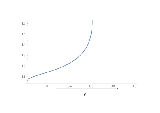
Figure 1: Graph of $\frac{\bar{F}_{1:N}(-\ln y)}{\bar{G}_{1:N}(-\ln y)}$

Remark 3.1

It can be checked that, in Theorem 3.1, if there exists stochastic ($st$) ordering between $X_{1:n}$ and $Y_{1:n}$ in place of $hr$ ordering, then without any condition as of the previous theorem, there will also exists $st$ ordering between $X_{1:N}$ and $Y_{1:N}$. The proof of it is very trivial. Same can be observed for Theorem 3.2-3.4 also.

The next few theorems can be proved in the same fashion as above and hence the details are omitted.

Theorem 3.2

Suppose $X_{1:n}\sim\bar{F}_{1:n}(x)$ and $Y_{1:n}\sim\bar{G}_{1:n}(x).$ Also let $N$ be a random variable having pmf $p(n).$ Now, for all $x\geq 0$, if $\frac{\bar{F}_{1:n}(x)}{\bar{G}_{1:n}(x)}$ is decreasing in $n\in\mathcal{N}^{+}$, then $X_{1:n}\geq_{hr}Y_{1:n}$ implies $X_{1:N}\geq_{hr}Y_{1:N}.$

Proof: The theorem can be proved using Lemma 3.2, Theorem 2.1 and following the proof of Theorem 3.1.

Theorem 3.3

Suppose $X_{n:n}\sim\bar{F}_{n:n}(x)$ and $Y_{n:n}\sim\bar{G}_{n:n}(x).$ Also let $N$ be a random variable having pmf $p(n).$ Now, for all $x\geq 0$, if $\overline{r}_{Y_{n:n}}(x)$, the reversed hazard rate function of $Y_{n:n}$ is increasing in $n\in\mathcal{N}^{+}$ and $\frac{F_{n:n}(x)}{G_{n:n}(x)}$ is decreasing in $n\in\mathcal{N}^{+}$, then $X_{n:n}\leq_{rh}Y_{n:n}$ implies $X_{N:N}\leq_{rh}Y_{N:N}.$

Proof: If $\overline{r}_{Y_{n:n}}(x)$ is increasing in $n$, then for any two positive integers $n_{1}\leq n_{2}$ and for all $x\geq 0$ it can be written that $\overline{r}_{Y_{n_{1}:n_{1}}}(x)\leq\overline{r}_{Y_{n_{2}:n_{2}}}(x)$, which can equivalently conclude that $\frac{G_{n_{1}:n_{1}}(x)}{G_{n_{2}:n_{2}}(x)}$ is decreasing in $x\geq 0$. Thus, the theorem can be proved using Lemma 3.3 and following the line of the proof of Theorem 3.1.

Theorem 3.4

Suppose $X_{n:n}\sim\bar{F}_{n:n}(x)$ and $Y_{n:n}\sim\bar{G}_{n:n}(x).$ Also let $N$ be a random variable having pmf $p(n).$ Now, for all $x\geq 0$, if $\overline{r}_{Y_{n:n}}(x)$, the reversed hazard rate function of $Y_{n:n}$ is increasing in $n\in\mathcal{N}^{+}$ and $\frac{F_{n:n}(x)}{G_{n:n}(x)}$ is decreasing in $n\in\mathcal{N}^{+}$, then $X_{n:n}\geq_{rh}Y_{n:n}$ implies $X_{N:N}\geq_{rh}Y_{N:N}.$

Proof: The theorem can be proved using Lemma 3.4 and following the proof of Theorem 3.3.

Remark 3.2

It is to be noted that Theorem 3.3 and 3.4 are proved with an additional condition that “for all $x\geq 0$, the reversed hazard rate function ($\overline{r}_{Y_{n:n}}(x)$) of $Y_{n:n}$ is increasing in $n$”, while no such condition is required to prove Theorems 3.1 and 3.2. This can be rationalized by Theorem 1.B.28 of Shaked and Shanthikumar ([20]) (see Theorem 2.1 above) which states that for all $x\geq 0$, the hazard rate function ($r_{Y_{1:n}}(x)$) of $Y_{1:n}$ is always increasing in $n$, which is not always true for reversed hazard rate function. In fact, Theorem 1.B.57 of Shaked and Shanthikumar ([20]) (see Theorem 2.2 above) uses more restrictive sufficient condition $X_{m}\leq_{rh}X_{j}$ for all $j=1,2,\ldots,m-1$ to prove similar result. Hence, one additional condition is used in Theorems 3.3 and 3.4 to avoid such restrictive sufficient conditions.

4 Conclusion

The paper aims to provide some new results on the comparison of extremes with random number of independent and non-identically distributed random variables. The variation diminishing property (Karlin [8]) is extended to all possible restrictions and the associated lemmas are proved which are used to derive the key results. The findings of this paper have not been studied in the literature to the best of our knowledge. Stochastic comparison of systems (series/parallel) where the components are non-identically distributed and are randomly chosen (randomized components) from two different batches can be an interesting problem for future research.

Disclosure statement
No potential conflict of interest was reported by the author(s).

References

- [1] Ahmad, I. and Kayid, M. (2007). Reversed preservation of stochastic orders for random minima and maxima with applications. Statistical Papers, 48, 283-293.
- [2] Balakrishnan, N. and Zhao, P. (2013). Ordering properties of order statistics from heterogeneous populations: A review with an emphasis on some recent developments. Probability in the Engineering and Informational Sciences, 27, 403-443.
- [3] Barmalzan, G., Najafabadi, A.T.P. and Balakrishnan, N. (2017). Ordering properties of the smallest and largest claim amounts in a general scale model. Scandinavian Actuarial Journal, 2017(2), 105–124.
- [4] Bartoszewicz, J. (2001). Stochastic comparisons of random minima and maxima from life distributions. Statistics & probability letters, 55(1), 107-112.
- [5] Chowdhury, S. and Kundu, A. (2017). Stochastic comparison of parallel systems with log-Lindley distributed components. Operations Research Letters, 45(3), 199-205.
- [6] Di Crescenzo, A. and Pellerey, F. (2011). Stochastic comparisons of series and parallel systems with randomized independent components. Operations Research Letters, 39(5), 380-384.
- [7] Hazra, N. K., Nanda, A. K. and Shaked, M. (2014). Some aging properties of parallel and series systems with a random number of components. Naval Research Logistics, 61(3), 238-243.
- [8] Karlin, S. (1968). Total Positivity. Stanford University Press, Stanford, CA.
- [9] Karlin, S. and Rinott, Y. (1980a). Classes of Orderings of Measures and Related Correlation Inequalities I. Multivariate Totally Positive Distributions. Journal of Multivariate Analysis, 10(4), 467-498.
- [10] Karlin, S. and Rinott, Y. (1980b). Classes of Orderings of Measures and Related Correlation Inequalities II. Multivariate Reverse Rule Distributions. Journal of Multivariate Analysis, 10(4), 499-516.
- [11] Koutras, M. V. and Milienos, F. S. (2017). A flexible family of transformation cure rate models. Statistics in medicine, 36(16), 2559-2575.
- [12] Koutsoyiannis, D. (2004). Statistics of extremes and estimation of extreme rainfall, 1, Theoretical investigation. Hydrological Sciences Journal, 49 (4), 575–590.
- [13] Kundu, A. and Chowdhury, S. (2016). Ordering properties of order statistics from heterogeneous exponentiated Weibull models. Statistics & Probability Letters, 114. 119-127.
- [14] Kundu, A. and Chowdhury, S. (2020). On stochastic comparisons of series systems with heterogeneous dependent and independent location-scale family distributed components. Operations Research Letters, 48(1), 40-47.
- [15] Li, X. and Zuo, M. J. (2004). Preservation of stochastic orders for random minima and maxima, with applications. Naval Research Logistics, 51(3), 332-344.
- [16] Nakagawa, T. and Zhao, X. (2012). Optimization problems of a parallel system with a random number of units. IEEE Transactions on Reliability, 61(2), 543-548.
- [17] Nanda, A. K. and Shaked, M. (2008). Partial ordering and aging properties of order statistics when sample size is random: a brief review. Communications in Statistics: Theory Methods, 37, 1710–1720.
- [18] Navarro, J., Pellerey, F. and Di Crescenzo, A. (2015). Orderings of coherent systems with randomized dependent components. European Journal of Operational Research, 240(1), 127-139.
- [19] Shaked, M. (1975). On the distribution of the minimum and of the maximum of a random number of i.i.d. random variables. In Statistical Distributions in Scientific Work. Vol. I. ed. G. P Patil, S. Kotz and J. K. Ord. Reidel, Dordrecht. pp. 363-380.
- [20] Shaked, M. and Shanthikumar, J.G. (2007). Stochastic Orders. Springer, New York.
- [21] Shaked, M. and Wong, T. (1997). Stochastic comparisons of random minima and maxima. Journal of Applied Probability, 34, 420 – 425.
- [22] Srivastava, R.C. (1973). Estimation of Probability Density Function based on Random Number of Observations with Applications. International Statistical Review, 41(1), 77-86.
- [23] Torrado, N. and Kochar, S.C. (2015). Stochastic order relations among parallel systems from Weibull distributions. Journal of Applied Probability, 52, 102-116.