At the end of the spectrum:
Chromatic bounds for the largest eigenvalue of the normalized Laplacian

Abstract

For a graph with largest normalized Laplacian eigenvalue $\lambda_{N}$ and (vertex) coloring number $\chi$, it is known that $\lambda_{N}\geq\chi/(\chi-1)$. Here we prove properties of graphs for which this bound is sharp, and we study the multiplicity of $\chi/(\chi-1)$. We then describe a family of graphs with largest eigenvalue $\chi/(\chi-1)$. We also study the spectrum of the $1$-sum of two graphs, with a focus on the maximal eigenvalue. Finally, we give upper bounds on $\lambda_{N}$ in terms of $\chi$.

Keywords: $1$-sum; Coloring number; Largest eigenvalue; Normalized Laplacian

1 Introduction

1.1 At the end of the color spectrum

As anyone who is familiar with more than one language knows, there are some things that you can express precisely in one language that you cannot in another, and vice versa. In many aspects, the evolution of different languages is somewhat arbitrary. There are, on the other hand, also universalities in the development of different languages, a notable one being basic color terms. In 1969, Berlin and Kay [4] identified different stages in the development of basic color terms for distinct languages. In Stage I, a distinction is developed between darker (black) and lighter shades (white). In Stage II, a word for the color red and adjacent shades is developed, and in Stage III, either a word for yellow or green shades emerges; in Stage IV, there are words for both yellow and green. This evolution continues: in Stage V, the word for blue is coined, in Stage VI, the word for brown appears, and in the final stages, four colors are added, not necessarily in a fixed order, until there are exactly eleven terms for the basic colors: black, white, red, green, yellow, blue, brown, purple, pink, orange and grey.

Berlin and Kay studied which of the eleven basic color terms were in the vocabulary of different languages from different families, and encountered only $22$ combinations of these eleven colors, out of $2048$ possible combinations. It thus appears that the evolution of basic color terms is a constant in the development of a language: following more or less the same pattern, the same eleven basic color terms appear in the vocabulary of any language, to describe a spectrum of colors.

A field in which both colors and spectra are studied, is graph theory: in spectral graph theory, spectra of different matrices associated with a graph are studied, and in chromatic graph theory[10, 3], different notions of colorings of a graph are studied. In this paper, we combine these branches of graph theory, by studying bounds relating the largest eigenvalue of the normalized Laplacian of a graph to its vertex coloring number.

1.2 At the end of the Laplacian spectrum

The context in which we shall work is the following. Let $G=(V,E)$ be a finite simple graph, i.e., an undirected, unweighted graph without multi-edges and without loops, with $N$ vertices $v_{1},\ldots,v_{N}$. Two distinct vertices $v$ and $w$ are called adjacent, denoted $v\sim w$ or $w\sim v$, if $\{v,w\}\in E$. The degree $\deg_{G}v$ or $\deg v$ of a vertex $v$ is the number of vertices that it is adjacent to. If the degree of every vertex of $G$ is equal to some fixed positive integer $d$, then we say that $G$ is regular or $d$-regular. We assume that no vertex has degree $0$.

A (vertex) $k$-coloring is a function $c:V\to\{1,\ldots,k\}$, and it is proper if $v\sim w$ implies that $c(v)\neq c(w)$. The (vertex) coloring number or chromatic number $\chi=\chi(G)$ is the minimum $k$ such that there exists a proper $k$-coloring of the vertices. If $\chi(G)\leq 2$, then we say that $G$ is bipartite. These and other elementary definitions in graph theory can be found, for instance, in [17].

When determining the coloring number $\chi$ of a given graph $G$, one can find an upper bound $\chi\leq k$ by giving a proper $k$-coloring of the vertices of $G$. Finding lower bounds directly, by showing that a graph cannot admit a proper $k$-coloring for some $k$, requires more work in general. Therefore, it is useful to find lower bounds in another way, for example, by considering the spectrum of a matrix associated with $G$.

Given a graph $G$, four notable matrices whose spectra are studied in spectral graph theory, are the adjacency matrix, the Kirchoff Laplacian, the signless Laplacian and the normalized Laplacian. The adjacency matrix of $G$ is the $N\times N$ matrix $A\coloneqq A(G)$ with entries

$$A_{ij}\coloneqq\begin{cases}1&\text{ if }v_{i}\sim v_{j}\\ 0&\text{ otherwise.}\end{cases}$$

The Kirchoff Laplacian is the matrix $K\coloneqq K(G)\coloneqq D-A$, and the signless Laplacian is the matrix $Q\coloneqq Q(G)\coloneqq D+A$, where $D\coloneqq\operatorname{diag}\bigl{(}\deg v_{1},\ldots,\deg v_{N}\bigr{)}$. The spectrum of the adjacency matrix, especially for regular graphs, and of the Kirchoff Laplacian have been studied, for instance, in [17, 15, 5]. Literature on the signless Laplacian can be found in [14].

In 1992, Chung [12] introduced the matrix

$$\mathcal{L}:=\mathcal{L}(G):=\operatorname{Id}-D^{-1/2}AD^{-1/2},$$

where $\operatorname{Id}$ denotes the $N\times N$ identity matrix. The matrix $\mathcal{L}$ is similar (in matrices terms) to the normalized Laplacian of $G$, which is defined as

$$L:=L(G):=\operatorname{Id}-D^{-1}A.$$

In fact, $L=D^{-1/2}\mathcal{L}D^{1/2}$. Therefore, given a graph $G$, the spectra of $L$ and $\mathcal{L}$ coincide. Here we shall focus on $L$. Its entries are

$$L_{ij}=\begin{cases}1&\text{ if }i=j\\ -\frac{1}{\deg v_{i}}&\text{ if }v_{i}\sim v_{j}\\ 0&\text{ otherwise.}\end{cases}$$

In particular, for $v_{i}\sim v_{j}$, $-L_{ij}$ is the probability of going from $v_{i}$ to $v_{j}$ with a classical random walk on $V$.

The spectra of the four matrices $A$, $K$, $Q$ or $L$ can be used to find different information about $G$. For example, from the spectrum of the adjacency matrix, one can derive the number of edges of $G$, which is not possible from the normalized Laplacian spectrum, whereas the multiplicity of the eigenvalue $0$ in the normalized Laplacian spectrum equals the number of connected components, which is information that the adjacency spectrum cannot give you.

Sometimes one language provides you with the words to say something that you cannot say in another. Similarly, there are graphs which have the same spectrum with respect to one matrix — we say that they are cospectral with respect to that matrix — but they have different spectra with respect to another. For example, all complete bipartite graphs with the same number of vertices have the same normalized Laplacian spectrum, but not the same adjacency spectrum.

In the same way that the evolution of basic color terms is a constant factor in the development of a language, we have that $d$-regular graphs are in some way a constant factor in spectral analysis of the aforementioned graphs: if a graph $G$ is $d$-regular, then the spectrum of one among $A$, $K$, $Q$ and $L$, determines the spectrum of the other three. In fact, in this case, we have that $D=d\cdot\operatorname{Id}$, implying that $K=d\cdot\operatorname{Id}-A$ and $\mathcal{L}=L=\frac{1}{d}\cdot K$. Hence, for $d$-regular graphs,

$$\lambda\text{ is an eigenvalue for }K \iff d-\lambda\text{ is an eigenvalue for }A$$

$$\iff\frac{\lambda}{d}\text{ is an eigenvalue for }\mathcal{L}=L.$$

This also implies that two $d$-regular graphs $G_{1}$ and $G_{2}$ are cospectral with respect to one matrix if and only if they are cospectral with respect to another.

Problems in spectral graph theory include finding cospectral graphs, as well as finding graphs that are determined by their spectrum, with respect to some of the four matrices that we defined. Other questions concern themselves with relating the spectrum of one of the matrices to other graph properties. An example of a well-known result is the Hoffman bound [19], which gives a lower bound on the vertex coloring number using the smallest and largest adjacency eigenvalues. This bound has been generalized to include more eigenvalues [32].

We are, in this paper, interested in the normalized Laplacian spectrum. We let

$$\lambda_{N}\geq\lambda_{N-1}\geq\cdots\geq\lambda_{1}=0$$

denote the eigenvalues of $L$, and we also introduce the notation $\lambda_{\max}:=\lambda_{N}$. We have that $0\leq\lambda\leq 2$ for every eigenvalue $\lambda$ of $L$. The multiplicity of the eigenvalue $0$ equals the number of connected components, and the multiplicity of the eigenvalue $2$ equals the number of bipartite components. More background on the normalized Laplacian spectrum can be found in [12, 8, 9, 7].

Since the normalized Laplacian spectrum of a graph equals the union of the spectra of its connected components, we assume for the rest of the paper that $G$ is connected. We also assume that $N\geq 2$. The normalized Laplacian eigenvalues that are studied the most, are the second smallest and the largest. It is known, for example, that the largest eigenvalue equals $2$ if and only if $G$ is bipartite, while it is equal to $N/(N-1)$ if and only if $G$ is the complete graph. For all other graphs, we have that $\lambda_{N}\geq(N+1)/(N-1)$ [26, 20]. Some other problems involving the normalized Laplacian regard multiplicities, for example: Which graphs have two normalized Laplacian eigenvalues, and which graphs have three normalized Laplacian eigenvalues [31]? The answer to the first question is: only complete graphs, while the answer to the second question is not known.

Other questions include: Which graphs are determined by their spectrum? Which graphs have an eigenvalue with multiplicity $N-2$ [31], and which graphs have an eigenvalue with multiplicity $N-3$ [25, 29]? How do the eigenvalues change when deleting an edge of $G$ [6]? How does the spectrum change under other graph operations [11]?

As we saw before, we have, given $N$, that bipartite graphs have the largest possible largest eigenvalue, whereas the complete graph has the smallest possible largest eigenvalue. In some other sense, bipartite graphs and complete graphs are also on opposite ends of a spectrum: the former has the smallest possible coloring number, and the latter has the largest possible coloring number given $N$. In both cases, we have that $\lambda_{N}=\chi/(\chi-1)$. Sun and Das [27] proved that, in general, we have the inequality

$$\lambda_{N}\geq\frac{\chi}{\chi-1},$$

which coincides with the Hoffman bound for regular graphs. Moreover, they observed that the inequality is sharp for both bipartite and complete graphs.

In this paper, we study more graphs for which this inequality is sharp. These graphs are special, as they relate to some of the aforementioned problems, regarding the smallest possible value of $\lambda_{N}$ in terms of $N$, and graphs with a largest eigenvalue of multiplicity $N-2$ and $N-3$.

2 Background

2.1 Basic definitions, notations and properties

In this section we shall introduce some more definitions, notations and properties that we shall refer to throughout the paper. As in the Introduction, we fix a simple graph $G=(V,E)$ on $N$ vertices, we assume that $G$ is connected, and we let $v_{1},\ldots,v_{N}$ denote its vertices.

We start by listing several properties of the normalized Laplacian of $G$ and its spectrum.

Remark 2.1.

Let $C(V)$ denote the vector space of functions $f:V\rightarrow\mathbb{R}$ and, given $f,g\in C(V)$, let

$$\langle f,g\rangle:=\sum_{v\in V}\deg v\cdot f(v)\cdot g(v).$$

We can see the normalized Laplacian $L$ as an operator $C(V)\rightarrow C(V)$ such that

$$Lf(v)=f(v)-\frac{1}{\deg v}\sum_{w\sim v}f(w).$$ (1)

Also, it is easy to check that $L$ is self-adjoint with respect to the inner product $\langle\cdot,\cdot\rangle$, i.e.,

$$\langle Lf,g\rangle=\langle f,Lg\rangle\quad\forall f,g\in C(V).$$

Remark 2.2.

By (1), $(\lambda,f)$ is an eigenpair for $L$ if and only if, for all $v\in V$,

$$\lambda f(v)=f(v)-\frac{1}{\deg v}\sum_{w\sim v}f(w),$$

which can be equivalently rewritten as

$$(1-\lambda)f(v)=\frac{1}{\deg v}\sum_{w\sim v}f(w).$$ (2)

With the Courant-Fischer-Weyl min-max Principle below, we can characterize the eigenvalues of $L$.

Theorem 2.3 (Courant-Fischer-Weyl min-max Principle).

Let $H$ be an $N$-dimensional vector space with a positive definite scalar product $(.,.)$, and let $A:H\rightarrow H$ be a self-adjoint linear operator. Let $\mathcal{H}_{k}$ be the family of all $k$-dimensional subspaces of $H$. Then the eigenvalues $\lambda_{1}\leq\ldots\leq\lambda_{N}$ of $A$ can be obtained by

$$\lambda_{k}=\min_{H_{k}\in\mathcal{H}_{k}}\max_{g(\neq 0)\in H_{k}}\frac{(Ag,g)}{(g,g)}=\max_{{H}_{N-k+1}\in\mathcal{H}_{N-k+1}}\min_{g(\neq 0)\in{H}_{N-k+1}}\frac{(Ag,g)}{(g,g)}.$$ (3)

The vectors $g_{k}$ realizing such a min-max or max-min then are corresponding eigenvectors, and the min-max spaces $H_{k}$ are spanned by the eigenvectors for the eigenvalues $\lambda_{1},\dots,\lambda_{k}$, and analogously, the max-min spaces $H_{N-k+1}$ are spanned by the eigenvectors for the eigenvalues $\lambda_{k},\dots,\lambda_{N}$.

Thus, we also have

$$\lambda_{k}=\min_{g(\neq 0)\in H,(g,g_{j})=0\ \mathrm{for}\ j=1,\dots,k-1}\frac{(Ag,g)}{(g,g)}=\max_{g(\neq 0)\in H,(g,g_{\ell})=0\ \mathrm{for}\ \ell=k+1,\dots,N}\frac{(Ag,g)}{(g,g)}.$$ (4)

In particular,

$$\lambda_{1}=\min_{g(\neq 0)\in H}\frac{(Ag,g)}{(g,g)},\qquad\lambda_{N}=\max_{g(\neq 0)\in H}\frac{(Ag,g)}{(g,g)}.$$ (5)

Definition 2.4.

$(Ag,g)/(g,g)$ is called the Rayleigh quotient of $g$.

According to Theorem 2.3, the eigenvalues of $L$ are given by minimax values of

$$\textrm{RQ}(f):=\frac{\langle Lf,f\rangle}{\langle f,f\rangle}=\frac{\sum_{v\sim w}\biggl{(}f(v)-f(w)\biggr{)}^{2}}{\sum_{v\in V}\deg v\cdot f(v)^{2}},\quad\text{for }f\in C(V).$$

In particular, let $k\in\{1,\ldots,N\}$ and let $g_{i}$ be an eigenfunction for $\lambda_{i}$, for each $i\in\{1,\ldots,N\}\setminus\{k\}$. Then,

$$\lambda_{k}=\min_{\begin{subarray}{c}f\in C(V)\setminus\{\mathbf{0}\}:\\ \langle f,g_{1}\rangle=\ldots=\langle f,g_{k-1}\rangle=0\end{subarray}}\textrm{RQ}(f)=\max_{\begin{subarray}{c}f\in C(V)\setminus\{\mathbf{0}\}:\\ \langle f,g_{k+1}\rangle=\ldots=\langle f,g_{N}\rangle=0\end{subarray}}\textrm{RQ}(f),$$

and the functions realizing such a min-max are the corresponding eigenfunctions for $\lambda_{k}$.

Remark 2.5.

The largest eigenvalue of the corresponding normalized Laplacian can be characterized by

$$\lambda_{N}=\max_{f:V\rightarrow\mathbb{R}}\frac{\sum_{v\sim w}\biggl{(}f(v)-f(w)\biggr{)}^{2}}{\sum_{v\in V}\deg v\cdot f(v)^{2}}.$$

Furthermore, any function $f\in C(V)\setminus\{\boldsymbol{0}\}$ attaining this maximum is an eigenfunction of $L$ with eigenvalue $\lambda_{N}$.

We shall now give the definitions of independent sets, twin vertices and duplicate vertices.

Definition 2.6.

Let $U\subseteq V$. We say that $U$ is an independent set if, for all pairs of vertices $u_{1},u_{2}\in U$, we have that $u_{1}\not\sim u_{2}$.

Definition 2.7.

Given $u\in V$, we let $N(u)$ denote the set of all neighbors of $u$, i.e., the set of all vertices that are adjacent to $u$. If two distinct vertices $v,w\in V$ have the property that

$$N(v)\setminus\{w\}=N(w)\setminus\{v\},$$

then $v$ and $w$ are twin vertices if $v\sim w$, while $v$ and $w$ are duplicate vertices if $v\not\sim w$.

We refer to [7] for an extensive study of twin vertices, duplicate vertices and twin subgraphs.

Definition 2.8.

Let $U_{1},U_{2}\subset V$ be subsets of the vertex set of $G$. We let

$$e\bigl{(}U_{1},U_{2}\bigr{)}\coloneqq\bigl{|}\bigl{\{}\{u,v\}\in E\colon u\in U_{1},v\in U_{2}\bigr{\}}\bigr{|}.$$

Moreover, if $U_{1}=\{v\}$ for some $v\in V$, we let

$$e\bigl{(}v,U_{2}\bigr{)}\coloneqq e\bigl{(}\{v\},U_{2}\bigr{)}.$$

Definition 2.9.

Let $v,w\in V$ be distinct vertices. We let

$$f_{v,w}(u)\coloneqq\begin{cases}1,&\text{ if }u=v,\\ -1,&\text{ if }u=w,\\ 0,&\text{ otherwise.}\end{cases}$$

Definition 2.10.

Fix a proper $k$-coloring of $G$ with coloring classes $V_{1},\ldots,V_{k}$. Given two distinct indices $i,j\in\{1,\ldots,k\}$, we define $f_{ij}\colon V\to\mathbb{R}$ by

$$f_{ij}(v)\coloneqq\begin{cases}1,&\text{ if }v\in V_{i},\\ -1,&\text{ if }v\in V_{j},\\ 0,&\text{ otherwise.}\end{cases}$$

Note that, if $G$ bipartite and $V_{1}$ and $V_{2}$ denote its bipartition classes, then the function $f_{12}$ from Definition 2.10 has the property that

$$\textrm{RQ}(f_{12})=2=\lambda_{N}=\frac{\chi}{\chi-1}.$$

If $G$ is a complete graph, then any function $f_{ij}$ from Definition 2.10 is of the form $f_{v,w}$ as in Definition 2.9 for some $v,w\in V$, and it has the property that

$$\textrm{RQ}(f_{ij})=\frac{N}{N-1}=\lambda_{N}=\frac{\chi}{\chi-1}.$$

2.2 Given families of graphs with corresponding coloring number and spectrum

We shall now list some special graphs, together with their coloring number and their spectrum with respect to the normalized Laplacian. A more elaborate list of graphs and their spectra, also including the spectra with respect to other matrices than the normalized Laplacian, can be found in [9]. We use the notation

$$\bigl{\{}\mu_{1}^{(m_{1})},\ldots,\mu_{p}^{(m_{p})}\bigr{\}}$$

to denote a multiset which contains the element $\mu_{i}$ with multiplicity $m_{i}$. Throughout the paper, we shall also use the notation $m_{G}(\lambda)$ for the multiplicity of $\lambda$ as an eigenvalue of the normalized Laplacian of $G$.

1. The complete graph $K_{N}$ on $N$ vertices has coloring number $\chi=N$ and spectrum

   $$\biggl{\{}\frac{N}{N-1}^{(N-1)},0^{(1)}\biggr{\}}.$$

2. The complete bipartite graph $K_{N_{1},N_{2}}$ on $N=N_{1}+N_{2}$ vertices has coloring number $\chi=2$ and spectrum

   $$\biggl{\{}2^{(1)},1^{(N-2)},0^{(1)}\biggr{\}}.$$

   A special example is the star graph $S_{N}=K_{N-1,1}$.

3. The complete multipartite graph with partition classes of the same size $K_{\underbrace{N_{1},\ldots,N_{1}}_{k}}$ on $N=k\cdot N_{1}$ vertices, which can be equivalently described as the Turán graph $T(N,k)$ [30, 23, 16], has coloring number $\chi=k$ and spectrum

   $$\biggl{\{}\frac{k}{k-1}^{(k-1)},1^{(N-k)},0^{(1)}\biggr{\}}.$$

4. The $m$-petal graph [21] on $N=2m+1$ vertices is the graph with vertex set

   $$V=\{y,v_{1},\ldots,v_{m},w_{1},\ldots,w_{m}\}$$

   and edge set

   $$E=\bigcup_{i=1}^{m}\biggl{\{}\{x,v_{i}\},\{x,w_{i}\},\{v_{i},w_{i}\}\biggr{\}}.$$

   An example can be found in Figure 4(a) below. Its coloring number $\chi$ equals $3$, and its spectrum is

   $$\biggl{\{}\frac{3}{2}^{(m+1)},\frac{1}{2}^{(m-1)},0^{(1)}\biggr{\}}.$$

3 Graphs with largest eigenvalue $\chi/(\chi-1)$

Also in this section we fix a connected simple graph $G=(V,E)$ on $N\geq 2$ vertices.

The following theorem gives a lower bound for the maximum eigenvalue of the normalized Laplacian of a graph in terms of its coloring number, and it was proven by Coutinho, Grandsire and Passos (2019) [13] (Lemma 3.3) and by Sun and Das (2020) [27] (Theorem 3.1). A generalization for hypergraphs was proven by Abiad, Mulas and Zhang (2021) [1].

Theorem 3.1.

We have that

$$\lambda_{N}\geq\frac{\chi}{\chi-1},$$

and this inequality is sharp.

In [27], Sun and Das state the following open question:

Question 1.

Which connected finite graphs satisfy $\lambda_{N}=\chi/(\chi-1)$?

They also give a couple of graphs for which this equality holds, including complete multipartite graphs with partition classes of equal size, and $m$-petal graphs (cf. Section 2.2 and [21]). In the following theorem we give a necessary property for graphs with largest eigenvalue $\chi/(\chi-1)$. This result was first proven in [13], and we offer a shorter alternative proof.

Theorem 3.2 (Coutinho, Grandsire & Passos (2019), Corollary 4.7).

Assume that $\lambda_{N}=\chi/\bigl{(}\chi-1\bigr{)}$, and fix a proper $\chi$-coloring with coloring classes $V_{1},V_{2},\ldots,V_{\chi}$. Then, for all $i=1,\ldots,\chi$ and all $v\in V_{i}$, we have that

$$e(v,V_{i})=\begin{cases}\frac{\deg v}{\chi-1}&\text{ if }v\notin V_{i},\\ 0&\text{ if }v\in V_{i}.\end{cases}$$

Proof.

Without loss of generality, we may assume that

$$e\bigl{(}V_{1},V_{2}\bigr{)} =\max_{U_{1},U_{2}\text{ coloring classes with respect to\ }c}e\bigl{(}U_{1},U_{2}\bigr{)}.$$ (6)

Let $W\coloneqq V\setminus\bigl{(}V_{1}\cup V_{2}\bigr{)}$, and consider the function $f_{12}$ from Definition 2.10. We have that

$$\textrm{RQ}\bigl{(}f_{12}\bigr{)} =\frac{\sum_{v\sim w}\bigl{(}f_{12}(v)-f_{12}(w)\bigr{)}^{2}}{\sum_{v\in V}\deg v\cdot f_{12}(v)^{2}}$$

$$=1-2\frac{\sum_{v\sim w}f_{12}(v)\cdot f_{12}(w)}{\sum_{v\in V}\deg v\cdot f_{12}(v)^{2}}$$

$$=1+\frac{2\cdot e(V_{1},V_{2})}{2e\bigl{(}V_{1},V_{2}\bigr{)}+e\bigl{(}V_{2},W\bigr{)}+e\bigl{(}V_{1},W\bigr{)}}.$$

Moreover, it follows from (6) that

$$e\bigl{(}V_{1},W\bigr{)}+e\bigl{(}V_{2},W\bigr{)} =\sum_{i=3}^{\chi}e\bigl{(}V_{1},V_{i}\bigr{)}+\sum_{i=3}^{\chi}e(V_{2},V_{i})$$

$$\overset{\eqref{eq:e(V1,V2)}}{\leq}2\sum_{i=3}^{\chi}e\bigl{(}V_{1},V_{2}\bigr{)}$$

$$=2\bigl{(}\chi-2\bigr{)}e(V_{1},V_{2}).$$

We use this inequality to obtain

$$\begin{split}\textrm{RQ}(f_{12})&=1+\frac{2e\bigl{(}V_{1},V_{2}\bigr{)}}{2e\bigl{(}V_{1},V_{2}\bigr{)}+e\bigl{(}V_{2},W\bigr{)}+e\bigl{(}V_{1},W\bigr{)}}\\ &\geq 1+\frac{2e(V_{1},V_{2})}{2e(V_{1},V_{2})+2(\chi-2)e(V_{1},V_{2})}\\ &=\frac{\chi}{\chi-1}.\end{split}$$ (7)

Together with the assumption that $\lambda_{N}=\chi/(\chi-1)$, this implies that

$$\textrm{RQ}(f_{12})=\frac{\chi}{\chi-1}.$$

Hence, the inequality (7) must be an equality, implying that

$$e(V_{1},V_{2})=e(V_{1},V_{i}),\quad\text{for $i=3,\ldots,\chi$.}$$

We can thus, for $i=3,\ldots,\chi$, calculate $\textrm{RQ}(f_{1i})$ analogously to $\textrm{RQ}(f_{12})$, to see that

$$\textrm{RQ}(f_{1i})=\frac{\chi}{\chi-1}=\lambda_{N},\quad\text{for $i=2,\ldots,\chi$.}$$

As a consequence, we have that

$$e(V_{1},V_{2})=e(V_{1},V_{i})=e(V_{i},V_{j}),\quad\text{for $1\leq j\leq\chi$ such that $j\neq i$.}$$

We can use this to see that

$$\textrm{RQ}(f_{ij})=\frac{\chi}{\chi-1}=\lambda_{N},\quad\text{for $1\leq i<j\leq\chi$.}$$

Now let $v\in V(G)$, and let $i$ be such that $v\in V_{i}$. Then, by definition of proper $\chi$-coloring, we have that $e(v,V_{i})=0$. Now consider $j\neq i$ such that $1\leq j\leq\chi$. By the min-max Principle (3), we have that $(\chi/(\chi-1),f_{ij})$ is an eigenpair of $L$. Equation (2) gives us that

$$\frac{1}{\chi-1}=\frac{1}{\deg v}\cdot e(v,V_{j}).$$

By rewriting this, we conclude that

$$e(v,V_{i})=\begin{cases}\frac{\deg v}{\chi-1}&\text{ if }v\notin V_{i},\\ 0&\text{ if }v\in V_{i}.\end{cases}\qed$$

Example 3.3.

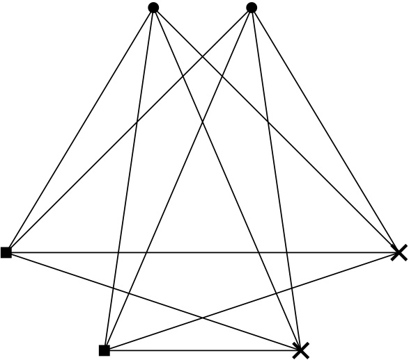
(a) The complete tripartite graph $K_{2,2,2}$

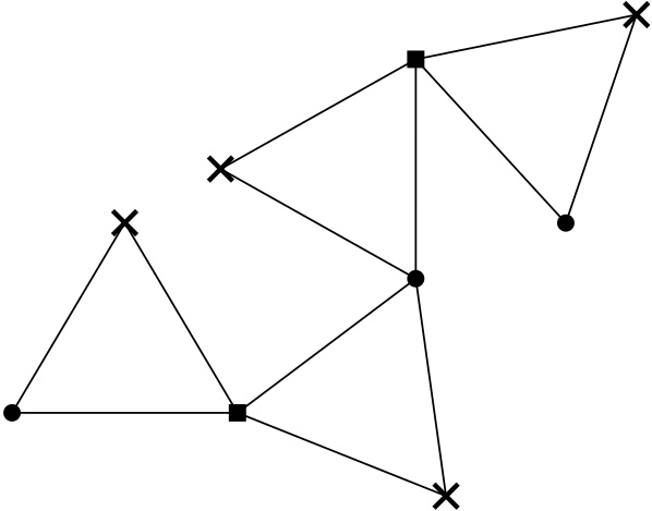
(b) A graph consisting of four triangles that are glued together

Figure 1: Two graphs with largest eigenvalue $\chi/(\chi-1)$

In Figure 1, two graphs with coloring number $\chi=3$ and largest eigenvalue $\chi/(\chi-1)=3/2$ are depicted. The graph in Figure 1(a) is the complete tripartite graph $K_{2,2,2}$ with partition classes of the same size, for which Sun and Das [27] proved that the largest eigenvalue equals $3/2$. In Section 5, we shall see that the graph in Figure 1(b) has largest eigenvalue $3/2$, because it consists of four triangles that are glued together.

In the figure, also a $\chi$-coloring of the vertices is indicated by the shape of the vertices. One can check that the result of Theorem 3.2 holds up for both graphs. Note that $K_{2,2,2}$ admits a unique $3$-coloring, but the graph in Figure 1(b) admits multiple $3$-colorings, and for all of these, we have by Theorem 3.2 that the neighbors of every vertex are spread evenly over the coloring classes.

Note that we can use our estimate of $\textrm{RQ}(f_{12})$ from the proof of Theorem 3.2 in combination with the min-max Principle (3), to see that, for any graph with coloring number $\chi$, we have that

$$\lambda_{N}\geq\textrm{RQ}(f_{12})\geq\frac{\chi}{\chi-1},$$

which gives an alternative proof of Theorem 3.1.

The following is a direct corollary of the proof of Theorem 3.2.

Corollary 3.4.

We have that $\lambda_{N}=\chi/(\chi-1)$ if and only if the following two statements both hold:

1. The function $f_{12}$ from Definition 2.10 maximizes the Rayleigh quotient;

2. For all $i=1,\ldots,\chi$ and all $v\in V$, we have that

   $$e(v,V_{i})=\begin{cases}\frac{\deg v}{\chi-1}&\text{ if }v\notin V_{i},\\ 0&\text{ if }v\in V_{i}.\end{cases}$$

We shall now prove some statements about graphs that have largest eigenvalue $\chi/(\chi-1)$. We start with a direct corollary of (the proof of) Theorem 3.2.

Corollary 3.5.

Assume that $\lambda_{N}=\chi/\bigl{(}\chi-1\bigr{)}$, and fix a proper $\chi$-coloring with coloring classes $V_{1},V_{2},\ldots,V_{\chi}$. For all $1\leq i<j\leq n$, we have that $f_{ij}$ from Definition 2.10 is an eigenfunction of $L$ for $\lambda_{N}$.

The above result has the following corollary, which also appears in the proof of Theorem 4.6 in [13].

Corollary 3.6.

If $\lambda_{N}=\chi/\bigl{(}\chi-1\bigr{)}$, then the multiplicity of the eigenvalue $\chi/\bigl{(}\chi-1\bigr{)}$ is at least $\chi-1$.

Proof.

This follows because, by Corollary 3.5, the functions $f_{1i}$, with $2\leq i\leq\chi$, are linearly independent eigenfunctions of $L$. Therefore, we see that the dimension of the eigenspace of the eigenvalue $\chi/\bigl{(}\chi-1\bigr{)}$ equals at least $\chi-1$. ∎

Conversely, for a graph that has largest eigenvalue $\chi/(\chi-1)$ with multiplicity equal to $\chi-1$, the following proposition holds.

Proposition 3.7.

If $\lambda_{N}=\chi/(\chi-1)$ and $\chi/(\chi-1)$ has multiplicity equal to $\chi-1$, then $G$ admits only one proper $\chi$-coloring, up to a permutation of the coloring classes.

Proof.

Let $c_{1}$ and $c_{2}$ be two proper $\chi$-colorings with coloring classes $V_{1}^{1},\ldots,V_{\chi}^{1}$ and $V_{1}^{2},\ldots,V_{\chi}^{2}$, respectively. Let $f_{ij}^{1}$ and $f_{ij}^{2}$ denote the functions from Definition 2.10 with respect to $c_{1}$ and $c_{2}$, respectively. Then, the eigenspace of $\lambda_{N}$ equals $E_{\chi/(\chi-1)}=\langle f^{1}_{1i}\colon 2\leq i\leq\chi\rangle$. This implies that

$$f_{1j}^{2}\in\langle f^{1}_{1i}\colon 2\leq i\leq\chi\rangle$$

for all $2\leq j\leq\chi$, which is only possible if, for any $2\leq j\leq\chi$, we have that $f^{2}_{1j}=f^{1}_{i,k(j)}$ for some fixed $i$ and $k(j)\neq i$ which depends on $j$. We conclude that the set of coloring classes of $c_{2}$ is the same as the set of coloring classes of $c_{1}$. ∎

In Section 4 we shall see that the opposite implication of Proposition 3.7 is not true.

As shown by Sun and Das in [27], one example of a graph with largest eigenvalue $\chi/(\chi-1)$ for which the multiplicity of $\chi/(\chi-1)$ equals $\chi-1$ is given by complete multipartite graphs with partition classes of the same size:

Theorem 3.8.

[Theorem 3.6 in [27]] Let $G$ be a complete multipartite graph with chromatic number $\chi\geq 3$. Then, the size of each partition is the same if and only if $\lambda_{N}=\chi/(\chi-1)$.

In Section 4 we shall also see more examples of graphs with largest eigenvalue $\chi/(\chi-1)$ for which the multiplicity of $\chi/(\chi-1)$ equals $\chi-1$.

We shall now prove a proposition about graphs with largest eigenvalue $\chi/(\chi-1)$ regarding their twin and duplicate vertices (cf. Definition 2.7).

Proposition 3.9.

Assume that $\lambda_{N}=\chi/\bigl{(}\chi-1\bigr{)}$.

1. If $v_{1}\sim v_{2}$ are twin vertices, then

   $$\deg v_{1}=\deg v_{2}=\chi-1.$$

   Moreover, the function $f_{v_{1},v_{2}}$ from Definition 2.9 is an eigenfunction with eigenvalue $\chi/(\chi-1)$.

2. If $w_{1}\not\sim w_{2}$ are duplicate vertices, then for any proper $\chi$-coloring, $w_{1}$ and $w_{2}$ must be in the same coloring class.

Proof.

1. Let $V_{1},\ldots,V_{\chi}$ be the coloring classes of $G$ with respect to a fixed proper $\chi$-coloring. Without loss of generality, we may assume that $v_{1}\in V_{1}$ and $v_{2}\in V_{2}$. Since $v_{1}$ and $v_{2}$ are twin vertices, we must have

   $$e(v_{1},V_{2})=e(v_{2},V_{1})=1,$$

   from which it follows by Theorem 3.2 that

   $$\deg v_{1}=\deg v_{2}=\chi-1.$$

   Moreover, since one can easily check that $\textrm{RQ}(f_{v_{1},w_{1}})=\chi/(\chi-1)$, we have that the function $f_{v_{1},v_{2}}$ is an eigenfunction with eigenvalue $\chi/(\chi-1)$.

2. Let $c$ be a proper $\chi$-coloring and assume, by contradiction, that $w_{1}$ and $w_{2}$ are not in the same coloring class. Then, the proper $\chi$-coloring $c^{\prime}$ defined by

   $$c^{\prime}(v)\coloneqq\begin{cases}c(w_{1})&\text{ if }v=w_{2},\\ c(v)&\text{ otherwise,}\end{cases}$$

   does not satisfy the statement of Theorem 3.2, which is a contradiction.∎

In [7], Butler proved the following result.

Proposition 3.10 (Corollary $1$ in [7]).

1. Let $D_{i}$ consist of a collection of duplicate vertices. Then there are $|D_{i}|-1$ eigenvalues of $1$ which come from eigenvectors restricted to $D_{i}$.

2. Let $T_{i}$ consist of a collection of twin vertices which have common degree $d$. Then there are $|T_{i}|-1$ eigenvalues of $(d+1)/d$ which come from eigenvectors restricted to $T_{i}$.

Remark 3.11.

Consider the setting of Proposition 3.10 and write

$$D_{i}=\left\{v_{1}^{(i)},\ldots,v_{|D_{i}|}^{(i)}\right\},\quad T_{i}=\left\{w_{1}^{(i)},\ldots,w_{|T_{i}|}^{(i)}\right\}.$$

Then, the eigenfunctions corresponding to the eigenvalue $1$ are of the form $f_{v_{1}^{(i)},v_{j}^{(i)}}$ as in Definition 2.9, for $2\leq j\leq|D_{i}|$. Analogously, as in part $1$ of Proposition 3.9, the eigenfunctions corresponding to the eigenvalue $d/(d+1)$ are of the form $f_{w_{1}^{(i)},w_{j}^{(i)}}$, for $2\leq j\leq|T_{i}|$.

We can use Proposition 3.10 to find upper and lower bounds for the multiplicity of $\chi/(\chi-1)$.

Proposition 3.12.

Assume that $\lambda_{N}=\chi/\bigl{(}\chi-1\bigr{)}$, and fix a proper $\chi$-coloring with coloring classes $V_{1},V_{2},\ldots,V_{\chi}$. Given $j\geq 0$ and $k\geq 0$, let

$$D_{1},\ldots,D_{j}\subseteq V(G)\quad\text{ and }\quad T_{1},\ldots,T_{k}\subseteq V(G)$$

be mutually disjoint sets such that $D_{1},\ldots,D_{j}$ form a collection of duplicate vertices, while $T_{1},\ldots,T_{k}$ form a collection of twin vertices. Moreover, fix the smallest $y$ such that

$$\bigcup_{i=1}^{j}T_{i}\subseteq V_{1}\cup\cdots\cup V_{y},$$

where we change the order of the coloring classes $V_{i}$ if necessary, and we let $y=0$ if $j=0$. Then,

$$\sum_{i=1}^{j}|T_{i}|-j+\chi-y\leq m_{G}\left(\frac{\chi}{\chi-1}\right)\leq N-\sum_{i=1}^{k}|D_{i}|+k-1.$$ (8)

Furthermore, the upper bound is tight if and only if $\bigcup_{i=1}^{k}D_{i}=V(G)$ and $G$ is a complete multipartite graph with partition classes of equal size.

Proof.

We first prove the lower bound. By part $2$ of Proposition 3.10, we have $\sum_{i=1}^{j}|T_{i}|-j$ linearly independent eigenfunctions with eigenvalue $\chi/(\chi-1)$, which come from eigenvectors restricted to $T_{i}$. Furthermore, the functions $f_{1m}$ from Definition 2.10, for $y+1\leq m\leq\chi$, which are eigenfunctions with eigenvalue $\chi/(\chi-1)$, are linearly independent from each other, and from the eigenfunctions that are restricted to $T_{i}$. This proves the lower bound in (8).

We shall now prove the upper bound. By part $1$ of Proposition 3.10, the eigenvalue $1$ has multiplicity at least $\sum_{i=1}^{k}|D_{i}|-k$. Furthermore, we know that the eigenvalue $0$ has multiplicity $1$. This proves the upper bound in (8).

It is left to prove that the upper bound is tight if and only if $\bigcup_{i=1}^{k}D_{i}=V(G)$ and $G$ is a complete multipartite graph with partition classes of equal size. It can be easily seen that, for complete multipartite graphs with partition classes of the same size, the bound is tight if $\bigcup_{i=1}^{k}D_{i}=V(G)$.

Conversely, if the upper bound is tight, then $G$ has exactly three eigenvalues: $0$, $1$ and $\chi/(\chi-1)$. Let $m_{1}$ and $m_{\chi/(\chi-1)}$ denote the multiplicities of $1$ and $\chi/(\chi-1)$, respectively. Then, $m_{1}$ and $m_{\chi/(\chi-1)}$ need to satisfy the two equations below.

$$N =m_{1}+m_{\chi/(\chi-1)}\cdot\frac{\chi}{\chi-1};$$

$$N-1 =m_{1}+m_{\chi/(\chi-1)}.$$

From this, it follows that

$$m_{1}=N-\chi\text{ and }m_{\chi/(\chi-1)}=\chi-1.$$

Since $m_{\chi/(\chi-1)}=\chi-1$, it follows by Proposition 3.7 that there is exactly one proper $\chi$-coloring of $G$, up to permutation of the coloring classes. Let $V_{1},\ldots,V_{\chi}$ denote the coloring classes with respect to such a proper $\chi$-coloring.

Since we are assuming that the upper bound is tight, we must have that all eigenfunctions with eigenvalue $1$ come from pairs of duplicate vertices. This is only possible if, for every coloring class $V_{i}$, the vertices of $V_{i}$, which form an independent set, are pairwise duplicate. Now fix a coloring class $V_{i}$, and fix $v\notin V_{i}$. Then, $e(v,V_{i})\in\{0,|V_{i}|\}$, since the vertices in $V_{i}$ are pairwise duplicate. If $e(v,V_{i})=0$, then by Theorem 3.2 we have that $\deg v=0$, which is a contradiction since we assume that $G$ is connected. Therefore, $v$ must be adjacent to all of the vertices $V_{i}$, implying that $G$ is complete multipartite.

For $G$ to have largest eigenvalue $\chi/(\chi-1)$, we must have that the coloring classes all have the same size by Theorem 3.8, which concludes our proof. ∎

Examples of graphs for which the lower bound from Proposition 3.12 is tight include complete multipartite graphs with partition classes of the same size, complete graphs, bipartite graphs, and petal graphs (cf. Section 2.2 and [21]).

4 Graphs with equal edge spread

In view of Theorem 3.2, it is natural to ask the following question.

Question 2.

Is it true that $\lambda_{N}=\chi/(\chi-1)$ if and only if, for every proper $\chi$-coloring, its coloring classes $V_{1},\ldots,V_{\chi}$ are such that

$$e\bigl{(}v,V_{i}\bigr{)}=\begin{cases}\frac{\deg v}{\chi-1}&\text{ if }v\notin V_{i},\\ 0&\text{ if }v\in V_{i}?\end{cases}$$

By Theorem 3.2, the implication $(\Rightarrow)$ from Question 2 is true. This section is dedicated to showing that the other implication does not hold, hence the answer to the question is no.

As before, we fix a connected simple graph $G=(V,E)$ on $N\geq 2$ vertices throughout the section.

Proposition 4.1.

Fix a proper $\chi$-coloring and let $V_{1},\ldots,V_{\chi}$ denote the corresponding coloring classes. Assume that, for all $V_{i}$ and for all $v\in V\setminus V_{i}$ we have that

$$e(v,V_{i})=\begin{cases}\frac{\deg v}{\chi-1}&\text{ if }v\notin V_{i},\\ 0&\text{ if }v\in V_{i}.\end{cases}$$

Then, for all $i\neq j$ such that $1\leq i,j\leq\chi$, the function $f_{ij}$ from Definition 2.10 is an eigenfunction of $L$ with corresponding eigenvalue $\chi/(\chi-1)$.

Proof.

By (2), $(\chi/(\chi-1),f_{ij})$ is an eigenpair for $L$ if and only if, for all $v\in V$,

$$-\frac{1}{\chi-1}f_{ij}(v)=\frac{1}{\deg v}\sum_{w\sim v}f_{ij}(w).$$

Hence, by fixing $v_{i}\in V_{i}$, $v_{j}\in V_{j}$ and $v_{0}\in V\setminus\bigl{(}V_{i}\cup V_{j}\bigr{)}$, we obtain that

$$-\frac{1}{\chi-1}f\bigl{(}v_{i}\bigr{)} =-\frac{e\bigl{(}v_{i},V_{j}\bigr{)}}{\deg v_{i}}=\frac{1}{\deg v_{i}}\sum_{w\sim v_{i}}f_{ij}(w);$$

$$-\frac{1}{\chi-1}f\bigl{(}v_{j}\bigr{)} =\frac{e\bigl{(}v_{j},V_{i}\bigr{)}}{\deg v_{j}}=\frac{1}{\deg v_{j}}\sum_{w\sim v_{j}}f_{ij}(w);$$

$$-\frac{1}{\chi-1}f\bigl{(}v_{0}\bigr{)} =\frac{e\bigl{(}v_{0},V_{i}\bigr{)}-e\bigl{(}v_{0},V_{j}\bigr{)}}{\deg v_{0}}=\frac{1}{\deg v_{0}}\sum_{w\sim v_{0}}f_{ij}(w).$$

We conclude that $(\chi/(\chi-1),f_{ij})$ is an eigenpair. ∎

We can generalize the above proposition to proper $k$-colorings, for any $k\geq\chi$.

Proposition 4.2.

Let $k\geq\chi$. Fix a proper $k$-coloring and let $V_{1},\ldots,V_{k}$ denote the corresponding coloring classes. Assume that, for all $V_{i}$ and for all $v\in V$, we have that

$$e(v,V_{i})=\begin{cases}\frac{\deg v}{k-1}&\text{ if }v\notin V_{i},\\ 0&\text{ if }v\in V_{i}.\end{cases}$$

Then, for all $i\neq j$ such that $1\leq i,j\leq k$, the function $f_{ij}$ is an eigenfunction of $L$ with corresponding eigenvalue $k/(k-1)$.

Proof.

The proof is analogous to the proof of Proposition 4.1. ∎

The following corollary of Proposition 4.1 concerns graphs that satisfy the condition on the coloring classes in Question 2.

Corollary 4.3.

Assume that there exists a proper $\chi$-coloring with coloring classes $V_{1},\ldots,V_{\chi}$ such that, for each $i\in\{1,\ldots,\chi\}$,

$$e\bigl{(}v,V_{i}\bigr{)}=\begin{cases}\frac{\deg v}{\chi-1}&\text{ if }v\notin V_{i},\\ 0&\text{ if }v\in V_{i}.\end{cases}$$

Let $f$ be an eigenfunction corresponding to a non-zero eigenvalue. If $f\notin\langle f_{1i}\rangle_{2\leq i\leq\chi}$, then for all $j\in\{1,\ldots,\chi\}$ we have that

$$\sum_{v\in V_{j}}\deg vf(v)=0.$$

Proof.

Since $f\notin\langle f_{1i}\rangle_{2\leq i\leq\chi}$, for each $j\in\{2,\ldots,\chi\}$ we have that $f$ and $f_{1j}$ are orthogonal, implying that

$$\sum_{v\in V_{1}}\deg vf(v)=\sum_{v\in V_{j}}\deg vf(v).$$ (9)

Moreover, since the constant functions are the eigenfunctions of the eigenvalue $0$, we also have that $f$ is orthogonal to the constant functions, implying that

$$\sum_{v\in V}\deg vf(v)=0.$$ (10)

Combining (9) and (10) proves the claim. ∎

At the end of this section we shall construct a family of graphs for which some members do not satisfy Question 2, as well as the opposite implication in Proposition 3.7. As a preliminary result, we first need to prove the following generalization of Proposition 4.1 and Proposition 4.2.

Proposition 4.4.

Let $V_{+},V_{-}\subset V$ be disjoint subsets of $V$, and consider the function $f_{+-}$ defined by

$$f_{+-}(v):=\begin{cases}1&\text{ if }v\in V_{+},\\ -1&\text{ if }v\in V_{-},\\ 0&\text{ otherwise}\end{cases}$$

Then, $f_{+-}$ is an eigenfunction of $L$ with corresponding eigenvalue $\lambda$ if and only if the following two statements hold:

1. For all $v_{0}\notin V_{+}\cup V_{-}$,

   $$e(v_{0},V_{+})=e(v_{0},V_{-}).$$

2. For all $v_{-}\in V_{-}$ and $v_{+}\in V_{+}$,

   $$\lambda-1=\frac{e\bigl{(}v_{-},V_{+}\bigr{)}-e\bigl{(}v_{-},V_{-}\bigr{)}}{\deg v_{-}}=\frac{e\bigl{(}v_{+},V_{-}\bigr{)}-e\bigl{(}v_{+},V_{+}\bigr{)}}{\deg v_{+}}.$$

   In particular, if $V_{-}$ and $V_{+}$ are independent sets, then the above equation simplifies to

   $$\lambda-1=\frac{e\bigl{(}v_{-},V_{+}\bigr{)}}{\deg v_{-}}=\frac{e\bigl{(}v_{+},V_{-}\bigr{)}}{\deg v_{+}}.$$

Moreover, in the particular case where $V_{+}=\{v\}$ and $V_{-}=\{w\}$, we obtain that

$$f_{v,w}(u)=\begin{cases}1,&\text{ if }u=v,\\ -1,&\text{ if }u=w,\\ 0,&\text{ otherwise}\end{cases}$$ (11)

is an eigenfunction if and only if $v$ and $w$ are either duplicate or twin vertices. The corresponding eigenvalue equals $1$ if $v$ and $w$ are duplicate vertices, and it equals $1+1/\deg v=1+1/\deg w$ if $v$ and $w$ are twin vertices.

Proof.

By (2), $(f_{+-},\lambda)$ is an eigenpair if and only if, for all $v\in V$,

$$(\lambda-1)f(v)=-\frac{1}{\deg v}\sum_{w\sim v}f(w).$$

Hence, given $v_{0}\notin V_{+}\cup V_{-}$, $v_{-}\in V_{-}$ and $v_{+}\in V_{+}$, we have that $(f_{+-},\lambda)$ is an eigenpair if and only if the following three equations hold:

$$0 =(\lambda-1)f(v_{0})=\frac{e\bigl{(}v_{0},V_{+}\bigr{)}-e\bigl{(}v_{0},V_{-}\bigr{)}}{\deg v_{0}},$$

$$\lambda-1 =-(\lambda-1)f\bigl{(}v_{-}\bigr{)}=\frac{e\bigl{(}v_{-},V_{+}\bigr{)}-e\bigl{(}v_{-},V_{-}\bigr{)}}{\deg v_{-}},$$

$$\lambda-1 =(\lambda-1)f\bigl{(}v_{+}\bigr{)}=\frac{e\bigl{(}v_{+},V_{-}\bigr{)}-e\bigl{(}v_{+},V_{+}\bigr{)}}{\deg v_{+}}.\qed$$

Example 4.5.

An example of graphs for which a basis of the eigenspaces is given by functions of the form $f_{+-}$ for some $V_{+}$ and $V_{-}$, are complete bipartite graphs.

Another example for which this happens is given by the $m$-petal graphs that we defined in Section 2.2. In this case, a basis for the eigenspace of the eigenvalue $3/2$ is given by the functions $f_{12}$ and $f_{13}$ from Definition 2.10, together with $m-1$ functions of the form $f_{v_{i},w_{i}}$ from Definition 2.9, for distinct pairs $v_{i},w_{i}$ of twin vertices. Moreover, a basis for the eigenspace of the eigenvalue $1/2$ is given by functions $f^{(i)}_{+-}$ for $2\leq i\leq m$, where $V_{+}^{(i)}\coloneqq\{v_{1},w_{1}\}$, and $V_{-}^{(i)}\coloneqq\{v_{i},w_{i}\}$.

We dedicate the rest of this section to the construction and the study of a special family of graphs, with the aim of giving a counterexample to Question 2. These graphs are constructed by taking a complete multipartite graph with $\theta$ partition classes of the same size, and removing disjoint $\theta$-cliques.

Definition 4.6.

Let $G_{k,\theta}^{d}$ with $k,\theta,d\geq 0$ and $0\leq d\leq k$ be the graph with vertex set

$$V\bigl{(}G_{k,\theta}^{d}\bigr{)}=\bigcup_{i=1}^{\theta}\bigl{\{}v_{1}^{i},\ldots,v_{k}^{i}\bigr{\}},$$

where $v_{j_{1}}^{i_{1}}$ and $v_{j_{2}}^{i_{2}}$ are not adjacent if and only if exactly one of the following holds:

• either $i_{1}=i_{2}$, or

• $i_{1}\neq i_{2}$ and $j_{1}=j_{2}\leq d$.

Hence, $G_{k,\theta}^{0}$ is the complete multipartite graph that has $\theta$ coloring classes of size $k$, and we know from Section 2.2 that it has spectrum

$$\biggl{\{}\frac{\theta}{\theta-1}^{(\theta-1)},1^{((k-1)\theta)},0^{(1)}\biggr{\}}.$$

More generally, $G_{k,\theta}^{d}$ is given by the complete multipartite graph with $\theta$ partition classes

$$V_{i}\coloneqq\bigl{\{}v_{1}^{i},\ldots,v_{k}^{i}\bigr{\}}$$

of size $k$, in which $d$ disjoint $\theta$-cliques of edges are removed. Two examples of this graph are shown in Figure 2.

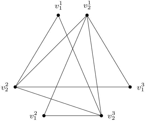
(a) $G_{2,3}^{1}$

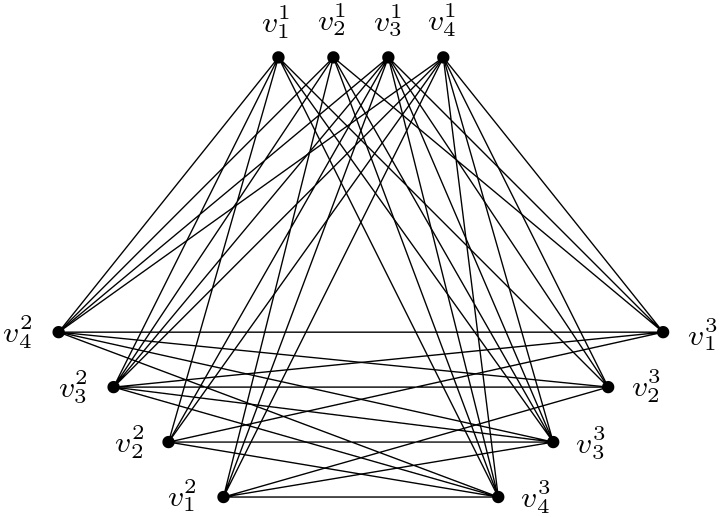
(b) $G_{4,3}^{2}$

Figure 2: Two examples of the graph $G_{k,\theta}^{d}$

The following proposition and its corollary show that the answer to Question 2 is no.

Proposition 4.7.

Let $k,\theta>1$ and fix $d$ such that $0\leq d\leq k$.

1. If $d=k$, then $G_{k,\theta}^{k}$ is isomorphic to $G_{\theta,k}^{\theta}$.

2. If either $d<k$, or $d=k$ and $k\geq\theta$, then the graph $G_{k,\theta}^{d}$ has coloring number $\theta$.

3. If $d<k$, then $G_{k,\theta}^{d}$ has exactly one proper $\theta$-coloring, up to a permutation of the coloring classes. This is given by $c\colon V\to\{1,\ldots,\theta\}$ such that $c(v)=i\iff v\in V_{i}$.

4. The graph $G_{k,\theta}^{d}$ satisfies

   $$e\bigl{(}v,V_{i}\bigr{)}=\begin{cases}\frac{\deg v}{\theta-1}&\text{ if }v\notin V_{i},\\ 0&\text{ if }v\in V_{i}.\end{cases}$$

5. If $0<d<k$, then $G_{k,\theta}^{d}$ has spectrum

   $$\Bigg{\{} \frac{k}{k-1}^{\bigl{(}d-1\bigr{)}},\frac{k^{2}-d}{k(k-1)}^{(1)},\frac{\theta}{\theta-1}^{\bigl{(}\theta-1\bigr{)}},1^{\bigl{(}(k-d-1)\theta\bigr{)}},$$

   $$\biggl{(}1-\frac{k-d}{k(k-1)(\theta-1)}\biggr{)}^{(\theta-1)},\biggl{(}1-\frac{1}{(k-1)(\theta-1)}\biggr{)}^{(d-1)(\theta-1)},0^{(1)}\Bigg{\}}.$$

6. If $d=k\geq\theta$ and $k\theta>4$, then $G_{k,\theta}^{d}$ has spectrum

   $$\Bigg{\{} \frac{\theta}{\theta-1}^{\bigl{(}\theta-1\bigr{)}},\frac{k}{k-1}^{\bigl{(}d-1\bigr{)}},\biggl{(}1-\frac{1}{(k-1)(\theta-1)}\biggr{)}^{(d-1)(\theta-1)},0^{(1)}\Bigg{\}}.$$

Proof.

1. It is easy to check that an isomorphism is given by

   $$V\Bigl{(}G_{k,\theta}^{k}\Bigr{)} \to V\Bigl{(}G_{\theta,k}^{\theta}\Bigr{)}$$

   $$v_{j}^{i} \mapsto v_{i}^{j}.$$

2. If $d<k$, then the coloring number of $G_{k,\theta}^{d}$ equals $\theta$ because the graph contains the $\theta$-clique $\{v_{d+1}^{1},\ldots,v_{d+1}^{\theta}\}$. Similarly, if $d=k$ and $k\geq\theta$, then the graph $G_{k,\theta}^{d}$ has coloring number $\theta$ since it contains the $\theta$-clique $\{v_{1}^{1},\ldots,v_{\theta}^{\theta}\}$.

3. Assume that $d<k$. Note that, for any proper coloring, for all $i$ such that $1\leq i\leq\theta$ we must have that the vertices $v_{d+1}^{i}$ have different colors, since they form a $\theta$-clique. Now let $c$ be a proper $\theta$-coloring such that $c\bigl{(}v_{d+1}^{i}\bigr{)}=i$, and fix $v_{j}^{i}\notin\{v_{d+1}^{1},\ldots,v_{d+1}^{\theta}\}$. Then, $v_{j}^{i}$ is adjacent to $v_{d+1}^{i^{\prime}}$ for $i^{\prime}\neq i$, implying that $c\bigl{(}v_{j}^{i}\bigr{)}=i$. This implies that there is one way to color $G_{k,\theta}^{d}$, up to permutation of the coloring classes.

4. This claim is true by construction.

5. We prove this claim by constructing linearly independent eigenfunctions for every eigenvalue.

   • For the eigenvalue $k/(k-1)$, we consider $d-1$ linearly independent functions $f_{1j}^{\prime}$ for $2\leq j\leq d$, defined by

     $$f_{1j}^{\prime}(v)=\begin{cases}1,&\text{ if }v=v_{1}^{i},1\leq i\leq\theta,\\ -1,&\text{ if }v=v_{j}^{i},1\leq i\leq\theta,\\ 0,&\text{ otherwise.}\end{cases}$$

     By Proposition 4.4, these are eigenfunctions corresponding to the eigenvalue $k/(k-1)$.

   • For the eigenvalue $(k^{2}-d)/(k(k-1))$, one can check that one eigenfunction is given by

     $$f(v)\coloneqq\begin{cases}-k(k-d),&\text{ if }v=v_{j}^{i},1\leq i\leq\theta,j\leq d,\\ d(k-1),&\text{ if }v=v_{j}^{i},1\leq i\leq\theta,j>d.\end{cases}$$

   • For the eigenvalue $\theta/(\theta-1)$, we have $\theta-1$ linearly independent eigenfunctions $f_{1i}$, for $2\leq i\leq\theta$, where $f_{1i}$ is defined as in Definition 2.10 with respect to the coloring classes $V_{i}$.

   • For the eigenvalue $1$, we have $(k-d-1)\theta$ linearly independent eigenfunctions $f_{v_{2}^{i},v_{j}^{i}}$ for $1\leq i\leq\theta$ and $d+2\leq j\leq k$, as in Definition 2.9:

     $$f_{v_{d+1}^{i},v_{j}^{i}}(v)\coloneqq\begin{cases}1,&\text{ if }v=v_{d+1}^{i},\\ -1,&\text{ if }v=v_{j}^{i},\\ 0,&\text{ otherwise.}\end{cases}$$

     One can check that these are eigenfunctions by observing that $v_{d+1}^{i}$ and $v_{j}^{i}$ are duplicate vertices if $j>d+1$, and by applying Proposition 4.4.

   • For the eigenvalue $1-(k-d)/(k(k-1)(\theta-1))$, we have $\theta-1$ linearly independent eigenfunctions $g_{1i}$ for $2\leq i\leq\theta$, defined by

     $$g_{1i}(v)\coloneqq\begin{cases}k(k-d),&\text{ if }v=v_{j}^{1},j\leq d,\\ -d(k-1),&\text{ if }v=v_{j}^{1},j>d,\\ -k(k-d),&\text{ if }v=v_{j}^{i},j\leq d,\\ d(k-1),&\text{ if }v=v_{j}^{i},j>d,\\ 0,&\text{ otherwise.}\end{cases}$$

   • For the eigenvalue $1-1/(k-1)(\theta-1)$, we have $(d-1)(\theta-1)$ linearly independent eigenfunctions $h_{ij}$, for $2\leq i\leq\theta$ and $2\leq j\leq d$, defined by

     $$h_{ij}(v):=\begin{cases}1,&\text{ if $v=v_{1}^{1}$ or $v=v_{j}^{i}$},\\ -1,&\text{ if $v=v_{j}^{1}$ or $v=v_{1}^{i}$},\\ 0,&\text{ otherwise.}\end{cases}$$

     One can check that these are eigenfunctions by applying Proposition 4.4.

6. The eigenfunctions in this case are given by the same functions as in point (v).∎

An immediate corollary is the following.

Corollary 4.8.

Let $k,\theta>1$ and $0<d\leq k$ such that $k,\theta$ and $d$ do not all equal $2$. Assume that $k\geq\theta$ if $d=k$. Then $G_{k,\theta}^{d}$ has coloring number $\theta$, and we have the following cases for its largest eigenvalue.

1. If $\theta<k$, then $G_{k,\theta}^{d}$ has largest eigenvalue $\theta/(\theta-1)$ with multiplicity $\theta-1$.

2. If $\theta=k$ and $d>1$, then $G_{k,\theta}^{d}$ has largest eigenvalue $\theta/(\theta-1)=k/(k-1)$ with multiplicity $\theta+d-2$.

3. If $\theta=k$ and $d=1$, then $G_{k,\theta}^{d}$ has largest eigenvalue $\theta/(\theta-1)$ with multiplicity $\theta-1$.

4. If $\theta=k+1$ and $d=1$, then $G_{k,\theta}^{d}$ has largest eigenvalue $\theta/(\theta-1)$ with multiplicity $\theta$.

5. If $\theta>k+1$ and $d=1$, then $G_{k,\theta}^{d}$ has largest eigenvalue $(k+1)/k>\theta/(\theta-1)$ with multiplicity $1$.

6. If $\theta>k>d>1$, then $G_{k,\theta}^{d}$ has largest eigenvalue $k/(k-1)>\theta/(\theta-1)$ with multiplicity $d-1$.

In particular, the first four cases in Corollary 4.8 give us graphs with largest eigenvalue $\chi/(\chi-1)$. The last two cases give us graphs for which Question 2 does not hold. Furthermore, the second case with $d<k$ and the fourth case give us graphs for which the converse of Proposition 3.7 is not true.

Note that the graphs $G_{k,\theta}^{d}$ that we constructed, and for which Question 2 does not hold, have coloring number $\chi\geq 4$. We leave it as an open question whether the answer to Question 2 is yes if $\chi=3$.

5 Constructing graphs with largest eigenvalue $\chi/(\chi-1)$

5.1 Preliminary definitions and results

Throughout this section, we fix two graphs $G_{1}$ and $G_{2}$, as well as vertices $x_{1}\in V(G_{1})$ and $x_{2}\in V(G_{2})$. We shall consider a graph operation, called the $1$-sum [18] or graph joining [2], which can applied to two graphs that have the same largest eigenvalue, to obtain a new graph with this same largest eigenvalue. In particular, we shall see that, if $G_{1}$ and $G_{2}$ have the same coloring number $\chi$ and largest eigenvalue

$$\lambda_{\max}(G_{1})=\lambda_{\max}(G_{2})=\frac{\chi}{\chi-1},$$

we can apply this operation to obtain a new graph with largest eigenvalue $\chi/(\chi-1)$. Furthermore, we shall give the multiplicity of the eigenvalue $\chi/(\chi-1)$ of the $1$-sum of $G_{1}$ and $G_{2}$ in terms of its multiplicity for $G_{1}$ and $G_{2}$.

We start by giving the definition of $1$-sum. The idea is that $G_{1}[x_{1}]\oplus G_{2}[x_{2}]$ is defined as the union of $G_{1}$ and $G_{2}$ in which the vertices $x_{1}$ and $x_{2}$ are identified in a new vertex $y$.

Definition 5.1.

The 1-sum $G_{1}[x_{1}]\oplus G_{2}[x_{2}]$ of $G_{1}$ and $G_{2}$ with respect to $x_{1}$ and $x_{2}$ is the graph defined by

$$V\biggl{(}G_{1}[x_{1}]\oplus G_{2}[x_{2}]\biggr{)} :=V(G_{1})\cup V(G_{2})\cup\{y\}\setminus\{x_{1},x_{2}\},$$

$$E\biggl{(}G_{1}[x_{1}]\oplus G_{2}[x_{2}]\biggr{)} :=E(G_{1})\cup E(G_{2})\cup\bigl{\{}\{y,v_{i}\}\colon\{v_{i},x_{i}\}\in E(G_{i}),i=1,2\bigr{\}}$$

$$\quad\setminus\bigl{\{}\{x_{i},v_{i}\}\colon v_{i}\in V(G_{i}),i=1,2\bigr{\}}.$$

Note that the $1$-sum depends on the choice of $x_{1}$ and $x_{2}$, as is illustrated in Figure 3. If every choice of $x_{1}$ results in the same graph $G_{1}[x_{1}]\oplus G_{2}[x_{2}]$, then we also use the notation $G_{1}\oplus G_{2}[x_{2}]$.

The definition of the $1$-sum of two graphs can be extended to the $1$-sum of $m$ graphs.

Definition 5.2.

For $1\leq i\leq m$, let $G_{i}$ be a graph and let $x_{i}\in V(G_{i})$. The $1$-sum of $G_{1},\ldots,G_{m}$ with respect to $x_{1},\ldots,x_{m}$, is the graph $\bigoplus_{i=1}^{m}G_{i}[x_{i}]$, defined by

$$V\biggl{(}\bigoplus_{i=1}^{m}G_{i}[x_{i}]\biggr{)} :=\bigcup_{i=1}^{m}V(G_{i})\cup\{y\}\setminus\{x_{i}\colon 1\leq i\leq m\},$$

$$E\biggl{(}\bigoplus_{i=1}^{m}G_{i}[x_{i}]\biggr{)} :=\bigcup_{i=1}^{m}V(G_{i})\cup\bigl{\{}\{y,v_{i}\}\colon\{v_{i},x_{i}\}\in E(G_{i}),1\leq i\leq m\bigr{\}}$$

$$\quad\setminus\bigl{\{}\{x_{i},v_{i}\}\colon v_{i}\in V(G_{i}),1\leq i\leq m\bigr{\}}.$$

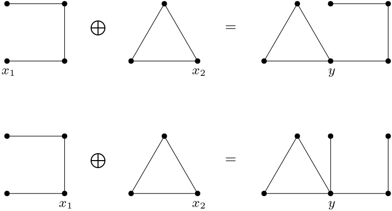
Figure 3: Two examples of the $1$-sum of two graphs with respect to $x_{1}$ and $x_{2}$

Remark 5.3.

In Definition 5.2, for the $1$-sum of $G_{1},\ldots,G_{m}$ we identify one vertex of each graph $G_{i}$ with the same vertex in $\bigoplus_{i=1}^{m}G_{i}[x_{i}]$.

Remark 5.4.

It can be easily seen that

$$\chi\bigl{(}G_{1}[x_{1}]\oplus G_{2}[x_{2}]\bigr{)}=\max\bigl{\{}\chi(G_{1}),\chi(G_{2})\bigr{\}}.$$

Another graph operation that we shall consider is the join.

Definition 5.5.

The join of $G_{1}$ and $G_{2}$, denoted $G_{1}\vee G_{2}$, is the graph constructed by taking the disjoint union of $G_{1}$ and $G_{2}$, and adding all edges between $V(G_{1})$ and $V(G_{2})$.

Example 5.6.

For $n\geq 2$, one can consider the $1$-sum $K_{n}^{(1)}\oplus K_{n}^{(2)}$ of two disjoint copies $K_{n}^{(1)}$ and $K_{n}^{(2)}$ of the complete graph on $n$ nodes. More generally, one can consider the $1$-sum of $m$ copies $K_{n}^{(i)}$ of $K_{n}$, denoted by

$$\bigoplus_{i=1}^{m}K_{n}^{(i)},$$

where we do not indicate with respect to what vertices $x_{i}$ we take the $1$-sum, as the choice of the vertices does not matter in this case. This gives one way of constructing the generalized petal graph (see Figure 4 for two examples), which can be equivalently defined as

$$K_{1}\vee mK_{n-1}.$$

As we shall see, defining the generalized petal graph as the $1$-sum of complete graphs, instead of the join of complete graphs, will allow us to infer that its largest eigenvalue must be $\chi/(\chi-1)=n/(n-1)$, and to compute its multiplicity, without having to calculate the whole spectrum. Furthermore, we shall generalize this result to the $1$-sum of arbitrary graphs.

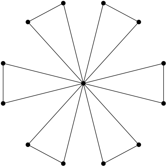
(a) The petal graph $\bigoplus_{i=1}^{6}K_{3}^{(i)}$

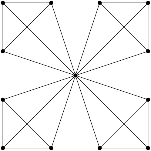
(b) The flying kite graph $\bigoplus_{i=1}^{4}K_{4}^{(i)}$

Figure 4: Two examples of generalized petal graphs

For the rest of this section, in addition to fixing $G_{1}$, $G_{2}$, $x_{1}\in V(G_{1})$ and $x_{2}\in V(G_{2})$, we also let $y$ be the vertex of $G_{1}[x_{1}]\oplus G_{2}[x_{2}]$ that is identified with $x_{1}$ and $x_{2}$. We identify the subgraph of $G_{1}[x_{1}]\oplus G_{2}[x_{2}]$ induced by $V(G_{1})\cup\{y\}\setminus\{x_{1}\}$ with $G_{1}$, and the subgraph induced by $V(G_{2})\cup\{y\}\setminus\{x_{2}\}$ with $G_{2}$.

We shall also need the following definition.

Definition 5.7.

Let $G^{\prime}$ be a subgraph of $G$. Given a function $f\colon V(G)\to\mathbb{R}$, its restriction to $G^{\prime}$ is defined as the function $f|_{G^{\prime}}\colon V(G^{\prime})\to\mathbb{R}$, given by $f|_{G^{\prime}}(v):=f(v)$ for all $v\in V(G^{\prime})$.

The following definition allows us to glue two functions together when taking the $1$-sum of two graphs.

Definition 5.8.

Let $f^{1}\colon V(G_{1})\to\mathbb{R}$ and $f^{2}\colon V(G_{2})\to\mathbb{R}$ be two functions such that $f^{1}(x_{1})=f^{2}(x_{2})$. Then we let

$$f^{1}\oplus_{x_{1},x_{2}}f^{2}\colon V(G_{1}[x_{1}]\oplus G_{2}[x_{2}])\to\mathbb{R}$$

be the function such that

$$\bigl{(}f^{1}\oplus_{x_{1},x_{2}}f^{2}\bigr{)}|_{G_{1}}=f^{1}\text{ and }\bigl{(}f^{1}\oplus_{x_{1},x_{2}}f^{2}\bigr{)}|_{G_{2}}=f^{2}.$$

Furthermore, for $i=1,2$, we fix the notation

$$\boldsymbol{0}^{i}\colon V(G_{i})\to\mathbb{R}$$

to denote the zero function.

We conclude with the following elementary lemma that will be needed in the proofs of this section.

Lemma 5.9.

Let $a,b,c,d\in\mathbb{R}_{>0}$. We have that

$$\frac{a+b}{c+d}\leq\max\biggl{\{}\frac{a}{c},\frac{b}{d}\biggr{\}}\quad\text{ and }\quad\frac{a+b}{c+d}\geq\min\biggl{\{}\frac{a}{c},\frac{b}{d}\biggr{\}}.$$

Moreover, equality holds if and only if $a/c=b/d$.

5.2 Spectral properties of the $1$-sum of graphs

In [2], Banerjee and Jost (2008) proved the following theorem.

Theorem 5.10 (Theorem 2.5 from [2]).

Assume that $\lambda$ is an eigenvalue of both $G_{1}$ and $G_{2}$, and that there exist corresponding eigenfunctions $f_{\lambda}^{1}$ and $f_{\lambda}^{2}$, such that $f_{\lambda}^{1}(p_{1})=f_{\lambda}^{2}(p_{2})=0$ for some $p_{1}\in V(G_{1})$ and $p_{2}\in V(G_{2})$. Then, the graph $G_{1}[p_{1}]\oplus G_{2}[p_{2}]$ also has eigenvalue $\lambda$, with an eigenfunction given by $f_{\lambda}^{1}\oplus_{p_{1},p_{2}}f_{\lambda}^{2}$.

Whereas we are interested in the largest eigenvalue of $G_{1}[x_{1}]\oplus G_{2}[x_{2}]$, Banerjee and Jost in [2] were mostly interested in constructing graphs which have eigenvalue $\lambda=1$. They observed that, if $G_{1}$ and $G_{2}$ both have eigenvalue $\lambda=1$ with corresponding eigenfunctions $f_{1}^{1}$ and $f_{1}^{2}$, then one only has to require that $f_{1}^{1}(x_{1})=f_{1}^{2}(x_{2})$, for $f_{1}^{1}\oplus_{x_{1},x_{2}}f_{1}^{2}$ to be an eigenfunction of $G_{1}[x_{1}]\oplus G_{2}[x_{2}]$. We now generalize this to arbitrary eigenvalues.

Proposition 5.11.

Assume that $G_{1}$ and $G_{2}$ have a common eigenvalue $\lambda$, and that there exist corresponding eigenfunctions $f^{i}(x_{i})\colon V(G_{i})\to\mathbb{R}$, for $i=1,2$, such that $f^{1}(x_{1})=f^{2}(x_{2})$. Then, $f^{1}\oplus_{x_{1},x_{2}}f^{2}$ is an eigenfunction for $G_{1}[x_{1}]\oplus G_{2}[x_{2}]$ with eigenvalue $\lambda$.

Proof.

Let $G\coloneqq G_{1}[x_{1}]\oplus G_{2}[x_{2}]$, $f\coloneqq f^{1}\oplus_{x_{1},x_{2}}f^{2}$ and $d_{i}\coloneqq\deg_{G_{i}}x_{i}$, for $i=1,2$. For $i=1,2$, and for every vertex $v_{i}\in V(G)\setminus\{y\}$ such that $v_{i}\in V(G_{i})$, we have that

$$(1-\lambda)f(v_{i}) =\frac{1}{\deg_{G_{i}}v_{i}}\left(\sum_{\begin{subarray}{c}w_{i}\in G_{i}\\ w_{i}\sim v_{i}\end{subarray}}f^{i}(w_{i})\right)=\frac{1}{\deg_{G}v_{i}}\left(\sum_{\begin{subarray}{c}w\in G\\ w\sim v_{i}\end{subarray}}f(w)\right).$$

Furthermore,

$$\frac{1}{\deg_{G}y}\Biggl{(}\sum_{\begin{subarray}{c}w\in G\\ w\sim y\end{subarray}}f(w)\Biggr{)} =\frac{d_{1}}{d_{1}+d_{2}}\cdot\frac{1}{d_{1}}\left(\sum_{\begin{subarray}{c}w_{1}\in G_{1}\\ w_{1}\sim x_{1}\end{subarray}}f(w_{1})\right)+\frac{d_{2}}{d_{1}+d_{2}}\cdot\frac{1}{d_{2}}\left(\sum_{\begin{subarray}{c}w_{2}\in G_{2}\\ w_{2}\sim x_{2}\end{subarray}}f(w_{2})\right)$$

$$=\frac{d_{1}}{d_{1}+d_{2}}(1-\lambda)f^{1}(x_{1})+\frac{d_{2}}{d_{1}+d_{2}}(1-\lambda)f^{2}(x_{2})$$

$$=(1-\lambda)f(y).$$

By (2), it follows that $f$ is an eigenfunction for $G$ with eigenvalue $\lambda$. ∎

We can also give a lower bound to the multiplicity of $\lambda$ as an eigenvalue of $G_{1}[x_{1}]\oplus G_{2}[x_{2}]$, as follows.

Theorem 5.12.

For every $\lambda\in[0,2]$, we have that

$$m_{G_{1}[x_{1}]\oplus G_{2}[x_{2}]}\bigl{(}\lambda\bigr{)}\geq m_{G_{1}}\bigl{(}\lambda\bigr{)}+m_{G_{2}}\bigl{(}\lambda\bigr{)}-1.$$

Proof.

For simplicity, let

$$m_{1} \coloneqq m_{G_{1}}\bigl{(}\lambda\bigr{)},$$

$$m_{2} \coloneqq m_{G_{2}}\bigl{(}\lambda\bigr{)},$$

$$m_{12} \coloneqq m_{G_{1}[x_{1}]\oplus G_{2}[x_{2}]}\bigl{(}\lambda\bigr{)}.$$

Furthermore, let

$$\bigl{\{}f^{1},g_{1}^{1},\ldots,g^{1}_{m_{1}-1}\bigr{\}}\quad\text{and}\quad\bigl{\{}f^{2},g_{1}^{2},\ldots,g^{2}_{m_{2}-1}\bigr{\}}$$

be (possibly empty) bases for the eigenspace of $\lambda$ as an eigenvalue of $G_{1}$ and $G_{2}$, respectively, such that $g^{1}_{i}(x_{1})=0=g^{2}_{j}(x_{2})$ for $1\leq i\leq m_{1}-1$ and $1\leq j\leq m_{2}-1$. Then, one can check that the functions

$$g^{1}_{i}\oplus_{x_{1},x_{2}}\boldsymbol{0}^{2}\quad\text{and}\quad\boldsymbol{0}^{1}\oplus_{x_{1},x_{2}}g^{2}_{j}$$

are $m_{1}+m_{2}-2$ linearly independent eigenfunctions of $G_{1}[x_{1}]\oplus G_{2}[x_{2}]$ with eigenvalue $\lambda$. Hence, if we construct one more eigenfunction, we are done. We consider two cases.

• $f^{1}(x_{1})=0$ or $f^{2}(x_{2})=0$. In this case, $f^{1}\oplus_{x_{1},x_{2}}\boldsymbol{0}^{2}$ or $\boldsymbol{0}^{1}\oplus_{x_{1},x_{2}}f^{2}$, respectively, is an eigenfunction of $G_{1}[x_{1}]\oplus G_{2}[x_{2}]$ with eigenvalue $\lambda$, and it is linearly independent from the $m_{1}+m_{2}-2$ eigenfunctions that we exhibited above.

• $f^{1}(x_{1})\neq 0$ and $f^{2}(x_{2})\neq 0$. In this case we can assume, without loss of generality, that $f^{1}(x_{1})=f^{2}(x_{2})$. By Proposition 5.11, the function $f^{1}\oplus_{x_{1},x_{2}}f^{2}$ is an eigenfunction for $G_{1}[x_{1}]\oplus G_{2}[x_{2}]$ with eigenvalue $\lambda$, and it is linearly independent from the $m_{1}+m_{2}-2$ eigenfunctions that we exhibited above.

This concludes the proof. ∎

Remark 5.13.

The inequality in Theorem 5.12 is not always an equality. To see this, consider the $m$-petal graph from Section 2.2, which can be seen as the $1$-sum of copies of $K_{3}$ (cf. Example 5.6). This graph has eigenvalue $1/2$, which is not an eigenvalue of $K_{3}$.

At the end of this section we shall compute the multiplicity of the eigenvalue

$$\lambda=\max\bigl{\{}\lambda_{\max}(G_{1}),\lambda_{\max}(G_{2})\bigr{\}}$$

for $G_{1}[x_{1}]\oplus G_{2}[x_{2}]$, by looking at eigenfunctions. This will be a consequence of the theorem below, which states that the largest eigenvalue of $G_{1}[x_{2}]\oplus G_{2}[x_{2}]$ is bounded above by the largest eigenvalues of both $G_{1}$ and $G_{2}$. This interlacing result complements the ones in [6] and, to the best of our knowledge, it has not been proved before.

Theorem 5.14.

We have that

$$\lambda_{\max}\bigl{(}G_{1}[x_{1}]\oplus G_{2}[x_{2}]\bigr{)}\leq\max\biggl{\{}\lambda_{\max}(G_{1}),\lambda_{\max}(G_{2})\biggr{\}}.$$ (12)

Proof.

Let $G$ denote $G_{1}[x_{1}]\oplus G_{2}[x_{2}]$ for simplicity. Let $f$ be such that $\textrm{RQ}(f)=\lambda_{\max}\bigl{(}G\bigr{)}$, and let $f^{i}\colon V_{i}\to\mathbb{R}$ be the restriction of $f$ to $G_{i}$, for $i=1,2$. If $f^{1}=\boldsymbol{0}^{1}$ , then the statement follows immediately, because in this case $\textrm{RQ}(f)=\textrm{RQ}(f^{2})$. If $f^{2}=\boldsymbol{0}^{2}$ , then the statement follows analogously. Otherwise, we can use Lemma 5.9 to infer that

$$\lambda_{\max}\bigl{(}G\bigr{)} =\textrm{RQ}(f)$$

$$=\frac{\sum_{\begin{subarray}{c}v,w\in V\bigl{(}G\bigr{)}\colon\\ v\sim w\end{subarray}}\biggl{(}f(v)-f(w)\biggr{)}^{2}}{\sum_{v\in V\bigl{(}G\bigr{)}}\deg_{G}vf(v)^{2}}$$

$$=\frac{\sum_{\begin{subarray}{c}v,w\in V(G_{1})\colon\\ v\sim w\end{subarray}}\biggl{(}f(v)-f(w)\biggr{)}^{2}+\sum_{\begin{subarray}{c}v,w\in V(G_{2})\colon\\ v\sim w\end{subarray}}\biggl{(}f(v)-f(w)\biggr{)}^{2}}{\sum_{v\in V(G_{1})}\deg_{G_{1}}vf(v)^{2}+\sum_{v\in V(G_{2})}\deg_{G_{2}}vf(v)^{2}}$$

$$\leq\max\left\{\frac{\sum_{\begin{subarray}{c}v,w\in V(G_{1})\colon\\ v\sim w\end{subarray}}\biggl{(}f(v)-f(w)\biggr{)}^{2}}{\sum_{v\in V(G_{1})}\deg_{G_{1}}vf(v)^{2}},\frac{\sum_{\begin{subarray}{c}v,w\in V(G_{2})\colon\\ v\sim w\end{subarray}}\biggl{(}f(v)-f(w)\biggr{)}^{2}}{\sum_{v\in V(G_{2})}\deg_{G_{2}}vf(v)^{2}}\right\}$$

$$=\max\{\textrm{RQ}(f^{1}),\textrm{RQ}(f^{2})\}$$

$$\leq\max\biggl{\{}\lambda_{\max}(G_{1}),\lambda_{\max}(G_{2})\biggr{\}}.\qed$$

The following is an immediate corollary of Theorem 5.14 and Theorem 3.1.

Corollary 5.15.

Let $G_{1}$ and $G_{2}$ be two graphs with the same coloring number $\chi$, such that $\lambda_{\max}(G_{1})=\lambda_{\max}(G_{2})=\chi/(\chi-1)$. Then,

$$\lambda_{\max}\bigl{(}G_{1}[x_{1}]\oplus G_{2}[x_{2}]\bigr{)}=\frac{\chi}{\chi-1}.$$

As a consequence of Corollary 5.15, given any two graphs with the same coloring number $\chi$ and with largest eigenvalue $\chi/(\chi-1)$, we can construct a new graph which also has coloring number $\chi$ (by Remark 5.4) and largest eigenvalue $\chi/(\chi-1)$, by taking their $1$-sum with respect to any pair of vertices.

The following theorem tells us when the inequality in Theorem 5.14 is an equality and, for this case, it also gives us the multiplicity of the largest eigenvalue.

Theorem 5.16.

If $\lambda_{\max}(G_{1})\geq\lambda_{\max}(G_{2})$, then

$$m_{G_{1}[x_{1}]\oplus G_{2}[x_{2}]}\bigl{(}\lambda_{\max}(G_{1})\bigr{)}\in$$

$$\quad\bigl{\{}m_{G_{1}}\bigl{(}\lambda_{\max}(G_{1})\bigr{)}+m_{G_{2}}\bigl{(}\lambda_{\max}(G_{2})\bigr{)},m_{G_{1}}\bigl{(}\lambda_{\max}(G_{1})\bigr{)}+m_{G_{2}}\bigl{(}\lambda_{\max}(G_{2})\bigr{)}-1\bigr{\}}.$$

More specifically, we have the following two cases.

1. Assume that, for $i=1,2$, for all $h_{i}\colon V(G_{i})\to\mathbb{R}$ such that $\textrm{RQ}_{G_{i}}(h_{i})=\lambda_{\max}(G_{i})$, we have that $h_{1}(x_{1})=0$ and $h_{2}(x_{2})=0$. In this case, we have that

   $$m_{G_{1}[x_{1}]\oplus G_{2}[x_{2}]}\bigl{(}\lambda_{\max}(G_{1})\bigr{)}=m_{G_{1}}\bigl{(}\lambda_{\max}(G_{1})\bigr{)}+m_{G_{2}}\bigl{(}\lambda_{\max}(G_{2})\bigr{)}.$$

2. Otherwise, we have that

   $$m_{G_{1}[x_{1}]\oplus G_{2}[x_{2}]}\bigl{(}\lambda_{\max}(G_{1})\bigr{)}=m_{G_{1}}\bigl{(}\lambda_{\max}(G_{1})\bigr{)}+m_{G_{2}}\bigl{(}\lambda_{\max}(G_{2})\bigr{)}-1.$$

Proof.

Let $G\coloneqq G_{1}[x_{1}]\oplus G_{2}[x_{2}]$, and let

$$m_{1} \coloneqq m_{G_{1}}\bigl{(}\lambda_{\max}(G_{1})\bigr{)},$$

$$m_{2} \coloneqq m_{G_{2}}\bigl{(}\lambda_{\max}(G_{2})\bigr{)},$$

$$m_{12} \coloneqq m_{G_{1}[x_{1}]\oplus G_{2}[x_{2}]}\bigl{(}\lambda_{\max}(G_{1})\bigr{)}.$$

Observe that, if $f\colon V(G)\to\mathbb{R}$ is an eigenfunction for $G$ with eigenvalue $\lambda_{\max}(G_{1})$, then exactly one of the following is true:

• $f|_{G_{1}}=\boldsymbol{0}^{1}$ and $\textrm{RQ}(f|_{G_{2}})=\lambda_{\max}(G_{1})$,

• $\textrm{RQ}(f|_{G_{1}})=\lambda_{\max}(G_{1})$ and $f|_{G_{2}}=\boldsymbol{0}^{2}$, or

• $\textrm{RQ}(f|_{G_{1}})=\lambda_{\max}(G_{1})$ and $\textrm{RQ}(f|_{G_{2}})=\lambda_{\max}(G_{1})$.

From the min-max Principle it follows that, for at least one $i\in\{1,2\}$, $f|_{G_{i}}$ is an eigenfunction for $G_{i}$ with eigenvalue $\lambda_{\max}(G_{i})$, and for at most one $i\in\{1,2\}$, $f|_{G_{i}}$ is the zero function on $G_{i}$. This allows us to give a basis for the eigenspace of $\lambda_{\max}(G_{1})$ for $G$, in terms of bases for the eigenspace of this eigenvalue for $G_{1}$ and $G_{2}$. As in the proof of Theorem 5.12, we let

$$\bigl{\{}f^{1},g_{1}^{1},\ldots,g^{1}_{m_{1}-1}\bigr{\}}\quad\text{and}\quad\bigl{\{}f^{2},g_{1}^{2},\ldots,g^{2}_{m_{2}-1}\bigr{\}}$$

denote (possibly empty) bases for the eigenspace of $\lambda_{\max}(G_{1})$ as an eigenvalue of $G_{1}$ and $G_{2}$, respectively, such that $g_{j}^{1}(x_{1})=0$ for $1\leq j\leq m_{1}-1$ and $g_{j}^{2}(x_{2})=0$ for $1\leq j\leq m_{2}-1$. We consider two cases.

1. If $f^{1}(x_{1})=0$ and $f^{2}(x_{2})=0$, then

   $$\bigl{\{}f^{1}\oplus_{x_{1},x_{2}}\boldsymbol{0}^{2},g^{1}_{1}\oplus_{x_{1},x_{2}}\boldsymbol{0}^{2},\ldots,g^{1}_{m_{1}-1}\oplus_{x_{1},x_{2}}\boldsymbol{0}^{2}\bigr{\}}\cup$$

   $$\bigl{\{}\boldsymbol{0}^{1}\oplus_{x_{1},x_{2}}f^{2},\boldsymbol{0}^{1}\oplus_{x_{1},x_{2}}g_{1}^{2},\ldots,\boldsymbol{0}^{1}\oplus_{x_{1},x_{2}}g^{2}_{m_{2}-1}\bigr{\}}$$

   is a basis for the eigenspace of the eigenvalue $\lambda_{\max}(G_{1})$ for $G$ of size $m_{1}+m_{2}$.

2. If one of $f^{1}(x_{1})$ and $f^{2}(x_{2})$ is non-zero, then we have one of the following three subcases.

   1. If $f^{1}(x_{1})=0$ and $f^{2}(x_{2})\neq 0$, then

      $$\bigl{\{}f^{1}\oplus_{x_{1},x_{2}}\boldsymbol{0}^{2},g^{1}_{1}\oplus_{x_{1},x_{2}}\boldsymbol{0}^{2},\ldots,g^{1}_{m_{1}-1}\oplus_{x_{1},x_{2}}\boldsymbol{0}^{2}\bigr{\}}\cup\bigl{\{}\boldsymbol{0}^{1}\oplus_{x_{1},x_{2}}g_{1}^{2},\ldots,\boldsymbol{0}^{1}\oplus_{x_{1},x_{2}}g^{2}_{m_{2}-1}\bigr{\}}$$

      is a basis for the eigenspace of $\lambda_{\max}(G_{1})$ for $G$ of size $m_{1}+m_{2}-1$.

   2. Analogously, if $f^{1}(x_{1})\neq 0$ and $f^{2}(x_{2})=0$, then

      $$\bigl{\{}g^{1}_{1}\oplus_{x_{1},x_{2}}\boldsymbol{0}^{2},\ldots,g^{1}_{m_{1}-1}\oplus_{x_{1},x_{2}}\boldsymbol{0}^{2}\bigr{\}}\cup\bigl{\{}\boldsymbol{0}^{1}\oplus_{x_{1},x_{2}}f^{2},\boldsymbol{0}^{1}\oplus_{x_{1},x_{2}}g_{1}^{2},\ldots,\boldsymbol{0}^{1}\oplus_{x_{1},x_{2}}g^{2}_{m_{2}-1}\bigr{\}}$$

      is a basis for the eigenspace of $\lambda_{\max}(G_{1})$ for $G$ of size $m_{1}+m_{2}-1$.

   3. If $f^{1}(x_{1})\neq 0$ and $f^{2}(x_{2})\neq 0$, then we assume that $f^{1}(x_{1})=f^{2}(x_{2})$, and we have that

      $$\bigl{\{}f^{1}\oplus_{x_{1},x_{2}}f^{2}\bigr{\}}\cup\bigl{\{}g^{1}_{1}\oplus_{x_{1},x_{2}}\boldsymbol{0}^{2},\ldots,g^{1}_{m_{1}-1}\oplus_{x_{1},x_{2}}\boldsymbol{0}^{2}\bigr{\}}\cup\bigl{\{}\boldsymbol{0}^{1}\oplus_{x_{1},x_{2}}g_{1}^{2},\ldots,\boldsymbol{0}^{1}\oplus_{x_{1},x_{2}}g^{2}_{m_{2}-1}\bigr{\}}$$

      is a basis for the eigenspace of $\lambda_{\max}(G_{1})$ for $G$ of size $m_{1}+m_{2}-1$.

   In all three subcases, we have that $m_{12}=m_{1}+m_{2}-1$.∎

As a corollary of Theorem 5.16, we can now give the multiplicity of the eigenvalue $\chi/(\chi-1)$ for the $1$-sum of two graphs that have coloring number $\chi$ and largest eigenvalue $\chi/(\chi-1)$.

Corollary 5.17.

Let $G_{1}$ and $G_{2}$ be graphs that have the same coloring number $\chi$ and largest eigenvalue

$$\lambda_{\max}(G_{1})=\lambda_{\max}(G_{2})=\frac{\chi}{\chi-1}.$$

Then, the multiplicity of the largest eigenvalue $\chi/(\chi-1)$ of $G_{1}[x_{1}]\oplus G_{2}[x_{2}]$ is

$$m_{G_{1}[x_{1}]\oplus G_{2}[x_{2}]}\biggl{(}\frac{\chi}{\chi-1}\biggr{)}=m_{G_{1}}\biggl{(}\frac{\chi}{\chi-1}\biggr{)}+m_{G_{2}}\biggl{(}\frac{\chi}{\chi-1}\biggr{)}-1.$$

Furthermore, the eigenfunctions corresponding to $\lambda_{\max}\bigl{(}G_{1}[x_{1}]\oplus G_{2}[x_{2}]\bigr{)}$ are precisely the non-zero functions $f$ such that $f|_{G_{1}}$ is either the zero function or an eigenfunction for $G_{1}$ with eigenvalue $\chi/(\chi-1)$, and $f|_{G_{2}}$ is either the zero function or an eigenfunction for $G_{2}$ with eigenvalue $\chi/(\chi-1)$.

Proof.

We are in the setting of Case (2)(iii) in the proof of Theorem 5.16, since we have that $f_{ij}^{1}\colon V(G_{1})\to\mathbb{R}$ from Definition 2.10 is non-zero on $x_{1}$, for $x_{1}\in V_{i}$, and we have that $f_{kl}^{2}\colon V(G_{2})\to\mathbb{R}$ is non-zero on $x_{2}$, for $x_{2}\in V_{k}$. This proves the first part of the corollary. The second part follows by looking at the basis that is given in Case (2)(iii) in the proof of Theorem 5.16. ∎

Example 5.18.

Consider the generalized petal graphs from Example 5.6. As a consequence of Corollary 5.17 we have that, for $n\geq 2$, the graph

$$G\coloneqq\bigoplus_{i=1}^{m}K_{n}^{(i)},$$

which has coloring number $\chi=n$, has largest eigenvalue

$$\lambda_{\max}(G)=\frac{\chi}{\chi-1}$$

with multiplicity $m(n-1)-m+1=|V(G)|-m$.

As two particular cases (for $m=1$ and $m=2$, respectively),

• The complete graph $K_{N}$ has largest eigenvalue $\chi/(\chi-1)$ with multiplicity $N-1$, and it is well-known that this is the only connected graph with an eigenvalue that has multiplicity $N-1$. Therefore, the complete graph is the only graph that has largest eigenvalue $\chi/(\chi-1)$ with multiplicity $N-1$.

• By Proposition 8 in [31], the generalized petal graph $K_{n}^{(1)}\oplus K_{n}^{(2)}$ is the only graph that has largest eigenvalue $\chi/(\chi-1)$ with multiplicity $N-2$.

Remark 5.19.

The $1$-sum of two complete graphs of the same size, $K_{n}^{(1)}\oplus K_{n}^{(2)}$, also has the property that its largest eigenvalue equals $(N+1)/(N-1)$. The only other graphs which have this property are complete graphs with one edge removed. All other non-complete graphs have largest eigenvalue strictly bigger than $(N+1)/(N-1)$, as proven by Sun and Das (2016) [26] and by Jost, Mulas and Münch (2021) [20].

5.3 Generalizing the $1$-sum

Different generalizations of the $1$-sum have been introduced in varying contexts. One of these is called the clique-sum, the $k$-clique-sum or the $k$-sum, depending on the reference, and it is used, for example, in the proof of the Structure Theorem from Robertson and Seymour (2003) [22] on the structure of graphs for which no minor is isomorphic to a fixed graph $H$. The idea of the $k$-clique-sum, for a positive integer $k$, is to first glue $G_{1}$ and $G_{2}$ together at a $k$-clique, and then remove either no, all or some of the edges of this $k$-clique in the new graph.

However, for the $k$-clique-sum,we cannot generalize Theorem 5.14. To see this, consider a $2$-clique-sum of two copies of $K_{3}$, both having largest eigenvalue $\lambda_{\max}(K_{3})=3/2$. In this case, the $2$-clique-sum can either be $C_{4}$ or $K_{4}\setminus\{e\}$ (depending on whether we remove the edge, i.e. the $2$-clique, in which we glue the graphs together). The former has largest eigenvalue $\lambda_{\max}(C_{4})=2$, and the latter has largest eigenvalue $\lambda_{\max}(K_{4}\setminus\{e\})=5/3$. Both these values are bigger than $\lambda_{\max}(K_{3})$. In Theorem 5.14 we saw, in contrast, that the opposite inequality is true for the $1$-sum.

The aim of this subsection is to offer a different generalization of the $1$-sum, for which we can prove a generalization of Theorem 5.14.

Definition 5.20.

Let $G_{1}$ and $G_{2}$ be graphs such that

$$E(G_{1})\cap E(G_{2})=\varnothing.$$

Their edge-disjoint union is the graph $G_{1}\sqcup_{E}G_{2}$ with vertex set

$$V(G_{1}\sqcup_{E}G_{2}):=V(G_{1})\cup V(G_{2})$$

and edge set

$$E(G_{1}\sqcup_{E}G_{2}):=E(G_{1})\sqcup E(G_{2}).$$

From here on, we fix two graphs $G_{1}$ and $G_{2}$ such that $E(G_{1})\cap E(G_{2})=\varnothing$.

Remark 5.21.

If $|V(G_{1})\cap V(G_{2})|=0$, then the edge-disjoint union of $G_{1}$ and $G_{2}$ is simply the disjoint union of $G_{1}$ and $G_{2}$. If $|V(G_{1})\cap V(G_{2})|=1$, then the edge-disjoint union and the $1$-sum of $G_{1}$ and $G_{2}$ coincide.

For the edge-disjoint union, we can prove the following generalization of Theorem 5.14.

Theorem 5.22.

We have that

$$\lambda_{\max}(G_{1}\sqcup_{E}G_{2})\leq\max\biggl{\{}\lambda_{\max}(G_{1}),\lambda_{\max}(G_{2})\biggr{\}}.$$

Proof.

The proof is analogous to the proof of Theorem 5.14. The key ingredients are Lemma 5.9 and the fact that $G_{1}$ and $G_{2}$ are edge-disjoint. ∎

An immediate corollary is the following.

Corollary 5.23.

Assume that $E_{1}\sqcup E_{2}=E(G)$, i.e., $E_{1}$ and $E_{2}$ form a partition of the edge set of $G$. For $i=1,2$, let $G_{i}$ be the graph with vertex set $V(G)$ and edge set $E_{i}$. Then,

$$\lambda_{\max}(G)\leq\max\biggl{\{}\lambda_{\max}(G_{1}),\lambda_{\max}(G_{2})\biggr{\}}.$$

Note that we cannot generalize the results from Section 5.2 about the $1$-sum and the coloring number to the more general case of the edge-disjoint union. This is partly due to the fact that the following inequality is not always an equality:

$$\chi(G_{1}\sqcup_{E}G_{2})\geq\max\{\chi(G_{1}),\chi(G_{2})\}.$$

However, we make the extra assumption that $\chi(G_{1}\sqcup_{E}G_{2})=\max\{\chi(G_{1}),\chi(G_{2})\}$, we can then generalize Corollary 5.15 to obtain the following corollary of Theorem 5.22 and Theorem 3.2.

Corollary 5.24.

If $G_{1}$ and $G_{2}$ are two graphs with the same coloring number $\chi$ such that $\lambda_{\max}(G_{1})=\lambda_{\max}(G_{2})=\chi/(\chi-1)$ and $\chi(G_{1}\sqcup_{E}G_{2})=\chi$, then

$$\lambda_{\max}\bigl{(}G_{1}\sqcup_{E}G_{2}\bigr{)}=\frac{\chi}{\chi-1}.$$

6 Upper bounds

In this section, we shall give some upper bounds on the largest eigenvalue $\lambda_{N}$ of a fixed graph $G$ which depend on its coloring number $\chi$. We start with a theorem for graphs that admit a proper $\chi$-coloring which has coloring classes of the same size, and we then generalize it to a theorem which applies to all graphs.

Theorem 6.1.

Let $\delta$ denote the smallest vertex degree of $G$. If there exists a proper $\chi$-coloring of the vertices for which all coloring classes have the same size, then

$$\lambda_{N}\leq\frac{N}{\delta}.$$

Moreover, the inequality is sharp.

Proof.

If $f$ is an eigenfunction for $\lambda_{N}$ and the coloring classes are denoted by $V_{1},\ldots,V_{\chi}$, then

$$\lambda_{N}(G) =\textrm{RQ}_{G}(f)$$

$$=\frac{\sum_{v\sim w}\biggl{(}f(v)-f(w)\biggr{)}^{2}}{\sum_{v\in V}\deg v\cdot f(v)^{2}}$$

$$=\frac{\sum_{i\neq j}\sum_{\begin{subarray}{c}w_{i}\sim w_{j},\\ w_{i}\in V_{i},w_{j}\in V_{j}\end{subarray}}\biggl{(}f(w_{i})-f(w_{j})\biggr{)}^{2}}{\sum_{v\in V}\deg v\cdot f(v)^{2}}$$

$$\leq\frac{\sum_{i\neq j}\sum_{\begin{subarray}{c}w_{i}\sim w_{j},\\ w_{i}\in V_{i},w_{j}\in V_{j}\end{subarray}}\biggl{(}f(w_{i})-f(w_{j})\biggr{)}^{2}}{\sum_{v\in V}\delta\cdot f(v)^{2}}$$

$$\leq\frac{\sum_{i\neq j}\sum_{w_{i}\in V_{i},w_{j}\in V_{j}}\biggl{(}f(w_{i})-f(w_{j})\biggr{)}^{2}}{\sum_{v\in V}\delta\cdot f(v)^{2}}.$$

Now, by assumption, each coloring class $V_{i}$ has size $N/\chi$. Let $\widehat{G}$ be the complete multipartite graph with partition classes $V_{1},\ldots,V_{\chi}$, and let $k:=N-N/\chi$. Then, $\widehat{G}$ is a $k$-regular graph and, by Theorem 3.6 in [27], $\lambda_{N}(\widehat{G})=\chi/(\chi-1)$. Therefore,

$$\lambda_{N}(G) \leq\frac{\sum_{i\neq j}\sum_{w_{i}\in V_{i},w_{j}\in V_{j}}\biggl{(}f(w_{i})-f(w_{j})\biggr{)}^{2}}{\sum_{v\in V}\delta\cdot f(v)^{2}}$$

$$=\frac{k}{\delta}\cdot\frac{\sum_{i\neq j}\sum_{w_{i}\in V_{i},w_{j}\in V_{j}}\biggl{(}f(w_{i})-f(w_{j})\biggr{)}^{2}}{\sum_{v\in V}k\cdot f(v)^{2}}$$

$$=\frac{k}{\delta}\cdot\textrm{RQ}_{\widehat{G}}(f)$$

$$\leq\frac{k}{\delta}\cdot\lambda_{N}(\widehat{G})$$

$$=\frac{k}{\delta}\cdot\frac{\chi}{\chi-1}$$

$$=\frac{N}{\delta}.$$

This proves the inequality. It is sharp since it becomes an equality for complete multipartite graphs with coloring classes of the same size. ∎

We now offer a generalization of Theorem 6.1 to all graphs.

Theorem 6.2.

Fix a proper $\chi$-coloring with coloring classes $V_{1},V_{2},\ldots,V_{\chi}$ such that their cardinalities $N_{i}\coloneqq|V_{i}|$ satisfy $N_{i}\geq N_{i+1}$ for $1\leq i\leq\chi$. Let also

$$x\coloneqq\min_{1\leq i\leq\chi,v\in V_{i}}\frac{\deg v}{N-N_{i}}.$$

Then,

$$\lambda_{N}\leq\frac{1}{x}\cdot\frac{N}{N-N_{1}}.$$

Furthermore, this inequality is sharp.

Proof.

If $f$ is an eigenfunction for $\lambda_{N}$, then

$$\lambda_{N}(G) =\textrm{RQ}_{G}(f)$$

$$=\frac{\sum_{v\sim w}\biggl{(}f(v)-f(w)\biggr{)}^{2}}{\sum_{v\in V}\deg v\cdot f(v)^{2}}$$

$$=\frac{\sum_{i\neq j}\sum_{\begin{subarray}{c}w_{i}\sim w_{j},\\ w_{i}\in V_{i},w_{j}\in V_{j}\end{subarray}}\biggl{(}f(w_{i})-f(w_{j})\biggr{)}^{2}}{\sum_{v\in V}\deg v\cdot f(v)^{2}}$$

$$\leq\frac{\sum_{i\neq j}\sum_{\begin{subarray}{c}w_{i}\sim w_{j},\\ w_{i}\in V_{i},w_{j}\in V_{j}\end{subarray}}\biggl{(}f(w_{i})-f(w_{j})\biggr{)}^{2}}{x\sum_{\begin{subarray}{c}1\leq i\leq\chi,\\ v\in V_{i}\end{subarray}}\bigl{(}N-N_{i}\bigr{)}f(v)^{2}}$$

$$\leq\frac{\sum_{i\neq j}\sum_{w_{i}\in V_{i},w_{j}\in V_{j}}\biggl{(}f(w_{i})-f(w_{j})\biggr{)}^{2}}{x\sum_{\begin{subarray}{c}1\leq i\leq\chi,\\ v\in V_{i}\end{subarray}}\bigl{(}N-N_{i}\bigr{)}f(v)^{2}}.$$

By assumption, each coloring class $V_{i}$ has size $N_{i}$. Let $\widehat{G}\coloneqq K_{N_{1},\ldots,N_{\chi}}$ be the complete multipartite graph with partition classes $V_{1},\ldots,V_{\chi}$. Then, by Theorem 3.5 in [28],

$$\lambda_{N}(\widehat{G})\leq\frac{N}{N-N_{1}}.$$

Therefore,

$$\lambda_{N}(G) \leq\frac{\sum_{i\neq j}\sum_{w_{i}\in V_{i},w_{j}\in V_{j}}\biggl{(}f(w_{i})-f(w_{j})\biggr{)}^{2}}{x\sum_{\begin{subarray}{c}1\leq i\leq\chi,\\ v\in V_{i}\end{subarray}}\bigl{(}N-N_{i}\bigr{)}f(v)^{2}}$$

$$=\frac{1}{x}\cdot\frac{\sum_{i\neq j}\sum_{w_{i}\in V_{i},w_{j}\in V_{j}}\biggl{(}f(w_{i})-f(w_{j})\biggr{)}^{2}}{\sum_{\begin{subarray}{c}1\leq i\leq\chi,\\ v\in V_{i}\end{subarray}}\bigl{(}N-N_{i}\bigr{)}f(v)^{2}}$$

$$=\frac{1}{x}\cdot\textrm{RQ}_{\widehat{G}}(f)$$

$$\leq\frac{1}{x}\cdot\lambda_{N}(\widehat{G})$$

$$\leq\frac{1}{x}\cdot\frac{N}{N-N_{1}}.$$

The inequality is sharp because of Theorem 6.1. ∎

We shall now prove a theorem for graphs that satisfy the setting of Question 2.

Theorem 6.3.

Fix a proper $\chi$-coloring that has coloring classes $V_{1},\ldots,V_{\chi}$. Assume that $G$ is $d$-regular, and that

$$e\bigl{(}v,V_{i}\bigr{)}=\begin{cases}\frac{\deg v}{\chi-1}&\text{ if }v\notin V_{i},\\ 0&\text{ if }v\in V_{i}.\end{cases}$$

Then,

$$\lambda_{N}\leq\max\biggl{\{}\frac{N}{d}\cdot\frac{\chi-1}{\chi},\frac{\chi}{\chi-1}\biggr{\}}.$$

Proof.

Let $f\notin\langle f_{1i}\colon 2\leq i\leq\chi\rangle$ be a non-constant function. Then, by Corollary 4.3, for all $j$ with $1\leq j\leq\chi$ we have that

$$\sum_{v\in V_{i}}f(v)=\frac{1}{d}\sum_{v\in V_{i}}\deg vf(v)=0.$$ (13)

This implies that

$$\textrm{RQ}(f) =\frac{\sum_{1\leq i<j\leq\chi}\sum_{\begin{subarray}{c}v_{i}\sim v_{j}\colon\\ v_{i}\in V_{i}\\ v_{j}\in V_{j}\end{subarray}}\Bigl{(}f(v_{i})-f(v_{j})\Bigr{)}^{2}}{d\sum_{v\in V}f(v)^{2}}$$

$$\leq\frac{\sum_{1\leq i<j\leq\chi}\sum_{\begin{subarray}{c}v_{i}\in V_{i}\\ v_{j}\in V_{j}\end{subarray}}\Bigl{(}f(v_{i})-f(v_{j})\Bigr{)}^{2}}{d\sum_{v\in V}f(v)^{2}}$$

$$=\frac{\sum_{v\in V}\Bigl{(}N-N/\chi\Bigr{)}f(v)^{2}-2\sum_{1\leq i<j\leq\chi}\sum_{v_{i}\in V_{i}}f(v_{i})\sum_{v_{j}\in V_{j}}f(v_{j})}{d\sum_{v\in V}f(v)^{2}}$$

$$\overset{\eqref{eq:sumzero}}{=}\frac{\Bigl{(}N-N/\chi\Bigr{)}\sum_{v\in V}f(v)^{2}}{d\sum_{v\in V}f(v)^{2}}$$

$$=\frac{N-N/\chi}{d}$$

$$=\frac{N}{d}\cdot\frac{\chi-1}{\chi}.$$

Furthermore, by Proposition 4.1, we have that the functions $f_{1i}$’s from Definition 2.10 are eigenfunctions with corresponding eigenvalue $\chi/(\chi-1)$. Therefore, if $f$ is an eigenfunction such that $\textrm{RQ}(f)=\lambda_{N}$, then either $\textrm{RQ}(f)=\chi/(\chi-1)$, or

$$\textrm{RQ}(f)>\frac{\chi}{(\chi-1)}\quad\text{and}\quad\textrm{RQ}(f)\leq\frac{N(\chi-1)}{d\chi}.$$

This implies that

$$\lambda_{N}\leq\max\biggl{\{}\frac{N}{d}\cdot\frac{\chi-1}{\chi},\frac{\chi}{\chi-1}\biggr{\}}.\qed$$

Remark 6.4.

Note that we cannot give a better upper bound than $2$ for $\lambda_{N}$ if our only information about a graph is its coloring number $\chi$. Consider, for example, the complete multipartite graph $G$ with coloring classes $V_{1},\ldots,V_{\chi}$ of sizes

$$|V_{i}|=\begin{cases}t,&\text{ if }i=1,\\ 1,&\text{ otherwise.}\end{cases}$$

This graph is also known as a complete split graph. Note that $N=|V(G)|=t+\chi-1$. We know by Lemma 2.14 in [24] that the largest eigenvalue of $G$ equals

$$\lambda_{N}(G)=1+\frac{t}{N-1}=2-\frac{\chi-2}{N-1}$$

and we have that

$$\lim_{N\to\infty}\lambda_{N}(G)=2-\lim_{N\to\infty}\biggl{(}\frac{\chi-2}{N-1}\biggr{)}=2.$$

Since we can choose $t$ independently of $\chi$, we see that the best upper bound that we can give for $\lambda_{N}$ equals $2$.

7 Open questions

We conclude by formulating some open questions.

The graphs $G_{k,\theta}^{d}$ that we constructed in Section 4, for which Question 2 does not hold, all have coloring numbers equal to at least $4$. Therefore, we may ask the following question:

Question 3.

Let $G$ be a graph with coloring number $\chi=3$ such that for any fixed proper $3$-coloring with coloring classes $V_{1},V_{2},V_{3}$ we have that

$$e(v,V_{i})=\begin{cases}\frac{\deg v}{2}&\text{ if }v\notin V_{i},\\ 0&\text{ if }v\in V_{i}.\end{cases}$$

Do we have that

$$\lambda_{N}=\frac{3}{2}?$$

In Example 5.18, we characterized graphs with largest eigenvalue $\chi/(\chi-1)$ whose multiplicity equals $N-1$ or $N-2$, respectively. Graphs with $\lambda_{N}=\chi/(\chi-1)$ whose multiplicity equals $N-3$ have also been characterized, and this result can be found in [29]. We may ask the following question:

Question 4.

Which graphs have largest eigenvalue $\chi/(\chi-1)$ with multiplicity $N-k$, where $k\geq 4$ is relatively small compared to $N$?

Disclosure statement

The authors report there are no competing interests to declare.

References

- [1] A. Abiad, R. Mulas, and D. Zhang. Coloring the normalized Laplacian for oriented hypergraphs. Linear Algebra and Its Applications, 629:192–207, 2021.
- [2] Anirban Banerjee and Jürgen Jost. On the spectrum of the normalized graph Laplacian. Linear Algebra Appl., 428(11-12):3015–3022, 2008.
- [3] L. W Beineke and R. J Wilson. Topics in chromatic graph theory, volume 156. Cambridge University Press, 2015.
- [4] B. Berlin and P. Kay. Basic color terms: Their universality and evolution. University of California Press, 1969.
- [5] A.E. Brouwer and W.H. Haemers. Spectra of graphs. Springer Science & Business Media, 2011.
- [6] S. Butler. Interlacing for weighted graphs using the normalized Laplacian. The Electronic Journal of Linear Algebra, 16:90–98, 2007.
- [7] S. Butler. Algebraic aspects of the normalized Laplacian. In Recent trends in combinatorics, volume 159 of IMA Vol. Math. Appl., pages 295–315. Springer, [Cham], 2016.
- [8] S. Butler and F. Chung. Spectral graph theory. In Handbook of linear algebra. Florida: CRC Press, 2006.
- [9] M. Cavers. The normalized Laplacian matrix and general Randic index of graphs. ProQuest LLC, Ann Arbor, MI, 2010. Thesis (Ph.D.)–The University of Regina (Canada).
- [10] G. Chartrand and P. Zhang. Chromatic graph theory. Discrete Mathematics and its Applications (Boca Raton). CRC Press, Boca Raton, FL, 2009.
- [11] H. Chen and L. Liao. The normalized Laplacian spectra of the corona and edge corona of two graphs. Linear Multilinear Algebra, 65(3):582–592, 2017.
- [12] F. Chung. Spectral graph theory. American Mathematical Soc., 1997.
- [13] G. Coutinho, R. Grandsire, and C. Passos. Colouring the normalized Laplacian. Electronic Notes in Theoretical Computer Science, 346:345–354, 2019.
- [14] D Cvetkovic. Spectral theory of graphs based on the signless laplacian. Technical report, Research report, 2010.
- [15] D. Cvetković, P. Rowlinson, and S. Simić. An introduction to the theory of graph spectra, volume 75 of London Mathematical Society Student Texts. Cambridge University Press, Cambridge, 2010.
- [16] Z. Füredi. Turán type problems. Surveys in combinatorics, 166:253–300, 1991.
- [17] C. Godsil and G. Royle. Algebraic graph theory, volume 207 of Graduate Texts in Mathematics. Springer-Verlag, New York, 2001.
- [18] F. Gurski. The behavior of clique-width under graph operations and graph transformations. Theory Comput. Syst., 60(2):346–376, 2017.
- [19] A. J. Hoffman. On eigenvalues and colorings of graphs. In Graph Theory and its Applications (Proc. Advanced Sem., Math. Research Center, Univ. of Wisconsin, Madison, Wis., 1969), pages 79–91. Academic Press, New York-London, 1970.
- [20] J. Jost, R. Mulas, and F. Münch. Spectral gap of the largest eigenvalue of the normalized graph Laplacian. Communications in Mathematics and Statistics, 2021.
- [21] J. Jost, R. Mulas, and D. Zhang. Petals and books: the largest Laplacian spectral gap from 1. J. Graph Theory, 104(4):727–756, 2023.
- [22] N. Robertson and P. D. Seymour. Graph minors. XVI. Excluding a non-planar graph. J. Combin. Theory Ser. B, 89(1):43–76, 2003.
- [23] A. Sidorenko. What we know and what we do not know about Turán numbers. Graphs and Combinatorics, 11(2):179–199, 1995.
- [24] S. Sun and K. C. Das. On the second largest normalized Laplacian eigenvalue of graphs. Appl. Math. Comput., 348:531–541, 2019.
- [25] S. Sun and K. C. Das. On the multiplicities of normalized Laplacian eigenvalues of graphs. Linear Algebra Appl., 609:365–385, 2021.
- [26] S. Sun and K.C. Das. Extremal graph on normalized laplacian spectral radius and energy. The Electronic Journal of Linear Algebra, 29:237–253, 2016.
- [27] S. Sun and K.C. Das. Normalized Laplacian eigenvalues with chromatic number and independence number of graphs. Linear and Multilinear Algebra, 68(1):63–80, 2020.
- [28] S. Sun and K.C. Das. Normalized Laplacian spectrum of complete multipartite graphs. Discrete Appl. Math., 284:234–245, 2020.
- [29] F. Tian and Y. Wang. Full characterization of graphs having certain normalized Laplacian eigenvalue of multiplicity . Linear Algebra Appl., 630:69–83, 2021.
- [30] P. Turán. On an extremal problem in graph theory (in Hungarian). Mat. Fiz. Lapok, 48:436–452, 1941.
- [31] E. R. van Dam and G. R. Omidi. Graphs whose normalized Laplacian has three eigenvalues. Linear Algebra Appl., 435(10):2560–2569, 2011.
- [32] P. Wocjan and C. Elphick. New spectral bounds on the chromatic number encompassing all eigenvalues of the adjacency matrix. Electron. J. Combin., 20(3):39, 18, 2013.