Joint and Robust Beamforming Framework for Integrated Sensing and Communication Systems

Abstract

Integrated sensing and communication (ISAC) is widely recognized as a fundamental enabler for future wireless communications. In this paper, we present a joint communication and radar beamforming framework for maximizing a sum spectral efficiency (SE) while guaranteeing desired radar performance with imperfect channel state information (CSI) in multi-user and multi-target ISAC systems. To this end, we adopt either a radar transmit beam mean square error (MSE) or receive signal-to-clutter-plus-noise ratio (SCNR) as a radar performance constraint of a sum SE maximization problem. To resolve inherent challenges such as non-convexity and imperfect CSI, we reformulate the problems and identify first-order optimality conditions for the joint radar and communication beamformer. Turning the condition to a nonlinear eigenvalue problem with eigenvector dependency (NEPv), we develop an alternating method which finds the joint beamformer through power iteration and a Lagrangian multiplier through binary search. The proposed framework encompasses both the radar metrics and is robust to channel estimation error with low complexity. Simulations validate the proposed methods. In particular, we observe that the MSE and SCNR constraints exhibit complementary performance depending on the operating environment, which manifests the importance of the proposed comprehensive and robust optimization framework.

I Introduction

The upcoming era of wireless communication networks is poised to accommodate substantial data transmission speeds, top-notch wireless connectivity for a multitude of devices, and remarkably precise and resilient sensing capabilities [1, 2]. Motivated by this, the concept of integrated sensing and communication (ISAC), which unifies signal processing techniques and hardware infrastructure between sensing and communication systems, is widely acknowledged as a pivotal technology for the realization of future wireless networks [3, 4]. The integration of radar and communications on a unified platform holds the potential to reduce platform costs, facilitate spectrum sharing, and enhance performance through the synergy between radar and communications. Perceiving these promising advantages, we investigate a multiple-input and multiple-output (MIMO) ISAC system and propose a novel MIMO-ISAC beamforming framework.

I-A Related Works

In early studies, a system in which a separately located radar base station (BS) and cellular BS share spectrum with cooperation was mainly considered. In [5], a simple opportunistic spectrum sharing method was proposed by exploiting radar rotation information, showing the potential of radar-communication coexistence. Assuming the similar setup to [5], in [6], a power control method was developed and it was revealed that the power control allows very short spatial separation between the radar and communication BSs. Considering a MIMO radar system, a null space projection approach was proposed in [7] for minimizing a negative impact of a radar signal to communication systems. Incorporating the impact of the reflected radar signal from clutters, a beamforming optimization problem was tackled in [8]. In this work, the importance of considering the channel estimation error was demonstrated from simulations. In [9], a robust MIMO beamforming technique was developed to cope with the imperfect knowledge on channel state information at a transmitter (CSIT) for coexistence of a radar and a cellular BS.

Despite the benefits obtained from the coexistence of radar and communication, simply sharing the spectrum with separated locations has fundamental limitations. That is to say, a significant amount of overheads is caused in exchanging information between radar and cellular infrastructures for cooperation. To overcome this, not only sharing the spectrum, but also unifying infrastructures of radar and communication has drawn significant attentions; leading to the emergence of an integrated sensing and communication (ISAC) system [10, 11, 12, 13, 14]. Nonetheless, several challenges newly have arisen for realizing the ISAC system, mainly caused by the difference between the primary goals of the two different applications [14].

To resolve the difficulties in realizing the unified system, extensive investigation has been performed for the ISAC system design. In [15], it studied the sensing performance of various waveform including orthogonal frequency-division multiplexing (OFDM) and direct sequence spread spectrum and showed that OFDM offers many advantages regarding the performance of the radar application. Information-theoretical approaches for analyzing and designing the unified system were also proposed by integrating not only the hardware infrastructure but also the performance metrics of the sensing and the communications [16, 17]. Using the unified information-theoretical radar and communication performance metrics, transmit waveform design was tackled in [18].

The aforementioned ISAC studies [15, 19, 16, 18, 20] mainly assumed a single-antenna system. An essential issue for achieving high efficiency in ISAC systems is forming multiple beams carefully by considering multiple communication users and radar targets; which propelled the use of a MIMO-ISAC system. In [21], an information embedding technique wherein communication signals are conveyed into MIMO radar beams by controlling their side-lobes was proposed assuming a line-of-sight channel. In addition, index-modulation type transmission schemes for delivering communication signals through MIMO radar waveform were proposed in [22, 23, 24, 25].

For MIMO-ISAC systems, ISAC transmit beamforming optimization has been actively explored in the literature. In [26, 27], joint beamforming optimization methods were proposed. The key idea is employing the manifold optimization technique, by which the mean squared error (MSE) between the desired beampattern and the current beampattern is minimized while satisfying a power constraint. In [26, 27], communication symbols are used not only for downlink user service, but also for radar target sensing; yet this is sub-optimal compared to a case that uses designated radar sensing symbols [28]. Addressing this limitation, in [29], a joint beamforming optimization framework was proposed for a MIMO-ISAC system wherein radar sensing symbols are designated. A similar problem was also considered in [28], assuming that each communication user is cable of eliminating radar sensing signals. In [30], a fairness-profile optimization problem was addressed for joint precoding and radar signaling, in which a difference between peak and side lobe of radar beams is controlled with communication signal-to-interference-plus-noise ratio (SINR) constraints. In [31], a sum rate maximization problem was formulated with radar transmit beam at target direction as a penalty term and solved by alternating methods. Considering a dirty paper coding scheme, joint ISAC beamforming problems were also tackled in [32] by leveraging the uplink-downlink duality.

Beyond conventional downlink setups, various scenarios of ISAC systems has also been explored recently. Incorporating a concept of physical layer security into a MIMO-ISAC system, secure transmission methods were proposed in [33, 34]. Employing advanced multiple access technique such as rate-splitting multiple access (RSMA) or non-orthognal multiple access (NOMA) into a MIMO-ISAC system, RSMA-based MIMO-ISAC system [35] and NOMA-based MIMO-ISAC system [36] were investigated.

Previous research endeavors on ISAC systems have adeptly elucidated the merits of integrating these systems while furnishing cutting-edge optimization techniques aimed at enhancing both radar and communication performance [29, 31]. These investigations have identified that a shared-antenna ISAC system surpasses its separate-antenna counterpart, and underscored the desirability of leveraging dedicated radar signals to fully exploit the available spatial degrees of freedom (DoF). Consequently, the development of ISAC beamforming strategies tailored to shared-antenna systems with designated radar signals, especially under realistic scenarios such as imperfect CSIT, multiple users, and multiple targets, is regarded as a pertinent research imperative; yet it has not been completely addressed. For instance, in [33, 34], robust transmission strategies using imperfect CSIT were proposed, primarily targeting scenarios involving a single target or a single user, respectively. There exist some prior works that considered multi-user scenarios [31, 29] and multi-target settings [29]; yet they predominantly assumed perfect CSIT. In response to this research gap, we propose a comprehensive framework for joint and robust beamforming optimization, harnessing dedicated radar signals in the shared-antenna ISAC systems that support multiple users and cater to multiple targets under the assumption of the imperfect CSIT.

I-B Contributions

In this paper, we propose a robust and joint beamforming optimization framework for MIMO-ISAC systems to maximize the sum spectral efficiency (SE) while achieving the desired radar performances. The proposed framework is designed for multi-user and multi-target scenarios, and comprehensive radar metrics with designated radar signals under the imperfect CSIT assumption. Our main contributions are summarized as:

• We formulate two communication-oriented ISAC beamforming problems, each of which considers distinct radar metrics: radar transmit beam MSE and radar receive signal-to-clutter-plus-noise ratio (SCNR). These problems involve maximizing the sum SE subject to either the MSE or the SCNR constraint, by which our problem incorporates the transmit and receive perspectives of radar probing signals, respectively. However, due to the non-convex nature of these optimization problems and the presence of the imperfect CSIT, addressing these problems are challenging. To resolve the challenge, we propose a joint beamforming optimization framework. Our method is featured by 1) capability of accommodating both radar metrics (the MSE and the SCNR), 2) robustness against the imperfect CSIT, and 3) efficiency in achieving strong communication and sensing performances.

• To this end, we first reformulate the problems by deriving a lower bound on the average SE in terms of the channel estimation error. This reformulation allows us to leverage the channel estimation error covariance in optimization. Then we obtain a tractable form of the problems by representing the objective function and constraints as a function of a vectorized joint communication and radar beamformer. Subsequently, we compute the Lagrangian function of each problem and derive a stationarity condition of the Karush–Kuhn–Tucker (KKT) condition with respect to the vectorized beamformer to identify local optimal points for a given Lagrangian multiplier.

• In pursuit of finding the best stationary point that maximizes the Lagrangian function, we interpret the obtained stationarity condition as a nonlinear eigenvalue problem with eigenvector dependency (NEPv). In the NEPv, the eigenvector and eigenvalue correspond to the vectorized beamformer and Lagrangian, respectively. This observation indicates that the principal eigenvector of the NEPv is equivalent to the best stationary point. Accordingly, for the given Lagrangian multiplier, we propose a generalized power iteration (GPI)-based algorithm to find the principal eigenvector. Given the beamforming vector, a binary search-based algorithm is used to update a proper Lagrangian multiplier that meets the radar constraint. The beamforming vector and the Lagrangian multiplier are updated in an alternating manner until convergence. As a special case, we also put forth radar-only beam design algorithms by using our proposed framework.

• Through simulations, we demonstrate that the proposed algorithms outperform other benchmark algorithms by offering a better trade-off between radar and communication performance and more robust performance under the imperfect CSIT. In addition to the performance gains, our method also sheds lights on crucial design guidelines for MIMO-ISAC, that could not be extracted through existing methods. For example, it becomes evident that careful selection of the radar metrics is desirable: the considered radar metrics exhibit a complementary relationship to each other depending on the operating environment. This observation underpins the importance of the proposed comprehensive optimization framework.

Notation: a is a scalar, ${\bf{a}}$ is a vector and ${\bf{A}}$ is a matrix. Superscripts $(\cdot)^{\sf T}$, $(\cdot)^{\sf H}$, and $(\cdot)^{-1}$ are matrix transpose, Hermitian, and inversion, respectively. $\mathbb{E}[\cdot]$ and $\text{tr}(\cdot)$ represent expectation operation and trace of a matrix, respectively. ${\bf{I}}_{N}$ is an $N\times N$ identity matrix. ${\bf 0}_{N\times M}$ is the $N\times M$ zero matrix. We denote $\otimes$ as kronecker product, and ${\bf e}^{N}_{n}$ as an $N\times 1$ standard basis vector whose $n$th element is one. ${\rm diag}({\bf a})$ is a diagonal matrix with ${\bf a}$ on its diagonal elements. $\mathcal{CN}(m,\sigma^{2})$ is a complex Gaussian distribution with mean $m$ and variance $\sigma^{2}$.

II System Model

II-A Signal Model

We consider a MIMO-ISAC system, where the BS equipped with a ISAC transmitter and a radar receiver operating on a single-hardware platform with $N$ transmit and receive antennas performs two disparate functions: 1) serving $K$ single antenna communication users and 2) forming radar beams for sensing potential targets. We refer to this BS as ISAC-BS. These two functionalities simultaneously share time-frequency resources and transmit antenna arrays. As assumed in [20], we consider complete decoupling between transmit and receive antennas, ensuring that the radar receiver remains free from self-interference when operating in full-duplex radar mode thanks to self-interference mitigation methods [37, 38]. To maximally exploit the spatial DoF provided by the MIMO system, the BS uses dedicated radar signals by superimposing them with communication symbols. Accordingly, the BS transmits the signal ${\bf{x}}\in\mathbb{C}^{N}$ defined as

$${\bf{x}}={\bf{F}}_{\text{C}}{\bf{s}}_{\text{C}}+{\bf{F}}_{\text{R}}{\bf{s}}_{\text{R}}=[{\bf{F}}_{\text{C}},{\bf{F}}_{\text{R}}]\left[{\bf{s}}_{\text{C}}^{\sf T},{\bf{s}}_{\text{R}}^{\sf T}\right]^{\sf T}={\bf{F}}{\bf{s}},$$ (1)

where ${\bf{s}}_{\text{R}}=[s_{{\rm R},1},\dots,s_{{\rm R},K}]^{\sf T}\in\mathbb{C}^{M}$ is a radar waveform signal vector, ${\bf{F}}_{\text{R}}=\left[{\bf{f}}_{{\text{R}},1},\cdots,{\bf{f}}_{{\text{R}},M}\right]\in\mathbb{C}^{N\times M}$ is a radar beamforming matrix, ${\bf{s}}_{\text{C}}=[s_{{\rm C},1},\dots,s_{{\rm C},K}]^{\sf T}\in\mathbb{C}^{K}$ is a communication message symbol vector, and ${\bf{F}}_{\text{C}}=\left[{\bf{f}}_{{\text{C}},1},\cdots,{\bf{f}}_{{\text{C}},K}\right]\in\mathbb{C}^{N\times K}$ is a communication beamforming matrix.

We further assume that the radar waveform signal ${\bf{s}}_{\text{R}}$ and the communication symbols ${\bf{s}}_{\text{C}}$ are zero-mean and statistically independent to each other, i.e., $\mathbb{E}\left[{\bf{s}}_{\text{R}}{\bf{s}}_{\text{C}}^{\sf H}\right]={\bf{0}}_{M\times K}$, with $\mathbb{E}\left[{\bf{s}}_{\text{R}}{\bf{s}}_{\text{R}}^{\sf H}\right]=P\cdot{\bf{I}}_{M}$, and $\mathbb{E}\left[{\bf{s}}_{\text{C}}{\bf{s}}_{\text{C}}^{\sf H}\right]=P\cdot{\bf{I}}_{K}$, where $P$ is the transmit power. Fulfilling a transmit power constraint, we assume $\|{\bf{F}}_{\text{R}}\|_{\sf F}+\|{\bf{F}}_{\text{C}}\|_{\sf F}\leq 1$ without loss of generality.

II-B Channel Model

The received signal $y_{k}$ received at user $k$ is given by

$$y_{k} ={\bf{h}}_{k}^{\sf H}{\bf{f}}_{{\text{C}},k}{\bf{s}}_{{\text{C}},k}\!+\!\sum_{i\neq k,i=1}^{K}{\bf{h}}_{k}^{\sf H}{\bf{f}}_{{\text{C}},i}{\bf{s}}_{{\text{C}},i}\!+\!\sum_{j=1}^{M}{\bf{h}}_{k}^{\sf H}{\bf{f}}_{{\text{R}},j}{\bf{s}}_{{\text{R}},j}\!+\!n_{k},$$ (2)

where ${\bf{h}}_{k}\in\mathbb{C}^{N}$ is the channel vector from the BS and user $k$, and $n_{k}\sim\mathcal{CN}(0,\sigma^{2})$ is the additive white Gaussian noise (AWGN). In (2), the second term indicates the aggregated interference from other communication users’ signals, and third term is the aggregated interference from the radar-sensing waveform signals.

For each channel vector, we assume ${\bf{h}}_{k}\sim\mathcal{CN}({\bf 0}_{K\times 1},{\bf{K}}_{k})$, i.e., it is distributed as Gaussian with a specific spatial covariance matrix ${\bf{K}}_{k}$. Upon this channel model, ${\bf{h}}_{k}$ is given as

$${\bf{h}}_{k}={\bf{U}}_{k}{\bf\Lambda}_{k}^{\frac{1}{2}}{\tilde{\bf{h}}}_{k},$$ (3)

where ${\bf\Lambda}_{k}\in\mathbb{C}^{r_{k}\times r_{k}}$ is a diagonal matrix that contains the non-zero eigenvalues of ${\bf{K}}_{k}$, ${\bf{U}}_{k}\in\mathbb{C}^{N\times r_{k}}$ is a collection of the eigenvectors of ${\bf{K}}_{k}$ corresponding to ${\bf\Lambda}_{k}$, and $\tilde{\bf{h}}_{k}\in\mathbb{C}^{r_{k}}$ is a independent and identically distributed (IID) channel vector whose element is drawn from $\mathcal{CN}(0,1)$. We note that our channel model encompasses most of the widely-used spatially correlated MIMO channel models.

For imperfect CSIT, the estimated CSIT is modeld as

$$\hat{\bf{h}}_{k}={\bf{h}}_{k}-{\boldsymbol{\phi}}_{k},$$ (4)

where ${\boldsymbol{\phi}}_{k}$ is the CSIT estimation error vector. We assume that $\hat{\bf{h}}_{k}$ and ${\boldsymbol{\phi}}_{k}$ are Gaussian-distributed and independent to each other. The error covariance is defined as ${\bf{\Phi}}_{k}=\mathbb{E}[{\boldsymbol{\phi}}_{k}{\boldsymbol{\phi}}^{\sf{H}}_{k}]$. We assume that the BS has the knowledge of $\hat{\bf{h}}_{k}$ and ${\bf{\Phi}}_{k}$.

II-C Radar Model

In many instances, successful sensing necessitates a direct line-of-sight (LoS) between the sensor and the target object. In conventional radar applications, signals bouncing off non-target objects are known as clutter. Unlike the communication systems which take advantage of the multiple paths of channels, the clutter is considered detrimental for sensing accuracy and requires mitigation. Involving the clutter, the received radar echo signal is modeled as [14]

$${\bf y}_{\rm R} =\sum_{i=1}^{S}\beta_{i}^{\rm tar}{\bf a}_{\rm r}(\theta^{\rm tar}_{i}){\bf a}_{\rm t}^{\sf H}(\theta^{\rm tar}_{i}){\bf x}+\sum_{j=1}^{C}\beta_{j}^{\rm cl}{\bf a}_{\rm r}(\theta^{\rm cl}_{j}){\bf a}_{\rm t}^{\sf H}(\theta^{\rm cl}_{j}){\bf x}+{\bf n}_{\rm R}$$

$$={\bf G}_{\rm tar}{\bf x}+{\bf G}_{\rm cl}{\bf x}+{\bf n}_{\rm R},$$ (5)

where $S$ is the number of targets, $C$ is the number of clutters, ${\bf a}_{\rm t}(\theta)$ is the transmitter array response vector to the direction $\theta$, ${\bf a}_{\rm r}(\theta)$ is the receiver array response vector to the direction $\theta$, $\theta^{\rm tar}_{i}$ is the direction of the $i$th target, $\theta^{\rm cl}_{j}$ is the direction of the $j$th clutter, $\beta_{i}^{\rm tar}$ is the reflection coefficient of the $i$th target, $\beta_{j}^{\rm cl}$ is the reflection coefficient of the $j$th clutter, and ${\bf n}_{\rm R}\sim\mathcal{CN}({\bf 0}_{N\times 1},\sigma^{2}_{\rm R}{\bf I}_{N})$ is the AWGN vector. Here ${\bf G}_{\rm tar}=\sum_{i=1}^{S}\beta_{i}^{\rm tar}{\bf a}_{\rm r}(\theta^{\rm tar}_{i}){\bf a}_{\rm t}^{\sf H}(\theta^{\rm tar}_{i})$ and ${\bf G}_{\rm cl}=\sum_{j=1}^{C}\beta_{j}^{\rm cl}{\bf a}_{\rm r}(\theta^{\rm cl}_{j}){\bf a}_{\rm t}^{\sf H}(\theta^{\rm cl}_{j})$. We consider that the reflection coefficients of the targets and clutters and the directions of clutters and reflection coefficients are known at the BS since they are large-scale parameters. In addition, when the clutters are fixed, e.g. buildings, light poles, trees, etc., $\theta_{j}^{\rm cl}$ and $\beta_{j}^{\rm cl}$ are almost time-invariant. We remark that the considered model can be regarded as a narrowband system or a subcarrier of an OFDM system.

II-D Performance Metrics and Problem Formulation

II-D1 Communication Performance Metric

We use a sum SE as a performance metric. The SINR at user $k$ is given as

$$\gamma_{k}=\frac{\left|{\bf{h}}_{k}^{\sf H}{\bf{f}}_{{\text{C}},k}\right|^{2}}{\sum_{i\neq k,i=1}^{K}\left|{\bf{h}}_{k}^{\sf H}{\bf{f}}_{{\text{C}},i}\right|^{2}+\sum_{j=1}^{M}\left|{\bf{h}}_{k}^{\sf H}{\bf{f}}_{{\text{R}},j}\right|^{2}+\frac{\sigma^{2}}{P}}.$$ (6)

In (6), we observe that the interference includes both i) the inter-user interference and ii) the radar waveform interference. The SE achieved at user $k$ is presented as

$$R_{k}=\log_{2}\left(1+\gamma_{k}\right).$$ (7)

II-D2 Radar Performance Metric

We consider two radar performance metrics: radar transmit beam pattern MSE and radar receive SCNR, and formulate problems with each metric.

Mean Squared Error (MSE): As in the prior works [28, 26, 29], the MSE between the transmit beam pattern and the desired beam pattern is often considered as a key radar performance metric. Specifically, assuming that the ISAC-BS operates in a narrowband and the propagation paths to radar sensing targets are LoS, the baseband signal at $\theta$ is

$$z(\theta)={\bf{a}}_{\rm t}^{\sf H}(\theta){\bf{x}}.$$ (8)

We note that the ISAC-BS is able to exploit not only the radar waveform signals ${\bf{s}}_{\rm R}$, but also the communication signals ${\bf{s}}_{\rm C}$ in forming radar sensing beam patterns. With (8), the radar beam power for an angular direction $\theta$ is characterized as

$$B({\bf F};\theta) =\mathbb{E}\left[|z(\theta)|^{2}\right]=P\cdot{\bf{a}}_{\rm t}^{\sf H}(\theta){\bf{F}}{\bf{F}}^{\sf H}{\bf{a}}_{\rm t}(\theta).$$ (9)

Now we define the MSE between the formed beam patterns and the given desired beam patterns as follows:

$${\text{MSE}}_{\text{R}}({\bf F})=\frac{1}{L}\sum_{\ell=1}^{L}|P\cdot d(\theta_{\ell})-B({\bf F};\theta_{\ell})|^{2},$$ (10)

where is $d(\theta)$ is the given normalized desired transmit beam mask for the direction $\theta$, and $L$ is the number of sampled angular grids. As ${\text{MSE}}_{\text{R}}$ decreases, the actual radar beam patterns become similar to the desired beam patterns. Accordingly, the advantage of using ${\text{MSE}}_{\text{R}}$ as a radar performance metric is that the transmit beam pattern can be directly designed to match the desired beam pattern. In this regard, it is particularly useful to design beams with multiple target angles.

Signal-to-Clutter-plus-Noise Ratio (SCNR): The limitation of using ${\text{MSE}}_{\text{R}}$ (10) is that it is hard to incorporate the effect of the undesirable echo signals, i.e., clutters. To resolve this problem, the SCNR can be used as a radar performance metric when clutters are non-negligible. For instance, the SCNR metric can be effective for a radar tracking phase in which the expected target positions and clutter positions are available. From (5), the SCNR is computed as [39, 14]

$$\gamma_{\rm R}({\bf F})\!=\!\frac{\mathbb{E}[\|{\bf G}_{\rm tar}{\bf x}\|_{\sf F}]}{\mathbb{E}[\|{\bf G}_{\rm cl}{\bf x}\|_{\sf F}\!+\!\|{\bf n}_{\rm R}\|_{\sf F}]}\!=\!\frac{{\rm Tr}\left({\bf G}_{\rm tar}{\bf F}{\bf F}^{\sf H}{\bf G}_{\rm tar}^{\sf H}\right)}{{\rm Tr}\left({\bf G}_{\rm cl}{\bf F}{\bf F}^{\sf H}{\bf G}_{\rm cl}^{\sf H}\right)\!+\!\frac{N}{P}\sigma^{2}_{\rm R}}.$$ (11)

Using the SCNR in (11) allows to take into account the effect of the clutters, whereas direct beam pattern design cannot be performed, which is different from using the MSE. Consequently, beam patterns for multiple targets may not be suitable with the SCNR as it considers the sum power from all targets, not individual power. Therefore, the MSE and SCNR can be viewed as complementary to each other.

II-D3 Problem Formulation

Considering communication-oriented ISAC systems, our main design goal is to maximize the sum SE under a constraint that the radar beam pattern MSE is smaller than the predefined threshold $T_{\rm mse}$:

$$\mathop{\text{maximize}}_{{\bf{F}}}\;\; R_{\Sigma}({\bf F})=\sum_{k=1}^{K}R_{k}({\bf F})$$ (12)

subjectto $${\rm MSE}_{\rm R}({\bf F})\leq T_{\rm mse},$$ (13)

$${\rm Tr}({\bf F}{\bf F}^{\sf H})\leq 1,$$ (14)

where (14) indicates the transmit power constraint. Similarly, with the SCNR performance metric, we formulate the problem:

$$\mathop{\text{maximize}}_{{\bf{F}}}\;\; R_{\Sigma}({\bf F})=\sum_{k=1}^{K}R_{k}({\bf F})$$ (15)

subjectto $$\gamma_{\rm R}({\bf F})\geq T_{\rm scnr},$$ (16)

$${\rm Tr}({\bf F}{\bf F}^{\sf H})\leq 1.$$ (17)

The problems are non-convex, and due to the assumption of the imperfect CSIT, the sum SE $R_{\Sigma}$ needs to be handled to fully utilize the estimated channel and error covariance matrix.

III Proposed Optimization Framework

In this section, we put forth our unified framework to solve (12) and (15). We first reformulate the objective function and constraints into tractable forms. Leveraging the reformulation, we study the first-order optimality condition, and then develop an efficient algorithm to find the maximum local optimal point. We first show the proposed framework for the problem in (12), and then apply it to solve the problem in (15).

III-A Problem Reformulation with MSE Constraint

We recall that the BS is only able to use the estimated CSIT $\hat{\bf{h}}_{k}$ and its error covariance matrix ${\bf\Phi}_{k}$. Accordingly, it is necessary to obtain a proper SE expression instead of $R_{\Sigma}({\bf F})$. To this end, we consider the average SE in terms of the CSIT estimation error [40] which is computed as

$$\bar{R}_{k}({\bf F})=\mathbb{E}_{\boldsymbol{\phi}_{k}}[R_{k}({\bf F})]$$ (18)

$$\!\!\!=\!\mathbb{E}_{{\boldsymbol{\phi}}_{k}}\!\!\left[\log_{2}\left(\!1\!+\!\frac{\left|\left(\hat{\bf{h}}_{k}\!+\!{\boldsymbol{\phi}}_{k}\right)^{\sf H}{\bf{f}}_{{\text{C}},k}\right|^{2}}{\sum_{i\neq k}^{K}\!\left|\left(\hat{\bf{h}}_{k}\!+\!{\boldsymbol{\phi}}_{k}\right)^{\sf H}\!\!\!{\bf{f}}_{{\text{C}},i}\right|^{2}\!\!\!+\!\sum_{j=1}^{M}\!\left|\left(\hat{\bf{h}}_{k}\!+\!{\boldsymbol{\phi}}_{k}\right)^{\sf H}\!\!\!{\bf{f}}_{{\text{C}},j}\right|^{2}\!\!\!+\!\frac{\sigma^{2}}{P}}\!\right)\right].$$

To convert (18) into a tractable closed form, we first rewrite the signal model (2) with the CSIT estimation error term as

$$y_{k} =\hat{\bf{h}}_{k}^{\sf H}{\bf{f}}_{{\text{C}},k}{{s}}_{{\text{C}},k}+\sum_{i\neq k,i=1}^{K}\hat{\bf{h}}_{k}^{\sf H}{\bf{f}}_{{\text{C}},i}{{s}}_{{\text{C}},i}+\sum_{j=1}^{M}\hat{\bf{h}}_{k}^{\sf H}{\bf{f}}_{{\text{R}},j}{{s}}_{{\text{R}},j}$$

$$\quad+\underbrace{\sum_{i^{\prime}=1}^{K}{\boldsymbol{\phi}}_{k}^{\sf H}{\bf{f}}_{{\text{C}},i^{\prime}}{{s}}_{{\text{C}},i^{\prime}}+\sum_{j^{\prime}=1}^{M}{\boldsymbol{\phi}}_{k}^{\sf H}{\bf{f}}_{{\text{R}},j^{\prime}}{{s}}_{{\text{R}},j^{\prime}}}_{(a)}+n_{k}.$$ (19)

We observe that the term $(a)$ entails several randomness associated with ${\boldsymbol{\phi}}_{k}$, ${\bf{s}}_{{\text{C}}}$, and ${\bf{s}}_{{\text{R}}}$. Although $(a)$ is correlated with the desired signal term due to ${\bf{s}}_{{\text{C}},k}$, we remove the correlation by treating $(a)$ as an independent Gaussian interference. This assumption leads to a lower bound of the SE $R_{k}$ by following a concept of generalized mutual information [41]. Then we have the following lower bound of (18) as shown in (22) at the top of the next page,

$$\bar{R}_{k}({\bf F}) \geq\mathbb{E}_{{\boldsymbol{\phi}}_{k}}\left[\log_{2}\left(1+\frac{\left|\hat{\bf{h}}_{k}^{\sf H}{\bf{f}}_{{\text{C}},k}\right|^{2}}{\sum_{i\neq k,i=1}^{K}\left|\hat{\bf{h}}_{k}^{\sf H}{\bf{f}}_{{\text{C}},i}\right|^{2}+\sum_{j=1}^{M}\left|\hat{\bf{h}}_{k}^{\sf H}{\bf{f}}_{{\text{R}},j}\right|^{2}+\sum_{i^{\prime}=1}^{K}\left|{\boldsymbol{\phi}}_{k}^{\sf H}{\bf{f}}_{{\text{C}},i^{\prime}}\right|^{2}+\sum_{j^{\prime}=1}^{M}\left|{\boldsymbol{\phi}}_{k}^{\sf H}{\bf{f}}_{{\text{R}},j^{\prime}}\right|^{2}+\frac{\sigma^{2}}{P}}\right)\right]$$ (20)

$$\mathop{\geq}^{(b)}\log_{2}\left(1+\frac{\left|\hat{\bf{h}}_{k}^{\sf H}{\bf{f}}_{{\text{C}},k}\right|^{2}}{\sum_{i\neq k,i=1}^{K}\left|\hat{\bf{h}}_{k}^{\sf H}{\bf{f}}_{{\text{C}},i}\right|^{2}+\sum_{j=1}^{M}\left|\hat{\bf{h}}_{k}^{\sf H}{\bf{f}}_{{\text{R}},j}\right|^{2}+\sum_{i^{\prime}=1}^{K}{\bf{f}}_{{\text{C}},i^{\prime}}^{\sf H}{\bf{\Phi}}_{k}{\bf{f}}_{{\text{C}},i^{\prime}}+\sum_{j^{\prime}=1}^{M}{\bf{f}}_{{\text{R}},j^{\prime}}^{\sf H}{\bf{\Phi}}_{k}{\bf{f}}_{{\text{R}},j^{\prime}}+\frac{\sigma^{2}}{P}}\right)$$ (21)

$$=\bar{R}_{k}^{\sf lb}({\bf F}).$$ (22)

 

where $(b)$ follows from Jensen’s inequality and $\mathbb{E}[{\boldsymbol{\phi}}_{k}{\boldsymbol{\phi}}_{k}^{\sf H}]={\bf{\Phi}}_{k}$. Since $\bar{R}_{k}^{{\sf{lb}}}$ is derived as a closed form, we use this as a new objective function in our optimization problem. Furthermore, $\bar{R}_{k}^{\sf lb}$ is a function of $\hat{\bf{h}}_{k}$ and ${\bf{\Phi}}_{k}$ that are available at the BS; thereby $\bar{R}_{k}^{\sf lb}$ can be fully used to design the beamforming matrix at the BS side.

Let us denote $\bar{\bf{f}}={\text{vec}}({\bf{F}})\in\mathbb{C}^{N(K+M)}$, i.e., the vectorized beamforming variable, and assume $\|\bar{\bf{f}}\|^{2}=1$ which implies signaling with maximum transmit power $P$. Since the sum SE increases with the transmit power, this assumption aligns with the problem in maximizing the sum SE. Then, we further reformulate $\bar{R}_{k}^{\sf lb}$ for more tractability as

$$\bar{R}_{k}^{\sf lb}(\bar{\bf f})=\log_{2}\left(\frac{\bar{\bf{f}}^{\sf H}{\bf{B}}_{k}\bar{\bf{f}}}{\bar{\bf{f}}^{\sf H}{\bf{C}}_{k}\bar{\bf{f}}}\right),$$ (23)

where ${\bf{B}}_{k}={\bf I}_{(K+M)}\otimes\big{(}\hat{\bf{h}}_{k}\hat{\bf{h}}_{k}^{\sf H}\!+\!{\bf{\Phi}}_{k}\big{)}\!+\!\frac{\sigma^{2}}{P}{\bf{I}}_{N(K+M)}$ and ${\bf{C}}_{k}={\bf{B}}_{k}-{\rm diag}\left({\bf e}^{(K+M)}_{k}\right)\otimes\hat{\bf{h}}_{k}\hat{\bf{h}}_{k}^{\sf H}.$

The next step is to reformulate the MSE constraint as a function of ${\bar{\bf f}}$. The radar beam power in (9) is rewritten as

$$B({\bf F};\theta) =P\cdot{\bf{a}}_{\rm t}^{\sf H}(\theta){\bf{F}}{\bf{F}}^{\sf H}{\bf{a}}_{\rm t}(\theta)$$ (24)

$$=P\cdot{\text{vec}}\left({\bf{a}}_{\rm t}^{\sf H}(\theta){\bf{F}}{\bf{F}}^{\sf H}{\bf{a}}_{\rm t}(\theta)\right)$$ (25)

$$\mathop{=}^{(a)}P\cdot\left(\left({\bf{a}}_{\rm t}^{\sf T}(\theta){\bf{F}}^{*}\right)\otimes{\bf{a}}_{\rm t}^{\sf H}(\theta)\right){\text{vec}}({\bf{F}})$$ (26)

$$\mathop{=}^{(b)}P\cdot\left(\left(\left({\bf{I}}\otimes{\bf{a}}_{\rm t}^{\sf T}(\theta)\right){\text{vec}}({\bf{F}}^{*})\right)^{\sf T}\otimes{\bf{a}}_{\rm t}^{\sf H}(\theta)\right){\text{vec}}({\bf{F}})$$

$$\mathop{=}\bar{\bf{f}}^{\sf H}\left(P\cdot{\bf{I}}\otimes{\bf{a}}_{\rm t}(\theta)\otimes{\bf{a}}_{\rm t}^{\sf H}(\theta)\right)\bar{\bf{f}},$$ (27)

where $(a)$ and $(b)$ follow from ${\text{vec}}({\bf{ABC}})=({\bf{C}}^{\sf T}\otimes{\bf{A}}){\text{vec}}({\bf{B}})$. Let us define ${\bf{A}}(\theta)=P\cdot{\bf{I}}\otimes{\bf{a}}_{\rm t}(\theta)\otimes{\bf{a}}_{\rm t}^{\sf H}(\theta)$. Then, the MSE of the radar beam pattern becomes

$${\text{MSE}}_{\text{R}}({\bf F})=\frac{1}{L}\sum_{\ell=1}^{L}|Pd(\theta_{\ell})-\bar{\bf{f}}^{\sf H}{\bf{A}}(\theta_{\ell})\bar{\bf{f}}|^{2}.$$ (28)

Assuming full power transmission, i.e., $\|\bar{\bf{f}}\|^{2}=1$, (28) is further rewritten as

$${\text{MSE}}_{\text{R}}({\bf F})=\frac{1}{L}{\sum_{\ell=1}^{L}|\bar{\bf{f}}^{\sf H}{\bf{D}}(\theta_{\ell})\bar{\bf{f}}-\bar{\bf{f}}^{\sf H}{\bf{A}}(\theta_{\ell})\bar{\bf{f}}|^{2}},$$ (29)

where ${\bf{D}}(\theta_{\ell})=P\cdot d(\theta_{\ell})\cdot{\bf{I}}_{N(K+M)}$.

Lastly, we relax the problem by omitting the power constraint ${\rm Tr}({\bf FF}^{\sf H})=\|\bar{\bf{f}}\|^{2}=1$ and consider it back in the algorithm to obtain the solution within the feasible set. Applying (23) and (29) to the problem in (12), our main problem is reformulated as

$$\mathop{\text{maximize}}_{\bar{\bf{f}}}\;\; \bar{R}_{\Sigma}^{\rm lb}(\bar{\bf f})=\sum_{k=1}^{K}\bar{R}_{k}^{\rm lb}(\bar{\bf f})$$ (30)

subjectto $$\frac{1}{L}\sum_{\ell=1}^{L}|\bar{\bf{f}}^{\sf H}{\bf{D}}(\theta_{\ell})\bar{\bf{f}}-\bar{\bf{f}}^{\sf H}{\bf{A}}(\theta_{\ell})\bar{\bf{f}}|^{2}\leq T_{\rm mse}.$$ (31)

We remark that this reformulated problem is still non-convex. Accordingly, it is NP-hard to find a global optimal solution, and instead, we show how to obtain a good local optimal solution of the reformulated and relaxed problem (30).

III-B Proposed Algorithm with MSE Constraint

To identify a local optimal solution, we study the first-order optimality condition; we derive the stationarity condition of the KKT condition for (30) in the following lemma:

Lemma 1.

The KKT stationarity condition of the problem in (30) is satisfied if the following condition holds:

$${\bf{\Psi}}(\bar{\bf{f}})\bar{\bf{f}}={\bf{\Omega}}(\bar{\bf{f}})\lambda(\bar{\bf{f}})\bar{\bf{f}},$$ (32)

where

$${\bf{\Psi}}(\bar{\bf{f}})=\lambda_{\sf num}(\bar{\bf{f}})\left[\sum_{k=1}^{K}\frac{{\bf{B}}_{k}}{\bar{\bf{f}}^{\sf H}{\bf{B}}_{k}\bar{\bf{f}}}+\right.$$ (33)

$$\left.\qquad\frac{2\mu\log 2}{LP^{2}}\sum_{\ell=1}^{L}\left\{(\bar{\bf{f}}^{\sf H}{\bf{D}}(\theta_{\ell})\bar{\bf{f}}){\bf{A}}(\theta_{\ell})+(\bar{\bf{f}}^{\sf H}{\bf{A}}(\theta_{\ell})\bar{\bf{f}}){\bf{D}}(\theta_{\ell})\right\}\right],$$

$${\bf{\Omega}}(\bar{\bf{f}})=\lambda_{\sf den}(\bar{\bf{f}})\left[\sum_{k=1}^{K}\frac{{\bf{C}}_{k}}{\bar{\bf{f}}^{\sf H}{\bf{C}}_{k}\bar{\bf{f}}}+\right.$$ (34)

$$\left.\qquad\frac{2\mu\log 2}{LP^{2}}\sum_{\ell=1}^{L}\left\{(\bar{\bf{f}}^{\sf H}{\bf{D}}(\theta_{\ell})\bar{\bf{f}}){\bf{D}}(\theta_{\ell})+(\bar{\bf{f}}^{\sf H}{\bf{A}}(\theta_{\ell})\bar{\bf{f}}){\bf{A}}(\theta_{\ell})\right\}\right].$$

Here, $\mu$ in (33) and (34) is the Lagrangian multiplier and

$$\lambda(\bar{\bf{f}}) =\prod_{k=1}^{K}\left(\frac{\bar{\bf{f}}^{\sf H}{\bf{B}}_{k}\bar{\bf{f}}}{\bar{\bf{f}}^{\sf H}{\bf{C}}_{k}\bar{\bf{f}}}\right)2^{\mu\left(\frac{T_{\rm mse}}{P^{2}}-\frac{1}{LP^{2}}\sum_{\ell=1}^{L}|\bar{\bf{f}}^{\sf H}{\bf{D}}(\theta_{\ell})\bar{\bf{f}}-\bar{\bf{f}}^{\sf H}{\bf{A}}(\theta_{\ell})\bar{\bf{f}}|^{2}\right)}$$ (35)

$$=\frac{\lambda_{\sf num}(\bar{\bf{f}})}{\lambda_{\sf den}(\bar{\bf{f}})},$$ (36)

where $\lambda_{\sf num}(\bar{\bf{f}})$ and $\lambda_{\sf den}(\bar{\bf{f}})$ are any functions that satisfy (36).

Proof.

See Appendix A. ∎

If the problem in (30) is convex, we can reach a global optimal point by jointly finding the Lagrangian multiplier $\mu$ and $\bar{\bf f}$ by solving the KKT condition including the stationarity condition in (32). Since our problem is non-convex, however, it is infeasible to find a global optimal point with the derived condition, and only a necessary condition of the local optimal point is guaranteed. In addition, the Lagrangian multiplier $\mu$ and the optimization variable $\bar{\bf{f}}$ are complicatedly intertwined, making it challenging to jointly optimize $\mu$ and $\bar{\bf{f}}$ even for the local optimal point. To resolve this difficulty, we alternately optimize $\mu$ adn $\bar{\bf{f}}$ by using Lemma 1. To this end, we have the following interpretation of the condition in (32):

III-B1 Interpretation

We know that if a precoding vector $\bar{\bf{f}}$ satisfies (32), then it satisfies the stationarity condition. Although the condition can be met with such a stationary point $\bar{\bf f}$, this point cannot guarantee an efficient solution since it can be a random local optimal point due to the non-convexity of (30). To achieve an efficient solution, we first explain how the objective function $\bar{R}_{\Sigma}^{\sf lb}(\bar{\bf f})$ in (30) and $\lambda(\bar{\bf f})$ in (32) are related. Let us assume that we have any precoder and Lagrangian multiplier pair $(\bar{\bf f}^{\dagger},\mu^{\dagger})$ that satisfies the MSE constraint (31) with equality and the stationarity condition $\eqref{eq:lemma_kkt}$, i.e., $(\bar{\bf f}^{\dagger},\mu^{\dagger})$ meets the necessary condition of the local maximum point. In such a case, because of the active MSE constraint, we have $\log_{2}\lambda(\bar{\bf f}^{\dagger})=R_{\Sigma}^{\sf lb}(\bar{\bf f}^{\dagger})$ which is a local maximum from the stationarity condition. This suggest that we need to find such $(\bar{\bf f}^{\dagger},\mu^{\dagger})$ that maximizes $\lambda(\bar{\bf f}^{\dagger})$ among stationary points.

To find a good stationary point that maximizes $\lambda(\bar{\bf f}^{\dagger})$, we see (32) through lens of functional eigenvalue problems. Since ${\bf\Omega}(\bar{\bf f})$ is invertible, we can represent the condition in (32) as

$${\bf{\Omega}}^{-1}(\bar{\bf{f}}){\bf{\Psi}}(\bar{\bf{f}})\bar{\bf{f}}=\lambda(\bar{\bf{f}})\bar{\bf{f}}.$$ (37)

Interpreting $\bar{\bf{f}}$ as an eigenvector and $\lambda(\bar{\bf{f}})$ as a corresponding eigenvalue of ${\bf{\Omega}}^{-1}(\bar{\bf{f}}){\bf{\Psi}}(\bar{\bf{f}})$, the KKT stationarity condition (32) is equivalent to a functional eigenvalue problem. More rigorously, (32) is cast as a NEPv [42]. As described in [42], NEPv is a generalized version of an eigenvector problem, in that a corresponding matrix is changed depending on an eigenvector in a non-linear fashion. Recall that we need to find $(\bar{\bf f}^{\dagger},\mu^{\dagger})$ which maximizes $\lambda(\bar{\bf f}^{\dagger})$ to maximize the objective function among the stationary points. To this end, we should derive the principal eigenvector of (37), $\bar{\bf f}^{\star}$, with corresponding $\mu^{\star}$ that keeps the MSE constraint active, thereby maximizing $\lambda(\bar{\bf f})$ among the stationary points. Then such point $\bar{\bf f}^{\star}$ is likely to be the best local optimal point. This observation is summarized in the following proposition:

Proposition 1.

Consider that $\bar{\bf{f}}^{\star}$ is the principal eigenvector of ${\bf{\Omega}}^{-1}(\bar{\bf{f}}^{\star}){\bf{\Psi}}(\bar{\bf{f}}^{\star})$ satisfying

$${\bf{\Omega}}^{-1}(\bar{\bf{f}}^{\star}){\bf{\Psi}}(\bar{\bf{f}}^{\star})\bar{\bf{f}}^{\star}=\lambda(\bar{\bf f}^{\star})\bar{\bf{f}}^{\star}$$ (38)

with corresponding $\mu^{\star}$ where $(\bar{\bf f}^{\star},\mu^{\star})$ has an active MSE constraint for (31). Then $\bar{\bf f}^{\star}$ is the best stationary point for the problem in (30).

III-B2 GPI-ISAC Algorithm

Based on Proposition 1, we develop an efficient algorithm to identify the principal eigenvector, named as generalized power iteration-based ISAC (GPI-ISAC). The algorithm alternately optimizes $\bar{\bf f}$ for given $\mu$ and $\mu$ for given $\bar{\bf f}$ until it finds $(\bar{\bf f}^{\star},\mu^{\star})$ which is the point shown in Proposition 1. In other words, GPI-ISAC seeks for the best stationary point. We first propose the ISAC beamforming optimization method for given $\mu$ which iteratively updates $\bar{\bf f}$ [43]. At the $t$th iteration, we construct the matrices ${\bf{\Psi}}(\bar{\bf{f}}_{(t-1)})$ and ${\bf{\Omega}}(\bar{\bf{f}}_{(t-1)})$ using (33) and (34), respectively using $\bar{\bf{f}}_{(t-1)}$ obtained at the $(t-1)$th iteration,. Then, we update $\bar{\bf{f}}_{(t)}$ as

$$\bar{\bf{f}}_{(t)}\leftarrow\frac{{\bf{\Omega}}^{-1}(\bar{\bf{f}}_{(t-1)}){\bf{\Psi}}(\bar{\bf{f}}_{(t-1)})\bar{\bf{f}}_{(t-1)}}{\|{\bf{\Omega}}^{-1}(\bar{\bf{f}}_{(t-1)}){\bf{\Psi}}(\bar{\bf{f}}_{(t-1)})\bar{\bf{f}}_{(t-1)}\|}.$$ (39)

We repeat this process until the convergence criterion is met. For instance, $\left\|\bar{\bf{f}}_{(t)}-\bar{\bf{f}}_{(t-1)}\right\|<\epsilon$ for $\epsilon>0$ can be adopted as the criterion. Once converges, the obtained $\bar{\bf{f}}$ is the principal eigenvector of ${\bf{\Omega}}^{-1}(\bar{\bf{f}}){\bf{\Psi}}(\bar{\bf{f}})$. Algorithm 1 summarizes the steps.

1 initialize: $\bar{\bf{f}}_{(0)}$

2 Set the iteration count $t=1$.

3 while $\left\|\bar{\bf{f}}_{(t)}-\bar{\bf{f}}_{(t-1)}\right\|>\epsilon$ or $t<t_{\rm max}$  do

4       Build matrix ${\bf{\Psi}}(\bar{\bf{f}}_{(t-1)})$ according to (33).

5       Build matrix ${\bf{\Omega}}(\bar{\bf{f}}_{(t-1)})$ according to (34).

6       Compute $\bar{\bf{f}}_{(t)}\leftarrow\frac{{\bf{\Omega}}^{-1}(\bar{\bf{f}}_{(t-1)}){\bf{\Psi}}(\bar{\bf{f}}_{(t-1)})\bar{\bf{f}}_{(t-1)}}{\|{\bf{\Omega}}^{-1}(\bar{\bf{f}}_{(t-1)}){\bf{\Psi}}(\bar{\bf{f}}_{(t-1)})\bar{\bf{f}}_{(t-1)}\|}$.

7       $t\leftarrow t+1$.

8$\bar{\bf{f}}\leftarrow\bar{\bf{f}}_{(t)}$

return  $\bar{\bf{f}}$.

Algorithm 1 GPI-based beamforming

Remark 1.

(Complexity of Algorithm 1) The complexity of the power iteration in the GPI-based beamforming algorithm is dominated by the inversion of ${\bf{\Omega}}(\bar{\bf{f}})$ in line 6 in Algorithm 1. As the matrix ${\bf{\Omega}}(\bar{\bf{f}})$ is the sum of $(K+M)$ block diagonal matrices, we can obtain the ${\bf{\Omega}}^{-1}(\bar{\bf{f}})$ by calculating the inverse of each submatrix of size $N\times N$ instead of computing the inverse of the entire matrix ${\bf\Omega}(\bar{\bf f})$ of size $N(K+M)\times N(K+M)$. Consequently, the inversion requires the complexity with the order of $\mathcal{O}(N^{3}(K+M))$. Based on the analysis, the computational complexity of Algorithm 1 is $\mathcal{O}(\xi_{\rm gpi}N^{3}(K+M))$ where $\xi_{\rm gpi}$ is the number of iterations.

Now we explain how to update the proper Lagrangian multiplier $\mu$ for given $\bar{\bf f}$. In the Lagrangian function (64), the Lagrangian multiplier $\mu$ strikes a balance between maximizing the objective function and satisfying the constraint by minimizing the radar beam pattern MSE. On the one hand, if $\mu$ is large, the optimization process more pursues to minimize the radar beam pattern MSE, so as to satisfy the constraint. In this case, the objective function, i.e., the sum SE, is not efficiently maximized. On the other hand, if $\mu$ is small, the optimization process strives to increase the objective function, while less caring to meet the constraint. For this reason, $\mu$ should be set to a proper value to efficiently maximize the objective function with satisfying the MSE constraint.

To identify proper $\mu$, we present a binary tree search based method. We assume that the minimum and maximum values of $\mu$ are given, i.e., $\mu_{\min}$ and $\mu_{\max}$. Since the Lagrangian multiplier is non-negative, we set $\mu_{\min}=0$. Once we obtain a stationary point $\bar{\bf{f}}$ for given $\mu$, we check if $T_{\rm mse}>\frac{1}{L}\sum_{\ell=1}^{L}|Pd(\theta_{\ell})-B({\bf F};\theta_{\ell})|^{2}$. If this is true, we use smaller $\mu$ to further identify the stationary point with less MSE penalty, i.e., more weight on the objective function. Accordingly, we decrease $\mu$ by $\mu\leftarrow(\mu+\mu_{\min})/2$ for such a case. On the contrary, if $T_{\rm mse}<\frac{1}{L}\sum_{\ell=1}^{L}|Pd(\theta_{\ell})-B({\bf F};\theta_{\ell})|^{2}$, we increase $\mu$ as $\mu\leftarrow(\mu+\mu_{\max})/2$. Then we perform Algorithm 1 with the updated $\mu$. Thanks to the binary search, the search space becomes half of the previous search space as the algorithm progresses. We repeat this process until a convergence condition is satisfied, e.g., $|\mu_{(n)}-\mu_{(n-1)}|<\zeta$ for $\zeta>0$. When the problem in (30) is feasible, we can find the smallest $\mu$ that guarantees the MSE requirement, and attain the solution ($\bar{\bf f}^{\star},\mu^{\star}$) in Proposition 1 accordingly. We describe the entire optimization steps in Algorithm 2.

1 initialize: $\mu_{(1)}=\mu_{\max}$.

2 Set the iteration count $n=1$ and

3 while $|\mu_{(n)}-\mu_{(n-1)}|>\zeta$ or $n\leq n_{\max}$ do

4       $\bar{\bf f}\leftarrow$ Algorithm 1 with $\mu_{(n)}$

5       if $T_{\rm mse}>\frac{1}{L}\sum_{\ell=1}^{L}|Pd(\theta_{\ell})-B({\bf F};\theta_{\ell})|^{2}$ then

6             $\mu_{(n+1)}\leftarrow(\mu_{(n)}+\mu_{\min})/2$

7      else

8             $\mu_{(n+1)}\leftarrow(\mu_{(n)}+\mu_{\max})/2$

9      $n\leftarrow n+1$.

10$\bar{\bf f}^{\star}\leftarrow\bar{\bf f}$

return $\bar{\bf{f}}^{\star}$

Algorithm 2 GPI-ISAC

Remark 2.

(Complexity of Algorithm 2) In Algorithm 2, the required complexity for performing the feasibility check in line 5 needs $\mathcal{O}(LN(K+M))$. Since the complexity of Algorithm 1 is $\mathcal{O}(\xi_{\rm gpi}N^{3}(K+M))$, the total computational complexity of Algorithm 2 is $\mathcal{O}(\xi_{\mu}(LN(K+M)+\xi_{\rm gpi}N^{3}(K+M)))$. When $L\leq\xi_{\rm gpi}N^{2}$, $\mathcal{O}(\xi_{\mu}\xi_{\rm gpi}N^{3}(K+M))$ is the complexity of the GPI-ISAC algorithm which can be considered to be general.

III-C Proposed Algorithm with SCNR Constraint

Now, the similar framework is applied for solving the SCNR constrained problem in (15); the SCNR in (11) is rewritten as

$$\gamma_{\rm R} =\frac{{\rm vec}({\bf G}_{\rm tar}{\bf F})^{\sf H}{\rm vec}({\bf G}_{\rm tar}{\bf F})}{{\rm vec}({\bf G}_{\rm cl}{\bf F})^{\sf H}{\rm vec}({\bf G}_{\rm cl}{\bf F})+\frac{N}{P}\sigma^{2}_{\rm R}}$$ (40)

$$\stackrel{{\scriptstyle(a)}}{{=}}\frac{\bar{\bf f}^{\sf H}({\bf I}_{K+M}\otimes{\bf G}_{\rm tar})^{\sf H}({\bf I}_{K+M}\otimes{\bf G}_{\rm tar})\bar{\bf f}}{\bar{\bf f}^{\sf H}({\bf I}_{K+M}\otimes{\bf G}_{\rm cl})^{\sf H}({\bf I}_{K+M}\otimes{\bf G}_{\rm cl})\bar{\bf f}+\frac{N}{P}\sigma^{2}_{\rm R}},$$ (41)

where $(a)$ comes from ${\text{vec}}({\bf{ABC}})=({\bf{C}}^{\sf T}\otimes{\bf{A}}){\text{vec}}({\bf{B}})$. Similarly to the MSE-constrained problem in (30), we assume $\|\bar{\bf f}\|^{2}=1$ and replace $R_{\Sigma}({\bf F})$ in (15) with $\bar{R}_{\Sigma}^{\sf lb}(\bar{\bf f})$ in (23). Then the SCNR-constrained problem in (15) is reformulated as

$$\mathop{\text{maximize}}_{\bar{\bf{f}}}\;\; \bar{R}_{\Sigma}^{\rm lb}(\bar{\bf f})$$ (42)

subjectto $$\frac{\bar{\bf f}^{\sf H}{\bar{\bf G}}_{\rm tar}\bar{\bf f}}{\bar{\bf f}^{\sf H}{\bar{\bf G}}_{\rm cl}\bar{\bf f}}\geq T_{\rm scnr},$$ (43)

where

$$\bar{\bf G}_{\rm tar}=({\bf I}_{K+M}\otimes{\bf G}_{\rm tar})^{\sf H}({\bf I}_{K+M}\otimes{\bf G}_{\rm tar}),$$ (44)

$$\bar{\bf G}_{\rm cl}=({\bf I}_{K+M}\otimes{\bf G}_{\rm cl})^{\sf H}({\bf I}_{K+M}\otimes{\bf G}_{\rm cl})+\frac{N}{P}\sigma^{2}_{\rm R}{\bf{I}}_{N(K+M)}.$$ (45)

The power constraint $\|\bar{\bf f}\|^{2}=1$ is naturally omitted since the problem in (42) is invariant up to scaling of $\bar{\bf f}$.

Next, we also derive the KKT stationarity condition of the reformulated SCNR-constrained problem in (42).

Lemma 2.

The KKT stationarity condition of the problem in (42) is satisfied if the following condition holds

$${\bf{\Upsilon}}(\bar{\bf{f}})\bar{\bf{f}}={\bf{\Xi}}(\bar{\bf{f}})\eta(\bar{\bf{f}})\bar{\bf{f}},$$ (46)

where

$${\bf{\Upsilon}}(\bar{\bf{f}})=\eta_{\sf num}(\bar{\bf f})\left(\sum_{k=1}^{K}\frac{{\bf{B}}_{k}}{\bar{\bf{f}}^{\sf H}{\bf{B}}_{k}\bar{\bf{f}}}+\mu\frac{{\bar{\bf G}}_{\rm tar}}{\bar{\bf f}^{\sf H}{\bar{\bf G}}_{\rm tar}\bar{\bf{f}}}\right),$$ (47)

$${\bf{\Xi}}(\bar{\bf{f}})=\eta_{\sf den}(\bar{\bf f})\left(\sum_{k=1}^{K}\frac{{\bf{C}}_{k}}{\bar{\bf{f}}^{\sf H}{\bf{C}}_{k}\bar{\bf{f}}}+\mu\frac{{\bar{\bf G}}_{\rm cl}}{\bar{\bf f}^{\sf H}{\bar{\bf G}}_{\rm cl}\bar{\bf{f}}}\right).$$ (48)

Here, $\mu$ in (47) and (48) is the Lagrangian multiplier and

$$\eta(\bar{\bf{f}}) ={T^{-\mu}_{\rm scnr}}\left(\frac{\bar{\bf f}^{\sf H}{\bar{\bf G}}_{\rm tar}\bar{\bf f}}{\bar{\bf f}^{\sf H}{\bar{\bf G}}_{\rm cl}\bar{\bf f}}\right)^{\mu}\prod_{k=1}^{K}\left(\frac{\bar{\bf{f}}^{\sf H}{\bf{B}}_{k}\bar{\bf{f}}}{\bar{\bf{f}}^{\sf H}{\bf{C}}_{k}\bar{\bf{f}}}\right)=\frac{\eta_{\sf num}(\bar{\bf{f}})}{\eta_{\sf den}(\bar{\bf{f}})}.$$ (49)

where $\eta_{\sf num}(\bar{\bf{f}})$ and $\eta_{\sf den}(\bar{\bf{f}})$ are any functions that satisfy (49).

Proof.

See Appendix B. ∎

Similar to the MSE case, we have the following interpretation as follows:

Proposition 2.

Consider that $\bar{\bf{f}}^{\star}$ is the principal eigenvector of ${\bf{\Xi}}^{-1}(\bar{\bf{f}}^{\star}){\bf{\Upsilon}}(\bar{\bf{f}}^{\star})$ satisfying ${\bf{\Xi}}^{-1}(\bar{\bf{f}}^{\star}){\bf{\Upsilon}}(\bar{\bf{f}}^{\star})\bar{\bf{f}}^{\star}=\eta(\bar{\bf f}^{\star})\bar{\bf{f}}^{\star}$ with corresponding $\mu^{\star}$ where $(\bar{\bf f}^{\star},\mu^{\star})$ has an active SCNR constraint. Then $\bar{\bf f}^{\star}$ is the best stationary point for (42).

Based on Lemma 2 and Proposition 2, the GPI-ISAC algorithm that solves the SCNR-constrained problem in (42) can be developed by replacing ${\bf\Psi}(\bar{\bf f}_{(t-1)})$ and ${\bf\Omega}(\bar{\bf f}_{(t-1)})$ in Algorithm 1 with ${\bf\Upsilon}(\bar{\bf f}_{(t-1)})$ and ${\bf\Xi}(\bar{\bf f}_{(t-1)})$, respectively, and the feasibility check in line 5 of Algorithm 2 with $T_{\rm scnr}\leq\frac{\bar{\bf f}^{\sf H}{\bar{\bf G}}_{\rm tar}\bar{\bf f}}{\bar{\bf f}^{\sf H}{\bar{\bf G}}_{\rm cl}\bar{\bf f}}$. Consequently, the complexity of GPI-ISAC for the SCNR-constrained problem remains the same as $\mathcal{O}(\xi_{\mu}\xi_{\rm gpi}N^{3}(K+M))$.

Remark 3.

(Complexity Comparison) The radar-oriented ISAC beamforming method was proposed in [29] by using a semidefinite relaxation (SDR) method. Assuming that $M=N$, the SDR-based method has the complexity of $\mathcal{O}(K^{6.5}N^{6.5}\log(1/\epsilon))$ associated with solving quadratic semidefinite programming (QSDP) with a solution accuracy $\epsilon$. This complexity is higher than that of the proposed method which is $\mathcal{O}(\xi_{\mu}\xi_{\rm gpi}N^{3}(K+M))$ with the assumption of $L\leq\xi_{\rm gpi}N^{2}$. In addition, the communication-oriented weighted minimum mean square error-based majorization minimization (WMMSE-MM) approach proposed in [31] has the complexity order of $\mathcal{O}(\xi_{\rm out}\xi_{\rm in}(NK)^{3})$ with fixed $\mu$, where $\xi_{\rm out}$ and $\xi_{\rm in}$ are the number of iterations for the outer and inner loops of the WMMSE-MM method, respectively. When further considering the same $\mu$ update and the power iteration method for computing principal eigenvalue for the WMMSE-MM, the complexity becomes $\mathcal{O}(\xi_{\mu}\xi_{\rm out}\xi_{\rm in}N^{2}K)$. We note that the WMMSE-MM approach does not consider a dedicated radar waveform symbol ${\bf s}_{\rm R}$. For fair comparison, the complexity of the proposed GPI-ISAC method without the radar waverform symbols is $\mathcal{O}(\xi_{\mu}\xi_{\rm gpi}N^{3}K)$. Therefore, considering that the magnitudes of the iteration counts and the number of the BS antennas $N$ are comparable, the proposed GPI-ISAC method achieves a similar complexity to the WMMSE-MM approach with the weight optimization. In Section V, we demonstrate that the proposed method outperforms both the SDR and WMMSE-MM methods in the communication and radar performance with lower or similar complexity.

IV Extension to Radar-Only Setup

In this section, we present that the proposed optimization framework can be applicable in the radar-only setup. A main target becomes minimizing the radar beam pattern MSE in (10) or maximizing the SCNR in (11). Firstly, the MSE minimization problem is formulated as follows:

$$\mathop{\text{minimize}}_{\bar{\bf{f}}}\;\; \sum_{\ell=1}^{L}|Pd(\theta_{\ell})-B({\bf F};\theta_{\ell})|^{2}$$ (50)

subjectto $$\|\bar{\bf{f}}\|^{2}\leq 1.$$ (51)

Following the same framework, we present the corollary that shows the stationarity condition of (50).

Corollary 1.

The stationarity condition of (50) is derived as

$${\bf{\Omega}}^{-1}_{\rm R}(\bar{\bf{f}}){\bf{\Psi}}_{\rm R}(\bar{\bf{f}})\bar{\bf{f}}=\lambda_{\rm R}(\bar{\bf{f}})\bar{\bf{f}},$$ (52)

where

$${\bf{\Psi}}_{\rm R}(\bar{\bf{f}})=\lambda_{\rm R,\sf num}(\bar{\bf{f}})\sum_{\ell=1}^{L}\left\{(\bar{\bf{f}}^{\sf H}{\bf{D}}(\theta_{\ell})\bar{\bf{f}}){\bf{A}}(\theta_{\ell})+(\bar{\bf{f}}^{\sf H}{\bf{A}}(\theta_{\ell})\bar{\bf{f}}){\bf{D}}(\theta_{\ell})\right\},$$

$${\bf{\Omega}}_{\rm R}(\bar{\bf{f}})=\lambda_{\rm R,\sf den}(\bar{\bf{f}})\sum_{\ell=1}^{L}\left\{(\bar{\bf{f}}^{\sf H}{\bf{D}}(\theta_{\ell})\bar{\bf{f}}){\bf{D}}(\theta_{\ell})+(\bar{\bf{f}}^{\sf H}{\bf{A}}(\theta_{\ell})\bar{\bf{f}}){\bf{A}}(\theta_{\ell})\right\}.$$

and $\lambda_{\rm R}(\bar{\bf{f}})=2^{-\sum_{\ell=1}^{L}|\bar{\bf{f}}^{\sf H}{\bf{D}}(\theta_{\ell})\bar{\bf{f}}-\bar{\bf{f}}^{\sf H}{\bf{A}}(\theta_{\ell})\bar{\bf{f}}|^{2}}=\frac{\lambda_{\rm R,\sf num}(\bar{\bf{f}})}{\lambda_{\rm R,\sf den}(\bar{\bf{f}})}$.

Proof.

Assuming $\|\bar{\bf f}\|^{2}=1$, we reformulate and convert the minimization to maximization of $-\sum_{\ell=1}^{L}|\bar{\bf{f}}^{\sf H}{\bf{D}}(\theta_{\ell})\bar{\bf{f}}-\bar{\bf{f}}^{\sf H}{\bf{A}}(\theta_{\ell})\bar{\bf{f}}|^{2}$. Now the power constraint (51) can be ignored. Then, the rest of the proof is straightforwardly derived from the proof of Lemma 1 by ignoring the SE term and the MSE threshold with proper simplification. ∎

From Corollary 1, a GPI-based radar beamforming algorithm can be proposed by adopting Algorithm 1 with using ${\bf{\Psi}}_{\rm R}(\bar{\bf{f}})$ and ${\bf{\Omega}}_{\rm R}(\bar{\bf{f}})$ instead of ${\bf{\Psi}}(\bar{\bf{f}})$ and ${\bf{\Omega}}(\bar{\bf{f}})$, respectively, to seek for the principal eigenvector of (52). We remark that the achieved $\bar{\bf f}$ from Algorithm 1 with ${\bf{\Psi}}_{\rm R}(\bar{\bf{f}})$ and ${\bf{\Omega}}_{\rm R}(\bar{\bf{f}})$ is likely to be the best stationary point of the problem in (50).

Now, considering the SCNR maximization, the problem with the SCNR in (11) is formulated as

$$\mathop{\text{maximize}}_{\bar{\bf{f}}}\;\; \gamma_{\rm R}=\frac{{\rm Tr}\left({\bf G}_{\rm tar}{\bf F}{\bf F}^{\sf H}{\bf G}_{\rm tar}^{\sf H}\right)}{{\rm Tr}\left({\bf G}_{\rm cl}{\bf F}{\bf F}^{\sf H}{\bf G}_{\rm cl}^{\sf H}\right)+\frac{N}{P}\sigma^{2}_{\rm R}}$$ (53)

subjectto $$\|\bar{\bf{f}}\|^{2}\leq 1.$$ (54)

Corollary 2.

The optimal solution of the problem (53) is the principal eigenvector of the generalized eigenvalue problem:

$${\bf{\Xi}}_{\rm R}^{-1}{\bf{\Upsilon}}_{\rm R}\bar{\bf f}=\lambda\bar{\bf f},$$ (55)

where ${\bf{\Upsilon}}_{\rm R}={\bar{\bf G}}_{\rm tar}$ in (44) and ${\bf{\Xi}}_{\rm R}={\bar{\bf G}}_{\rm cl}$ in (45).

Proof.

Consider $\|\bar{\bf f}\|^{2}=1$ since it maximizes the SCNR in terms of the transmit power. Then following the same reformulation as in Lemma 2, we reformulate the SCNR as

$$\gamma_{\rm R}=\frac{\bar{\bf f}^{\sf H}{\bar{\bf G}}_{\rm tar}\bar{\bf f}}{\bar{\bf f}^{\sf H}{\bar{\bf G}}_{\rm cl}\bar{\bf f}}.$$ (56)

This is a generalized Rayleigh quotient. Since $\|\bar{\bf f}\|^{2}=1$ is naturally omitted thank to scaling invariance, the optimal solution is the principal eigenvector of ${\bar{\bf G}}_{\rm cl}^{-1}{\bar{\bf G}}_{\rm tar}$. ∎

From Corollary 2, a GPI-based radar beamforming algorithm with the SCNR metric can be proposed by adopting Algorithm 1 with using ${\bf{\Upsilon}}_{\rm R}$ and ${\bf{\Xi}}_{\rm R}$ instead of ${\bf{\Psi}}(\bar{\bf{f}})$ and ${\bf{\Omega}}(\bar{\bf{f}})$, respectively, to find the principal eigenvector of (55).

V Numerical Results

In this section, we evaluate the performance of the proposed methods and draw insights on using different radar performance metrics. The simulation environment is set as follows: the number of angular sampling grids is set to be $L=256$ between $-\pi/2$ and $\pi/2$ in radians. For constructing the channel and its covariance matrix ${\bf K}_{k}$, we adopt the model presented in [44]. The channel estimation quality parameter is set to be $\kappa=0.3$. For algorithms, we consider $\mu_{\rm max}=2000$ and $\mu_{\rm min}=0$. In addition, all convergence thresholds and maximum iteration counts are set to be $10^{-3}$ and $20$, respectively. We also define the normalized MSE (NMSE) constraint and SNR as $T_{\rm nmse}=T/P^{2}$ and ${\rm SNR}=P/\sigma^{2}$, respectively, for brevity in notation. We consider uniform linear array (ULA).

Regarding the channels, we assume frequency division duplex (FDD) systems in which $\hat{\bf h}_{k}$ is described as [45]

$$\hat{\bf{h}}_{k} ={\bf{U}}_{k}{\bf\Lambda}_{k}^{\frac{1}{2}}\left(\sqrt{1-\kappa^{2}}{\tilde{\bf{h}}}_{k}+\kappa{\bf{v}}_{k}\right)=\sqrt{1-\kappa^{2}}{\bf{h}}_{k}+{\bf{q}}_{k},$$ (57)

where ${\bf{v}}_{k}$ follows $\mathcal{CN}({\bf 0}_{N\times 1},{\bf I}_{N})$, ${\bf{q}}_{k}$ is the CSIT quantization error vector, and $\kappa\in[0,1]$ is a parameter that determines the quality of the channel. Then, the channel estimation error covariance matrix becomes ${\bf{\Phi}}_{k}={\bf{U}}_{k}{\bf\Lambda}_{k}^{\frac{1}{2}}(2-2\sqrt{1-\kappa^{2}}){\bf\Lambda}_{k}^{\frac{1}{2}}{\bf{U}}_{k}^{\sf H}.$

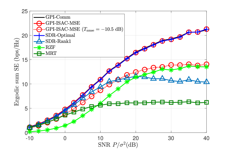
(a) Achieved SE

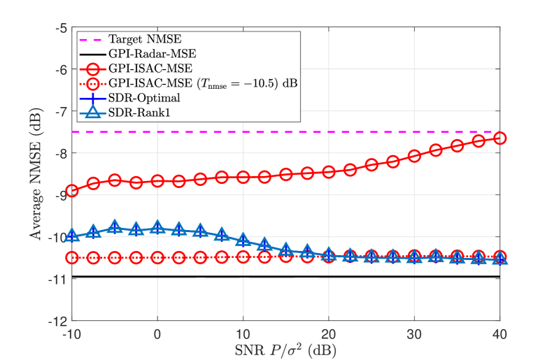
(b) Achieved NMSE

Figure 1: (a) The ergodic sum SE and (b) the average NMSE with respect to the SNR for $N=8$, $K=4$, $M=8$, and $T_{\rm nmse}=-7.5$ dB. Since SDR-based algorithms achieve a lower NMSE $\approx(-10.5\sim-10)$ dB, the GPI-ISAC result with $T_{\rm nmse}=-10.5$ dB is also included for comparison.

Now, we briefly introduce the existing approaches to solve optimization problems in ISAC systems for benchmark.

SDR-based Algorithm: Using the proposed optimization method in [26, 29], the following problem is solved, and beamforming performance is evaluated as a benchmark for GPI-ISAC with the MSE radar metric:

$$\mathop{\text{minimize}}_{{\bf{F}}}\;\; \frac{1}{L}\sum_{\ell=1}^{L}|Pd(\theta_{\ell})-B({\bf F};\theta_{\ell})|^{2}$$ (58)

subjectto $$\gamma_{k}\geq\Gamma_{k},\ \|{\bf{F}}\|_{\sf F}=1.$$ (59)

Since the radar metric (MSE) is placed in the objective function while the communication metrics (SINR) are placed in the constraints, the SDR-based algorithm can be viewed as a radar-oriented beamforming framework. For fair comparison, we set the quality of service (QoS) constraint $\Gamma_{k}$ as the SINRs achieved from GPI-ISAC (MSE). Since the SDR-based algorithm cannot handle the channel estimation error, it uses an estimated channel to compute $\gamma_{k}$. Due to the channel estimation error, the problem with such $\Gamma_{k}$ from GPI-ISAC (MSE) can be infeasible for some cases. Then we repeatedly reduce $\Gamma_{k},\forall k$ until the problem becomes feasible. We reduce $\Gamma_{k}$ by $10\%$ at each occurrence.

WMMSE-MM Algorithm: Using the proposed WMMSE-MM method in [31], the following problem is solved:

$$\mathop{\text{maximize}}_{{\bf{F}}}\;\; \sum_{k=1}^{K}R_{k}+\mu{\bf{a}}^{\sf H}(\theta^{*}){\bf{F}}{\bf{F}}^{\sf H}{\bf{a}}(\theta^{*})$$ (60)

subjectto $$\|{\bf{F}}\|_{\sf F}=1,$$ (61)

where $\theta^{*}$ is the desired radar beam direction. For comparison, we further adopt our binary-search based line search for finding $\mu$ that the derived $\bf F$ satisfies the same SCNR constraint as our problem in (15) with, and corresponding beamforming performance is evaluated as a benchmark for GPI-ISAC with the SCNR radar metric for a single-target case.

V-A MSE Radar Performance Metric

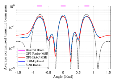
Figure 2: A normalized transmit beam pattern with the achieved NMSE $\approx-10.5$ dB for the GPI-ISAC and SDR-based algorithms at ${\rm SNR}=25$ dB. Corresponding sum SEs of GPI-ISAC-MSE and SDR-Rank1 are $13.4$ and $11.1$ ${\rm bps/Hz}$, respectively.

We first evaluate GPI-ISAC with the MSE constraint (GPI-ISAC-MSE) for multiple target angles located in $\{-\pi/4,0,\pi/4\}$ radians with the beam width of $\pi/36$ radian. To this end, the desired normalized beam pattern is shaped to be $d(\theta)=1$, centered around the target angles with the width of $\pi/6$, and $d(\theta)=0$ elsewhere. We consider $N=8$, $K=4$, and $M=8$. In simulations, GPI-Comm indicates the proposed GPI-ISAC algorithm without the radar constraint which reduces to the precoding algorithm in [43]. Accordingly, it is considered to provide a communication performance upper bound for GPI-ISAC with the MSE radar metric (GPI-ISAC-MSE). Similarly, GPI-Radar-MSE represents the proposed algorithm for the radar-only setup with radar beam MSE minimization, and hence, its radar MSE performance is regarded as a lower bound for GPI-ISAC-MSE.

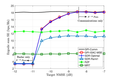
(a) Achieved SE

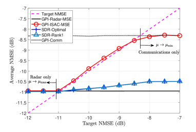
(b) Achieved NMSE

Figure 3: (a) The ergodic sum SE and (b) the average NMSE with respect to the target NMSE $T_{\rm nmse}$ for $N=8$, $K=4$, $M=8$, and ${\rm SNR}=40$ dB.

Fig. 1 shows (a) the ergodic sum SE and (b) the average NMSE with respect to the SNR for $T_{\rm nmse}=-7.5$ dB. It is observed that the SDR-based algorithm without rank-1 approximation (SDR-Optimal) achieves the same SE as GPI-ISAC-MSE with the lower MSE since it is optimal when ignoring the requirement for the rank-1 approximation. Note that this is indeed infeasible to use. To obtain the feasible beamforming vectors, rank-1 approximation is requisite. Fig. 1 reveals that GPI-ISAC-MSE provides the higher SE than the SDR-based algorithm after rank-1 approximation (SDR-Rank1) and RZF for $T_{\rm nmse}=-7.5$ dB while meeting the MSE constraint. In this regard, we observe that GPI-ISAC-MSE significantly outperforms SDR-Rank1 in terms of the SE while satisfying the MSE constraints. This is because SDR-Rank1 is a radar-oriented ISAC beamforming algorithm. For more comparison, the GPI-ISAC-MSE result with $T_{\rm nmse}=-10.5$ dB is also included in Fig. 1 since the SDR-based algorithms achieve NMSE $\approx-10.5$ dB as shown in Fig. 1(b). With the similar achieved NMSE, GPI-ISAC-MSE also offers better SE performance than SDR-Rank1 in most cases.

In Fig. 2, we further present the corresponding transmit beam patterns of the algorithms evaluated in Fig. 1 for $40$ dB SNR. The target beam angles are also marked. As expected, GPI-Radar-MSE shows the best beam pattern by achieving NMSE $\approx-11$ dB. GPI-ISAC-MSE ($T_{\rm nmse}=-10.5$ dB) and SDR-based algorithms provide almost the same beam pattern with each other as they achieve similar MSE performance while GPI-ISAC-MSE ($T_{\rm nmse}=-10.5$ dB) has the higher sum SE than SDR-Rank1 by $\sim\!\!3$ bps/Hz. This result implies that GPI-ISAC-MSE is more efficient and effective in providing th higher sum SE while accomplishing the required radar beamforming performance compared to SDR-Rank1.

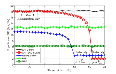
(a) Achieved SE

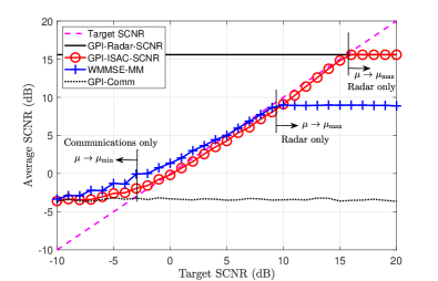
(b) Achieved SCNR

Figure 4: (a) The ergodic sum SE and (b) the average NMSE with respect to the SNR for $N=8$, $K=4$, $M=8$, and $25$ dB SNR.

Fig. 3 presents (a) the ergodic sum SE and (b) the average NMSE with respect to $T_{\rm nmse}$ for $N=8$, $K=4$, $M=8$, and $40$ dB SNR. It is shown in Fig. 3(a) that the sum SE increases as the target NMSE increases for GPI-ISAC-MSE and SDR-based algorithms. Beyond $-9.5$ dB, the SEs of GPI-ISAC-MSE and SDR-Optimal converge to that of GPI-Comm, which indicates that the NMSE target is too loose so that it is attainable without considering the constraint, i.e., $\mu=0$. When the target MSE is too stringent, the algorithms show a huge drop of the sum SE as they use the resource primarily to minimize the MSE. As shown in Fig. 3(b), the drop occurs when the target MSE becomes infeasible ($<-11$ dB). It is noticeable that the sum SE of GPI-ISAC-MSE is larger than that of SDR-Rank1 for the feasible target MSE. The sum SE gap between GPI-ISAC-MSE and SDR-Rank1 becomes larger with the higher target MSE because the SDR-based algorithms present unnecessarily lower MSE than the target as shown in Fig. 3(b). Unlike the SDR-based algorithms, GPI-ISAC-MSE provides the higher sum SE while closely meeting the target MSE. Fig. 3 reveals that the radar-oriented method is not preferable to use in terms of communications.

V-B SCNR Radar Performance Metric

Now, we evaluate GPI-ISAC with the SCNR constraint (GPI-ISAC-SCNR) for a single-target case in which the intensity of clutters is comparable to the reflected beam from the target. To this end, we set reflection coefficients of the target and clutters as $|\beta^{\rm tar}|=|\beta_{j}^{\rm cl}|=1$. The target angle is $\theta^{\rm tar}=\pi/6$ radian and clutter angles are $\theta^{\rm cl}_{j}\in\{-\pi/3,-\pi/8,\pi/3\}$. We consider $N=8$, $K=4$, $M=8$, and $25$ dB SNR.

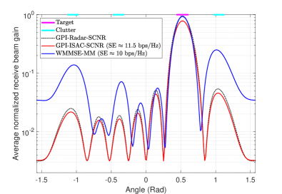
Figure 5: Normalized receive beam patterns of GPI-based algorithms and WMMSE-MM with the achieved sum SEs of $\sim\!11.5\ {\rm bps/Hz}$ and $\sim\!10\ {\rm bps/Hz}$ for GPI-ISAC-SCNR and WMMSE-MM, respectively.

We present the ergodic sum SE and the achieved SCNR performance for $25$ dB SNR in Fig. 4. As shown in Fig. 4, GPI-ISAC-SCNR achieves a much higher sum SE than WMMSE-MM and also the linear precoders for the feasible target SCNR range. When the target SCNR is low, the sum SEs of GPI-ISAC-SCNR and WMMSE-MM converge to different sum SEs. In particular, the sum SE of GPI-ISAC-SCNR converge to that of GPI-Comm as the target SCNR decreases. We notice that the convergence happens when the target SCNR becomes lower than the achieved SCNR of GPI-Comm, i.e., the target SCNR can be met with $\mu=0$. Contrary to this, both the algorithms reveals rapid drop of the sum SE beyond a certain target SCNR because they put most of the resources to maximize the SCNR, i.e., $\mu\to\mu_{\rm max}$. Such a significant drop of the sum SE is observed when the algorithms cannot satisfy the target SCNR ($>16$ dB) as shown in Fig. 4(b). With clutters, the feasible target SCNR range is wider for GPI-ISAC-SCNR than WMMSE-MM, which comes from the fact that WMMSE-MM does not take into account the clutters. Therefore, GPI-ISAC-SCNR is more desirable to use than WMMSE-MM in the presence of non-negligible clutters.

Fig. 5 illustrates a normalized receive beam gain over the angular grid: the normalized receive beam gain at each angle $\theta_{\ell}$ is computed as

$$\frac{1}{P}\mathbb{E}[|{\bf a}_{\rm r}^{\sf H}(\theta_{\ell}){\bf y}_{\rm R}|^{2}]={\bf a}_{\rm r}^{\sf H}\left({\bf G}{\bf F}{\bf F}^{\sf H}{\bf G}^{\sf H}+\frac{\sigma^{2}_{\rm R}}{P}{\bf I}_{N}\right){\bf a}_{\rm r},$$ (62)

where ${\bf G}={\bf G}_{\rm tar}+{\bf G}_{\rm cl}$. The achieved sum SEs are $\sim\!11.5\ {\rm bps/Hz}$ and $\sim\!10\ {\rm bps/Hz}$ for GPI-ISAC-SCNR and WMMSE-MM, respectively. Even with the higher sum SE, GPI-ISAC-SCNR shows the better receive beam pattern than WMMSE-MM, providing a comparable main lobe for the target angle with much lower side lobes; the achieved SCNR of GPI-ISAC-SCNR is approximately $15$ dB and that of WMMSE-MM is approximately $6$ dB. Thus, the proposed method outperforms WMMSE-MM in terms of both beam design accuracy and SE.

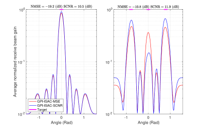
(a) No cluttering (single-target & multi-target)

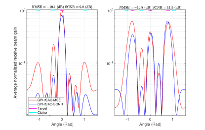
(b) Cluttering (single-target & multi-target)

Figure 6: Radar performance with regard to the number of targets and the intensity of cluttering at the achieved sum SE of $\sim\!\!10\ {\rm bps/Hz}$. The achieved NMSE of GPI-ISAC-MSE and SCNR of GPI-ISAC-SCNR are also presented.

V-C Comparison between MSE and SCNR metrics

Finally, we analyze the effect of using the MSE and SCNR as the radar performance metric for single-target, multi-target, no cluttering, and cluttering cases. In Fig. 6, the receive beam gains of GPI-ISAC-MSE and GPI-ISAC-SCNR are plotted for $N=8$, $K=6$, and $M=8$ at the achieved sum SE of $\sim\!\!10\ {\rm bps/Hz}$. When there is no or negligible clutter, GPI-ISAC-MSE and GPI-ISAC-SCNR provide almost similar beam patterns for the single-target case, whereas GPI-ISAC-MSE presents a better pattern with better-balanced main lobes and lower side lobes than GPI-ISAC-SCNR for the multi-target case as shown in Fig. 6(a). Such a result corresponds to the intuition that the MSE radar metric is adequate to design a multi-target beam without clutters.

In Fig. 6(b), the receive beam patterns are illustrated for the non-negligible cluttering environment. With the presence of a single target, GPI-ISAC-SCNR outperforms GPI-ISAC-MSE as its beam pattern shows similar main lobe with much lower side lobes than that of GPI-ISAC-MSE. This also aligns with the intuition that the SCNR metric is suitable for a single-target case considering non-negligible cluttering. A multi-target case, however, the beam patterns of both GPI-ISAC-MSE and GPI-ISAC-SCNR reveal trade-off: GPI-ISAC-MSE presents more even or stronger main lobes with higher side lobe whereas GPI-ISAC-SCNR shows lower side lobe with more uneven or weaker main lobes compared to each other. Accordingly, for such a harsh environment, either metric can be used depending on the types of radar systems. The analysis result from Fig. 6 is summarized in Table I.

VI Conclusion

In this paper, we proposed a joint beamforming framework for integrated sensing and communications systems with imperfect CSIT. Using a MSE or SCNR metric as a radar constraint, we formulated a communication-oriented problem to maximize a sum SE while satisfying the MSE or SCNR constraint. To solve the problem, we first reformulated the problem in terms of a vectorized joint beamformers, and then identified the KKT stationarity condition. Interpreting the condition as a functional eigenvalue problem, a GPI method was employed to derive the best local optimal solution. In simulations, the proposed GPI-ISAC algorithms demonstrated the superior communications and radar performance over the state-of-the-art ISAC methods with the imperfect CSIT. The compatibility of the different radar metrics was also analyzed, showing that the MSE metric is effective in multi-target and no-cluttering environments and the SCNR metric is useful in single-target and intense-cluttering environments. In addition, when the beam requirement is easy or stringent to fulfil, both the metrics can be used. Therefore, it is concluded that the proposed ISAC beamforming framework is comprehensive and robust, and it can readily be applied for various ISAC environments, providing high communication and radar efficiency.

TABLE I: A Preferred Radar Performance Metric for Different Cases

2 Case	Low Clutter Intensity	High Clutter Intensity
Few Targets	MSE, SCNR	SCNR
Many Targets	MSE	MSE, SCNR
2

Appendix A Proof of Lemma 1

We first normalize the MSE constraint with respect to the transmit power $P$ to make the scale of the constraint comparable to the objective function as

$$\frac{1}{LP^{2}}\sum_{\ell=1}^{L}|\bar{\bf{f}}^{\sf H}{\bf{D}}(\theta_{\ell})\bar{\bf{f}}-\bar{\bf{f}}^{\sf H}{\bf{A}}(\theta_{\ell})\bar{\bf{f}}|^{2}\leq\frac{T_{\rm mse}}{P^{2}}.$$ (63)

The Lagrangian function of (30) with the MSE in (63) is

$$L(\bar{\bf{f}};\mu) =\log_{2}\prod_{k=1}^{K}\left(\frac{\bar{\bf{f}}^{\sf H}{\bf{B}}_{k}\bar{\bf{f}}}{\bar{\bf{f}}^{\sf H}{\bf{C}}_{k}\bar{\bf{f}}}\right)+$$

$$\quad\mu\left(\frac{T_{\rm mse}}{P^{2}}-\frac{1}{LP^{2}}\sum_{\ell=1}^{L}|\bar{\bf{f}}^{\sf H}{\bf{D}}(\theta_{\ell})\bar{\bf{f}}-\bar{\bf{f}}^{\sf H}{\bf{A}}(\theta_{\ell})\bar{\bf{f}}|^{2}\right)$$ (64)

$$=\log_{2}\lambda(\bar{\bf{f}}),$$ (65)

where $\mu$ is the Lagrangian multiplier and $\lambda(\bar{\bf{f}})$ is defined in (36). The stationarity condition requires

$$\frac{\partial L(\bar{\bf{f}},\mu)}{\partial\bar{\bf{f}}}=\frac{\partial L(\bar{\bf{f}},\mu)}{\partial\lambda(\bar{\bf{f}})}\frac{\partial\lambda(\bar{\bf{f}})}{\partial\bar{\bf{f}}}=\frac{1}{\lambda(\bar{\bf{f}})\log 2}\frac{\partial\lambda(\bar{\bf{f}})}{\partial\bar{\bf{f}}}=0.$$ (66)

Accordingly, we find the condition for $\frac{\partial\lambda(\bar{\bf{f}})}{\partial\bar{\bf{f}}}=0$ which is equivalent to $\eqref{eq:derivative}$. With direct matrix calculus and simplification, we have

$$\frac{\partial\lambda(\bar{\bf{f}})}{\partial\bar{\bf{f}}}= 2\lambda(\bar{\bf{f}})\left[\sum_{k=1}^{K}\Bigg{(}\frac{{\bf{B}}_{k}\bar{\bf{f}}}{\bar{\bf{f}}^{\sf H}{\bf{B}}_{k}\bar{\bf{f}}}-\frac{{\bf{C}}_{k}\bar{\bf{f}}}{\bar{\bf{f}}^{\sf H}{\bf{C}}_{k}\bar{\bf{f}}}\Bigg{)}\right.$$

$$\left.+\frac{2\mu\log 2}{LP^{2}}\sum_{\ell=1}^{L}\Bigg{(}\left(\bar{\bf{f}}^{\sf H}{\bf{A}}(\theta_{\ell})\bar{\bf{f}}-\bar{\bf{f}}^{\sf H}{\bf{D}}(\theta_{\ell})\bar{\bf{f}}\right){\bf{D}}(\theta_{\ell})\bar{\bf{f}}\right.$$

$$\left.-\left(\bar{\bf{f}}^{\sf H}{\bf{A}}(\theta_{\ell})\bar{\bf{f}}-\bar{\bf{f}}^{\sf H}{\bf{D}}(\theta_{\ell})\bar{\bf{f}}\right){\bf{A}}(\theta_{\ell})\bar{\bf{f}}\Bigg{)}\right]=0.$$ (67)

Rearranging the condition in (67) carefully, we have

$$\lambda_{\sf num}(\bar{\bf f})\left[\sum_{k=1}^{K}\frac{{\bf{B}}_{k}}{\bar{\bf{f}}^{\sf H}{\bf{B}}_{k}\bar{\bf{f}}}+\right.$$

$$\left.\frac{2\mu\log 2}{LP^{2}}\sum_{\ell=1}^{L}\left\{(\bar{\bf{f}}^{\sf H}{\bf{D}}(\theta_{\ell})\bar{\bf{f}}){\bf{A}}(\theta_{\ell})+(\bar{\bf{f}}^{\sf H}{\bf{A}}(\theta_{\ell})\bar{\bf{f}}){\bf{D}}(\theta_{\ell})\right\}\right]\bar{\bf{f}}$$

$$=\lambda_{\sf den}(\bar{\bf f})\left[\sum_{k=1}^{K}\frac{{\bf{C}}_{k}}{\bar{\bf{f}}^{\sf H}{\bf{C}}_{k}\bar{\bf{f}}}+\right.$$

$$\left.\frac{2\mu\log 2}{LP^{2}}\sum_{\ell=1}^{L}\left\{(\bar{\bf{f}}^{\sf H}{\bf{D}}(\theta_{\ell})\bar{\bf{f}})\alpha{\bf{D}}(\theta_{\ell})+(\bar{\bf{f}}^{\sf H}{\bf{A}}(\theta_{\ell})\bar{\bf{f}}){\bf{A}}(\theta_{\ell})\right\}\right]\lambda({\bar{\bf f}})\bar{\bf{f}}.$$

This completes the proof. $\blacksquare$

Appendix B Proof of Lemma 2

We first convert the SCNR constraint into a log-scale to make the scale of the constraint comparable to the sum SE as

$$\log_{2}\left(\frac{\bar{\bf f}^{\sf H}{\bar{\bf G}}_{\rm tar}\bar{\bf f}}{\bar{\bf f}^{\sf H}{\bar{\bf G}}_{\rm cl}\bar{\bf f}}\right)\geq\log_{2}T_{\rm scnr}.$$ (68)

The Lagrangian function of (42) with (68) is

$$\tilde{L}(\bar{\bf{f}};\mu) =\log_{2}\prod_{k=1}^{K}\left(\frac{\bar{\bf{f}}^{\sf H}{\bf{B}}_{k}\bar{\bf{f}}}{\bar{\bf{f}}^{\sf H}{\bf{C}}_{k}\bar{\bf{f}}}\right)+\mu\left(\log_{2}\left(\frac{\bar{\bf f}^{\sf H}{\bar{\bf G}}_{\rm tar}\bar{\bf f}}{\bar{\bf f}^{\sf H}{\bar{\bf G}}_{\rm cl}\bar{\bf f}}\right)-\log_{2}T_{\rm scnr}\right)$$

$$=\log_{2}\eta(\bar{\bf{f}}),$$ (69)

where $\mu$ is the Lagrangian multiplier and $\eta(\bar{\bf{f}})$ is defined in (49). The stationarity condition requires

$$\frac{\partial\tilde{L}(\bar{\bf{f}},\mu)}{\partial\bar{\bf{f}}}=\frac{\partial\tilde{L}(\bar{\bf{f}},\mu)}{\partial\eta(\bar{\bf{f}})}\frac{\partial\eta(\bar{\bf{f}})}{\partial\bar{\bf{f}}}=\frac{1}{\eta(\bar{\bf{f}})\log 2}\frac{\partial\eta(\bar{\bf{f}})}{\partial\bar{\bf{f}}}.$$ (70)

Accordingly, we find the condition for $\frac{\partial\eta(\bar{\bf{f}})}{\partial\bar{\bf{f}}}=0$.

$$\frac{\partial\eta(\bar{\bf{f}})}{\partial\bar{\bf{f}}} \!=\!2\eta(\bar{\bf{f}})\left[\sum_{k=1}^{K}\Bigg{(}\frac{{\bf{B}}_{k}\bar{\bf{f}}}{\bar{\bf{f}}^{\sf H}{\bf{B}}_{k}\bar{\bf{f}}}\!-\!\frac{{\bf{C}}_{k}\bar{\bf{f}}}{\bar{\bf{f}}^{\sf H}{\bf{C}}_{k}\bar{\bf{f}}}\Bigg{)}\!+\!\mu\Bigg{(}\frac{{\bar{\bf G}}_{\rm tar}\bar{\bf f}}{\bar{\bf f}^{\sf H}{\bar{\bf G}}_{\rm tar}\bar{\bf{f}}}\!-\!\frac{{\bar{\bf G}}_{\rm cl}\bar{\bf f}}{\bar{\bf f}^{\sf H}{\bar{\bf G}}_{\rm cl}\bar{\bf{f}}}\Bigg{)}\right]$$

$$=0.$$ (71)

Rearranging the condition in (71) carefully, we have

$$\eta_{\sf num}(\bar{\bf f})\left(\sum_{k=1}^{K}\frac{{\bf{B}}_{k}}{\bar{\bf{f}}^{\sf H}{\bf{B}}_{k}\bar{\bf{f}}}+\mu\frac{{\bar{\bf G}}_{\rm tar}}{\bar{\bf f}^{\sf H}{\bar{\bf G}}_{\rm tar}\bar{\bf{f}}}\right)\bar{\bf{f}}$$ (72)

$$=\eta_{\sf den}(\bar{\bf f})\left(\sum_{k=1}^{K}\frac{{\bf{C}}_{k}}{\bar{\bf{f}}^{\sf H}{\bf{C}}_{k}\bar{\bf{f}}}+\mu\frac{{\bar{\bf G}}_{\rm cl}}{\bar{\bf f}^{\sf H}{\bar{\bf G}}_{\rm cl}\bar{\bf{f}}}\right)\eta({\bar{\bf f}})\bar{\bf{f}}.$$ (73)

This completes the proof. $\blacksquare$

References

- [1] W. Saad, M. Bennis, and M. Chen, “A vision of 6G wireless systems: Applications, trends, technologies, and open research problems,” IEEE Network, vol. 34, no. 3, pp. 134–142, 2019.
- [2] F. Liu, Y. Cui, C. Masouros, J. Xu, T. X. Han, Y. C. Eldar, and S. Buzzi, “Integrated sensing and communications: Toward dual-functional wireless networks for 6g and beyond,” IEEE J. on Sel. Areas in Commun., vol. 40, no. 6, pp. 1728–1767, 2022.
- [3] M. L. Rahman, J. A. Zhang, X. Huang, Y. J. Guo, and R. W. Heath, “Framework for a perceptive mobile network using joint communication and radar sensing,” IEEE Trans. on Aerospace and Electronic Systems, vol. 56, no. 3, pp. 1926–1941, 2019.
- [4] F. Liu, C. Masouros, A. P. Petropulu, H. Griffiths, and L. Hanzo, “Joint radar and communication design: Applications, state-of-the-art, and the road ahead,” IEEE Trans. on Commun., vol. 68, no. 6, pp. 3834–3862, 2020.
- [5] R. Saruthirathanaworakun, J. M. Peha, and L. M. Correia, “Opportunistic sharing between rotating radar and cellular,” IEEE J. Sel. Areas Commun., vol. 30, no. 10, pp. 1900–1910, 2012.
- [6] S.-S. Raymond, A. Abubakari, and H.-S. Jo, “Coexistence of power-controlled cellular networks with rotating radar,” IEEE J. Sel. Areas Commun., vol. 34, no. 10, pp. 2605–2616, 2016.
- [7] S. Sodagari, A. Khawar, T. C. Clancy, and R. McGwier, “A projection based approach for radar and telecommunication systems coexistence,” in IEEE Global Commun. Conf. (GLOBECOM), 2012, pp. 5010–5014.
- [8] J. Qian, M. Lops, L. Zheng, X. Wang, and Z. He, “Joint system design for coexistence of MIMO radar and MIMO communication,” IEEE Trans. Signal Process., vol. 66, no. 13, pp. 3504–3519, 2018.
- [9] F. Liu, C. Masouros, A. Li, and T. Ratnarajah, “Robust MIMO beamforming for cellular and radar coexistence,” IEEE Wireless Commun. Lett., vol. 6, no. 3, pp. 374–377, 2017.
- [10] B. Paul, A. R. Chiriyath, and D. W. Bliss, “Survey of RF communications and sensing convergence research,” IEEE Access, vol. 5, pp. 252–270, 2017.
- [11] L. Zheng, M. Lops, Y. C. Eldar, and X. Wang, “Radar and communication coexistence: An overview: A review of recent methods,” IEEE Signal Process. Mag., vol. 36, no. 5, pp. 85–99, 2019.
- [12] P. Kumari, J. Choi, N. González-Prelcic, and R. W. Heath, “IEEE 802.11ad-based radar: An approach to joint vehicular communication-radar system,” IEEE Trans. Veh. Technol., vol. 67, no. 4, pp. 3012–3027, 2018.
- [13] D. Ma, N. Shlezinger, T. Huang, Y. Liu, and Y. C. Eldar, “Joint radar-communication strategies for autonomous vehicles: Combining two key automotive technologies,” IEEE Signal Process. Mag., vol. 37, no. 4, pp. 85–97, 2020.
- [14] F. Liu, Y. Cui, C. Masouros, J. Xu, T. X. Han, Y. C. Eldar, and S. Buzzi, “Integrated sensing and communications: Towards dual-functional wireless networks for 6g and beyond,” IEEE J. Sel. Areas Commun., pp. 1–1, 2022.
- [15] C. Sturm and W. Wiesbeck, “Waveform design and signal processing aspects for fusion of wireless communications and radar sensing,” Proceedings of the IEEE, vol. 99, no. 7, pp. 1236–1259, 2011.
- [16] A. R. Chiriyath, B. Paul, G. M. Jacyna, and D. W. Bliss, “Inner bounds on performance of radar and communications co-existence,” IEEE Trans. Signal Process., vol. 64, no. 2, pp. 464–474, 2016.
- [17] G. Choi and N. Lee, “Information-Theoretical Approach to Integrated Pulse-Doppler Radar and Communication Systems,” arXiv preprint arXiv:2302.05046, 2023.
- [18] Y. Liu, G. Liao, J. Xu, Z. Yang, and Y. Zhang, “Adaptive OFDM integrated radar and communications waveform design based on information theory,” IEEE Commun. Lett., vol. 21, no. 10, pp. 2174–2177, 2017.
- [19] J. Moghaddasi and K. Wu, “Multifunctional transceiver for future radar sensing and radio communicating data-fusion platform,” vol. 4, pp. 818–838, 2016.
- [20] M. F. Keskin, V. Koivunen, and H. Wymeersch, “Limited feedforward waveform design for OFDM dual-functional radar-communications,” IEEE Trans. Signal Process., vol. 69, pp. 2955–2970, 2021.
- [21] A. Hassanien, M. G. Amin, Y. D. Zhang, and F. Ahmad, “Dual-function radar-communications: Information embedding using sidelobe control and waveform diversity,” IEEE Trans. Signal Process., vol. 64, no. 8, pp. 2168–2181, 2016.
- [22] D. Ma, N. Shlezinger, T. Huang, Y. Liu, and Y. C. Eldar, “FRaC: FMCW-based joint radar-communications system via index modulation,” IEEE J. Sel. Topics Signal Process., vol. 15, no. 6, pp. 1348–1364, 2021.
- [23] T. Huang, N. Shlezinger, X. Xu, Y. Liu, and Y. C. Eldar, “MAJoRCom: A dual-function radar communication system using index modulation,” IEEE Trans. Signal Process., vol. 68, pp. 3423–3438, 2020.
- [24] D. Ma, N. Shlezinger, T. Huang, Y. Shavit, M. Namer, Y. Liu, and Y. C. Eldar, “Spatial modulation for joint radar-communications systems: Design, analysis, and hardware prototype,” IEEE Trans. Veh. Technol., vol. 70, no. 3, pp. 2283–2298, 2021.
- [25] W. Baxter, E. Aboutanios, and A. Hassanien, “Joint radar and communications for frequency-hopped MIMO systems,” IEEE Trans. Signal Process., vol. 70, pp. 729–742, 2022.
- [26] F. Liu, C. Masouros, A. Li, H. Sun, and L. Hanzo, “MU-MIMO communications with MIMO radar: From co-existence to joint transmission,” IEEE Trans. Wireless Commun., vol. 17, no. 4, pp. 2755–2770, 2018.
- [27] F. Liu, L. Zhou, C. Masouros, A. Li, W. Luo, and A. Petropulu, “Toward dual-functional radar-communication systems: Optimal waveform design,” IEEE Trans. Signal Process., vol. 66, no. 16, pp. 4264–4279, 2018.
- [28] H. Hua, J. Xu, and T. X. Han, “Optimal transmit beamforming for integrated sensing and communication,” IEEE Trans. on Veh. Technol., vol. 72, no. 8, pp. 10 588–10 603, 2023.
- [29] X. Liu, T. Huang, N. Shlezinger, Y. Liu, J. Zhou, and Y. C. Eldar, “Joint transmit beamforming for multiuser MIMO communications and MIMO radar,” IEEE Trans. Signal Process., vol. 68, pp. 3929–3944, 2020.
- [30] L. Chen, F. Liu, W. Wang, and C. Masouros, “Joint radar-communication transmission: A generalized pareto optimization framework,” IEEE Trans. Signal Process., vol. 69, pp. 2752–2765, 2021.
- [31] C. Xu, B. Clerckx, and J. Zhang, “Multi-antenna joint radar and communications: Precoder optimization and weighted sum-rate vs probing power tradeoff,” IEEE Access, vol. 8, pp. 173 974–173 982, 2020.
- [32] X. Liu, T. Huang, and Y. Liu, “Transmit design for joint MIMO radar and multiuser communications with transmit covariance constraint,” IEEE J. Sel. Areas Commun., pp. 1–1, 2022.
- [33] N. Su, F. Liu, and C. Masouros, “Secure Radar-Communication Systems With Malicious Targets: Integrating Radar, Communications and Jamming Functionalities,” IEEE Trans. Wireless Commun., vol. 20, no. 1, pp. 83–95, 2021.
- [34] Z. Ren, L. Qiu, J. Xu, and D. W. K. Ng, “Robust transmit beamforming for secure integrated sensing and communication,” IEEE Trans. on Commun., 2023.
- [35] C. Xu, B. Clerckx, S. Chen, Y. Mao, and J. Zhang, “Rate-splitting multiple access for multi-antenna joint radar and communications,” IEEE J. Sel. Topics Signal Process., pp. 1–1, 2021.
- [36] X. Mu, Y. Liu, L. Guo, J. Lin, and L. Hanzo, “NOMA-aided joint radar and multicast-unicast communication systems,” IEEE J. Sel. Areas Commun., pp. 1–1, 2022.
- [37] C. B. Barneto, T. Riihonen, M. Turunen, L. Anttila, M. Fleischer, K. Stadius, J. Ryynänen, and M. Valkama, “Full-duplex OFDM radar with LTE and 5G NR waveforms: Challenges, solutions, and measurements,” IEEE Trans. on Microwave Theory and Techniques, vol. 67, no. 10, pp. 4042–4054, 2019.
- [38] J. Kim, H. Lee, H. Do, J. Choi, J. Park, W. Shin, Y. C. Eldar, and N. Lee, “On the Learning of Digital Self-Interference Cancellation in Full-Duplex Radios,” arXiv preprint arXiv:2308.05966, 2023.
- [39] G. Cui, H. Li, and M. Rangaswamy, “MIMO radar waveform design with constant modulus and similarity constraints,” IEEE Trans. on Signal Process., vol. 62, no. 2, pp. 343–353, 2013.
- [40] H. Joudeh and B. Clerckx, “Sum-rate maximization for linearly precoded downlink multiuser MISO systems with partial CSIT: A rate-splitting approach,” IEEE Trans. Commun., vol. 64, no. 11, pp. 4847–4861, 2016.
- [41] J. Park, J. Choi, N. Lee, W. Shin, and H. V. Poor, “Rate-splitting multiple access for downlink MIMO: A generalized power iteration approach,” IEEE Trans. on Wireless Commun., vol. 22, no. 3, pp. 1588–1603, 2022.
- [42] Y. Cai, L.-H. Zhang, Z. Bai, and R.-C. Li, “On an eigenvector-dependent nonlinear eigenvalue problem,” SIAM Journal on Matrix Analysis and Applications, vol. 39, no. 3, pp. 1360–1382, 2018.
- [43] J. Choi, N. Lee, S. Hong, and G. Caire, “Joint user selection, power allocation, and precoding design with imperfect CSIT for multi-cell MU-MIMO downlink systems,” IEEE Trans. Wireless Commun., vol. 19, no. 1, pp. 162–176, 2020.
- [44] A. Adhikary, J. Nam, J. Ahn, and G. Caire, “Joint spatial division and multiplexing - The large-scale array regime,” IEEE Trans. Inf. Theory, vol. 59, no. 10, pp. 6441–6463, Oct. 2013.
- [45] J. Park, N. Lee, J. G. Andrews, and R. W. Heath, “On the optimal feedback rate in interference-limited multi-antenna cellular systems,” IEEE Trans. on Wireless Commun., vol. 15, no. 8, pp. 5748–5762, 2016.