ResQuNNs:Towards Enabling Deep Learning in
Quantum Convolution Neural Networks

Abstract.

In this paper, we present a novel framework for enhancing the performance of Quanvolutional Neural Networks (QuNNs) by introducing trainable quanvolutional layers and addressing the critical challenges associated with them. Traditional quanvolutional layers, although beneficial for feature extraction, have largely been static, offering limited adaptability. Unlike state-of-the-art, our research overcomes this limitation by enabling training within these layers, significantly increasing the flexibility and potential of QuNNs. However, the introduction of multiple trainable quanvolutional layers induces complexities in gradient-based optimization, primarily due to the difficulty in accessing gradients across these layers. To resolve this, we propose a novel architecture, Residual Quanvolutional Neural Networks (ResQuNNs), leveraging the concept of residual learning, which facilitates the flow of gradients by adding skip connections between layers. By inserting residual blocks between quanvolutional layers, we ensure enhanced gradient access throughout the network, leading to improved training performance. Moreover, we provide empirical evidence on the strategic placement of these residual blocks within QuNNs. Through extensive experimentation, we identify an efficient configuration of residual blocks, which enables gradients across all the layers in the network that eventually results in efficient training. Our findings suggest that the precise location of residual blocks plays a crucial role in maximizing the performance gains in QuNNs. Our results mark a substantial step forward in the evolution of quantum deep learning, offering new avenues for both theoretical development and practical quantum computing applications.

1. Introduction

Quantum Convolutional Neural Networks (QCNNs) represent an innovative fusion of quantum computing principles with traditional convolutional neural network (CNN) architectures (Wei et al., 2022; Zaman et al., 2023). These hybrid classical-quantum models utilize parameterized quantum circuits (PQCs) a.k.a ansatz, composed of parameterized rotation gates such as Rx, Ry, or Rz, functioning analogously to convolutional and pooling operations in classical CNNs (Cong et al., 2019; Rajesh et al., 2021). The optimization of these models, however, is performed on classical computers (Hur et al., 2022; Shen et al., 2023).

A notable advantage of QCNNs lies in their ability to harness the vast Hilbert space offered by quantum mechanics, which surpasses the capabilities of classical CNNs (Schuld and Killoran, 2019). This feature allows QCNNs to capture spatial relationships in image data more effectively. Furthermore, the potential future inclusion of higher-level quantum systems, such as qutrits or ququads (Sebastian et al., 2023; Hu et al., 2023), promises even more sophisticated image comprehension capabilities.

There are two primary variants of QCNNs, each leveraging quantum mechanics principles like superposition, entanglement, and interference. The first type, Quantum-Inspired CNNs, proposed in (Cong et al., 2019), mirrors the structure of classical CNNs but replaces convolutional and pooling layers with deeper PQCs. This design demands higher qubit coherence to fully exploit quantum parallelism and entanglement, posing a challenge for current quantum hardware. Nevertheless, a significant research has been dedicated to explore this very architectural framework for various applications (Hur et al., 2022; Kim et al., 2023). The second type, Quanvolutional Neural Networks (QuNNs), first introduced in (Henderson et al., 2020), and visually depicted in Figure 1, focuses on quantum-enhanced convolutional layers. These networks encode classical image pixels into quantum states, apply unitary transformations via PQCs, and then measure the qubits to create output image channels, which are subsequently processed by classical fully connected layers. This approach offers a more feasible implementation with current quantum technology.

QuNNs have widely been used in the literature for various applications such as 2D and 3D radiological image classification (Matic et al., 2022), analysing the high energy physics data (Chen et al., 2022), for object detection and classification (Meedinti et al., 2023; Baek et al., 2022). In light of the capabilities and constraints of present-day quantum hardware, this paper also delves into QuNNs. Our primary focus is on identifying the challenges faced in training QuNNs and proposing effective solutions to address these issues.

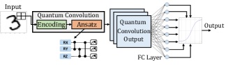
Figure 1. Quanvolutional Neural Network Architecture.

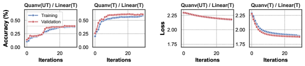
Figure 2. Motivational analysis showing the impact of making quanvolutional layers trainable. UT = Untrainable, T = Trainable.

1.1. Motivational Analysis

QuNNs, as shown in Figure 1 performs the convolution on the input image within the grey-shaded region. This process involves sequentially encoding a small region of the input image into quantum space, while moving a kernel across the image, indicated by the green-shaded area of Figure 1. A unitary transformation is then applied to a small square region of the input via the ansatz, as depicted in the brown region of Figure 1. The output of this quanvolution (a quantum circuit-based convolution) is then processed by a classical neural network to produce the final network output. While this architecture is standard in many state-of-the-art works, a key challenge is the non-trainable nature of the quanvolution operation, primarily used for input preprocessing. Consequently, the learning process is primarily driven by the subsequent classical network. For QuNNs to be fully scalable, ensuring the trainability of underlying quanvolutional layers is crucial.

In Figure 2, we examined the impact of trainable versus untrainable quanvolutional layers in QuNNs. We trained these layers on 1000 randomly chosen MNIST dataset images over 30 iterations, using an 80%-20% training-validation split. The Adam optimizer with a $0.01$ learning rate was employed. We utilized a $2\times 2$ kernel resulting in 4-qubit quanvolutional layers, with each layer comprising of 4 parameterized $R_{y}$ gates and 4 $CNOT$ entanglement gates. The total layer depth was set to 5.

To scrutinize the impact of a (trainable/untrainable) quanvolutional layer, we compared models with trainable quanvolutional layers (allowing weight updates during backpropagation) against those with untrainable layers (frozen weights, no updates). Results showed suboptimal performance when quanvolutional layers were untrainable and only the final fully connected (FC) layer was trained. Conversely, allowing weight updates in the quanvolutional layers significantly improved learning, enhancing model accuracy by approximately 36%. This empirical evidence robustly substantiates the hypothesis that facilitating the trainability of quanvolutional layers significantly augments the model’s overall learning efficacy, as we notice an improvement in performance by approximately 36% in terms of achieved accuracy.

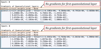
Figure 3. Gradients Propagation for Two (upper pannel) and Three Quanvolutional Layers (lower panel)

While a single trainable quanvolutional layer enhances QuNNs’ training efficacy, as depicted in Figure 1.1, scalability requires multiple trainable layers. Also, the rationale for using multiple layers is to avoid the problem of vanishing gradients a.k.a Barren Plateaus (BP), common in single, more expressive PQCs with a higher qubit count and sufficient depth(McClean et al., 2018; M.Kashif and Al-Kuwari, 2023; Kashif et al., 2023). Multiple layers, with progressively smaller quantum circuits, can potentially mitiagte the BPs(Kashif and Al-kuwari, 2024). However, challenges emerge when multiple quanvolutional layers are trained concurrently, as gradients become exclusively accessible only in the last layer, limiting the optimization process only to this layer. Figure 3 demonstrates this by showing gradients for two and three cascaded trainable quanvolutional layers.

We observe that the gradients of only the final layer are accessible, while those of the preceding layers are effectively None. This means that in multi-layer QuNNs, only the final layer benefits from backpropagation, leaving earlier layers uninvolved in optimization. This presents a significant challenge in effectively training multi-layered QuNNs. This presents a substantial obstacle to concurrent training of multiple quanvolutional layers, thereby necessitating innovative approaches to address this challenge in the pursuit of scalable and effective QuNN architectures.

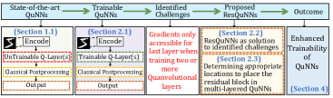
Figure 4. Overview of our contributions

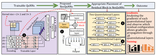
Figure 5. Detailed Methodology. A comprehensive overview of steps involved in the analysis of trainable QuNNs and proposed ResQuNNs. QCL = Quanvolutional Layer

1.2. Novel Contributions

Our primary contributions encompass the introduction of trainable quanvolutional layers, recognition of challenges with multiple quanvolutional layers, the development of Residual Quantum Convolutional Neural Networks (ResQuNNs) to address these challenges, and empirical findings on the strategic placement of residual blocks to enhance training performance. An overview of our contributions is shown in Figure 4.

• Trainable Quanvolutional Layers: We introduce the concept of making quanvolutional layers trainable, addressing the challenge of enhancing their adaptability within QuNNs and enhancing their training performance.

• Challenges with Multiple Quanvolutional Layers: The paper identifies a key challenge in optimizing multiple quanvolutional layers, highlighting the complexities associated with accessing gradients across these layers making then unsuitable for gradient-based optimization techniques.

• Residual Quantum Convolutional Neural Networks (ResQuNN): To overcome the gradient accessibility issue, this paper introduces Residual Quantum Convolutional Neural Networks (ResQuNN), drawing inspiration from classical residual neural networks.

• Residual Blocks for Gradient Accessibility: In ResQuNNs, residual blocks between quanvolutional layers are incorporated to facilitate comprehensive gradient access, thereby improving training performance. These residual blocks combine the output of existing quanvolutional layers with their own or previous layer’s input before forwarding it to the subsequent quanvolutional layer.

• Strategic Placement of Residual Blocks: We conducted extensive experiments to determine optimal locations for inserting residual blocks within networks comprising of multiple quanvolutional layers.

2. Proposed Methodology

The detailed overview of methodology is presented in Figure 5. Below we discuss different steps of our methodology in detail.

2.1. Trainable Quanvolutional Layers in QuNNs.

The first key aspect of our methodology involves the concept of making quanvolutional layers trainable. The majority of works in the literature utilizes these layers for efficient feature extraction and pass the output to classical layers, however, the quanvolution operation itself is not trainable. We recognize the need to enhance the adaptability of these layers within QuNNs and introduce trainable quanvolutional layers to harness their full potential. We do this by making the quanvolution layer to a pytorch layer which is later used a layer during the model construction. The trainable QuNN utilized in this study is depicted in Figure 5, marked as label , and operates through the following steps.

1. A small region of input image is sequentially encoded using a kernel of size $2\times 2$ and $3\times 3$ into quantum states, specifically into the rotation angles of $RY$ gates, which can be described by the following rotation matrix:

   $$R_{\text{Y}}(\theta)=\begin{bmatrix}\cos(\theta/2)&-\sin(\theta/2)\\ \sin(\theta/2)&\cos(\theta/2)\\ \end{bmatrix}$$

2. The encoded data then undergoes a unitary transformation, which is achieved through a PQC. We call this PQC, quanvolutional layer throughout this paper. In case of two quanvolutional layers, the first quanvolutional layer has a depth of $5$, while that of second has a depth of 1. This configuration is strategically chosen to distinctly evaluate the impact on performance when gradients from both layers are accessible in ResQuNNs, in contrast to situations where only gradients from the second layer are accessible.

3. The quanvolutional layers are finally measured, yielding a list of classical expectation values. Similar to a classical convolution layer, each expectation value corresponds to a separate channel in a single output pixel.

4. The outputs are then passed to fully connected classical layer to meaningfully postprocess the results of quanvolutional layers.

2.2. Residual Quanvolutional Neural Networks (ResQuNNs).

To overcome the gradient accessibility issue encountered in mulyi-layered QuNNs, as discussed in Section 1.1, we introduce ResQuNNs. Drawing inspiration from classical residual neural networks, ResQuNNs incorporate residual blocks between quanvolutional layers. The residual blocks combine the output of existing quanvolutional layers with their own or the previous layer’s input before forwarding it to the subsequent quanvolutional layer, as shown in label in Figure 5, and play a pivotal role in facilitating comprehensive gradient access and, in turn, improving the overall training performance of QuNNs.

2.3. Strategic Placement of Residual Blocks.

Within the ResQuNN architecture, residual blocks needs to be strategically placed between quanvolutional layers. In our empirical investigation, we conduct extensive experimentation to determine the appropriate locations for inserting residual blocks within ResQuNNs comprising two quanvolutional layers, as shown in Figure 5, labeled . This analysis helps us uncover the most effective residual configurations for ResQuNNs, enabling us to fine-tune the proposed ResQuNN architecture for enhanced training performance. We selected only the most successful configurations from this phase for further analysis in three-layer quanvolutional setups, as marked by label in Figure 5.

We trained ResQuNNs across all residual configurations for a multiclass classification problem to understand the impact of gradient accessibility across all the layers of the network on QuNNs’ overall performance. The training details and outcomes are discussed in the following section.

3. Experimental Setup

We trained the proposed ResQuNNs on a selected subset of the MNIST dataset, comprising 200 images randomly selected from each class of the training set, amounting to a total of 2000 images. This subset was subsequently split into training and validation sets, with an 80% to 20% distribution, respectively. An overview of the experimental toolflow utilized in this paper is depicted in Figure 6.

The objective function chosen for training is cross entropy loss, which can be described (for C classes) by the following equation:

$$H(p,q)=-\sum_{c=1}^{C}p(c)\log(q(c))$$

where H(p,q) is the cross entropy loss., p(c) represents the true probability distribution for class c, q(c) denotes the predicted probability distribution for class. All experiments are executed utilizing Pennylane, a Python library tailored for differentiable programming on quantum computing platforms (Bergholm et al., 2018).

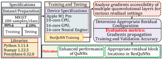
Figure 6. Overview of Our Experimental Tool-flow

4. Results

In this section, we present the outcomes resulting from our experimental investigations, meticulously organized and subjected to thorough analysis, with the aim of deriving meaningful conclusions. Our experimental scope encompassed the exploration of both two and three trainable quanvolutional layers.

4.1. Two Quanvolutional Layers

4.1.1. $\textbf{2}\times\textbf{2}$ Kernel

The kernel size of $2\times 2$ results in 4-qubit quanvolutional layers. Our experimental framework involved extensive testing of all residual configurations as outlined in label of Figure 5, employing a kernel size of $2\times 2$. For each residual configuration, we investigated the gradient propagation through the quanvolutional layers. We then trained the ResQuNNs for all these configurations to assess the impact of gradient accessibility throughout the network’s layers.

Analysis of Gradients Accessibility

In the case of No Residual setting, as previously shown in Figure 3, we have already established the fact that the gradients are exclusively accessible for the second quanvolutional layer. Subsequently, we proceeded to investigate the gradient propagation through the quanvolutional layers for all other residual settings, as illustrated in Figure 7.

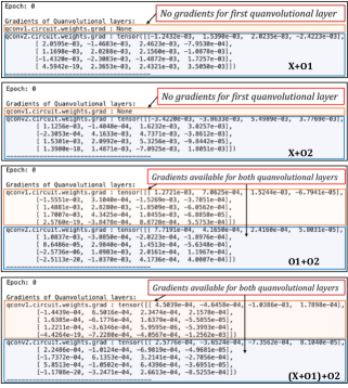
Figure 7. Gradients Propagation Through the Network for Two Quanvolutional Layers for Different Residual Configurations. X=Input, O1, O2=Output of first and second quanvolutional layer respectively.

Our observations reveal that certain residual configurations, specifically O1+O2 and (X+O1)+O2, facilitate the propagation of gradients through both the quanvolutional layers, making them more suitable to gradient-based optimization techniques. Conversely, other residual configurations, namely X+O1 and X+O2, are similar to the no residual setting, wherein the gradients do not propagate beyond the last quanvolutional layer in the network.

Training Analysis

The proposed ResQuNNs were trained on a dataset, with parameters detailed in Section 3, across all residual configurations indicated as in Figure 5. The experimental procedures remained consistent in all trials. The training results for each configuration are presented in Figure 8.

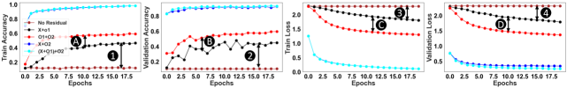
Figure 8. Training Results of all residual configurations with $\textbf{2}\times\textbf{2}$ Kernel.

Our experiments reveal that adding residual connections consistently enhances both training and validation performance, regardless of the specific residual configuration. This is demonstrated in Figure 7 (label to ), where configurations like $X+O1$ perform better that no residual configuration, even though both provide access only to the second quanvolutional layer’s gradients.

Notably, configurations allowing gradient access to both quanvolutional layers, such as $O1+O2$, significantly surpass those with gradient access limited to only one layer, such as $X+O1$, labeled as to in Figure 7. Among all tested configurations, $X+O2$ and $(X+O1)+O2$ showed the best performance. Despite $X+O2$ and $X+O1$ both accessing gradients only from the second quanvolutional layer, $X+O2$ outperformed $X+O1$, primarily due to the influential role of the final classical layer which directly receives the (classical) input data through a skip connection, and hence overshadows the learning contributions of quanvolutional layer(s).

Moreover, $(X+O1)+O2$, which allows gradient flow through both quanvolutional layers, also exhibited superior performance compared to $O1+O2$, which also permits gradient propagation through both layers. This suggests that the classical layer’s influence is significant in $(X+O1)+O2$ configuration also, as it indirectly receives considerable amount of input data via the quanvolutional layers, similar to the $X+O2$ configuration.

Comparison with benchmark models.

To assess the impact of the classical layer in various residual configurations of QuNNs, we conducted a detailed analysis using benchmark models. These models replicated the residual configurations as in label of Figure 5, with one key difference: the quanvolutional layers were made untrainable, keeping their weights fixed, while only the classical layers were trained. This method allowed us to determine the extent to which the classical layer dominates learning, compared to the quanvolutional layers, across all configurations.

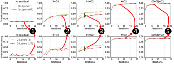
Figure 9. Comparison of ResQuNNs with benchmark model for $\textbf{2}\times\textbf{2}$ Kernel.. T=Trainable, UT=UnTrainable

The benchmark models were trained using the same parameters and dataset as detailed in Section 3. Their training outcomes were then compared with models where both quanvolutional and classical layers were trainable. This comparison, illustrated in Figure 9, highlighted the learning contributions of classical and quantum layers in various residual settings. The observed performance trends in these models offered insights into the effectiveness of quanvolutional layers in different configurations. The key findings from this comparative analysis are summarized below:

No Residual Configuration and X+O1: In these configurations the gradients are accessible only for the second quanvolutional layer. We observed that the model’s performance closely aligns with that of the benchmark models, where quanvolutional layers are not trained. This observation, marked by labels and in Figure 9, can be attributed to the fact that, although both quanvolutional layers are subjected to training, but since the gradients of only the second layer are available whose depth is purposefully set to 1, to have a clear distinction of optimization performance in case of gradient availability across both layers compared to gradient availability in only the last layer, as discussed in Section 2.1. The limited expressiveness of the second layer in such configurations means it does not significantly contribute to learning, becoming overshadowed by the classical layer.

Residual Configuration (O1+O2): In this scenario the gradients are available for both quanvolutional layers, meaning each layer contributes to the learning process. Consequently, we notice a marked improvement in the model’s performance. This becomes particularly evident when comparing with the benchmark model where quanvolutional layers are not trained. As denoted by label in Figure 9, the performance of the model with both quanvolutional layers trained exceeds that of the benchmark by approximately 30%.This improvement underscores the effectiveness of leveraging both quanvolutional layers when gradients are backpropagated through both the layers.

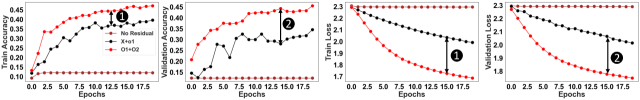
Figure 10. Training Results with $\textbf{3}\times\textbf{3}$ Kernel.

Residual Configuration with Direct/Indirect Input to Classical Layer (X+O2 and (X+O1)+O2): In configurations where the input is either directly or indirectly fed to the classical layer at the network’s end, such as in X+O2 and (X+O1)+O2, the performance of the model with trainable quanvolutional layers mirrors that of the benchmark models. This observation is emphasized by labels and in Figure 9, indicating the predominant role of the classical layer in the learning process. However, considering the enhanced performance in the O1+O2 configuration, which also allows gradient flow through all quanvolutional layers, it suggests that (X+O1)+O2 could be effective in scenarios without a classical layer at the end. This is because it also allows gradient propagation across all quanvolutional layers, potentially enhancing the learning when the classical layer’s dominance is removed.

4.1.2. $\textbf{3}\times\textbf{3}$ Kernel

To investigate the impact of deeper quantum layers, we extended our experiments by training ResQuNNs with two quanvolutional layers, each using a $3\times 3$ kernel, resulting in 9-qubit quanvolutional layers, and are trained on the same dataset and the same set of parameters as discussed in Section 3.

It is worth noting that, in light of our previous findings, where the classical layer dominance was evident in X+O2 and (X+O1)+O2 residual configurations, we do not present the results of these configurations for better visualization of the results. The training results of other residual configurations are shown in Figure 10.

Our experiments showed that models without residual connections demonstrate little to no learning. However, introducing residual connections significantly improved the performance, as depicted in Figure 10. Notably, the O1+O2 residual configuration significantly outperforms the X+O1 setting, as indicated by labels and in the figure. This underscores the importance of enabling gradient flow across all network layers for effective optimization and improved performance. Additionally, it’s noteworthy that although the X+O1 and O1+O2 configurations achieve similar training accuracies, O1+O2 achieved higher validation accuracy, suggesting that direct input data propagation might lead to data memorization, whereas gradient flow throughout the network enhances generalization. These findings underscore the crucial role of residual connections and gradient accessibility in the training and generalization of deeper QuNN architectures.

4.2. Three Quanvolutional Layers

In previous sections, we established the critical importance of gradient accessibility across all layers in QuNNs for achieving better training performance. In this section, we extend our exploration to demonstrate that our proposed ResQuNNs can further facilitate the utilization of an increased number of quanvolutional layers.

Specifically, we consider the scenario of training QuNNs with three quanvolutional layers. In a prior discussion (Figure 3), we illustrated the case of No Residual in three quavolutional layers, revealing that gradients were only available for the final quanvolutional layer. Here, we examine the gradient results for various possible residual settings in the context of three quanvolutional layers. Due to space constraints, we opt to present results only for residual configurations where gradients are accessible across all three quanvolutional layers, as shown in Figure 11. Out of 15 potential residual configurations examined, only two, specifically (O1+O2)+O3 and ((X+O1)+O2)+O3, allowed gradient access across all three layers. The other configurations restricted gradient flow to one or two layers. This further underscores the significance of our proposed residual approach, as it enables the desired comprehensive gradient accessibility, with greater number of qubits, which can be pivotal for optimizing complex problems.

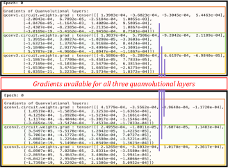
Figure 11. Gradients Propagation Through the Network for Three Quanvolutional Layers for ((X+O1)+O2)+O3 (left) and (O1+O2)+O3 (right)

5. Conclusion

This paper introduces a significant advancement in the field of quanvolutional neural networks (QuNNs) by introducing trainable quanvolutional layers, thereby enhancing the adaptability and feature extraction capabilities of QuNNs. We address the challenges associated with making multiple quanvolution layers trainable, which typically involve limited gradient access throughout the network, with gradients being exclusively available for the last layer. To address this challenge, we propose a novel architecture called Residual Quanvolutional Neural Networks (ResQuNNs), which incorporates residual blocks to effectively tackle the issue of gradient accessibility in QuNNs with multiple quanvolutional layers. This approach not only enhances the trainability of these networks but also optimizes their overall performance. Furthermore, we conduct an empirical investigation into the strategic placement of residual blocks within these networks, leading to valuable insights. We identify specific configurations that facilitate efficient gradient flow across all layers, underscoring the critical role of residual block placement in maximizing network efficiency.

The implications of our work extend beyond theoretical advancements; it opens the door to practical applications in quantum computing and deep learning. ResQuNNs provide a robust framework for harnessing the potential of quantum computing in complex computational tasks, and lays the foundation for future innovations in quantum deep learning, with the potential to revolutionize various domains reliant on advanced computational techniques.

References

- (1)
- Baek et al. (2022) H. Baek et al. 2022. Scalable Quantum Convolutional Neural Networks. arXiv:2209.12372
- Bergholm et al. (2018) V. Bergholm et al. 2018. PennyLane: Automatic differentiation of hybrid quantum-classical computations. arXiv (2018). https://doi.org/10.48550/ARXIV.1811.04968
- Chen et al. (2022) S. Chen et al. 2022. Quantum convolutional neural networks for high energy physics data analysis. Phys. Rev. Res. 4, 1 (2022). https://doi.org/10.1103/PhysRevResearch.4.013231
- Cong et al. (2019) I. Cong et al. 2019. Quantum convolutional neural networks. Nature Physics 15, 12 (2019), 1273–1278. https://doi.org/10.1038/s41567-019-0648-8
- Henderson et al. (2020) M. Henderson et al. 2020. Quanvolutional Neural Networks: Powering Image Recognition with Quantum Circuits. Quantum Machine Intelligence 2, 2 (2020). https://doi.org/10.1007/s42484-020-00012-y
- Hu et al. (2023) M. Hu et al. 2023. Strong quantum nonlocality with genuine entanglement in an -qutrit system. arXiv:2308.16409 [quant-ph]
- Hur et al. (2022) T. Hur et al. 2022. Quantum convolutional neural network for classical data classification. Quantum Mach. Intell 4, 2 (2022). https://doi.org/10.1007/s42484-021-00061-x
- Kashif et al. (2023) M. Kashif et al. 2023. Alleviating Barren Plateaus in Parameterized Quantum Machine Learning Circuits: Investigating Advanced Parameter Initialization Strategies. arXiv 2311.13218 (2023).
- Kashif and Al-kuwari (2024) M. Kashif and S. Al-kuwari. 2024. ResQNets: A Residual Approach for Mitigating Barren Plateaus in Quantum Neural Networks. EPJ Quant. Tech 11, 4 (2024). https://doi.org/10.1140/epjqt/s40507-023-00216-8
- Kim et al. (2023) J. Kim et al. 2023. Classical-to-quantum convolutional neural network transfer learning. Neurocomputing 555 (2023). https://doi.org/10.1016/j.neucom.2023.126643
- Matic et al. (2022) A. Matic et al. 2022. Quantum-classical convolutional neural networks in radiological image classification. In 2022 IEEE International Conference on Quantum Computing and Engineering (QCE). IEEE Computer Society, Los Alamitos, CA, USA, 56–66. https://doi.org/10.1109/QCE53715.2022.00024
- McClean et al. (2018) J. R. McClean et al. 2018. Barren plateaus in quantum neural network training landscapes. Nature Communications 9, 1 (nov 2018). https://doi.org/10.1038/s41467-018-07090-4
- Meedinti et al. (2023) G.N Meedinti et al. 2023. A Quantum Convolutional Neural Network Approach for Object Detection and Classification. arXiv:2307.08204 [quant-ph]
- M.Kashif and Al-Kuwari (2023) M.Kashif and S. Al-Kuwari. 2023. The impact of cost function globality and locality in hybrid quantum neural networks on NISQ devices. Machine Learning: Science and Technology 4, 1 (2023). https://doi.org/10.1088/2632-2153/acb12f
- Rajesh et al. (2021) V. Rajesh et al. 2021. Quantum Convolutional Neural Networks (QCNN) Using Deep Learning for Computer Vision Applications. In 2021 RTEICT. 728–734. https://doi.org/10.1109/RTEICT52294.2021.9574030
- Schuld and Killoran (2019) M. Schuld and N. Killoran. 2019. Quantum Machine Learning in Feature Hilbert Spaces. Physical Review Letters 122, 4 (feb 2019). https://doi.org/10.1103/physrevlett.122.040504
- Sebastian et al. (2023) A. Sebastian et al. 2023. Beyond Qubits : An Extensive Noise Analysis for Qutrit Quantum Teleportation. arXiv:2309.12163 [quant-ph]
- Shen et al. (2023) G. Shen et al. 2023. Quantum convolutional neural network for image classification. Pattern Anal Applic 26 (2023). https://doi.org/10.1007/s10044-022-01113-z
- Wei et al. (2022) S. Wei et al. 2022. A quantum convolutional neural network on NISQ devices. AAPPS Bulletin 32, 2 (2022). https://doi.org/10.1007/s43673-021-00030-3
- Zaman et al. (2023) K. Zaman et al. 2023. A Survey on Quantum Machine Learning: Current Trends, Challenges, Opportunities, and the Road Ahead. arXiv:2310.10315 [quant-ph]