A comparison of next-generation turbulence profiling instruments at Paranal

Abstract

A six-night optical turbulence monitoring campaign has been carried at Cerro Paranal observatory in February and March, 2023 to facilitate the development and characterisation of two novel atmospheric site monitoring instruments - the ring-image next generation scintillation sensor (RINGSS) and 24-hour Shack Hartmann image motion monitor (24hSHIMM) in the context of providing optical turbulence monitoring support for upcoming 20-40m telescopes. Alongside these two instruments, the well-characterised Stereo-SCIDAR and 2016-MASS-DIMM were operated throughout the campaign to provide data for comparison. All instruments obtain estimates of optical turbulence profiles through statistical analysis of intensity and wavefront angle-of-arrival fluctuations from observations of stars. Contemporaneous measurements of the integrated turbulence parameters are compared and the ratios, bias, unbiased root mean square error and correlation of results from each instrument assessed. Strong agreement was observed in measurements of seeing, free atmosphere seeing and coherence time. Less correlation is seen for isoplanatic angle, although the median values agree well. Median turbulence parameters are further compared against long-term monitoring data from Paranal instruments. Profiles from the three small-telescope instruments are compared with the 100-layer profile from the stereo-SCIDAR. It is found that the RINGSS and SHIMM offer improved accuracy in characterisation of the vertical optical turbulence profile over the MASS-DIMM. Finally, the first results of continuous optical turbulence monitoring at Paranal are presented which show a strong diurnal variation and predictable trend in the seeing. A value of 2.65$\arcsec$ is found for the median daytime seeing.

1 Introduction

Atmospheric optical turbulence (OT) induces both phase distortion and amplitude modulation of light that propagates through it, leading to a severe reduction in achievable image quality from ground-based optical instruments. Large astronomical telescopes typically employ adaptive optics (AO) systems to compensate for the wavefront phase distortion, however there is a need for external monitoring of OT during the design, validation and commissioning of such systems. Additionally, knowledge of the vertical distribution of optical turbulence will be crucial for predicting and verifying the performance of multi conjugate adaptive optics (MCAO) systems planned for 20-40m ELT-class telescopes (Costille & Fusco, 2011; Tokovinin, 2010). These systems will therefore demand instruments that measure both "integrated" parameters relevant to AO and the vertical distribution of optical turbulence. Turbulence monitoring instruments are today installed at many of the largest astronomical observatories, providing real-time measurements of turbulence conditions, ensuring that observational sensitivity requirements are met (Milli et al., 2019), and providing long-term site monitoring data which is highly desirable in the development of new optical instruments. Turbulence monitoring is also seen as increasingly important in improving the accuracy of meso-scale turbulence forecasting models (Masciadri et al., 2020), which offer further gains in efficiency for observation scheduling through the process of auto-regression (Masciadri et al., 2023) and will be highly beneficial to the operation of ELT-class instruments. The current standard, small-telescope OT monitoring instruments - the Multi Aperture Scintillation Sensor (MASS) and Differential Image Motion Monitor (DIMM)- are limited by the use of outdated CCD cameras, custom-manufactured equipment and, in the case of the MASS, a noted discrepancy in measurements of OT profiles compared to the high-resolution Stereo-Scintillation Detection and Ranging (S-SCIDAR) technique (Masciadri et al., 2014; Lombardi & Sarazin, 2016). There is therefore significant motivation to develop new instruments based on modern technologies for deployment alongside ELTs.

The minimum requirement for such instruments is firstly accurate measurement of the astronomical seeing $\varepsilon_{0}$. This parameter is directly related to the integrated turbulence strength of the atmosphere and represents the angular size of the seeing-limited (long-exposure) point spread function (PSF) for astronomical observations. The free atmosphere seeing, $\varepsilon_{0,f}$ is a measure of the seeing above an altitude of 500m (Lawrence et al., 2004) and enables a comparison of seeing decoupled from highly localised turbulence in the ground layer. Additional integrated turbulence parameters of interest include the coherence time, $\tau_{0}$, and isoplanatic angle, $\theta_{0}$ (Roddier, 1981). These are relevant to the operation of AO systems, representing respectively an upper limit on the time taken to measure and correct wavefront distortions and an upper limit of the achievable angular correction. MCAO and laser tomographic adaptive optics (LTAO) systems planned for ELT-instruments will also require knowledge of the optical turbulence profile, as do forecasting models, in order to provide meaningful validation of techniques. Accurate measurement of the optical turbulence profile is therefore also highly desirable.

Multi-instrument campaigns have been hosted a number of times at the European Southern Observatory (ESO) Paranal site, including for example Dali Ali et al. (2010) and Osborn et al. (2018). This work details the results from the most recent campaign at Paranal, in which three turbulence profiling instruments based on portable telescopes: the 24-hour Shack-Hartmann image motion monitor (24hSHIMM) (Griffiths et al., 2023), full aperture scintillation sensor (FASS) (Guesalaga et al., 2021) and ring-image next generation scintillation sensor (RINGSS) (Tokovinin, 2021) were compared with permanently installed OT profiling instruments at the site. The primary motivation being to facilitate the development and characterisation of these next-generation instruments against existing techniques. The three instruments were co-located on the northernmost part of the observatory for 6 nights starting on the 27th of February, with the final night of observation on the 5th of March 2023. The ESO Multi Aperture Scintillation Sensor - Differential Image Motion Monitor (MASS-DIMM) (Chiozzi et al., 2016) was operating throughout all nights of observation whereas the stereo-SCIDAR (Osborn & Sarazin, 2018) was operated from the 28th to the 5th only. As a part of the VLT Atmospheric Site Monitoring (ASM) package, measurements of local meteorological parameters were available for additional analysis.

This work will outline the theoretical operating principle behind each instrument used in the campaign and present the major results from the campaign with discussion. The generalised FASS instrument is still under development and so its results have been excluded from this work. The measurements of the 24hSHIMM and RINGSS will be compared directly with the permanent instrumentation - the DIMM, MASS-DIMM and the S-SCIDAR- both on measurements of integrated parameters and on OT profiles using high-resolution vertical $C_{n}^{2}$ profiles obtained from the S-SCIDAR.

2 Turbulence profiling instruments

The concepts and capabilities of each of the instruments used during the campaign are briefly summarised below. For this campaign, the other ESO turbulence profiling instruments: the robotic Slope Detection and Ranging (SLODAR) instrument and the adaptive optics facility on UT-4, were not operational and so are omitted.

2.1 Stereo-SCIDAR

S-SCIDAR, which is described in detail in Shepherd et al. (2014), is a triangulation technique that exploits observations of binary stars with a similar magnitude, requiring a telescope larger than 1-m diameter and low-noise camera due to the relative faintness of such targets, to measure the vertical distribution of OT in the atmosphere. The S-SCIDAR projects the pupil image from each star onto a separate CCD detector using a prism which yields sensitivity advantages over the typical SCIDAR implementation where the pupil images are overlapped on a single camera (Fuchs et al., 1998). The cross covariance of the spatial intensity fluctuations in the two pupil images is analysed to extract a high-resolution optical turbulence $C_{n}^{2}(h)\>\mathrm{d}h$ profile comprised of 100 layers at 250m intervals. Additionally, by analysing the temporal evolution of the cross-covariance responses, it is possible to extract the wind velocity and direction of individual turbulent layers which enables estimation of the optical turbulence coherence time. The S-SCIDAR system at Paranal is mounted on one of the 1.8m auxiliary telescopes and has been extensively tested and validated against existing instrumentation at the site (Osborn et al., 2018). The S-SCIDAR data from this experiment has been processed using the latest corrections for finite spatial sampling described by Butterley et al. (2020a) which also includes subtraction of localised turbulence within the dome.

2.2 DIMM

The DIMM (Sarazin & Roddier, 1990) consists of a small telescope with a CCD camera and a pupil-plane mask of two small circular apertures. Using a prism, the beams from the two apertures are imaged onto a detector and spatially separated. The seeing is measured by analysing the variance in differential position of the two focal spots (Tokovinin, 2002). The DIMM is a simple, portable OT monitor and provides measurements of the seeing at one minute intervals. The Very Large Telescope (VLT) DIMM at Paranal is configured in a combined MASS-DIMM system mounted on a 28-cm Celestron C11 telescope and was installed as a part of the 2016 ASM upgrade on a 7-m tower. Limitations of the instrument include insensitivity to the bias introduced by optical propagation and only providing measurements of the seeing.

2.3 MASS

The MASS (Kornilov et al., 2003) is similarly based around a small-telescope and measures the normalised intensity fluctuations resulting from propagation though turbulence, commonly referred to as the scintillation index, in 4 concentric apertures. Using the theory described by Tokovinin et al. (2003), weighting functions are generated for the 10 (4 normal and 6 differential) scintillation indices at vertical heights of 0, 0.5, 1, 2, 4, 8, 16 km and an inversion algorithm is used to reconstruct the $C_{n}^{2}(h)\,\mathrm{d}h$ of each layer. The VLT MASS is combined in a MASS-DIMM configuration (Kornilov et al., 2007). As the MASS relies solely on measurements of scintillation, it is insensitive to ground-layer turbulence which can be accounted for using simultaneous measurements from the DIMM. The techniques described by Kornilov (2011) allow for estimation of the OT coherence time by measurement of the atmospheric second moment of wind and combination with the DIMM data.

2.4 RINGSS

RINGSS is a solid-state turbulence profiler developed to replace the technically obsolete MASS instruments (Tokovinin, 2021). It uses a 5-inch Celestron telescope where image of a bright single star is optically transformed into a ring. This is achieved by combination of spherical aberration and defocus in the focal-reducer lens. The pixel scale is 1.57 arcsec and the ring radius is 11 pixels. Cubes of 2000 ring images of 48$\times$48 pixel format and 1 ms exposure time are recorded by a CMOS camera. Image processing consists in centering the rings and computing 20 harmonics of intensity variation along the ring (in the angular coordinate). Variances of these harmonics, averaged over 10 image cubes, are related to the turbulence profile by means of weighting functions in the same way as in MASS. RINGSS delivers turbulence integrals in eight layers at 0, 0.25, 0.5, 1… 16 km heights. The results refer to zenith; they are corrected for the finite exposure time bias and partially corrected for deviations from the weak-scintillation regime (saturation). The atmospheric time constant is determined by the method of Kornilov (2011). The instrument operates robotically. Its control provides for selection and change of targets, pointing and centering, and closed-loop focus control.

Scintillation signals in RINGSS are sensitive to the ground-layer turbulence because the image is not focused (analogue of a generalized SCIDAR). Alternative estimation of seeing is made using radial distortions of the rings, like in a DIMM. This "sector" seeing agrees reasonably well with the scintillation-based seeing: the ratio of their mean values is 1.038, the correlation coefficient is 0.97, and the rms scatter around the regression line is 0.11^′′. Under excellent conditions, the sector seeing is systematically larger; this bias appears when turbulence in the ground layer is less than $2\times 10^{-13}$ m^1/3 and is absent otherwise. We attribute this effect to imperfect focusing of the ring in the radial direction, analogous to the similar bias in a defocused DIMM. In the following analysis, we use only the scintillation-based seeing measured by RINGSS, while the supplementary data provide the alternative "sector" seeing values as well.

2.5 24hSHIMM

The 24hSHIMM (Griffiths et al., 2023) is based around a Shack-Hartmann wavefront sensor (SHWFS) and portable 11-inch telescope design. It observes single, bright stars and measures both the intensity and wavefront angle-of-arrival (AoA) fluctuations in each of the SHWFS focal spots. The spatial statistics of the scintillation are compared with weighting functions (Robert et al., 2006) and a non-negative least squares algorithm is used to reconstruct a low-resolution $C_{n}^{2}(h)\,\mathrm{d}h$ profile. The 24hSHIMM is not negatively-conjugated, therefore a scintillation-based reconstruction is insensitive to the ground layer and integrated turbulence strength measurements from SHWFS AoA fluctuations are used to overcome this limitation. The 24hSHIMM is designed to operate for 24-hours a day, typically through use of an InGaAs camera operating in the short-wave infrared to reduce sky background light and minimise the effects of strong turbulence. The 24hSHIMM utilises the FADE method (Tokovinin et al., 2008) to estimate the coherence time of the atmospheric turbulence. This method of direct measurement of coherence time is an improvement on the previous implementation using wind-speed profiles from the ERA5 ECMWF forecast (Hersbach et al., 2020) which are limited by low spatial and temporal resolution. Another notable change from the original implementation of the 24hSHIMM is that in this work, measurements are obtained by a CMOS camera and a 600nm longpass filter which introduces additional constraints on performance.

2.6 Campaign details

The location of each instrument on the Paranal observatory platform is shown in figure  1. The 24hSHIMM and RINGSS were mounted on concrete pillars adjacent to the 1998 DIMM tower within 2m of one-another. The FASS was mounted on a tripod slightly further away, between the old-DIMM tower and SLODAR crate. The 24hSHIMM was mounted approximately 2m off of the ground, the RINGSS and FASS were at about 1.5m. Wind breaks were set up along the Northern fence next to the instruments.

The local environments for the S-SCIDAR and MASS-DIMM are therefore significantly different; they are both much further away from any large buildings and more elevated from the ground. The MASS-DIMM is on a 7 m tower and the S-SCIDAR was mounted on VLTI auxiliary telescope two; the alt-az altitude axis of which is 5-m above surface (Koehler & Flebus, 2000). We therefore expect poorer agreement in the seeing between these instruments and the monitors located near the VLT Survey Telescope (VST), as local turbulence conditions are likely to differ significantly.

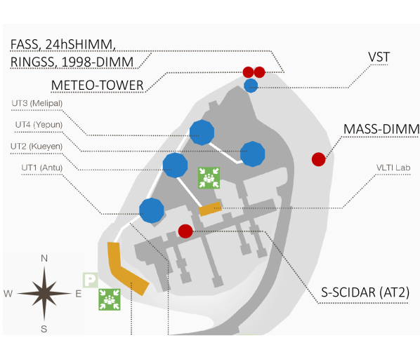
Figure 1: Location of turbulence monitoring instrumentation described in section 2. Instruments relevant to this study are indicated by red circles. Original image credit: ESO.

The list of targets for the RINGSS was shared at the beginning of the experiment and efforts were made to synchronise target stars where possible between the visiting turbulence monitors. The MASS-DIMM and S-SCIDAR however were using separate target lists.

3 Results

The overall results for this campaign are laid out below. This includes both direct comparison of integrated parameter measurements between the different instruments, and a comparison of optical turbulence profiles with the high-resolution S-SCIDAR. A focus is primarily made on comparison of the developmental instruments 24hSHIMM, RINGSS with the well-characterised and permanently installed S-SCIDAR and MASS-DIMM. However all instruments have been compared where appropriate. The comparison between 24hSHIMM and RINGSS is of interest as the two instruments were co-located, observing similar targets and so are much more likely to agree. The agreement of the S-SCIDAR and MASS-DIMM is also of interest to compare to long-term monitoring results and previous studies.

To generate comparison plots, for the instrument on the x-axis, each measurement has been directly plotted against the nearest measurement from the instrument on the y-axis within a maximum time difference of two minutes. If a corresponding measurement could not be found within two minutes, the data point has been excluded from the plot to minimise the effects of temporal evolution of the turbulence on the comparison. This two minute interval was chosen to match the integration time used by the S-SCIDAR as it was the longest of all the instruments. As the algorithm finds the nearest measurement within the search window and the other instruments all have a cadence of a minute or less, reducing the interval to one minute, for example, was observed to produce almost identical statistical comparison parameters. In each comparison plot, a white dashed line represents the line of perfect agreement between the instruments, and the Pearson correlation coefficient, $r$, bias, $\mathrm{B}$, unbiased root mean square error, $\mathrm{RMSE}$, and mean ratio, $\mathrm{MR}$, of each data set is reported in the top-left of the graph. Mathematical definitions of the latter three parameters may be found in appendix A. These comparison parameters are additionally summarised for each figure in table 2. The colour gradient indicates the density of measurements at each point in the graph with black the lowest and pale yellow the highest. The median values from these findings will also be compared where useful to results from long-term studies on seeing conditions at Paranal with Butterley (2021) reporting the latest S-SCIDAR results and Otarola (2021) the results from the MASS and DIMM. These results can be found in table 1. All integrated turbulence parameter measurements displayed below are derived at zenith and a wavelength of 500 nm. All turbulence profiles are given as a function of vertical height. Finally, the distribution and temporal sequences of $C_{n}^{2}(h)\>\mathrm{d}h$ profiles measured by the instruments will be directly compared with the S-SCIDAR through a binning process to investigate accuracy of OT profile characterisation, and the first results from the 24hSHIMM of 24-hour continuous monitoring of OT at Paranal are presented in full.

Table 1: Median values of parameters obtained during this campaign, marked in the columns as ‘2023’, from all instruments are compared with long-term site monitoring results of Otarola (2021); Butterley (2021) with the column labels ‘long-term’. There are some blank entries which correspond to unavailable data - either because the instrument cannot measure the parameter or there is no source for long-term data. The median values for the 24hSHIMM are calculated excluding data taken during the daytime.

	N Profiles	$\varepsilon_{0}(\arcsec)$		$\varepsilon_{0,f}(\arcsec)$		$\theta_{0}(\arcsec)$		$\tau_{0}$ (ms)
Instrument	2023	Long-term	2023	Long-term	2023	Long-term	2023	Long-term	2023
DIMM	2696	0.71	0.75	-	-	-	-	-	-
MASS-DIMM	2477	-	0.79	0.41	0.40	1.98	2.53	6.14	6.3
S-SCIDAR	611	0.72	0.76	0.46	0.51	2.03	2.62	3.61	5.8
RINGSS	5387	-	1.10	-	0.58		2.46	-	5.8
24hSHIMM	1942	-	0.89	-	-	-	2.35	-	6.4

3.1 Seeing

The astronomical seeing, $\varepsilon_{0}$, describes the angular full-width-at-half-maximum (FWHM), typically measured in units of arcseconds, of the seeing-limited point spread function for long-exposure imaging through optical turbulence. It can be calculated using the Fried parameter $r_{0}$ (Fried, 1966),

$$r_{0}=\left[0.423k^{2}\sec(\gamma)\int^{\infty}_{0}C_{n}^{2}(h)\,\mathrm{d}h\right]^{-3/5},$$ (1)

where $k=2\pi/\lambda$ is the wavenumber, $\lambda$ is the wavelength of the light, $\gamma$ the zenith angle of observation in radians, $h$ the altitude of a turbulent layer in metres, $C_{n}^{2}(h)$ the refractive index structure constant, given in units of $\mathrm{m}^{-2/3}$. The relationship between the Fried parameter and the seeing is then given by

$$\varepsilon_{0}=0.98\frac{\lambda}{r_{0}}.$$ (2)

Accurate measurement of the astronomical seeing is the most fundamental requirement of an optical turbulence monitor as it quantifies the integrated turbulence strength of the atmosphere and directly relates this to the degree of image distortion. Seeing is dynamic, can change rapidly and is highly dependant on location and pointing direction (Tokovinin, 2023) which leads to discrepancies between instruments, even for well-synchronised measurements. Median seeing measurements in table 1 indicate that the two instruments located in the northern end of the site, near to the VST and installed at a lower height above ground, are measuring substantially stronger seeing that the MASS-DIMM and S-SCIDAR. This is most likely due to local turbulence effects. There is however a very strong agreement between the DIMM and S-SCIDAR measurements, and a mean ratio close to 1, despite their separation on the site — but noting their similar height above the ground and isolated locations this is not surprising.

It is known that the local seeing at the 1998-DIMM tower is slightly stronger than the current 2016-MASS-DIMM. The median seeing calculated from several years of measurements with the 1998-DIMM between 2010-01-01 and 2015-05-22 was found to be 0.98$\arcsec$ compared to the 2016-DIMM long term seeing of 0.71$\arcsec$. This supports a location-based argument for some of the discrepancy between the visiting and the ESO instruments. Previous campaigns using the Generalised Seeing Monitor at the same location have found seeing values of 0.88$\arcsec$ (Martin et al., 2000) and 1.07$\arcsec$ (Dali Ali et al., 2010). Additionally, high-resolution profiling of the surface layer carried out by Butterley et al. (2020b) using the surface-layer SLODAR identifies an exponentially decaying turbulence strength with altitude — hence we also expect the higher elevation of the MASS-DIMM and S-SCIDAR to result in lower seeing.

Individual comparisons of seeing measured by each instrument are displayed in figure 2. It is extremely encouraging that all seeing measurements display strong correlation with the minimum of $r=0.70$ for the RINGSS compared with the S-SCIDAR. As expected, due to co-location and overlapping targets, the 24hSHIMM and RINGSS display a very strong correlation of 0.83, however there is a significant bias between the two despite their proximity. A number of factors may contribute to this, including the RINGSS corrections for finite exposure time and partial saturation of scintillation - conditions which would lead to underestimates of fast-moving and high altitude turbulent layers on the 24hSHIMM- there is a also a small height offset between the two with the RINGSS being closer to the ground which could lead to slightly stronger turbulence above the telescope pupil. The correlation between the DIMM and S-SCIDAR is equally strong but with far less bias - the results are also consistent with the long term monitoring as seen in table 1.

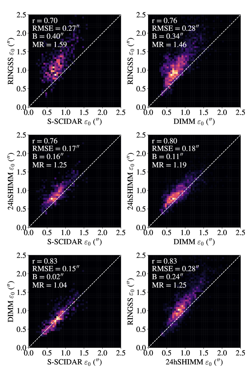
Figure 2: Comparison of contemporaneous seeing measurements during the campaign from the DIMM, S-SCIDAR, 24hSHIMM and RINGSS.

Table 2: Summary of statistical comparison parameters all graphs.

X - axis	Y - axis	r	RMSE	B	MR
Seeing, $\varepsilon_{0}$			($\arcsec$)	($\arcsec$)
S-SCIDAR	RINGSS	0.70	0.27	0.40	1.59
DIMM	RINGSS	0.76	0.28	0.34	1.46
S-SCIDAR	24hSHIMM	0.76	0.17	0.16	1.25
DIMM	24hSHIMM	0.80	0.18	0.11	1.19
S-SCIDAR	DIMM	0.83	0.15	0.02	1.04
24hSHIMM	RINGSS	0.83	0.28	0.24	1.25
Free atmosphere seeing, $\varepsilon_{0,f}$			($\arcsec$)	($\arcsec$)
S-SCIDAR	RINGSS	0.86	0.21	0.14	1.23
MASS-DIMM	RINGSS	0.85	0.22	0.14	1.36
S-SCIDAR	MASS-DIMM	0.80	0.17	-0.03	0.93
Isoplanatic angle, $\theta_{0}$			($\arcsec$)	($\arcsec$)
S-SCIDAR	RINGSS	0.35	0.67	-0.17	0.97
MASS-DIMM	RINGSS	0.40	0.59	-0.08	1.00
S-SCIDAR	24hSHIMM	0.40	0.67	-0.32	0.91
MASS-DIMM	24hSHIMM	0.33	0.65	-0.18	0.96
S-SCIDAR	MASS-DIMM	0.30	0.72	-0.19	0.97
24hSHIMM	RINGSS	0.54	0.53	0.11	1.08
Coherence time, $\tau_{0}$			(ms)	(ms)
S-SCIDAR	RINGSS	0.75	1.94	-0.05	1.00
MASS-DIMM	RINGSS	0.69	3.69	-0.82	0.96
S-SCIDAR	24hSHIMM	0.68	2.15	0.21	1.05
MASS-DIMM	24hSHIMM	0.77	2.46	0.14	1.05
S-SCIDAR	MASS-DIMM	0.70	2.10	0.25	1.05
24hSHIMM	RINGSS	0.80	2.21	-0.53	0.97

3.2 Free atmosphere seeing

The free atmosphere seeing, $\varepsilon_{0,f}$ is calculated as the integrated seeing of all turbulent layers with an altitude of 500 m or greater for the MASS, RINGSS and S-SCIDAR. The 24hSHIMM is limited by a large sub-aperture size of 4.7 cm and cannot sample the highest frequency scintillation fluctuations produced by low-altitude turbulence. This is due to height scaling of the characteristic size of scintillation speckles - given by the radius of the first Fresnel zone, $r\approx\sqrt{\lambda z}$. It therefore lacks the sensitivity required to reconstruct a layer at 500 m, so a direct comparison with the other instruments is not possible and it has been excluded. Figure 3 details the measurements obtained with the three other instruments.

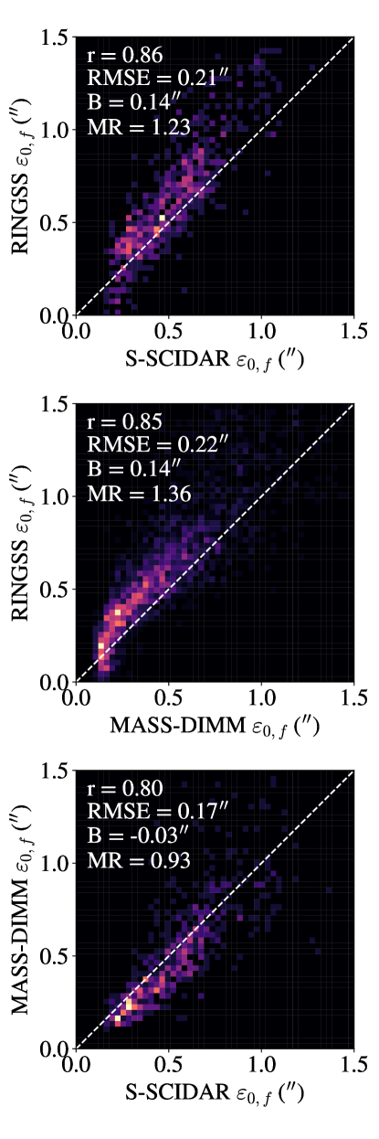
Figure 3: Comparison of contemporaneous free atmosphere seeing measurements during the campaign from the MASS-DIMM, S-SCIDAR, and RINGSS.

3.3 Isoplanatic angle

The isoplanatic angle is defined by Roddier (1981) as

$$\theta_{0}=\left[2.91k^{2}\cos^{-8/3}({\gamma})\int_{0}^{\infty}C_{n}^{2}(h)\,h^{5/3}\mathrm{d}h\right]^{-3/5}.$$ (3)

This quantity is of particular interest for design and operation of AO systems as it represents the separation angle between a guide star and target which will result in 1 rad² RMS wavefront error for phase corrections. It is particularly of interest when considering target availability in single conjugate adaptive optics (SCAO) and in calculation of AO error budgets.

Figure 4 displays the comparisons of isoplanatic angle measured by all instruments. Unlike measurements of the seeing, it is observed that there is less correlation between all instruments. However, the variation of isoplanatic angle during the campaign was small. The strongest correlation, 0.54, is found between 24hSHIMM and RINGSS which observed same targets, while other profilers sampled different turbulent volumes. The $h^{5/3}$ scaling in Eq. 3 implies that this parameter is highly sensitive to turbulence in the upper atmosphere. Therefore an accurate characterisation will require sensitivity to high-altitude turbulence. The 24hSHIMM, RINGSS and MASS are limited in this regard by their response functions for the highest altitude layer which are several kilometres wide. The turbulence distributed over this layer will be averaged and reported at that height, leading to a reduction in accuracy. When taking optical propagation into account for observing at lower zenith angles, saturation of scintillation produced by the highest-altitude layers is an additional source of error for monitors based on weak-scintillation theory. The exception in this experiment being the RINGSS and MASS which implement a correction process. This combination of factors is likely to explain the smaller correlation observed in measurements from the four instruments, while the median values agree fairly closely.

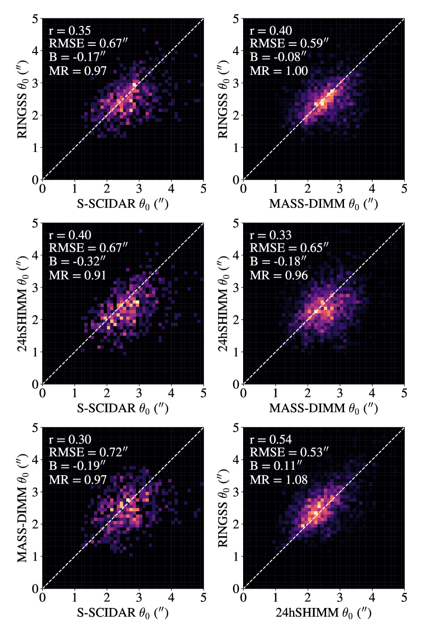
Figure 4: Comparison of contemporaneous isoplanatic angle measurements during the campaign by the MASS-DIMM, S-SCIDAR, 24hSHIMM and RINGSS.

3.4 Coherence time

Knowledge of the coherence time is essential for AO as it defines the minimum bandwidth of the system. The optical turbulence coherence time is typically on the scale of a few ms. It is related to the wind speed profile and turbulence strength in the following way (Roddier, 1981),

$$\tau_{0}=0.314\frac{r_{0}}{\overline{V}_{5/3}},$$ (4)

where $\overline{V}_{5/3}$ is the weighted mean of the wind speed raised to the power of $5/3$,

$$\overline{V}_{5/3}=\left[\frac{\int^{\infty}_{0}V(h)^{5/3}C_{n}^{2}(h)\,\mathrm{d}h}{\int^{\infty}_{0}C_{n}^{2}(h)\,\mathrm{d}h}\right]^{3/5}.$$ (5)

The instruments in this study employ a variety of strategies to measure the coherence time. The S-SCIDAR analyses the spatio-temporal cross-correlations of the scintillation measured in the pupil. Peaks that match atmospheric layers translate across the auto-covariance map with each successive time offset due to translation of the turbulent layers with wind. The direction and speed of each of the layers is recorded and the mean wind speed calculated from Eq. 5. The S-SCIDAR is only able to directly estimate the wind speed of the strongest layers. Weak layers with no detected wind speed are assigned a value through interpolation of the measured wind speed profile. The 24hSHIMM takes a different approach, utilising the FADE method (Tokovinin et al., 2008), which involves fitting response functions, determined by layer wind speeds and $C_{n}^{2}(h)\>\mathrm{d}h$ , to the measured temporal structure function of the Zernike defocus coefficient of the atmospheric wavefront distortions. The 24hSHIMM analysis differs slightly from the FADE instrument as wavefronts are reconstructed by the Shack-Hartmann yielding direct measurements of the Zernike defocus term, and only layer wind speeds need to be fitted. As the 24hSHIMM sampling rate was limited to 100Hz for this experiment, it was necessary to exclude 362 measurements that had a $\overline{V}_{5/3}>15\;\mathrm{ms^{-1}}$ as the defocus structure function curve could not be sampled with a sufficient temporal resolution to fit a wind speed profile. The MASS-DIMM and RINGSS utilise the method described in Kornilov (2011) of including a wind shear component in the weighting functions, continuous exposures without gaps, and a fitting process to estimate the second moment of the wind $\overline{V}_{2}$ with the approximation of $\overline{V}_{2}\approx 1.1\overline{V}_{5/3}$ found by Kellerer & Tokovinin (2007) enabling an estimate of the coherence time.

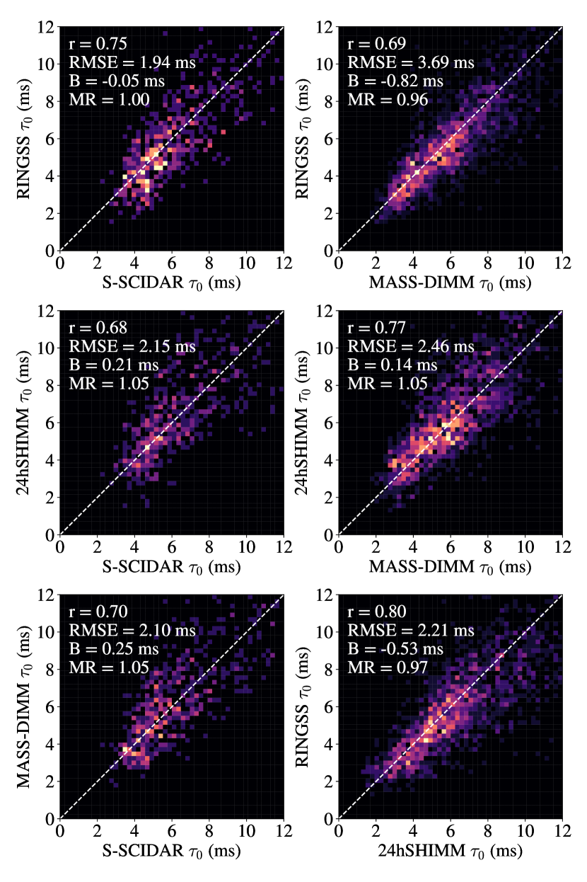
Figure 5: Comparison of contemporaneous measurements of the atmospheric turbulence coherence time by the MASS-DIMM, S-SCIDAR, 24hSHIMM and RINGSS.

Figure 5 displays comparisons of coherence time measurements for the four instruments. The RINGSS and MASS use the same method of calculating coherence time and agree strongly with little bias. The two instruments also agree well with the S-SCIDAR, again with little bias. The 24hSHIMM shows good correlation with all instruments too. The bias however is small but positive with respect to the S-SCIDAR and MASS-DIMM. Lower elevation and imaging through more of the surface layer should lead to a negative bias, suggesting that the instrument may be overestimating coherence time which could be a result of the low frame rate. Finally, the lower correlation of some instruments with the S-SCIDAR may result from the fact that S-SCIDAR measures wind direction and corrects line-of-sight wind speed measurements to the wind speed parallel to the ground, which other instruments cannot do.

3.5 Influence of wind direction

Previous studies have observed that wake produced downwind of large telescope structures can have a significant effect on seeing conditions (Sarazin et al., 1990). Additionally, seeing at the 1998-DIMM tower has historically been stronger than that observed by the UTs for north-easterly and south-easterly winds (Sarazin et al., 2008). A later study by Lombardi et al. (2010) related this phenomenon to an increase in the strength of the surface layer. We therefore expect wind direction to influence the agreement between instruments in this campaign. The wind rose, figure 6, shows the distribution of wind speeds and directions measured 30 m above the ground by the meteo-tower between sunset and sunrise for all six nights of the campaign. The 30 m measurement is used over the 10 m measurement to minimise bias introduced by the Unit Telescopes (UTs) to the South and the VST to the SSW. The radial extent of the bars represents the fraction of the data with a given wind direction and it suggests, similar to previous studies such as Lombardi et al. (2009), that it is mainly from the NNE.

Figure 7 shows how the bias between pairs of instruments changes as a function of wind direction for eight directional bins. In addition, the error bars indicate the bias-corrected RMSE of the comparisons for each wind direction. Due to insufficient data for some wind directions, the correlation is not plotted. Additionally, there were no S-SCIDAR data points between South and West and insufficient data for all instruments for the West bin. These points have therefore been omitted. Seeing measurements during the campaign appear to be strongly influenced by wind direction. For instrument pairs other than the S-SCIDAR and MASS-DIMM, the RMSE of instrument comparisons is larger for northerly winds. The RINGSS bias appears sensitive to the wind direction with the largest bias corresponding to north-westerly winds, but the 24hSHIMM does not follow the same pattern - only seeing a larger bias compared to the MASS-DIMM towards the North-West. However there are few data points for this bin. This figure does not take into account instrument pointing direction, which can also lead to discrepancy in measurements. As this sample of six nights is relatively small, the influence of pointing direction was investigated instead through analysing the median and standard deviation of seeing measured by the 2016-DIMM for all data in the ESO archive. This analysis showed a clear increase in median seeing for north-easterly and south-easterly winds for all pointing angles. Features strongly dependent on pointing angle included: larger variability at low elevation angles when the DIMM points SE and wind blows from the W and SW, and for the DIMM pointing SW while the wind blows from the North. The larger spread of data and bias for northerly winds experienced by the 24hSHIMM and RINGSS may be related to their proximity to the edge of the platform, as shown in figure 1, as air from the ground level will be driven up the mountain and mix with cooler air at the platform. By contrast, wind from the South will traverse the platform before reaching the 24hSHIMM and RINGSS. The S-SCIDAR vs MASS-DIMM seeing comparison has no identifiable dependence on wind direction which is expected as both instruments are raised above the ground and located away from the platform edges and buildings.

For the free atmosphere seeing and isoplanatic angle, dependence on wind direction at 30 m seems unlikely as both parameters are insensitive to ground layer turbulence. In reality, non-Kolmogorov turbulence in the surface layer which may arise from interaction of wind with buildings or heat sources can “confuse” turbulence monitoring instruments that expect a specific power spectrum (typically Von Karman or Kolmorogov), thus leading to inaccuracies in the characterisation of the turbulence profile that may depend on wind direction. Such effects are also encountered at low wind speeds and have been identified at the site by the SLODAR (Butterley et al., 2020b). Figure 6 shows that for southerly winds, a wind speed of less than 3 ms^-1 is proportionally more frequent. For the coherence time, which is also dependent on the vertical wind speed profile, the biases are small relative to the spread of the data, except for the SW which may result from a small number of samples. The wind direction does not seem to have a significant influence on the bias or RMSE of these comparisons, however there is a trend towards a larger negative bias for most instrument comparisons in the NE to SW section of the graph. A full treatment of wind directional discrepancies at Paranal would require a significantly larger data set and is beyond the scope of this study.

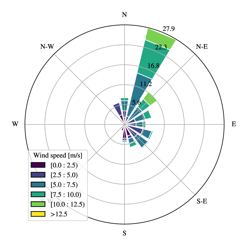
Figure 6: A wind rose displaying the distribution of wind speeds and directions measured 30 m above the ground by the Paranal meteo-tower for the six nights of the campaign.

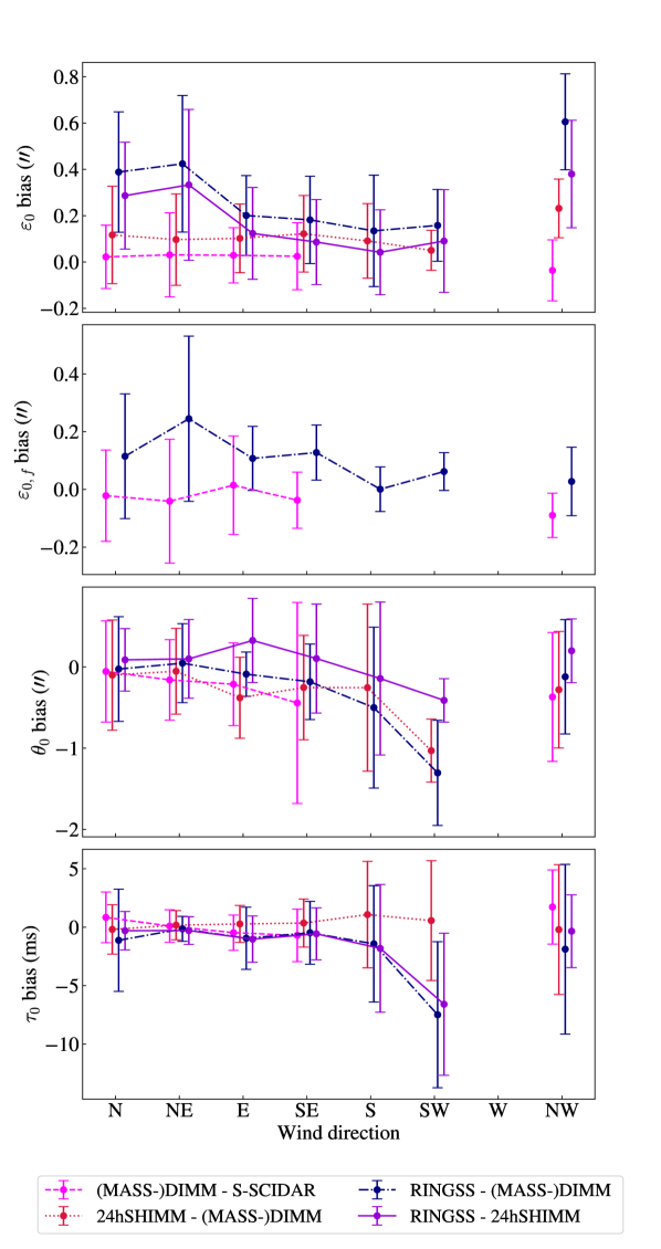
Figure 7: A plot showing the bias of measurements for all four integrated turbulence parameters, and the RMSE indicated by the error bars, as a function of wind direction for key pairs of instruments compared in this study. For the seeing, only DIMM data is used, but for other parameters the MASS-DIMM results use the same line style. The legend indicates the Y - X instrument pair for which the bias and RMSE have been plotted.

3.6 Optical turbulence profiles

Optical turbulence profiles are characterised by the refractive index structure constant $C_{n}^{2}$ as a function of vertical height above the ground. The instruments in this study record the sum of $C_{n}^{2}$ over a given volume $\mathrm{d}h$ for each layer using an inversion process. To facilitate a comparison between all instruments which use different models and layers, the RINGSS, MASS-DIMM and 24hSHIMM are directly compared with the high-resolution S-SCIDAR profiles through binning using instrument response functions.

The response functions dictate the measured $C_{n}^{2}(h)\>\mathrm{d}h$ response to a single, thin turbulent layer placed at any height throughout the atmosphere. These functions are typically evaluated in simulation by passing a single, thin layer from the ground to the upper atmosphere and plotting the $C_{n}^{2}(h)\>\mathrm{d}h$ measured by the instrument in each altitude bin. For scintillation-based instruments such as RINGSS, S-SCIDAR and MASS the response functions usually manifest as triangles on a log scale of height, centred on the altitude of the turbulent layer reconstructed and crossing adjacent bins at half of the input turbulence strength (Tokovinin et al., 2003; Tokovinin, 2021).

Figure 8: A plot of the response functions for the 24hSHIMM and RINGSS. The alternating line styles differentiate the response functions of each reconstructed layer. The sum of responses from all layers is approximately one.

For the 24hSHIMM, this approximation also holds well, except for between the ground layer and the first layer. The response functions $f_{i}(h)$ for the 24hSHIMM and RINGSS are displayed in figure 8 on a linear scale of height. These instruments, as well as MASS, estimate turbulence strength in discrete layers as $C_{n}^{2}(h_{i}){\rm d}h=\int f_{i}(h)C_{n}^{2}(h)\rm{d}h$. The response functions for the MASS can be found in Kornilov et al. (2003).

Figure 9 displays a box and whisker plot of optical turbulence profile measurements from the 24hSHIMM, RINGSS and MASS-DIMM compared with contemporaneous S-SCIDAR profiles. The S-SCIDAR profiles have been binned down to the instrument layers using the response functions and only data within $\pm 2$ minutes of an S-SCIDAR measurement have been used. The whiskers represent the 5th and 95th percentiles of the distribution, the median is shown as a dashed black line and the mean as a solid magenta line. It is therefore possible to simultaneously compare mean profiles and distributions of measurements in individual layers. Figure 9 indicates that all instruments measure a significantly stronger ground layer than the equivalent S-SCIDAR measurement.

A notable feature of the MASS-DIMM profile is a significant underestimation in the 8 km layer, which appears to be the driving cause of the smaller value of median free-atmosphere seeing. For RINGSS and the 24hSHIMM, some layers register zero $C_{n}^{2}(h)\>\mathrm{d}h$ , hence anomalous boxes and whiskers such as the 4km layer for the 24hSHIMM and 2 km layer in RINGSS on a a log-scale of $C_{n}^{2}(h)\>\mathrm{d}h$ . Mean values however agree well for the free-atmosphere layers.

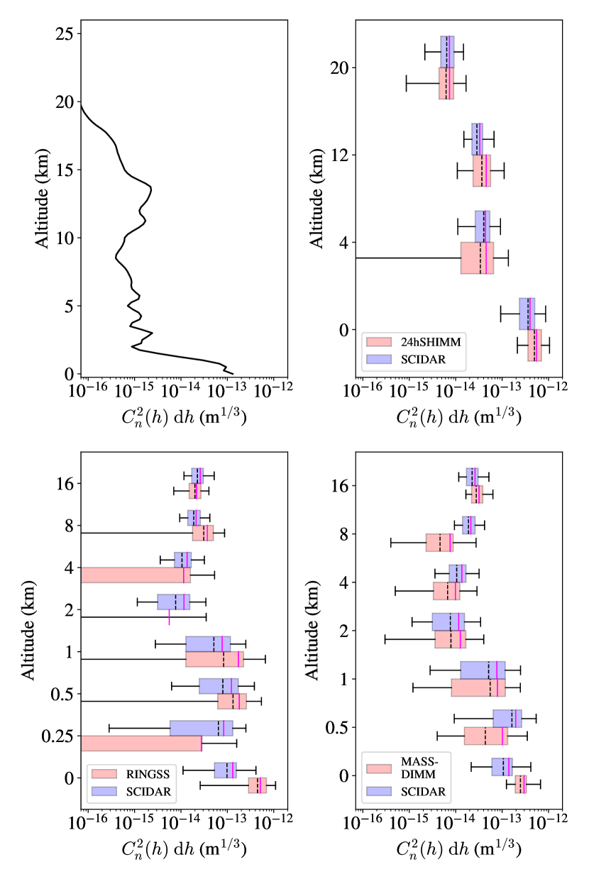
Figure 9: A comparison of $C_{n}^{2}(h)\>\mathrm{d}h$ profile measurements for all instruments with contemporaneous measurements from the S-SCIDAR. The red boxes show the instrument data from each fitted layer, and the adjacent blue boxes the contemporaneous measurements (within +/- two minutes) from the S-SCIDAR which have been binned to match the instrument layers using the response functions. The extent of coloured boxes represents the first and third quartiles, the dashed line the median measurement, the magenta line the mean, and the whiskers the fifth and 95th percentiles of the distribution. From top left to bottom right, the plot shows the mean S-SCIDAR profile, and box and whisker plots for the 24hSHIMM, RINGSS and MASS-DIMM compared with S-SCIDAR. Significantly smaller values in the top-left panel, compared to other panels, are explained by the thinner ${\rm d}h=0.25$ km layers of the S-SCIDAR profiles.

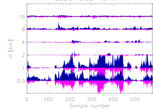
Figure 10: Turbulence profiles measured simultaneously by RINGSS (up-facing blue bars) and S-SCIDAR (down-facing magenta bars). S-SCIDAR is matched in resolution and time to RINGSS with the sample number indicating the nth S-SCIDAR measurement taken during the campaign. The width of each band is $5\times 10^{-13}\mathrm{m}^{1/3}$.

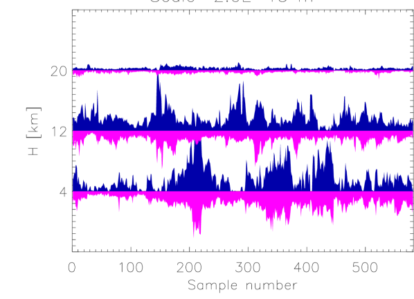
Figure 11: Turbulence profiles measured simultaneously by 24hSHIMM (up-facing blue bars) and S-SCIDAR (down-facing magenta bars). S-SCIDAR is matched in resolution and time to 24hSHIMM with the sample number indicating the nth S-SCIDAR measurement taken during the campaign. The width of each band is $2\times 10^{-13}\mathrm{m}^{1/3}$.

Figure 10 shows a detailed comparison between vertical turbulence profiles measured by RINGSS with all 611 available S-SCIDAR profiles matched in time and resolution. Despite different locations and different target sources, we note a strong agreement of timing and localisation of strong turbulence packets, especially in the 0.5 and 1-km layers. The ground layer is not included in this comparison. Figure 11 shows a similar plot for the 24hSHIMM. It suggests that the correlation between lower-altitude layers is higher than for high-altitude layers, evidencing the low correlation in isoplanatic angle.

3.7 Day and night measurements

The 24hSHIMM measures OT profiles continuously for 24-hours a day by operating at short-wave infrared wavelengths. Compared to the visible light, this extends the validity of the weak-scintillation assumption and reduces the sky background. Additional techniques for rapid background subtraction (Griffiths et al., 2023) are also employed to ensure accurate photometry.

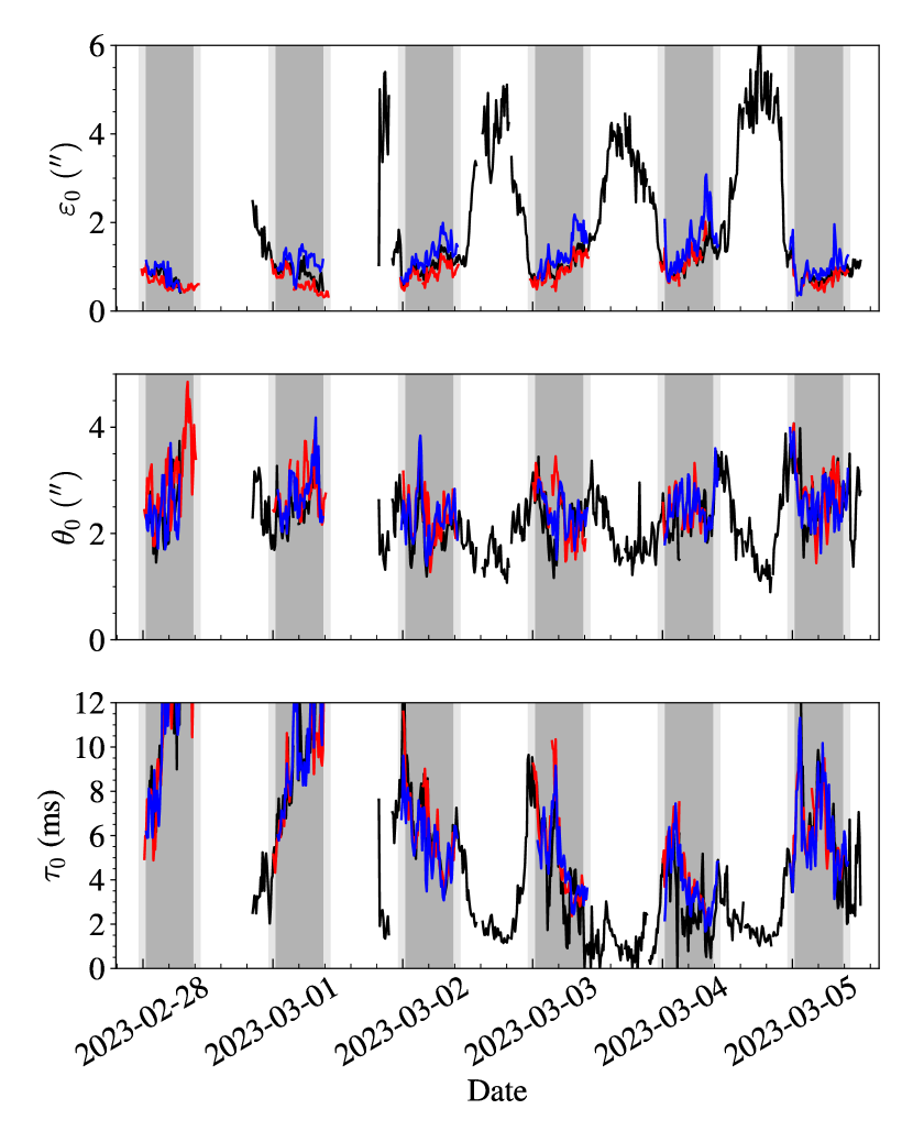
Figure 12: Integrated parameters measured by the 24hSHIMM during the campaign. The black line represents 24hSHIMM measurements, the red line DIMM measurements for seeing and MASS-DIMM for the coherence time and isoplanatic angle, and the blue line the RINGSS. All data sets have been binned to 10-minute intervals for presentation and dates are in UTC. The white, grey and light grey shades of the background represent daytime, night and twilight respectively

Figure 12 shows a continuous plot of the three main integrated turbulence parameters estimated by the 24hSHIMM: seeing, isoplanatic angle and coherence time. Because the instrument produced a measurement every 1-2 minutes, for presentation purposes the data have been binned such that each data point represents the average of any measurements that fall into ten-minute bins. The sharp diurnal variation in seeing is immediately evident from the graph, with a repetitive, sharp drop in the seeing after sunset leading to the best conditions in earliest part of the night. The general trend thereafter appears to be a gradual increase in the seeing until just after sunrise where it rises very strongly. More work is needed to understand the underlying processes behind this behaviour and the influence of meteorological parameters.

The median value of the daytime seeing, calculated between sunrise and sunset, was found to be 2.65$\arcsec$, isoplanatic angle 2.05$\arcsec$ and coherence time $2.4$ ms. It is notable that measurements of the isoplanatic angle, which is insensitive to low-altitude turbulence, do not experience the same distinct variation. This suggests that the increased turbulence strength during daytime is a result of solar heating at the ground affecting the boundary layer, and the upper atmosphere is relatively unaffected. The coherence time follows a similar trend to the Fried parameter likely due to dominance of the strong ground layer turbulence.

4 Conclusions

An optical turbulence monitoring campaign has been carried out at Cerro Paranal observatory between the 27th February and 5th March 2023. The aim of this study was to characterise novel turbulence monitoring instruments, the 24hSHIMM and RINGSS, against existing instruments at the site through comparison measurements of vertical OT profiles and integrated parameters including the seeing, free-atmosphere seeing, isoplanatic angle and coherence time.

Data collected from these two instruments during the campaign were further compared against measurements from the S-SCIDAR and the MASS-DIMM by assessing the RMSE, bias and correlation of contemporaneous data from pairs of instrument. Additionally median values from the whole campaign were calculated and compared to long-term averages.

It was found, as in previous campaigns, that the seeing measured near the old 1998-DIMM tower was significantly larger than for the S-SCIDAR and 2016-MASS-DIMM. In general, however, strong correlation was found across all seeing and free-atmosphere seeing measurements. Isoplanatic angle measurements displayed a close agreement in median values, but were less correlated between all instruments, which is likely a result of limitations in sensitivity to high altitude turbulence and differences in the sampled turbulence volumes. Coherence time measurements were strongly correlated between all instruments, however the RMSE of distributions was relatively large. The influence of wind direction on statistical agreement between measurements was also investigated which showed increased spread and bias in RINGSS and 24hSHIMM seeing comparisons with the MASS-DIMM for northerly winds. Additionally, changes in bias for parameters that should have no dependence on the wind direction could be attributed to non-Kolmogorov effects.

The accuracy of OT profiling was also investigated by comparison of profiles with contemporaneous S-SCIDAR measurements binned using instrument response functions. The two visiting instruments were found to agree well with the S-SCIDAR, with expected bias towards stronger turbulence in the ground layer. It was also observed that the MASS-DIMM systematically underestimates the 8 km layer.

Finally, the first measurements of continuous optical turbulence parameters at Paranal were presented which indicate a predictable and extreme diurnal variation in seeing with a median daytime value of 2.65$\arcsec$ compared to equivalent night-time median of 0.88$\arcsec$, which is assumed to be driven by changes in the boundary layer due to solar heating in the early morning and rapid cooling in the evening as similar changes are not present in the isoplanatic angle which is sensitive to high altitude turbulence. This experiment suggests that the best seeing conditions are in the earliest part of the night.

Data Availability

RINGSS, 24hSHIMM and S-SCIDAR data may be found in the accompanying supplementary files. MASS-DIMM data is available from the ESO ASM archive .

Appendix A Statistical comparison parameters

In this section, the equations for statistical comparison parameters used in figures 2-5 and tables 1-2 are defined. In all equations $i={1,2,3\dots N}$ indicates a sample of $N$ independent turbulence parameter measurements, $X_{i}$ the measurement of the parameter by instrument $X$ and $Y_{i}$ the contemporaneous measurement of the parameter by instrument $Y$. The bias, $\mathrm{B}$ is defined as

$$\mathrm{B}=\sum_{i=1}^{N}\frac{Y_{i}-X_{i}}{N},$$ (6)

the root mean square error (with bias subtracted), or $\mathrm{RMSE}$, as

$$\mathrm{RMSE}=\sqrt{\sum_{i=1}^{N}\frac{([Y_{i}-\overline{Y_{i}}]-[X_{i}-\overline{X_{i}}])^{2}}{N}},$$ (7)

where $\overline{Y_{i}},\overline{X_{i}}$ are the means of the contemporaneous measurements, and the mean ratio by

$$\mathrm{MR}=\frac{1}{N}\sum_{i=1}^{N}\frac{Y_{i}}{X_{i}}.$$ (8)

References

- Butterley (2021) Butterley T., 2021, Technical report, SCIDAR reprocessing: part of the MASS reprocessing investigation part 2b. ESO, Durham University
- Butterley et al. (2020a) Butterley T., Sarazin M., Le Louarn M., Osborn J., Farley O. J. D., 2020a, in Schmidt D., Schreiber L., Vernet E., eds, Adaptive Optics Systems VII. SPIE, p. 75, doi:10.1117/12.2562559
- Butterley et al. (2020b) Butterley T., Wilson R. W., Sarazin M., Dubbeldam C. M., Osborn J., Clark P., 2020b, Monthly Notices of the Royal Astronomical Society, 492, 934
- Chiozzi et al. (2016) Chiozzi G., Sommer H., Sarazin M., Bierwirth T., Dorigo D., Vera Sequeiros I., Navarrete J., Del Valle D., 2016. p. 991314, doi:10.1117/12.2232302, http://proceedings.spiedigitallibrary.org/proceeding.aspx?doi=10.1117/12.2232302
- Costille & Fusco (2011) Costille A., Fusco T., 2011, in AO for ELT 2011 - 2nd International Conference on Adaptive Optics for Extremely Large Telescopes.
- Dali Ali et al. (2010) Dali Ali W., et al., 2010, Astronomy & Astrophysics, 524, A73
- Fried (1966) Fried D. L., 1966, Journal of the Optical Society of America, 56, 1372
- Fuchs et al. (1998) Fuchs A., Tallon M., Vernin J., 1998, Publications of the Astronomical Society of the Pacific, 110, 86
- Griffiths et al. (2023) Griffiths R., Osborn J., Farley O., Butterley T., Townson M. J., Wilson R., 2023, Optics Express, 31, 6730
- Guesalaga et al. (2021) Guesalaga A., Ayancán B., Sarazin M., Wilson R. W., Perera S., Le Louarn M., 2021, Monthly Notices of the Royal Astronomical Society, 501, 3030
- Hersbach et al. (2020) Hersbach H., et al., 2020, Quarterly Journal of the Royal Meteorological Society, 146, 1999
- Kellerer & Tokovinin (2007) Kellerer A., Tokovinin A., 2007, Astronomy & Astrophysics, 461, 775
- Koehler & Flebus (2000) Koehler B., Flebus C., 2000. p. 13, doi:10.1117/12.390206, http://proceedings.spiedigitallibrary.org/proceeding.aspx?doi=10.1117/12.390206
- Kornilov (2011) Kornilov V., 2011, Astronomy & Astrophysics, 530, A56
- Kornilov et al. (2003) Kornilov V., Tokovinin A. A., Vozyakova O., Zaitsev A., Shatsky N., Potanin S. F., Sarazin M. S., 2003, in Wizinowich P. L., Bonaccini D., eds, Adaptive Optical System Technologies II. p. 837, doi:10.1117/12.457982, http://proceedings.spiedigitallibrary.org/proceeding.aspx?doi=10.1117/12.457982
- Kornilov et al. (2007) Kornilov V., Tokovinin A., Shatsky N., Voziakova O., Potanin S., Safonov B., 2007, Monthly Notices of the Royal Astronomical Society, 382, 1268
- Lawrence et al. (2004) Lawrence J. S., Ashley M. C., Tokovinin A., Travouillon T., 2004, Nature, 431
- Lombardi & Sarazin (2016) Lombardi G., Sarazin M., 2016, Monthly Notices of the Royal Astronomical Society, 455
- Lombardi et al. (2009) Lombardi G., Zitelli V., Ortolani S., 2009, Monthly Notices of the Royal Astronomical Society, 399, 783
- Lombardi et al. (2010) Lombardi G., et al., 2010. p. 77334D, doi:10.1117/12.856772, http://proceedings.spiedigitallibrary.org/proceeding.aspx?doi=10.1117/12.856772
- Martin et al. (2000) Martin F., Conan R., Tokovinin A., Ziad A., Trinquet H., Borgnino J., Agabi A., Sarazin M., 2000, Astronomy and Astrophysics Supplement Series, 144
- Masciadri et al. (2014) Masciadri E., Lombardi G., Lascaux F., 2014, Monthly Notices of the Royal Astronomical Society, 438, 983
- Masciadri et al. (2020) Masciadri E., Martelloni G., Turchi A., 2020, Monthly Notices of the Royal Astronomical Society, 492, 140
- Masciadri et al. (2023) Masciadri E., Turchi A., Fini L., 2023, Monthly Notices of the Royal Astronomical Society, 523, 3487
- Milli et al. (2019) Milli J., et al., 2019, in AO4ELT 2019 - Proceedings 6th Adaptive Optics for Extremely Large Telescopes.
- Osborn & Sarazin (2018) Osborn J., Sarazin M., 2018, Monthly Notices of the Royal Astronomical Society, 480, 1278
- Osborn et al. (2018) Osborn J., et al., 2018, Monthly Notices of the Royal Astronomical Society, 478, 825
- Otarola (2021) Otarola A., 2021, Technical report, Paranal Observatory site: Long-term statistics of optical turbulence, PWV and meteorological conditions. ESO
- Robert et al. (2006) Robert C., Conan J.-M., Michau V., Fusco T., Vedrenne N., 2006, Journal of the Optical Society of America A, 23, 613
- Roddier (1981) Roddier F., 1981, Progress in Optics, 19, 281
- Sarazin & Roddier (1990) Sarazin M., Roddier F., 1990, Astronomy and Astrophysics, 227, 294
- Sarazin et al. (1990) Sarazin M., et al., 1990, Technical report, VLT Report 62. ESO
- Sarazin et al. (2008) Sarazin M., Melnick J., Navarrete J., Lombardi G., 2008, The Messenger
- Shepherd et al. (2014) Shepherd H. W., Osborn J., Wilson R. W., Butterley T., Avila R., Dhillon V. S., Morris T. J., 2014, Monthly Notices of the Royal Astronomical Society, 437, 3568
- Tokovinin (2002) Tokovinin A., 2002, Applied Optics, 41, 957
- Tokovinin (2010) Tokovinin A., 2010, in 1st AO4ELT conference - Adaptive Optics for Extremely Large Telescopes. EDP Sciences, Les Ulis, France, p. 02005, doi:10.1051/ao4elt/201002005, http://ao4elt.edpsciences.org/10.1051/ao4elt/201002005
- Tokovinin (2021) Tokovinin A., 2021, Monthly Notices of the Royal Astronomical Society, 502, 794
- Tokovinin (2023) Tokovinin A., 2023, Atmosphere, 14, 1694
- Tokovinin et al. (2003) Tokovinin A., Kornilov V., Shatsky N., Voziakova O., 2003, Monthly Notices of the Royal Astronomical Society, 343, 891
- Tokovinin et al. (2008) Tokovinin A., Kellerer A., Coudé Du Foresto V., 2008, Astronomy & Astrophysics, 477, 671