Semi-Supervised Diffusion Model for Brain Age Prediction

Abstract

Brain age prediction models have succeeded in predicting clinical outcomes in neurodegenerative diseases, but can struggle with tasks involving faster progressing diseases and low quality data. To enhance their performance, we employ a semi-supervised diffusion model, obtaining a 0.83(p<0.01) correlation between chronological and predicted age on low quality T1w MR images. This was competitive with state-of-the-art non-generative methods. Furthermore, the predictions produced by our model were significantly associated with survival length (r=0.24, p<0.05) in Amyotrophic Lateral Sclerosis. Thus, our approach demonstrates the value of diffusion-based architectures for the task of brain age prediction.

1 Introduction

Brain age prediction refers to the task of predicting an individual’s age using neuroimaging data [1]. As individuals age, various brain structures and functions degrade; which lead to negative health outcomes [2, 3, 4, 5, 6, 2, 7]. These changes do not occur at the same rate across people, such that individuals may have the same chronological age but different brain ages [8]. This disparity is particularly present in neurodegenerative diseases such as: Alzheimer’s Disease (AD) and Multiple Sclerosis (MS). In such diseases, an older appearing brain has been associated with: disease status, higher risk of mortality, the speed of disease progression, and disease related genetic markers [9, 10, 11, 12].

However, the brain age paradigm has seen limited application to amyotrophic lateral sclerosis (ALS) [13]. ALS, is one of the rarest and fastest progressing neurodegenerative diseases; with a median survival time (time from diagnosis to death) of only 3 years [14]. With such a short time-window for the most significant ageing related brain changes to occur, effective brain age models for ALS need to be particularly sensitive to ageing related neuroanatomical changes. One study demonstrated that individuals with cognitive and behavioural symptoms but not motor impairment have an association with a higher brain age; this further outlines the subtlety of the relationship between neuroanatomical ageing and ALS [13]. Additionally, brain age models are often trained on high quality (research grade) data, which reduces their wider applicability in real-world settings where the quality of data is lower (clinical grade); this is particularly true for rare diseases like ALS.

Generative models may offer a solution, as they have demonstrated great capabilities in capturing latent factors within an image (e.g., ageing) and produce representations which are robust to data quality [15, 16, 17, 18, 19, 20, 21, 22]. In particular, diffusion models have demonstrated image synthesis capabilities well beyond previous approaches [23, 24, 25].

In this work, we present a novel brain age prediction architecture which leverages the representation learning capabilities of diffusion autoencoders [17]. Our approach produces representations which are robust to data quality, and conditioned on the neuroanatomical effects of ageing. This results in predictions which are accurate on clinical-grade data and associated with mortality in ALS disease at a level which surpasses non-generative approaches.

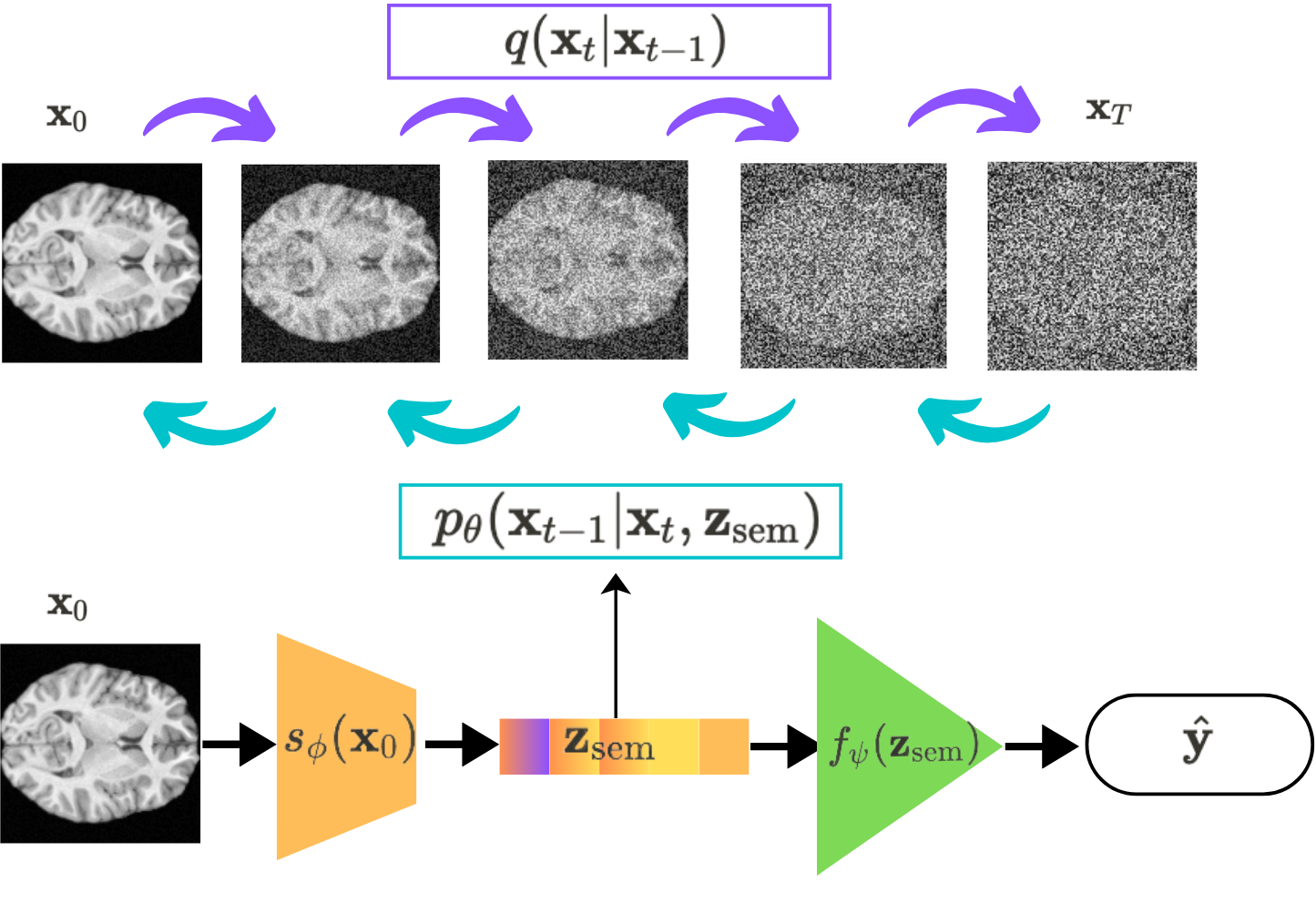
Figure 1: The Model architecture. First the image, $\mathbf{x}_{0}$ goes through the forward process $q(\mathbf{x}_{1:T}|\mathbf{x}_{0})$, to produce $\mathbf{x}_{T}$. The reverse process, $p_{\theta}(\mathbf{x_{0:T}}|\mathbf{z}_{\text{sem}})$ then reconstructs the image conditioned on the semantic latent, produced by $s_{\phi}(\mathbf{x}_{0})$. Finally, the age predictor, $f_{\psi}(\mathbf{z}_{\text{sem}})$ predicts an individual’s age, $\hat{\mathbf{y}}$.

2 Background

2.1 Diffusion Models

Diffusion models allow us to approximate a data distribution, $q(\mathbf{x}_{0})$, with a learnt distribution, $p_{\theta}({\mathbf{x}}_{0})$, via a latent variable model which takes the form:

$$p_{\theta}(\mathbf{x}_{0})=\int p_{\theta}(\mathbf{x}_{0:T})d\mathbf{x}_{1:T},\quad\text{where}\quad p_{\theta}(\mathbf{x}_{0:T}):=p_{\theta}(\mathbf{x}_{T})\prod_{t=1}^{T}p_{\theta}^{(t)}(\mathbf{x}_{t-1}|\mathbf{x}_{t})$$ (1)

Where the latents $\mathbf{x}_{1},...,\mathbf{x}_{T}$ share the same dimensions as our training data $\mathbf{x}_{0}\sim q(\mathbf{x}_{0})$ [15, 16, 26]. As denoted above, the transitions between latents are defined as a Markov chain beginning at a prior $p(\mathbf{x}_{T})=\mathcal{N}(\mathbf{x}_{T};\textbf{0},\textbf{I})$ and ending at our model distribution $p_{\theta}(\mathbf{x}_{0})$. We call this joint distribution, $p_{\theta}(\mathbf{x}_{0:T})$, the reverse process. In contrast to most latent variable models, the approximate posterior $q(\mathbf{x}_{1:T}|\mathbf{x}_{0})$ is predefined as another Markov chain, that we call the forward process. This process destroys the structure of our data, $\mathbf{x}_{0}$, via the gradual addition of Gaussian noise, defined as:

$$q(\mathbf{x}_{1:T}|\mathbf{x}_{0}):=\prod^{T}_{t=1}q(\mathbf{x}_{t}|\mathbf{x}_{t-1}),\quad\text{where}\quad q(\mathbf{x}_{t}|\mathbf{x}_{t-1}):=\mathcal{N}(\mathbf{x}_{t};\sqrt{1-\beta_{t}}\mathbf{x}_{t-1},\beta_{t}\textbf{I})$$ (2)

Where $\beta_{1},...,\beta_{T}$ are scalars which enforce a variance schedule. The reverse process, $p_{\theta}(\mathbf{x}_{0:T})$, denoises our image following the forward process, $q(\mathbf{x}_{1:T}|\mathbf{x}_{0})$, to recover our data distribution. Our model, $p_{\theta}({\mathbf{x}}_{0})$, may be trained by minimising a variational lower bound on negative log likelihood:

$$\mathbb{E}\left[-\log p_{\theta}(\mathbf{x}_{0})\right]\leq\mathbb{E}_{q}\left[-\log\frac{p_{\theta}(\mathbf{x}_{0:T})}{q(\mathbf{x}_{1:T}|\mathbf{x}_{0})}\right]=\mathbb{E}_{q}\left[-\log p_{\theta}(\mathbf{x}_{0:T})-\log q(\mathbf{x}_{1:T}|\mathbf{x}_{0})\right]$$ (3)

At time $t$, the approximate posterior is another Gaussian, $q(\mathbf{x}_{t}|\mathbf{x}_{0})=\mathcal{N}(\sqrt{\alpha_{t}}\mathbf{x}_{0},(1-\alpha_{t})\mathbf{I})$, where $\alpha_{t}=\prod_{s=1}^{t}(1-\beta_{s})$. Thus, the noised image at time $t$ can be expressed as $\mathbf{x}_{t}=\sqrt{\alpha_{t}}\mathbf{x}_{0}+\sqrt{1-\alpha_{t}}\epsilon$ where $\epsilon\sim\mathcal{N}(\mathbf{0},\mathbf{I})$. This allows us to simplify our objective, by learning a model, $\epsilon_{\theta}^{(t)}(\mathbf{x}_{t})$, which predicts the sampled noise, $\epsilon$, based on $\mathbf{x}_{t}$ and $t$. This holds provided that our noised image at time $t$ is assumed to be Gaussian with a fixed variance according to $\alpha_{t}$ and a learnable mean admitting the following loss (see [16] for the full derivation):

$$L:=\sum_{t=1}^{T}\mathbb{E}_{\mathbf{x}_{0}\sim q(\mathbf{x}_{0}),\epsilon_{t}\sim\mathcal{N}(\mathbf{0},\mathbf{I})}\left[\|\epsilon_{\theta}^{(t)}(\sqrt{\alpha_{t}}\mathbf{x}_{0}+\sqrt{1-\alpha_{t}}\epsilon_{t})-\epsilon_{t}\|^{2}_{2}\right]$$ (4)

Table 1: Results of brain age prediction. The first three rows are different metrics demonstrating the accuracy of the brain age predictions on an external dataset. The final row is the relationship (again Pearson’s r) between the brain-PADs and survival in months (time from scan to death) on ALS patients. Significant relationships are displayed in bold.

	Our Model	DenseNet 121[27]	brainageR[28]	DeepBrainNet[29]
Test R	0.83(p<0.001)	0.83(p<0.001)	0.46(p<0.001)	0.81(p<0.001)
Test MAE	5 years	8.63 years	11.7 years	5.55 years
Test R2	0.65	0.12	-1.14	0.56
ALS Survival	0.24(p<0.05)	-0.05 (p=0.61)	0.17 (p=0.14)	-0.12 (p=0.28)

Table 2: Results of Two-Sample Kolmogorov-Smirnov tests for significance between the PADs produced by our model and those produced by other models. Significant results are displayed in bold.

	Our Model	DenseNet 121[27]	brainageR[28]	DeepBrainNet[29]
Mean	-6.19	-1.60	-19.17	-1.13
Std	27.29	7.74	10.97	8.06
KS Statistic		0.32(p<0.05)	0.47(p<0.001)	0.31(p<0.05)

2.2 Diffusion Autoencoders

Diffusion autoencoders modify diffusion models by conditioning the reverse process on a latent, $\mathbf{z}_{\text{sem}}\in\mathbb{R}^{d}$ where $\mathbf{x}_{0}\in\mathbb{R}^{D}$ and $d\ll D$. This latent is output by a semantic encoder, $s_{\phi}({\mathbf{x}_{0}}):\mathbb{R}^{D}\rightarrow\mathbb{R}^{d}$, that is distinct from our noise predictor, $\epsilon_{\theta}^{t}(\mathbf{x}_{t})$. The modified reverse process takes the form:

$$p(\mathbf{x}_{0:T}|\mathbf{z_{\text{sem}}})=p(\mathbf{x}_{T})\prod_{t=1}^{t=T}p(\mathbf{x}_{t-1}|\mathbf{x}_{t},\mathbf{z_{\text{sem}}})$$ (5)

By conditioning the reverse process on a semantic latent, diffusion autoencoders force the stochasticity contained within the image to be modelled by our forward process, $q(\mathbf{x}_{t}|\mathbf{x}_{0})$ [17]. Whilst the semantically meaningful information is forced into our latent $\mathbf{z}_{\text{sem}}$, this leads to rich representations which allow for accurate predictions in the present context.

3 Method

Our model fuses a diffusion autoencoder with an age predictor network, $f_{\psi}(\mathbf{z}_{\text{sem}}):\mathbb{R}^{d}\rightarrow\mathbb{R}^{+}$ which predicts an individual’s age based on the latent representation, $\mathbf{z}_{\text{sem}}$ of their brain image, $\mathbf{x}_{0}$. The model takes as input a batch of images sampled from a dataset $q(\mathcal{X})=\bigl{\{}\mathbf{x}_{0,i}\bigl{\}}_{i=1}^{N}$ where $\mathbf{x}_{0,i}\in\mathbb{R}^{D}$. The images are accompanied by age labels, $\mathcal{Y}=\bigl{\{}\mathbf{y}_{i}\bigl{\}}$, where $\mathbf{y}_{i}\in\mathbb{R}^{+}$. First the image, $\mathbf{x}_{0}$, goes through the forward process, $q(\mathbf{x}_{1:T}|\mathbf{x}_{0})$, to produce $\mathbf{x}_{T}$. The reverse process, $p_{\theta}(\mathbf{x}_{0:T}|\mathbf{z}_{\text{sem}})$, then reconstructs the image conditioned on the semantic latent, $\mathbf{z}_{\text{sem}}$, produced by $s_{\phi}({\mathbf{x}_{0}})$. Finally, the age predictor, $f_{\psi}(\mathbf{z}_{\text{sem}})$ predicts an individual’s age; see Figure 1 for visual intuition.

Our objective is a sum of two MSE losses. The first loss is modified version of Equation 4. With the addition that the noise predictor $\epsilon_{\theta}$ also takes as input $\mathbf{z}_{\text{sem}}$, at every time step. Whilst the second loss is the standard MSE between predicted age and actual age:

$$L_{AGE}=\frac{1}{N}\sum^{N}_{i=0}(\mathbf{y}_{i}-\hat{\mathbf{y}_{i}})^{2}$$ (6)

Thus, the model receives direct supervision from the labels learnt by $f_{\psi}(\mathbf{z}_{\text{sem}})$ and receives self-supervision via its generative arm, learnt by $p_{\theta}(\mathbf{x}_{0:T}|\mathbf{z}_{\text{sem}})$ making for a semi-supervised diffusion model. The model is also semi-supervised in the classic sense of the term as unlabelled are used when training to help condition our latent space. In those instances the image is run through the model in the usual fashion without producing an age prediction $f_{\psi}(\mathbf{z}_{\text{sem}}$).

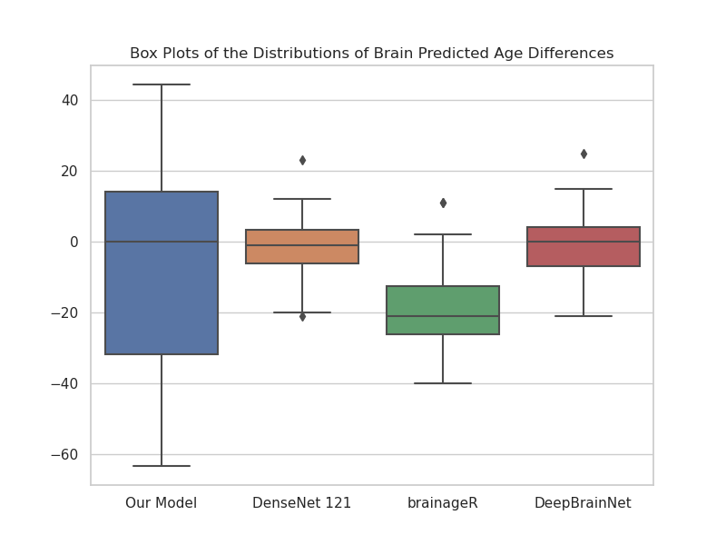
Figure 2: A Boxplot of the distribution of brain-PADs produced by different models on our ALS dataset. Our model produces more variation within the brain-PADs of the ALS patients. Two-Sample Kolmogrov Smirnov tests (Table 2) demonstrated that our brain-PADs were significantly different from brain-PADs from the other three approaches .

4 Results

We trained our model on $4631$ 2D T1w Magnetic Resonance Imaging (MRI) scans from $8$ publicly available datasets (mean age = $56$ years, std = $20.9$ years). For more details concerning the datasets and pre-processing see Appendix B; for details concerning the network design and hardware see Appendix C. Our test set comprised 473 2D T1w MR images (mean age = 68 years, std = 10 years), 100 % of which were clinical grade.

We achieved a test accuracy 0.83(p<0.01) measured as the Pearson’s r correlation coefficient between predicted and chronological age (MAE = 5 years, $\text{R}^{2}=0.65$). Table 1 displays our performance compared to state-of-the-art brain age prediction methods, which demonstrates that we are competitive with these approaches. The final row of Table 1 shows the correlation between the brain predicted age difference (measured as predicted age minus chronological age) and survival in months in our ALS patient group. This quantity is the biomarker typically used to characterise accelerated ageing [2, 1].

The brain predicted age differences (brain-PADs) produced by our model are significantly correlated with survival in months for 72 patients with ALS disease (mean age = 61 years, std = 10.9 years). The other standard approaches did not produce brain-PADs which were significantly associated with this outcome. Table 2 shows that the brain-PADs produced by our method were significantly different from the rest of the techniques; see Figure 2 for visual intuition.

5 Discussion

In this work, we present a novel diffusion based brain age prediction architecture. To our knowledge, this is the first application of a class of diffusion model to this task. Our results demonstrate that our approach is competitive with state-of-the-art brain age prediction models on a dataset completely composed of clinical-grade data. It exhibited a modest improvement over existing techniques, achieving the joint highest Pearson correlation coefficient (r = 0.83, p < 0.01), the highest coefficient of determination ($\text{R}^{2}$ = 0.65), and the lowest mean absolute error (MAE) of 5 years.

Most importantly, the ALS brain-PADs produced by our method also capture more variance than non-generative approaches in a statistically significant way; as displayed in the box plots shown in Figure 2. This variation in brain-PADs was also significantly associated with survival time in ALS, unlike non-generative approaches. This demonstrates that our method is sensitive to the subtle relationship between ALS derived neuroanatomical changes and the ageing process. We posit that our improved performance can be attributed to the capacity of diffusion based architectures, to produce representations which are well conditioned on latent factors within an image, (e.g., the neuroanatomical effects of ageing) and robust to data quality.

6 Future Work and Limitations

Although the association between the ALS brain-PADs and survival was significant, the results would be better if the effect size were larger. However, the small sample size of ALS patients ($n=72$) certainly contributed to this. It is also interesting to note that the mean of the brain-PADs was negative ($-6.19$ years), which is the opposite direction of what is expected. Future work should use larger cohorts of ALS patients to see if the effect size of the association between PADs and survival increases; as well as whether the brain-PADs remain mainly negative. The model may also be augmented by including a separate ALS survival objective; but this of course requires more patient data. It may also be extended to process 3D data and should be tested on other diseases such as: AD and MS. We leave this to future work, and treat the present study as a preliminary exposition of our approach to brain age prediction.

7 Related Work

Choi et al. [30] used a variational autoencoder to model age conditioned brain topography using positron emission tomography data. The authors found that as they aged individuals with the model, their predicted regional metabolic changes, were associated with their actual follow-up changes. However, this approach was not able to make age predictions as age was required in-order to use the model.

Mouches et al. [31] used an age conditioned autoencoder coupled with a brain age regressor, to produce a model which can produce synthetic brain images of a particular age and perform brain age predictions.

Zhao et al. [32] similarly combined an age regressor with a variational autoencoder, to model age conditioned latent’s whilst producing brain age predictions. Although both approaches also used MRI data, they were not applied to a patient dataset, so the significance of their approaches for disease groups is unknown. Additionally they were trained solely on research-grade data so are unlikely to generalise to clinical-grade scans.

8 Acknowledgements

This work was supported by funding from the Engineering, and Physical Sciences Research Council (EPSRC), the UCL Centre for Doctoral Training in Intelligence, Integrated Imaging in Healthcare (i4health) and the Motor Neuron Disease (MND) Association.

9 Checklist

1. For all authors…

   1. Do the main claims made in the abstract and introduction accurately reflect the paper’s contributions and scope? [Yes]

   2. Did you describe the limitations of your work? [Yes] see 6.

   3. Did you discuss any potential negative societal impacts of your work? [Yes] see A.

   4. Have you read the ethics review guidelines and ensured that your paper conforms to them? [Yes].

2. If you are including theoretical results…

   1. Did you state the full set of assumptions of all theoretical results? [N/A]

   2. Did you include complete proofs of all theoretical results? [N/A]

3. If you ran experiments…

   1. Did you include the code, data, and instructions needed to reproduce the main experimental results (either in the supplemental material or as a URL)?[No] This is because although alot of the data is available from public datasets, individuals must apply to the relevant consortiums in order to have access. We have provided much detail concerning the datasets in Appendix B, such that the relevant applications can be made if someone wishes. We have however included code that can be used to train a model, (see the Abstract). This can then be used to make predictions if the data is acquired.

   2. Did you specify all the training details (e.g., data splits, hyperparameters, how they were chosen)? [Yes] see Appendix C

   3. Did you report error bars (e.g., with respect to the random seed after running experiments multiple times)? [N/A]

   4. Did you include the total amount of compute and the type of resources used (e.g., type of GPUs, internal cluster, or cloud provider) [Yes] see Appendix C

4. If you are using existing assets (e.g., code, data, models) or curating/releasing new assets…

   1. If your work uses existing assets, did you cite the creators? [Yes]

   2. Did you mention the license of the assets?[N/A]

   3. Did you include any new assets either in the supplemental material or as a URL? [N/A]

   4. Did you discuss whether and how consent was obtained from people whose data you’re using/curating? [N/A]

   5. Did you discuss whether the data you are using/curating contains personally identifiable information or offensive content? [N/A]

5. If you used crowdsourcing or conducted research with human subjects…

   1. Did you include the full text of instructions given to participants and screenshots, if applicable? [N/A]

   2. Did you describe any potential participant risks, with links to Institutional Review Board (IRB) approvals, if applicable? [N/A]

   3. Did you include the estimated hourly wage paid to participants and the total amount spent on participant compensation? [N/A]

Appendix

Appendix A Potential Negative Societal Impact

Brain age prediction is primarily used in order to make inferences about cognitive and neuroanatomical decline. Although these predictions may aid in: clinical trial design, disease prognostication and classification. One could imagine brain age prediction being used by bad actors to discriminate against an individual based on their brain age. An example would be an insurance company who would offer higher premiums for individuals with older looking brains. With that being said, we anticipate that the clinical utility of this tool outweighs the likelihood of such events occurring.

Appendix B Dataset and Pre-processing

We curated one dataset for the task of standard brain age prediction and a separate dataset for ALS survival analyses. Our brain age prediction dataset consisted of 4621 3D structural T1-weighted MR images for training (mean age=56 years, std=20.9 years) and 473 3D structural T1-weighted MR images for testing (mean age=68 years, std=10 years). All individuals included in training were considered to be radiologically normal (of non-disease status). Our data were drawn from 8 publicly available datasets. These were: the Open Access Series of Imaging Studies-1, the Australian Imaging, Biomarker & Lifestyle Flagship Study of Ageing (AIBL), the Southwest University Adult Lifespan Dataset, the Alzheimer’s Disease Neuroimaging Initiative (ADNI) dataset, the Dallas Lifespan Brain Study, the Nathan Kline Insti- tute Rocklands Sample, the National Alzheimer’s Coordinating Center and the Cambridge Centre for Ageing and Neuroscience study (Cam-CAN). Our ALS dataset comprised 72 3D T1w MR images (mean age = 61 years, std=10.9 years) from the San Rafaele Hospital in Milan. All images underwent the following pre-processing. The ANTS package was used to conduct affine registrations of the images to the MNI 152 brain template, they were then resampled to 130 × 130 × 130 resolution, Simple ITK was used to perform n4 bias field correcttion and HD-BET was used to skull strip the images [33, 34, 35]. 2D medial axial slices were then taken from the 3D volumes, which had their pixel values normalised to be between 0 and 1, after being resized to 128 × 128 resolution.

Appendix C Network Design and Hardware

All model hyperparameters and architectural details were chosen heuristically. Our noise predictor network $\mathbf{\epsilon}^{(t)}_{\theta}$ was a U-Net with the following design. The first convolutional layer expanded the input from a single channel to 32. The tensor stayed at this channel depth for another three convolutional layers. Following this, channel multipliers (2, 3, 4) were applied every 3 convolutional layers making for a channel expansion of (32 → 32 → 32) → (32 → 32 → 32) → (64 → 64 → 64) → (96 → 96 → 96) → (128 → 128 → 128). Three attention blocks then followed, which received a flattened version of the output; this formed the middle block of the U-Net. The upward path of the U-Net was simply the exact reverse of the downward path with regard to channel expansion. Where the channels were equal across the two U-Net paths, a residual connection sent information across. Group normalisation followed each convolutional layer as well as the SiLU activation function. Our semantic encoder network, $\mathbf{s}_{\phi}(\mathbf{x}_{0})$ was the downward path of the U-Net and the middle block. The semantic encoder, output latent representations, $\mathbf{z}_{\text{sem}}$ of dimension $512$. The age predictor network, $\mathbf{f}_{\psi}(\mathbf{z}_{\text{sem}})$, was an MLP which consisted of two linear layers of size: (512 → 128 → 32) following these layers a final layer mapped to the age. Between each layer was a ReLU, batch normalisation and $0.5$ dropout. There were $10.12$ million parameters in total. All training was performed on an Nvidia GeForce RTX 4090 graphics card, with the Adam optimizer using PyTorch lightning [36] all model components $\mathbf{\epsilon}^{(t)}_{\theta}(\mathbf{z}_{\text{sem}})$, $s_{\phi}(\mathbf{x}_{0})$ and $f_{\psi}(\mathbf{z}_{\text{sem}})$ were trained simultaneously.

Appendix D Additional Results

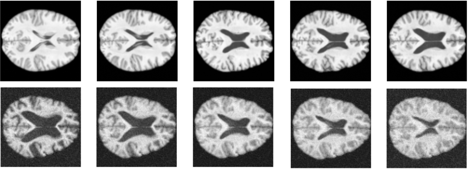
Figure 3: Age Interpolations. In the first row, the image in the first column is that of a 25-year-old, we then linearly interpolate between them and a 75-year-old (final column). The second row is the same but reversed, from age 92 to age 20. The difference in data quality, across the two rows, exemplifies the robustness of the model to varied data quality.

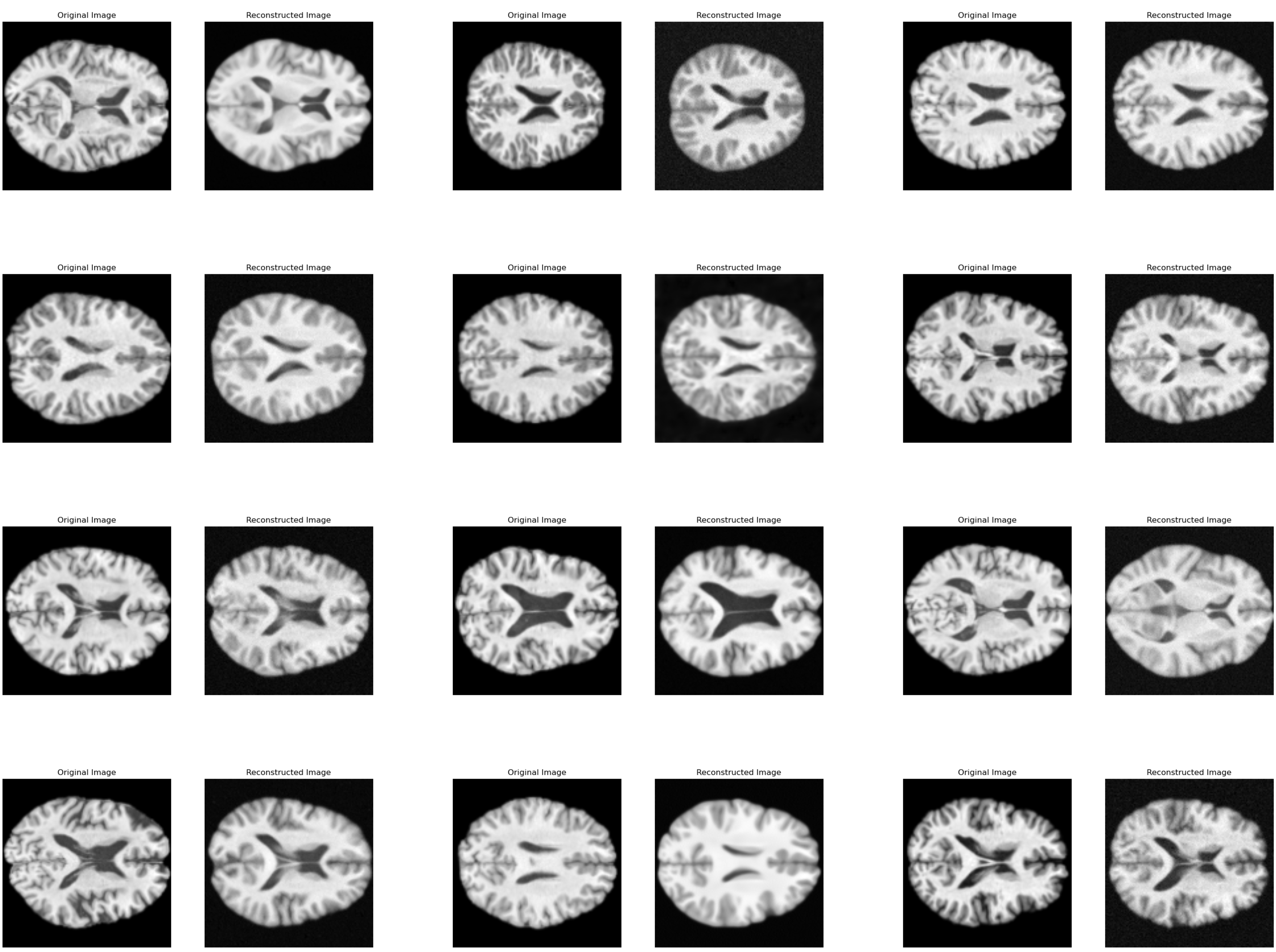
Figure 4: Image Reconstructions. The images on the left columns are the original image, and the images on the right columns are their reconstructed version.

References

- [1] Lea Baecker et al. “Machine learning for brain age prediction: Introduction to methods and clinical applications” In eBioMedicine 72 Elsevier, 2021, pp. 103600 DOI: 10.1016/J.EBIOM.2021.103600
- [2] James H Cole, Riccardo E Marioni, Sarah E Harris and Ian J Deary “Brain age and other bodily ‘ages’: implications for neuropsychiatry” In Molecular psychiatry 24.2 Nature Publishing Group UK London, 2019, pp. 266–281
- [3] Habtamu M Aycheh et al. “Biological brain age prediction using cortical thickness data: a large scale cohort study” In Frontiers in aging neuroscience 10 Frontiers Media SA, 2018, pp. 252
- [4] Lea Baecker et al. “Machine learning for brain age prediction: Introduction to methods and clinical applications” In EBioMedicine 72 Elsevier, 2021
- [5] James H Cole, Robert Leech, David J Sharp and Alzheimer’s Disease Neuroimaging Initiative “Prediction of brain age suggests accelerated atrophy after traumatic brain injury” In Annals of neurology 77.4 Wiley Online Library, 2015, pp. 571–581
- [6] Ann-Marie G De Lange et al. “Multimodal brain-age prediction and cardiovascular risk: The Whitehall II MRI sub-study” In NeuroImage 222 Elsevier, 2020, pp. 117292
- [7] Mark A Eckert “Slowing down: age-related neurobiological predictors of processing speed” In Frontiers in neuroscience 5 Frontiers Research Foundation, 2011, pp. 25
- [8] James H Cole et al. “Brain age predicts mortality” In Molecular psychiatry 23.5 Nature Publishing Group, 2018, pp. 1385–1392
- [9] Maria Ly et al. “Improving brain age prediction models: incorporation of amyloid status in Alzheimer’s disease” In Neurobiology of Aging 87 Elsevier, 2020, pp. 44–48 DOI: 10.1016/J.NEUROBIOLAGING.2019.11.005
- [10] James H. Cole PhD et al. “Longitudinal Assessment of Multiple Sclerosis with the Brain-Age Paradigm” In Annals of Neurology 88.1 John Wiley & Sons, Ltd, 2020, pp. 93–105 DOI: 10.1002/ANA.25746
- [11] Luise Christine Löwe, Christian Gaser and Katja Franke “The Effect of the APOE Genotype on Individual BrainAGE in Normal Aging, Mild Cognitive Impairment, and Alzheimer’s Disease” In PLOS ONE 11.7 Public Library of Science, 2016, pp. e0157514 DOI: 10.1371/JOURNAL.PONE.0157514
- [12] Iman Beheshti, Norihide Maikusa and Hiroshi Matsuda “The association between “Brain-Age Score” (BAS) and traditional neuropsychological screening tools in Alzheimer’s disease” In Brain and Behavior 8.8 John Wiley & Sons, Ltd, 2018, pp. e01020 DOI: 10.1002/BRB3.1020
- [13] Andreas Hermann et al. “Cognitive and behavioural but not motor impairment increases brain age in amyotrophic lateral sclerosis” In Brain Communications 4.5, 2022, pp. fcac239 DOI: 10.1093/braincomms/fcac239
- [14] B Swinnen and W Robberecht “The phenotypic variability of amyotrophic lateral sclerosis” In NATURE REVIEWS | NEUROLOGY 10, 2014, pp. 661–670 DOI: 10.1038/nrneurol.2014.184
- [15] Jonathan Ho, Ajay Jain and P. Abbeel “Denoising Diffusion Probabilistic Models” In ArXiv abs/2006.11239, 2020 URL: https://api.semanticscholar.org/CorpusID:219955663
- [16] Jiaming Song, Chenlin Meng and Stefano Ermon “Denoising diffusion implicit models” In arXiv preprint arXiv:2010.02502, 2020
- [17] Konpat Preechakul, Nattanat Chatthee, Suttisak Wizadwongsa and Supasorn Suwajanakorn “Diffusion Autoencoders: Toward a Meaningful and Decodable Representation” In 2022 IEEE/CVF Conference on Computer Vision and Pattern Recognition (CVPR), 2021, pp. 10609–10619 URL: https://api.semanticscholar.org/CorpusID:244729224
- [18] Calvin Luo “Understanding Diffusion Models: A Unified Perspective” In ArXiv abs/2208.11970, 2022 URL: https://api.semanticscholar.org/CorpusID:251799923
- [19] Jakub M. Tomczak “Deep Generative Modeling” In Deep Generative Modeling, 2022
- [20] Shentong Mo, Zhun Sun and Chao Li “Representation Disentanglement in Generative Models with Contrastive Learning” In 2023 IEEE/CVF Winter Conference on Applications of Computer Vision (WACV), 2023, pp. 1531–1540
- [21] Irina Higgins et al. “beta-VAE: Learning Basic Visual Concepts with a Constrained Variational Framework” In International Conference on Learning Representations, 2016
- [22] Prafulla Dhariwal and Alex Nichol “Diffusion Models Beat GANs on Image Synthesis” In Advances in Neural Information Processing Systems 34, 2021
- [23] Aditya Ramesh et al. “Hierarchical Text-Conditional Image Generation with CLIP Latents” In ArXiv abs/2204.06125, 2022 URL: https://api.semanticscholar.org/CorpusID:248097655
- [24] Robin Rombach et al. “High-Resolution Image Synthesis with Latent Diffusion Models” In 2022 IEEE/CVF Conference on Computer Vision and Pattern Recognition (CVPR), 2021, pp. 10674–10685 URL: https://api.semanticscholar.org/CorpusID:245335280
- [25] “MidJourney” URL: https://www.midjourney.com/
- [26] Jascha Sohl-Dickstein, Eric Weiss, Niru Maheswaranathan and Surya Ganguli “Deep unsupervised learning using nonequilibrium thermodynamics” In International conference on machine learning, 2015, pp. 2256–2265 PMLR
- [27] David A Wood et al. “Accurate brain-age models for routine clinical MRI examinations” In Neuroimage 249 Elsevier, 2022, pp. 118871
- [28] Francesca Biondo et al. “Brain-age is associated with progression to dementia in memory clinic patients” In NeuroImage: Clinical 36 Elsevier, 2022, pp. 103175
- [29] Vishnu M Bashyam et al. “MRI signatures of brain age and disease over the lifespan based on a deep brain network and 14 468 individuals worldwide” In Brain 143.7 Oxford University Press, 2020, pp. 2312–2324
- [30] Hongyoon Choi, Hyejin Kang, Dong Soo Lee and Alzheimer’s Disease Neuroimaging Initiative “Predicting aging of brain metabolic topography using variational autoencoder” In Frontiers in aging neuroscience 10 Frontiers Media SA, 2018, pp. 212
- [31] Pauline Mouches et al. “Unifying Brain Age Prediction and Age-Conditioned Template Generation with a Deterministic Autoencoder” In Proceedings of the Fourth Conference on Medical Imaging with Deep Learning 143, Proceedings of Machine Learning Research PMLR, 2021, pp. 497–506 URL: https://proceedings.mlr.press/v143/mouches21a.html
- [32] Qingyu Zhao et al. “Variational autoencoder for regression: Application to brain aging analysis” In Medical Image Computing and Computer Assisted Intervention–MICCAI 2019: 22nd International Conference, Shenzhen, China, October 13–17, 2019, Proceedings, Part II 22, 2019, pp. 823–831 Springer
- [33] Brian B. Avants, N. Tustison and Hans J. Johnson “Advanced Normalization Tools (ANTs)”, 2020
- [34] Richard Beare, Bradley C. Lowekamp and Ziv Rafael Yaniv “Image Segmentation, Registration and Characterization in R with SimpleITK.” In Journal of statistical software 86, 2018
- [35] M Schell et al. “Automated brain extraction of multi-sequence MRI using artificial neural networks”, 2019 European Congress of Radiology-ECR 2019
- [36] William A Falcon “Pytorch lightning” In GitHub 3, 2019