Abstract

This work develops a Bayesian non-parametric approach to signal separation where the signals may vary according to latent variables. Our key contribution is to augment Gaussian Process Latent Variable Models (GPLVMs) to incorporate the case where each data point comprises the weighted sum of a known number of pure component signals, observed across several input locations. Our framework allows the use of a range of priors for the weights of each observation. This flexibility enables us to represent use cases including sum-to-one constraints for estimating fractional makeup, and binary weights for classification. Our contributions are particularly relevant to spectroscopy, where changing conditions may cause the underlying pure component signals to vary from sample to sample. To demonstrate the applicability to both spectroscopy and other domains, we consider several applications: a near-infrared spectroscopy data set with varying temperatures, a simulated data set for identifying flow configuration through a pipe, and a data set for determining the type of rock from its reflectance.

1 Introduction

We develop a Bayesian non-parametric approach that handles additive models, with an emphasis on signal separation and mixture models. Signal separation considers applications where a single observation is composed of several components and it typically aims to either (i) identify what are the underlying signals Jayaram & Thickstun (2020); Chatterjee et al. (2021) or (ii) estimate the fraction of each signal present Wytock & Kolter (2014); Yip et al. (2022). Mixture models are a class of probabilistic models where each observation comes from a distinct probability distribution Murphy (2022).

As motivation, spectroscopy seeks to identify the abundances of different chemical species $\{c=1,\ldots,C\}$ in a particular sample $i$. Each of the chemical species has a specific pure component signal, $s_{c}$, varying across different wavelengths $\{\lambda_{j}\}_{j=1}^{M}$. The measured signal $d_{ij}$ for sample $i$ at wavelength $\lambda_{j}$ is the weighted sum of the pure component signals, where the weights ($r_{ic}$) correspond to the chemical abundances present in sample $i$. However, the pure component signals in a given sample not only depend on the wavelength but also on other factors, such as temperature or a sample’s crystal structure. Our key idea, and the starting point for this paper, is to use a latent variable $x_{i}$ for each sample to model the sample-specific underlying conditions:

$$d_{ij}=\sum_{c=1}^{C}r_{ic}\;s_{c}(x_{i},\lambda_{j})+\epsilon_{ij},$$ (1)

where $\epsilon_{ij}$ is some noise which is assumed to be Gaussian and $s_{c}(\cdot,\cdot)$ are unknown functions.

Figure 1: Bayesian diagram for mixed-output Gaussian Process latent variable models (MO-GPLVM) with unobserved mixture weights $r_{ic}$.

When combined with the constraints that

$$\sum_{c=1}^{C}r_{ic}=1\;\forall\;i\quad\text{and}\quad r_{ic}\in[0,1]\;\forall\;i,c,$$ (2)

our formulation closely resembles applications in spectroscopy Tauler (1995); Alsmeyer et al. (2004); Kriesten et al. (2008); Muñoz & Torres (2020) and hyper-spectral unmixing Altmann et al. (2013); Borsoi et al. (2019; 2021). When constraints for $r_{ic}$ change from $r_{ic}\in[0,1]$ to $r_{ic}\in\{0,1\}$, Eq. (2) becomes that used for mixture models Ritchie et al. (2020); Manole & Ho (2022); He et al. (2022).

A challenge with allowing the signals $s_{c}(\cdot,\cdot)$ to vary with latent variables $x_{i}$ is that the likelihood can only provide information about the sum of the underlying signals. Since we wish to learn about and disambiguate the multiple, underlying signals, we need regularization to share information between samples. But existing approaches are not applicable in this setting due to new, physically-relevant challenges:

• There is no parametric description of the signals, so we cannot rely on physical models common in spectroscopy Alsmeyer et al. (2004); Dirks & Poole (2019),

• There are relatively few observations of which only a small portion is labeled, meaning that we cannot rely on deep learning Neri et al. (2021); Hong et al. (2021),

• We may not have data on the pure signals $s_{c}$, that is data with all $r_{ic}$ equal 0 except 1 may be unavailable, so we cannot pre-train the model on the pure signals Borsoi et al. (2019); Jayaram & Thickstun (2020).

To simultaneously overcome these challenges, we propose using Gaussian Processes or GPs Williams & Rasmussen (2006) to develop a model that makes principled estimates for its own regularisation by optimizing the Evidence Lower Bound (ELBO). The combined use of Gaussian Processes and latent variables has been widely studied in Gaussian Process Latent Variable Models or GPLVMs Lawrence & Hyvärinen (2005); Titsias & Lawrence (2010); Damianou et al. (2016); Dai et al. (2017); de Souza et al. (2021); Ramchandran et al. (2021); Lalchand et al. (2022). This work extends the GPLVM framework to the case where each data point comprises the weighted sum of a known number of pure component signals.

When only one signal is present in each observation (called mixture model in the rest of this paper), GPLVM-based approaches have been proposed for classifying the observations per categories corresponding to the signal present Urtasun & Darrell (2007); Kazlauskaite et al. (2019); Ahmed et al. (2019); Sharma & Chopra (2020); Jørgensen & Hauberg (2021); Ajirak et al. (2022). These approaches proceed in two steps: fitting a single GPLVM to all observations and then performing classifications based on the latent variables. In contrast, our approach uses a single step, directly encoding the class into our proposed Mixed-Output GPLVM.

In the signal separation setting where multiple signals are present in every data points, GPLVM has been proposed by Altmann et al. (2013) for hyper-spectral imaging. Altmann et al. (2013) use a GPLVM where the latent variables correspond to the unknown mixture fractional weights to capture a specific, physically motivated form of non-linearity. This differs from our approach in two ways. First, our approach incorporates latent variables $x_{i}$ which may be independent of the mixture fractional weights. Second, our prior on the deviation from a linear model which only depends on $x_{i}$ and $\lambda_{j}$ is more flexible.

The next section describes the proposed Mixed-Output Gaussian Process Latent Variable Model (MO-GPLVM) and derives an Evidence Lower Bound (ELBO) for the log-marginal likelihood. Section 3 gives implementation details, Section 4 presents the experiments, and Section 5 concludes.

2 Mixed-Output Gaussian Process Latent Variable Models

Figure 2: Illustrative example of MO-GPLVM: by inputting a set of observed data $(a)$ consisting of training data (top), with known mixture fractions, and test data (bottom), with unknown mixture fractions, MO-GPLVM will produce variational posterior estimates $(b)$ the fractional composition of the test data (top left) and for the latent variables of both the training and the test data (bottom left), and a Gaussian Process estimate, shown with a mean and $95\%$ confidence interval, for the pure component signals for both components, (right).

For this work, we consider a set of data generated according to Equation (1), where each data point $i=1,\dots,N$ is observed at a fixed grid of $j=1,\dots,M$ locations. Figure 1 describes the structure of the model where we use the following notation for the pure component signals:

$$s_{ijc}=s_{c}(x_{i},\lambda_{j})\;.$$ (3)

This paper considers a setting where we have a set of training observations ($D=\{d_{ij}\}\in\mathbb{R}^{N\times M}$) with known weights ($R=\{r_{ic}\}\in\mathbb{R}^{N\times C}$), and a set of test data observations $D^{*}=\{d^{*}_{ij}\}\in\mathbb{R}^{N^{*}\times M}$ for which the weights are unknown. Using this we are interested in learning the posterior for the unknown weights of the test observations, $R^{*}=\{r^{*}_{ic}\}\in\mathbb{R}^{N^{*}\times C}$, the latent variables for the training and test data, denoted by $X=\{x_{i}\}\in\mathbb{R}^{N\times A}$ and $X^{*}=\{x^{*}_{i}\}\in\mathbb{R}^{N^{*}\times A}$ respectively, and the pure component signals, $S=\{s_{ijc}\}\in\mathbb{R}^{N\times M\times C}$ and $S^{*}=\{s^{*}_{ijc}\}\in\mathbb{R}^{N^{*}\times M\times C}$.

We note that these problems are not identifiable without additional structure in the model. Here we chose to regularize our model by putting a Gaussian Process prior independently over each of the functions $s_{c}(\cdot,\cdot)$, $c=1,\dots,C$, such that, for each component $c$, the vector $s_{\cdot\cdot c}\in\mathbb{R}^{NM}$ containing all of the pure component signal values

$$s_{\cdot\cdot c}\sim N(0,K^{c}_{\bullet\bullet})$$ (4)

where the kernel matrix is given by

$$[K^{c}_{\bullet\bullet}]_{(ij)(i^{\prime}j^{\prime})}=k_{c}((x_{i},\lambda_{j}),(x_{i^{\prime}},\lambda_{j^{\prime}})).$$ (5)

We also consider some use cases where each of the measurement locations is considered to be independent of the others. This is discussed in Appendix B.2, but does not differ significantly from the case in Eqs. (4) and (5).

A closer look at these priors reveals the challenge which is introduced when considering weighted sum of GPLVM models: the Gaussian Process prior in Equation (4) and the likelihood implied by Equation (1) do not share the same factorization. The Gaussian Process prior factorizes over each of the $c$ pure component signals, but not over the different data points $i$ and typically not the measurement locations $j$. Meanwhile, the likelihood factorizes over the different data points $i$ and measurement locations $j$, but not over the different components $c$. The focus of this derivation tackles this challenge by carefully combining these two terms.

The prior for the latent variable $x_{i}$ is a unit normal prior on the latent space, i.e.,

$$x_{i}\sim N(0,I_{A}).$$ (6)

The choice of prior for $r_{i\cdot}=\{r_{ic}\}_{c=1}^{C}$ can depend on the problem setting. For signal separation applications such as spectroscopy, we propose using a Dirichlet prior:

$$r_{i\cdot}\sim Dir(1_{c}).$$ (7)

For the mixture model setting where each observation comes from one out of $C$ signals, i.e. $r_{i\cdot}\in\{0,1\}^{C}$, we suggest to use a uniform prior over the unit vectors:

$$r_{i\cdot}\in\left\{\begin{pmatrix}1\\ \vdots\\ 0\end{pmatrix}\dots\begin{pmatrix}0\\ \vdots\\ 1\end{pmatrix}\right\}\text{ with equal probability }\frac{1}{C}\;.$$ (8)

One attractive feature of our method is that it allows flexibility in the choice of prior information $r_{i\cdot}$ in a way which is discussed in more detail later.

For the same reason as other GPLVM models Titsias & Lawrence (2010), the posterior distribution over the quantities of interest, e.g. $S$, $X$ or $R^{*}$, can not be computed analytically and we rely on variational inference to approximate it. To do so we follow the Bayesian GPLVM approach Titsias & Lawrence (2010), where we introduce inducing points which are used to parameterize the variational distribution. More precisely, for each component $c$, we introduce a set of inducing points $u_{c}\in\mathbb{R}^{L}$ drawn from the Gaussian Process at a set of locations $V_{c}\in\mathbb{R}^{L\times A\times C}$ so that

$$u_{c}\sim N(0,K^{c}_{V_{c}V_{c}}),$$ (9)

where the elements of the kernel matrix $K^{c}_{V_{c}V_{c}}$ are given by the kernel functions between the inducing point input locations. With these inducing points, the conditional distribution for each pure component signal is

$$s_{\cdot\cdot c}|u_{c}\sim N(\mu^{s}_{\cdot\cdot c},K^{s}_{\cdot\cdot c}),$$ (10)

where

$$\mu^{s}_{\cdot\cdot c}=K^{c}_{\bullet V_{c}}(K^{c}_{V_{c}V_{c}})^{-1}u_{c}$$ (11)

and

$$K^{s}_{\cdot\cdot c}=K^{c}_{\bullet\bullet}-K^{c}_{\bullet V_{c}}(K^{c}_{V_{c}V_{c}})^{-1}(K^{c}_{\bullet V_{c}})^{T}.$$ (12)

Denote by $U=\{u_{c}\}\in\mathbb{R}^{L\times C}$ the matrix containing the inducing points for all the components. We are interested in the posterior distribution

$$\begin{split}&p(\mathcal{S},\mathcal{X},R^{*},U|\mathcal{D},R)\\ &\qquad=\frac{p(\mathcal{D}|\mathcal{R},\mathcal{S})p(\mathcal{S}|\mathcal{X},U)p(\mathcal{R})p(\mathcal{X})p(U)}{p(\mathcal{D},R)}\end{split}$$ (13)

where for conciseness we used the following notations: $\mathcal{S}=\{S,S^{*}\}$, $\mathcal{X}=\{X,X^{*}\}$, $\mathcal{D}=\{D,D^{*}\}$ and $\mathcal{R}=\{R,R^{*}\}$.

We aim at approximating this posterior distribution with a variational distribution of the form

$$q(\mathcal{S},\mathcal{X},R^{*},U)=p(\mathcal{S}|\mathcal{X},U)q(\mathcal{X})q(U)q(R^{*})$$ (14)

which, similarly to the Bayesian GPLVM Titsias & Lawrence (2010), allows a simplification and an analytic computation of the ELBO given in Eq. 22. We assume

$$q(\mathcal{X})=\prod_{i=1}^{N}N(x_{i}|\mu^{x}_{i},\Sigma^{x}_{i})\prod_{i=1}^{N^{*}}N(x^{*}_{i}|\mu^{x^{*}}_{i},\Sigma^{x^{*}}_{i})$$ (15)

with $\Sigma^{x}_{i}\in\mathbb{R}^{A\times A}$ and $\Sigma^{x^{*}}_{i}\in\mathbb{R}^{A\times A}$ being a diagonal matrices. The values of $\{\mu^{x}_{i}\}_{i=1}^{N}$, $\{\mu^{x*}_{i}\}_{i=1}^{N}$ and the diagonal elements of $\{\Sigma^{x}_{i}\}_{i=1}^{N}$ and $\{\Sigma^{x^{*}}_{i}\}_{i=1}^{N^{*}}$ are optimized numerically. We make no assumption on the form of $q(U)$, although it is shown in Appendix B.1 to have an optimal distribution which is normal.

The choice of variational distribution $q(R^{*})$, like the choice of the prior $p(R^{*})$, is flexible. The only requirements are that (i) the first and second moments for vector set of test weights $r^{*}_{i\cdot}$ are well defined and (ii) that the KL divergence between $q(R^{*})$ and $p(R^{*})$ can be calculated. A simple approach, followed in this paper, is to select a variational distribution from the same family as the prior distribution. We assume that the distribution $q(R^{*})$ factorizes over the observations and denote by $\alpha_{i}\in\mathbb{R}^{C}$ the parameter of the distribution for $r^{*}_{i}$ so that:

$$q(R^{*})=\prod_{i=1}^{N^{*}}q(r_{i\cdot}^{*}|\alpha_{i}).$$ (16)

The optimal variational parameters, $\{\mu_{i}^{x},\Sigma_{i}^{x}\}_{i=1}^{N}$, $\{\mu_{i}^{x^{*}},\Sigma_{i}^{x^{*}},\alpha_{i}\}_{i=1}^{N^{*}}$ and $\{r^{*}_{i\cdot}\}_{i=1}^{C}$, the inducing point locations, $\{V_{c}\}_{c=1}^{C}$, and the Gaussian Process hyper-parameters, $\beta$, $\gamma$, $\sigma^{2}_{s}$ and $\sigma^{2}$, can be jointly found by maximising the Evidence Lower Bound (ELBO):

$$\begin{split}\mathcal{L}&=\langle\log\left(p(\mathcal{D}|\mathcal{S},\mathcal{R})\right)\rangle_{q(\mathcal{S},\mathcal{X},R^{*},U)}\\ &-D_{KL}\left(q(U)||p(U))\right)-D_{KL}\left(q(\mathcal{X})||p(\mathcal{X}))\right)\\ &-D_{KL}\left(q(R^{*})||p(R^{*})\right)+\log\left(p(R)\right),\end{split}$$ (17)

where we use the notation $\langle\;\cdot\;\rangle_{q(\cdot)}$ to denote the expectation with respect to $q(\cdot)$.

Focusing on the expected likelihood term, we can write:

$$\begin{split}&\langle\log\left(p(\mathcal{D}|\mathcal{S},\mathcal{R})\right)\rangle_{q(\mathcal{S},\mathcal{X},R^{*},U)}\\ &\quad=\sum_{i=1}^{N}\sum_{j=1}^{M}\Biggl{[}2d_{ij}r_{i\cdot}^{T}\langle s_{ij\cdot}\rangle_{q(S,X,U)}\\ &\quad\quad-\langle s_{ij\cdot}^{T}r_{i\cdot}r_{i\cdot}^{T}s_{ij\cdot}\rangle_{q(S,X,U)}\Biggr{]}\\ &\quad\quad+\sum_{i=1}^{N^{*}}\sum_{j=1}^{M}\Biggl{[}d^{*}_{ij}\langle r_{i\cdot}^{*\;T}\rangle_{q(R^{*})}\langle s^{*}_{ij\cdot}\rangle_{q(S^{*},X^{*},U)}\\ &\quad\quad-\langle s_{ij\cdot}^{T}\langle r_{i\cdot}^{*}r_{i\cdot}^{*\;T}\rangle_{q(R^{*})}s_{ij\cdot}\rangle_{q(S^{*},X^{*},U)}\Biggr{]}+B,\end{split}$$ (18)

where the vector $s_{ij\cdot}=(s_{ij1}\dots s_{ijC})^{T}$ and the last term $B$ contains all the terms which do not depend on $s_{ij\cdot}$ or $r^{*}_{i\cdot}$.

This equation reveals the crucial role played by the Gaussian Process prior in this otherwise unidentifiable problem and the need to have a dataset with variability across weights and latent variable locations. For each individual measurement of a data point $i$, this term’s contribution only depends on the projection of the pure component signals $s_{ij\cdot}$ onto $r_{i\cdot}$; this is due to the fact that Eq. (1) defines a $C-1$ dimensional hyperplane in $s_{ij\cdot}$ of equal likelihood. The GP prior allows information to be shared between data points through the covariance in the latent space and can only be influenced by the likelihood if the dataset contains relevant information. Intuitively, for a set of data point $\mathcal{I}$ whose latent variables $\{x_{i}\}_{i\in\mathcal{I}}$ are in the same neighborhood, i.e. close enough that they would share information via the GP prior, we would like variation in the fractional weights $\{r_{i\cdot}\}_{i\in\mathcal{I}}$ and would ideally like the fractional weights to span the simplex.

The derivation can be continued by using the results that

$$\langle r_{i\cdot}^{*\;T}\rangle_{q(R^{*})}=\mu^{r}_{i\cdot}$$

$$\langle r_{i\cdot}^{*}r_{i\cdot}^{*\;T}\rangle_{q(R^{*})}=\mu^{r}_{i\cdot}\mu^{r\;T}_{i\cdot}+\Sigma^{r}_{i\cdot},$$

where $\mu^{r}_{i\cdot}$ and $\Sigma^{r}_{i\cdot}$ are the mean and covariance of $q(r^{*}_{i\cdot}|\alpha_{i})$ which have a closed form expression depending on $\alpha_{i}$ for the two choices of variational distribution considered in this paper. Similarly,

$$\begin{split}\langle s_{ij\cdot}\rangle_{q(S|X,U)}&=\mu^{s}_{ij\cdot}\\ \langle s_{ij\cdot}^{T}r_{i\cdot}^{T}r_{i\cdot}^{T}s_{ij\cdot}\rangle_{p(S|X,U)}&=\mu^{s\;T}_{ij\cdot}\left(\mu^{r}_{i\cdot}\mu^{r}_{i\cdot}+\Sigma^{r}_{i\cdot}\right)\mu^{s\;T}_{ij\cdot}\\ &+Tr\left(K^{s}_{ij\cdot}\left(\mu^{r}_{i\cdot}\mu^{r\;T}_{i\cdot}+\Sigma^{r}_{i\cdot}\right)\right),\end{split}$$

where $\mu^{s}_{ij\cdot}$ and $K^{s}_{ij\cdot}$ are the mean and covariance for the vector $s_{ij\cdot}$ given by the Gaussian Process conditional on $U$. As $s_{ij\cdot}$ is a vector made from concatenating $C$ independent Gaussian Processes, the expressions for $\mu^{s\;T}_{ij\cdot}$ and $K^{s}_{ij\cdot}$ depend on all of the values of $u_{c}$ together. To write these expressions we use the vectorized form of $U$, referred to as $u$ in this paper, which has the prior distribution:

$$u\sim N(0,K_{VV})$$ (19)

where $K_{VV}$ is a ${LC\times LC}$ block diagonal matrix:

$$K_{VV}=\begin{pmatrix}K^{1}_{V_{1}V_{1}}&\dots&0\\ \vdots&\ddots&\vdots\\ 0&\dots&K^{C}_{V_{C}V_{C}}\end{pmatrix}\;.$$

As $s_{ij\cdot}$ and $u$ are jointly normally distributed

$$\mu^{s}_{ij\cdot}=K_{(x_{i},\lambda_{j})V}K_{VV}^{-1}u$$ (20)

and

$$K^{s}_{ij\cdot}=K_{(x_{i},\lambda_{j})(x_{i},\lambda_{j})}-K_{(x_{i},\lambda_{j})V}K_{VV}K_{(x_{i},\lambda_{j})V}^{T}$$ (21)

where the covariance between $s_{ij\cdot}$ and $u$ is a $C\times LC$ block diagonal matrix with the expression

$$K_{(x_{i},\lambda_{j})V}=\begin{pmatrix}K^{1}_{(x_{i},\lambda_{j})V_{1}}&\dots&0\\ \vdots&\ddots&\vdots\\ 0&\dots&K^{C}_{(x_{i},\lambda_{j})V_{C}}\end{pmatrix}$$

and the covariance of $s_{ij\cdot}$ is the $C\times C$ matrix

$$\begin{split}K_{(x_{i},\lambda_{j})(x_{i},\lambda_{j})}=\begin{pmatrix}K^{1}_{(x_{i},\lambda_{j})(x_{i},\lambda_{j})}&\dots&0\\ \vdots&\ddots&\vdots\\ 0&\dots&K^{C}_{(x_{i},\lambda_{j})(x_{i},\lambda_{j})}\end{pmatrix}.\end{split}$$

Similarly to the GPLVM, the optimal distribution for $q(U)$ can be found analytically without any assumptions about its form and the full derivation for this can be found in Appendix B.1. Plugging in the optimal form of $q(U)$ it can be shown that the ELBO is:

$$\begin{split}\mathcal{L}=&\frac{1}{2\sigma^{4}}\xi_{1}^{T}\left(\frac{1}{\sigma^{2}}\xi_{2}+K_{VV}\right)^{-1}\xi_{1}+\frac{1}{2}\log(\det(K_{VV}))\\ &-\frac{1}{2}\log\left(\det\left(\frac{1}{\sigma^{2}}\xi_{2}+K_{VV}\right)\right)-\frac{1}{2\sigma^{2}}\xi_{0}\\ &+\frac{1}{2\sigma^{2}}Tr\left(K^{-1}_{VV}\xi_{2}\right)-\frac{NM}{2}\log(2\pi\sigma^{2})\\ &-\frac{1}{2\sigma^{2}}\left(\sum_{i=1}^{N}\sum_{j=1}^{M}d_{ij}^{2}+\sum_{i=1}^{N^{*}}\sum_{j=1}^{M}d^{*\;2}_{ij}\right)\\ &-KL\left(q(\mathcal{X})||p(\mathcal{X})\right)-KL\left(q(R^{*})||p(R^{*})\right)\end{split}$$ (22)

where the quantities $\xi_{0}\in\mathbb{R}$, $\xi_{1}\in\mathbb{R}^{C\times LC}$ and $\xi_{2}\in\mathbb{R}^{LC\times LC}$ are analogous to the quantities often referred to as $\psi_{0}$, $\psi_{1}$ and $\psi_{2}$ in the Bayesian GPLVM literature, but in our setting also depend on the weights $r_{i\cdot}$. These are given by:

$$\begin{split}\xi_{0}=&\sum_{i=1}^{N}\sum_{j=1}^{M}\left\langle Tr\left(r_{i\cdot}r_{i\cdot}^{T}K_{(x_{i}\lambda_{j})(x_{i}\lambda_{j})}\right)\right\rangle_{q(X)}\\ &+\sum_{i=1}^{N^{*}}\sum_{j=1}^{M}\left\langle Tr\left(\left(\mu^{r}_{i\cdot}\mu^{r\;T}_{i\cdot}+\Sigma^{r}_{i\cdot}\right)K_{(x_{i}\lambda_{j})(x_{i}\lambda_{j})}\right)\right\rangle_{q(X^{*})}\\ \xi_{1}=&\sum_{i=1}^{N}\sum_{j=1}^{M}d_{ij}r^{T}_{i\cdot}\left\langle K_{(x_{i}\lambda_{j})V}\right\rangle_{q(X)}\\ &+\sum_{i=1}^{N^{*}}\sum_{j=1}^{M}d_{ij}\mu^{r\;T}_{i\cdot}\left\langle K_{(x^{*}_{i}\lambda_{j})V}\right\rangle_{q(X^{*})}\\ \xi_{2}=&\sum_{i=1}^{N}\sum_{j=1}^{M}\left\langle K^{T}_{(x_{i}\lambda_{j})V}r_{i\cdot}r_{i\cdot}^{T}K_{(x_{i}\lambda_{j})V}\right\rangle_{q(X)}\\ &+\sum_{i=1}^{N^{*}}\sum_{j=1}^{M}\left\langle K^{T}_{(x_{i}\lambda_{j})V}\left(\mu^{r}_{i\cdot}\mu^{r\;T}_{i\cdot}+\Sigma^{r}_{i\cdot}\right)K_{(x_{i}\lambda_{j})V}\right\rangle_{q(X^{*})}.\end{split}$$

3 Implementation

Code reproducing this paper is in the supplement and will open-sourced after publication. Appendix D has details.

Gaussian Process Kernel. The experiments in Section 4 use a single ARD kernel for all components

$$\begin{split}k_{c}(&(x_{i},\lambda_{j}),(x_{i^{\prime}},\lambda_{j^{\prime}}))=k((x_{i},\lambda_{j}),(x_{i^{\prime}},\lambda_{j^{\prime}}))=\\ &\sigma^{2}_{s}exp\left(-\frac{1}{2}\left(x_{i}-x_{i^{\prime}}\right)^{T}\beta^{-1}\left(x_{i}-x_{i^{\prime}}\right)\right)\\ &exp\left(-\frac{1}{2}\left(\lambda_{j}-\lambda_{j^{\prime}}\right)^{T}\gamma^{-1}\left(\lambda_{j}-\lambda_{j^{\prime}}\right)\right)\quad\forall\;c.\end{split}$$ (23)

We also use a single set of inducing points arranged in a grid across the latent and observed dimension so

$$V_{c}=V=\{v^{x}_{k},v^{\lambda}_{k^{\prime}}\}_{k=1\dots L_{x},k^{\prime}=1\dots L_{\lambda}}\;\forall\;c,$$ (24)

where we have used $v^{x}_{k}\in\mathbb{R}^{A}$ and $v^{\lambda}_{k^{\prime}}\in\mathbb{R}$ to describe the inducing points in the latent and observed space respectively. The use of a single kernel to describe all components is not required if there is prior knowledge that the components are markedly different from one another, but this was not the case for our examples. The choice of the ARD kernel was motivated for automatic latent dimensionality selection Titsias & Lawrence (2010), as well as an analytic computation of $\xi_{i},\;i=0,1,2$. These expressions are in Appendix C.

Table 1: Results of the Mixed-output GPLVM (MO-GPLVM), Gaussian Process (GP), and Partial Least Squares (PLS). Regression results show Log Predictive Probability Density (LPPD) and Mean Squared Error (MSE) of the prediction. Classification results report the Log Predicted Probability (LPP) and the Accuracy (Acc.). Each example was run 10 times and the mean is quoted here, along with two times the standard error of the mean in brackets. For results that deviate significantly from one, powers of ten were removed from all of the results and where applicable these are shown in square brackets at the top of the column. The best mean for each column is in bold.

	Regression				Classification
	Spectroscopy		Oil Flow		Remote Sensing		Oil Flow
Method	LPPD	MSE $[10^{-4}]$	LPPD	MSE $[10^{-4}]$	LPP	Acc. $[10^{-2}]$	LPP	Acc. $[10^{-2}]$
MO-GPLVM	576(12)	2.28(0.38)	7480(210)	18.7(15.2)	-170(51)	73.2(6.9)	-171(26)	97.5 (0.6)
GP	217(43)	48.3(3.6)	7150(620)	4.50(1.50)	-144(13)	24.4(6.4)	-36.4(4.5)	99.4(0.0)
PLS	n/a	3.49(0.95)	n/a	3.95(1.25)	n/a	82.0(0.0)	n/a	97.8(0.1)

Initialization. Since maximizing the ELBO is a highly non-convex optimization problem, the optimization initialization is critical. In GPLVM, it is common to initialize the means of the latent variables using principle component analysis (PCA). Here, we adapt this by considering an initialization for the training data based on the reconstruction error that we get from assuming that none of the pure signals vary. Assuming that none of the pure signals vary between observations, the least squares estimate for a static signal is

$$\hat{S}=D^{T}R(R^{T}R)^{-1}.$$ (25)

The reconstruction error for the training data-set assuming that spectra are static is

$$E=D-R\hat{S}^{T}.$$ (26)

We perform PCA on $E$ to get the initial estimates for $\{\mu^{x}_{i}\}_{i=1}^{N}$. The initial value of the variance $\Sigma^{x}_{i}$ is set to $I_{A}$ for all $i$. The other GP hyper-parameters, {$\beta_{c}$, $\gamma_{c}$, $\sigma^{2}_{s_{c}}\}_{c=1}^{C}$, are initialized with constants, see our code (supplement).

Optimization. To optimize the ELBO in Eq. (22), we used the following approach. First, we inferred the GP hyper-parameters on the training data without allowing the latent variables $x_{i}$ to change. Following this, we optimized the latent variables for the training data set.

We initialized the variational parameters such that the variational distribution for each data point was equal to the prior distribution for each data point, i.e. for every $i$, $\mu^{x^{*}}_{i}$ was set to zero, $\Sigma^{x^{*}}_{i}$ was set to be $I_{A}$, and $\alpha_{i}$ was set according to Eq. (7) or (8) depending on the use case. Optimizing the test data set directly was unstable. We therefore set the noise of the model $\sigma^{2}$ to a large value, optimized the test data’s parameters, and then progressively reduced $\sigma^{2}$ to a low value, re-optimizing at each step. Then, all of the variational and Gaussian Process hyper-parameters were jointly optimized.

An additional trick was used for the mixture model setting. We initially trained the mixture models as if they were a signal separation problem, i.e. with a Dirichlet prior and variational posterior. Before jointly optimizing the parameters in the final step, we exchanged the classification distributions for the Dirichlet. When switching, the mean of the Dirichlet was used to initialize the parameters of the classification prior as the mean of a Dirichlet fulfills the sum to one constraints required and was generally a good initialization.

Data pre-processing. For the real data sets, there are often interferences which are not caused by the mixture model. Two common interferences are (i) an offset of the entire signal by a constant and (ii) a multiplicative factor scaling the entire data. To overcome these interferences, prior work has suggested pre-processing procedures Rakthanmanon et al. (2013); Dau et al. (2019); Rato & Reis (2019); Gerretzen et al. (2015); Kappatou et al. (2023). To mitigate these effects, we incorporate a pre-processing step called Standard Normal Variate (SNV) Barnes et al. (1989) or z-normalisation Rakthanmanon et al. (2013) prior to fitting any models. In SNV, the data is transformed to have mean zero and variance one.

4 Experiments

Code reproducing the experiments is in the supplement and will be made open-source after publication. Appendix E gives more details on the hyper-parameters for each run.

Figure 3: (a) Shows the training and test data after SNV was applied. Each orange line represents a training data point and each blue line is a test data point. (b) Shows estimated mass fractions. The blue points show the true values, the black crosses show the mean of our method’s variational posterior, the orange points are 100 samples drawn from the variational posterior. (c) and (d) show the latent variables colored by temperature (purple for $30^{\circ}C$, yellow for 70${}^{\circ}C$) which we expected to cause variation in the pure signals, and water fraction (purple for no water, yellow for pure water), where the variation is induced by the normalizing procedure. (e) Mean estimated pure component signals for the training and test spectra, colored by the temperature of the measurement (red for $30^{\circ}C$, yellow for 70${}^{\circ}C$).

4.1 Toy Example

Our toy example simulates two chemical species with distinct peaks which shift and scale depending on a single, one-dimensional latent variable. Figure 2$(a)$ illustrates the 100 training and 100 test observations with distinct peaks: the observations both shift in wavelength and change in height with changing latent variables. We fit this data with an MO-GPLVM model with five latent dimensions, but only one was relevant. From the data set illustrated in Figure 2$(a)$, we approximated the posterior for the pure signals ($s_{c}(\cdot,\cdot))$, latent variables ($x$) and unobserved mixture components ($r^{*}$). The Figure 2$(b)$ results demonstrate that our MO-GPLVM framework can effectively learn the values of all of the unobserved variables when our assumptions hold.

4.2 Examples on Data Sets from the Literature

For the real-world examples, we compare to standard GP regression and classification and Partial Least Squares (PLS). PLS, a type of linear model, is the industry standard in spectroscopy Wold et al. (2001); Barker & Rayens (2003). Since many of the measurements in spectroscopy are with respect to wavelength, they are high dimensional and a standard GP would fail. However, in spectroscopic data, the vast majority of the data belongs to a linear subspace which is easily found using PCA. Therefore, prior to using a GP regression, we reduced the dimensionality using PCA until at least 99% of the variance was captured. The exact amount was different for the two examples.

For GP regression, we analyze the models using both Log Predictive Probability Density (LPPD) and the Root Mean Squared Error (RMSE) from the mean prediction to the true value of the test data. For classification, we compare predictive accuracy and Log Predictive Probability (LPP). Probabilistic predictions are not widely used in PLS Odgers et al. (2023), so we do not report LPPD or LPP for PLS.

Near Infra Red Spectroscopy with Varying Temperatures. This data set, from the chemometrics literature, explores the effects of changes in temperature on spectroscopic data Wülfert et al. (1998). The spectroscopic data, shown in Figure 3, consists of a mixture of three components: water, ethanol and 2-propanol. These components were mixed in 22 different ratios, including pure components for each of them. Measurements were taken at 5 temperatures between $30^{\circ}C$ and $70^{\circ}C$. The data was pre-processed as described in Section 3 and randomly split into a training and a test data set, with 50% of the observations used for training and the remaining for testing, shown in Figure 3$(a)$.

For our comparison methods, the number of latent dimensions for PLS was selected based on 5-fold cross validation on the training data. The threshold for the captured variance of the PCA used prior to the GP was $99.99\%$ of the total, which corresponds to 7 dimensions. Table 1 compares to GP and PLS: MO-GPLVM performs the best.

Figure 3$(b)$ shows how our MO-GPLVM estimates of the mixture fractions compare to the test data. Figure 3$(c)$ and $(d)$ show the positions of the points in the two most significant latent variables found by the ARD kernel, colored by the temperature of the sample (in Figure 3$(c)$) or by the water fraction of the sample (in Figure 3$(d)$). We had been expecting latent variable dependence on the temperature because the temperature cannot be represented anywhere else in the model. However, the latent variable depending on the water fraction was a surprise because water fraction is also available in the fractional weights $r_{ic}$. After investigation, we found that this was because of the pre-processing steps of shifting and scaling each spectra to have mean zero and variance one. In this example, water is substantially larger than the other two signals Wülfert et al. (1998), so the pre-processing affects each of the samples in a way which depends on the mixture fractions $r_{i\cdot}$. Although this is not explicitly encoded into our model, the latent variables deal with this without interfering with the estimates for the mixture fractions.

Figure 3$(e)$ shows the estimated pure component signals, with each line giving the mean of the GP across the wavelengths evaluated at the mean of the learned latent variable. The color indicates the temperature of the measurement (red is $30^{\circ}C$ and yellow is $70^{\circ}C$): these variations are in agreement with the expected signals in Wülfert et al. (1998).

Remote Sensing Rock Classification. Our spectroscopic classification example is from the UCR time series database Baldridge et al. (2009); Dau et al. (2019). This data set has 20 training and 50 test spectra. Five-fold cross validation was used to select the number of PLS dimensions, and the fraction of the variance used for the PCA was $99\%$, corresponding to 12 latent dimensions. Table 1 shows the results. For this data set, our method is outperformed in accuracy by PLS and outperformed on LPP by the GP.

The challenge here was that the training procedure needed to be adapted to work with a small classification dataset. Each classification example does not provide information about any other class so, based on the training data, there is no reason for different classes coming from the same latent point to be similar, which is not ideal to optimize the test set. We therefore skipped the initial pre-training of the model on just the training data set, as described in Section 3, making the optimization less stable. When the optimization was effective, our method achieved an $84\%$ accuracy.

Figure 4: Latent variables of MO-GPLVM (a) when used for regression, colored by flow configuration, and (b) when used for classification, the red, green and blue values for the color of each point are the mixture fractions of each component. The training and test samples are points and crosses, respectively.

Oil Flow Data Set. This mixture data set was gathered from simulations of spectroscopic data of a mixture of oil, gas and water in three different configurations flowing though a circular pipe, measured at two wavelengths, at three horizontal and three vertical locations Bishop & James (1993). This data set has been used in the GPLVM community Lawrence & Hyvärinen (2005); Titsias (2009); Urtasun & Darrell (2007); Lalchand et al. (2022) to demonstrate the clustering between the classes of flow. Using MO-GPLVM, we not only recover the classes, but also directly estimate the mixture fraction.

This example has limited information in the spatial correlation of the measurements, so all of the measurements are taken to be independent: Appendix B.2 derives the ELBO. Also, the relationship between the mass fraction and the set of twelve measurements is known to be non-linear. Despite this, there is sufficient information in the system that the latent variable can account for the changes in the pure component signals as the fractional composition changes, as was the case for the previous example after applying SNV.

We fit this data set with two models: first we use a signal separation model to try predict the fractional weights, then we fit a mixture model to try and learn the flow configuration. Table 1 outlines the results. Figure $4(a)$ diagrams the two latent variables, showing the signal separation latent space colored by the class of flow. Figure $4(b)$ shows the mixture model latent space colored by the mixture fractions. The results for prediction were generally good, although MO-GPLVM did suffer from some runs converging to local optima on the regression setup. These local optima cause a lower mean and high variance on that result, highlighting the need for further work on the optimization of these systems.

In these examples, MO-GPLVM classification was less effective than regression, but there are compelling reasons to study classification further. Previous GPLVM work for separates classes within the same latent space Urtasun & Darrell (2007). As GPs typically model smooth mappings Jørgensen & Hauberg (2021), it implies that there is some function which smoothly transforms from one class to the other. For many classification problems this is nonsensical as data may only exist in only one class or another. An attractive feature for MO-GPLVM is that it does not assume any connection between separate classes, but further development on the MO-GPLVM optimization is required.

5 Discussion

This paper extends GPLVMs from the output of a single GP to the case where we observe the sum of several GPs in different mixture fractions. This framework is highly applicable to spectroscopic data where the summation in Eq. (1) is good approximation, but our approach is also effective in cases where the linear relationship between the mixture fractions and the observations does not hold exactly. We show that both regression and classification fit well within our model’s framework and that our model complements existing GPLVM techniques.

6 Impact Statement

This paper presents work whose goal is to advance the field of Bayesian Machine Learning. The further development of this field has the potential to improve both the interpretability and the uncertainty quantification of Machine Learning models which has broad societal benefits.

Appendix A Table of Notation

Notation	Definition
$\cdot^{*}$	Star indicates test samples of a variable (where components are unobserved)
$N$	Number of observations
$M$	Number of observations for each sample
$C$	The number of components that are contained in the samples
$L$	The number of inducing points for each sample
$A$	The number of Latent dimensions in the MO-GPLVM model
$d_{ij}$	The observation for sample $i$ at position $j$
$r_{ic}$	The observed component mixture $c$ for sample $i$
$s_{ijc}$	The $c$th pure component spectra evaluated at wavelength $j$ for sample $i$
$x_{i}$	The latent variable of the $i$th sample
$\lambda_{j}$	The $j$th location of measurement for all the samples
$\epsilon_{ij}$	The Gaussian noise observed for sample $i$ at position $j$
$r_{i\cdot}$	The $\mathbb{R}^{C}$ vector containing all of the mixture components for sample $i$
$s_{ij\cdot}$	The $\mathbb{R}^{C}$ vector containing all of the pure component values for sample $i$ at position $j$
$D$	The $\mathbb{R}^{N\times M}$ matrix the training spectra
$D^{*}$	The $\mathbb{R}^{N^{*}\times M}$ matrix containing the test spectra
$\mathcal{D}$	The $\mathbb{R}^{N\times M}$ matrix containing all of the observations
$R$	The $\mathbb{R}^{N\times C}$ matrix containing the training mixture components
$R^{*}$	The $\mathbb{R}^{N\times C}$ matrix containing the test mixture components
$\mathcal{R}$	The $\mathbb{R}^{N\times C}$ matrix containing all of the mixture components
$S$	The $\mathbb{R}^{N\times M\times C}$ tensor containing all of the pure component spectra
$S^{*}$	The $\mathbb{R}^{N\times M\times C}$ tensor containing all of the pure component spectra
$\mathcal{S}$	The $\mathbb{R}^{N\times M\times C}$ tensor containing all of the pure component spectra
$\hat{S}$	The $\mathbb{R}^{M\times C}$ matrix containing least squares estimate for the pure component signals are static
	based on the training set
$E$	The $\mathbb{R}^{N\times M}$ matrix containing the reconstruction error of the training spectra $D$
	using static pure components $\hat{S}$
$U$	The $\mathbb{R}^{L\times C}$ matrix containing of all the inducing points
$V$	The $\mathbb{R}^{L\times(A+1)\times C}$ tensor containing of all the input locations of the inducing points
$V_{c}$	The $\mathbb{R}^{L\times(A+1)}$ containing the input locations of the inducing points for component $c$
$v_{lc}$	The input of inducing point $lc$
$v^{x}_{lc}$	The latent dimensions of inducing point $v_{lc}$
$v^{\lambda}_{lc}$	The observed dimensions of inducing point $v_{lc}$
$u$	The $\mathbb{R}^{LC}$ vectorized form of $U$
$u_{c}$	The $\mathbb{R}^{L}$ vector of the output of the inducing points for $c$
$\alpha_{i\cdot}$	The $\mathbb{R}^{c}$ vector of the variational parameters for the Dirichlet distribution of $r_{i\cdot}$
$d^{\prime}_{i\cdot}$	The $\mathbb{R}^{M}$ vector of raw (unpreprocessed) observations of $d_{i}$
$\mathcal{L}$	Evidence Lower BOound (ELBO) of the MO-GPLVM model
$\mathcal{F}$	The $U$ dependant terms of $\mathcal{L}$
$D_{KL}\left(q(\cdot)||p(\cdot)\right)$	The KL divergence between the distribution $q(\cdot)$ and $p(\cdot)$
$\langle f(\cdot)\rangle_{q(\cdot)}$	The expectation of expression $f(\cdot)$ over the distribution $q(\cdot)$
$\mu^{x}_{i}$	Mean of the variational posterior for the position of the latent space for data point $i$
$\Sigma^{x}_{i}$	The covariance of the variational posterior for the position of the latent space for data point $i$
$\beta_{c}$	Length-scales of the ARD kernel for the latent space for component $c$
$\gamma_{c}$	Length-scales of the kernel for the observed space for component $c$
$\sigma^{2}_{s}$	Scale of the kernel
$\sigma^{2}$	Variance of the noise of the Gaussian Process
$\mu^{r}_{i\cdot}$	The $\mathbb{R}^{C}$ mean estimate of component $i$
$\Sigma^{r}_{i\cdot}$	The $\mathbb{R}^{C\times C}$ covariance fore the estimate of $r_{i\cdot}$
$\mu^{s}_{ij\cdot}$	The $\mathbb{R}^{C}$ GP mean of $s_{ij\cdot}$ conditional on $U$
$\Sigma^{s}_{ij\cdot}$	The $\mathbb{R}^{C\times C}$ covariance fore the estimate of $s_{ij\cdot}$ conditional on $U$
$\Sigma^{s}_{\cdot\cdot c}$	The $\mathbb{R}^{NM\times NM}$ covariance for the estimate of $s_{\cdot\cdot c}$ conditional on $u_{c}$
$K^{c}_{\bullet\bullet}$	The $\mathbb{R}^{NM\times NM}$ covariance where each element is given by $k^{c}((x_{i},\lambda_{j}),(x_{i^{\prime}},\lambda_{j^{\prime}}))$
$K^{c}_{\bullet V_{c}}$	The $\mathbb{R}^{NM\times L}$ covariance where each element is given by $k^{c}((x_{i},\lambda_{j}),v_{lc})$

Notation	Definition
$K^{c}_{V_{c}V_{c}}$	The $\mathbb{R}^{L\times L}$ covariance where each element is given by $k^{c}(v_{lc},v_{lc})$
$K_{VV}$	The $\mathbb{R}^{LC\times LC}$ kernel matrix giving the covariance of the inducing points.
	Note: This has block diagonal structure of $L\times L$ matrices
$K_{(x_{i},\lambda_{j})V}$	The $\mathbb{R}^{C\times LC}$ kernel matrix giving the covariance between $s_{ij\cdot}$ and the inducing points.
	Note: This has block diagonal structure of $1\times L$ matrices.
$K_{(x_{i},\lambda_{j})(x_{i}\lambda_{j})}$	The $\mathbb{R}^{C\times C}$ kernel matrix giving the covariance between $s_{ij\cdot}$ and the inducing points.
	Note: This has a diagonal structure.
$\xi_{0}$	See Equation (44). Analogous to $\psi_{0}$ in the regular GPLVM model.
$\xi_{1}$	See Equation (45). Analogous to $\psi_{1}$ in the regular GPLVM model.
$\xi_{2}$	See Equation (46). Analogous to $\psi_{2}$ in the regular GPLVM model.

Appendix B ELBO Derivations

B.1 Full ELBO derivation

We start from the ELBO for our variational distribution:

$$\begin{split}\mathcal{L}=&\int\log\left(\frac{p(D|R,S)p(S|X,U)p(R)p(X)p(D^{*}|R^{*},S^{*})p(S^{*}|X^{*},U))p(R^{*})p(X^{*})p(U)}{q(S|X,U)q(S^{*}|X^{*},U))q(R^{*})q(X)q(X^{*})q(U)}\right)\\ &q(S|X,U)q(S^{*}|X^{*},U)q(X)q(X^{*})q(R^{*})q(U)dR^{*}dSdS^{*}dXdX^{*}dU.\end{split}$$ (27)

By setting $q(S|X,U)=p(S|X,U)$ and $q(S^{*}|X^{*},U)=p(S^{*}|X^{*},U)$ the above simplifies to

$$\begin{split}\mathcal{L}=&\int\log\left(\frac{p(D|R,S)p(R)p(X)p(D^{*}|R^{*},S^{*})p(R^{*})p(X^{*})p(U)}{q(R^{*})q(X^{*})q(X)q(U)}\right)p(S|X,U)p(S^{*}|X^{*},U)q(X)q(X^{*})\\ &\;q(R^{*})q(U)dR^{*}dSdS^{*}dXdX^{*}dU\\ =&\underbrace{\int\log\left(\frac{p(D|R,S)p(D^{*}|R^{*},S^{*})p(U)}{q(U)}\right)p(S|X,U)p(S^{*}|X^{*},U)q(X)q(X^{*})q(R^{*})q(U)dUdSdS^{*}dXdX^{*}dR^{*}}_{\mathcal{F}}\\ &-D_{KL}\left(q(X)||p(X)\right)-D_{KL}\left(q(X^{*})||p(X^{*})\right)-D_{KL}\left(q(R^{*})||p(R^{*})\right)+\log(p(R)).\end{split}$$ (28)

The challenging terms to deal with are those that depend on $U$, we therefore collect these into the new term $\mathcal{F}$ which we now focus on.

$$\begin{split}\mathcal{F}=&\int\frac{-1}{2\sigma^{2}}\bigg{(}\sum_{i=1}^{N}\sum_{j=1}^{M}(d_{ij}-r^{T}_{i\cdot}s_{ij\cdot})^{2}+\sum_{i=1}^{N^{*}}\sum_{j=1}^{M}(d^{*}_{ij}-r^{*\;T}_{i\cdot}s^{*}_{ij\cdot})^{2}\bigg{)}\\ &\quad p(S|X,U)p(S^{*}|X^{*},U)q(X)q(X^{*})q(R^{*})q(U)dUdSdS^{*}dXdX^{*}dR^{*}\\ &\qquad-\frac{NM}{2}\log(\sigma^{2})-\frac{NM}{2}log(2\pi)-D_{KL}\left(q(U)||p(U)\right)\end{split}$$ (29)

We next take the expectation over $R^{*}$, for which we introduce

$$\langle r^{*}_{i\cdot}\rangle_{q(R^{*})}=\mu^{r}_{i\cdot}$$ (30)

and

$$\begin{split}\langle r^{*}_{i\cdot}r^{*\;T}_{i\cdot}\rangle_{q(r^{*})}=&\langle((r_{i\cdot}-\mu^{r}_{i\cdot})+\mu^{r}_{i\cdot})(r_{i\cdot}-\mu^{r}_{i\cdot})+\mu^{r}_{i\cdot}))^{T}\rangle_{q(r^{*})}\\ =&\langle(r_{i\cdot}-\mu^{r}_{i\cdot})(r_{i\cdot}-\mu^{r}_{i\cdot})^{T}+2\cancel{\mu^{r}_{i\cdot}(r_{i\cdot}-\mu^{r}_{i\cdot})}+\mu^{r}_{i\cdot}\mu^{r\;T}_{i\cdot}\rangle_{q(r^{*})}\\ =&\Sigma^{r}_{i\cdot}+\mu^{r}_{i\cdot}\mu^{r\;T}_{i\cdot}\end{split}$$ (31)

for the Dirichlet distribution $Dir(r_{i\cdot}|\alpha_{i\cdot})$, which we are using for our examples, these quantities are given by

$$\mu^{r}_{i\cdot}=(\mu^{r}_{i1},\dots,\mu^{r}_{iC})^{T},\quad\text{where}\quad\mu^{r}_{ic}=\frac{\alpha_{ic}}{\sum_{c=1}^{C}\alpha_{ic}}$$ (32)

$$\Sigma^{r}_{i\cdot}=\frac{1}{1+\sum_{c=1}^{C}\alpha_{ic}}\left(\text{diag}(\mu^{r}_{i\cdot})-\mu^{r}_{i\cdot}\mu^{r\;T}_{i\cdot}\right).$$ (33)

For the mixture model the classification distribution is the multinomial distribution with one observation, so

$$\mu^{r}_{i\cdot}=(\alpha_{1},\dots,\alpha_{C}),\quad\text{where}\quad\sum_{c=1}^{C}\alpha_{ic}=1\;\forall\;i$$ (34)

$$\Sigma^{r}_{i\cdot}=\text{diag}(\mu^{r}_{i\cdot})-\mu^{r}_{i\cdot}\mu^{r\;T}_{i\cdot}$$ (35)

These allow us to write

$$\begin{split}\mathcal{F}&=\int\frac{-1}{2\sigma^{2}}\bigg{(}\sum_{i=1}^{N}\sum_{j=1}^{M}d_{ij}^{2}-2d_{ij}r^{T}_{i\cdot}s_{ij\cdot}+s_{ij\cdot}^{T}r_{i\cdot}r_{i\cdot}^{T}s_{ij\cdot}\\ &\qquad+\sum_{i=1}^{N^{*}}\sum_{j=1}^{M}d_{ij}^{*\;2}-2d^{*}_{ij}\mu^{r\;T}_{i\cdot}s_{ij\cdot}+Tr\left(\left(\mu^{r}_{i\cdot}\mu^{r\;T}_{i\cdot}+\Sigma^{r}_{i\cdot}\right)s_{ij\cdot}s_{ij\cdot}^{T}\right)\bigg{)}p(S|U,X)p(S^{*}|U,X^{*})\\ &\qquad q(X)q(X^{*})q(U)dSdS^{*}dXdX^{*}dU\\ &\qquad-\frac{NM}{2}\log(\sigma^{2})-\frac{NM}{2}log(2\pi)-D_{KL}\left(q(U)||p(U)\right).\end{split}$$ (36)

The next step is to take the expectation over $S$. At this point it is should be noted that, while the prior factorizes over each component $c$, the likelihood factorizes over each observation $ij$ which is the combination of $C$ Gaussian Processes. For this derivation we have been working with the likelihood, it is therefore necessary to be able to write the vector $s_{ij\cdot}$ as a linear transformation of of $U$ which requires some new quantities that we introduce now. Firstly, we introduce $u\in\mathbb{R}^{LC}=\text{vec}(U)$ which is the vectorized form of the inducing point outputs $U$. To go with this we use the block diagonal matrices

$$K_{VV}\in R^{LC\times LC}=\begin{pmatrix}K^{1}_{V_{1}V_{1}}&\dots&0\\ \vdots&\ddots&\vdots\\ 0&\dots&K^{C}_{V_{C}V_{C}}\end{pmatrix}\quad\text{with elements }\quad[K^{c}_{V_{c}V_{c}}]_{ll^{\prime}}=k_{c}(v_{lc},v_{l^{\prime}c})$$ (37)

$$K_{(x_{i},\lambda_{j})V}\in R^{C\times LC}=\begin{pmatrix}K^{1}_{(x_{i},\lambda_{j})V_{1}}&\dots&0\\ \vdots&\ddots&\vdots\\ 0&\dots&K^{C}_{(x_{i},\lambda_{j})V_{C}}\end{pmatrix}\;\text{with elements}\;[K^{c}_{(x_{i},\lambda_{j})V_{c}}]_{1l}=k_{c}((x_{i},\lambda_{j}),v_{lc}),$$ (38)

and

$$\begin{split}K_{(x_{i},\lambda_{j})(x_{i},\lambda_{j})}\in R^{C\times C}=\begin{pmatrix}k_{1}((x_{i},\lambda_{j}),(x_{i},\lambda_{j}))&\dots&0\\ \vdots&\ddots&\vdots\\ 0&\dots&k_{C}((x_{i},\lambda_{j}),(x_{i},\lambda_{j}))\end{pmatrix}.\end{split}$$ (39)

These matrices allow us to write expressions for the expectations over $S$ as

$$\langle s_{ij\cdot}\rangle_{p(S|U,X)}=\mu^{s}_{ij\cdot}=K_{(x_{i},\lambda_{j})V}K_{VV}^{-1}u$$ (40)

$$\langle s_{ij\cdot}s_{ij\cdot}^{T}\rangle_{p(S|U,X)}=K^{s}_{ij\cdot}+\mu^{s}_{ij\cdot}\mu^{s\;T}_{ij\cdot}\quad\text{where}\quad K^{s}_{ij\cdot}=K_{(x_{i},\lambda_{j})(x_{i},\lambda_{j})}-K_{(x_{i},\lambda_{j})V}K_{VV}^{-1}K_{(x_{i},\lambda_{j})V}^{T}.$$ (41)

Using these results we continue the derivation as

$$\begin{split}\mathcal{F}&=\int\frac{-1}{2\sigma^{2}}\bigg{(}\sum_{i=1}^{N}\sum_{j=1}^{M}-2d_{ij}r^{T}_{i\cdot}\mu^{s}_{ij\cdot}+Tr\left(r_{i\cdot}r_{i\cdot}^{T}\left(\mu^{s}_{ij\cdot}\mu^{s\;T}_{ij\cdot}+K^{s}_{ij\cdot}\right)\right)\\ &+\sum_{i=1}^{N^{*}}\sum_{j=1}^{M}-2d_{ij}\mu^{r\;T}_{i\cdot}\mu^{s}_{ij\cdot}+Tr\left(\left(\mu^{r}_{i\cdot}\mu^{r\;T}_{i\cdot}+\Sigma^{r}_{i\cdot}\right)\left(\mu^{s}_{ij\cdot}\mu^{s\;T}_{ij\cdot}+K^{s}_{ij\cdot}\right)\right)\bigg{)}q(X)q(X^{*})q(U)dXdX^{*}dU\\ &-\frac{1}{2\sigma^{2}}\left(\sum_{i=1}^{N}\sum_{j=1}^{M}d_{ij}^{2}+\sum_{i=1}^{N^{*}}\sum_{j=1}^{M}d^{*\;2}_{ij}\right)-\frac{NM}{2}\log(\sigma^{2})-\frac{NM}{2}log(2\pi)-D_{KL}\left(q(U)||p(U)\right)\\ &=\int\frac{-1}{2\sigma^{2}}\bigg{(}\sum_{i=1}^{N}\sum_{j=1}^{M}-2d_{ij}r^{T}_{i\cdot}K_{(x_{i}\lambda_{j})V}K_{VV}^{-1}u+u^{T}K^{-1}_{VV}K^{T}_{(x_{i},\lambda_{j})V}r_{i\cdot}r_{i\cdot}^{T}K_{(x_{i},\lambda_{j})V}K_{VV}^{-1}u\\ &+Tr\left(r_{i\cdot}r_{i\cdot}^{T}\left(K_{(x_{i},\lambda_{j})(x_{i},\lambda_{j})}-K_{(x_{i},\lambda_{j})V}K^{-1}_{VV}K^{T}_{(x_{i},\lambda_{j})V}\right)\right)\\ &+\sum_{i=1}^{N^{*}}\sum_{j=1}^{M}-2d_{ij}\mu^{r\;T}_{i\cdot}K_{(x_{i}\lambda_{j})V}K_{VV}^{-1}u+u^{T}K^{-1}_{VV}K^{T}_{s_{ij\cdot}V}\left(\mu^{r}_{i\cdot}\mu^{r\;T}_{i\cdot}+\Sigma^{r}_{i\cdot}\right)K_{s_{ij\cdot}V}K_{VV}^{-1}u\\ &+Tr\left(\left(\mu^{r}_{i\cdot}\mu^{r\;T}_{i\cdot}+\Sigma^{r}_{i\cdot}\right)\left(K_{(x_{i},\lambda_{j})(x_{i},\lambda_{j})}-K_{(x_{i},\lambda_{j})V}K^{-1}_{VV}K^{T}_{(x_{i},\lambda_{j})V}\right)\right)\bigg{)}\\ &\qquad q(X)q(X^{*})q(U)dXdX^{*}dU-\frac{1}{2\sigma^{2}}\left(\sum_{i=1}^{N}\sum_{j=1}^{M}d_{ij}^{2}+\sum_{i=1}^{N^{*}}\sum_{j=1}^{M}d^{*\;2}_{ij}\right)\\ &-\frac{NM}{2}\log(\sigma^{2})-\frac{NM}{2}log(2\pi)-D_{KL}\left(q(U)||p(U)\right).\end{split}$$ (42)

By performing some algabraic manipulations it is possible to arrive at the form

$$\begin{split}\mathcal{F}=&\int\frac{-1}{2\sigma^{2}}\Biggl{(}-2\left(\sum_{i=1}^{N}\sum_{j=1}^{M}d_{ij}r^{T}_{i\cdot}K_{(x_{i},\lambda_{j})V}+\sum_{i=1}^{N}\sum_{j=1}^{M}d_{ij}\mu^{r\;T}_{i\cdot}K_{(x_{i},\lambda_{j})V}\right)K_{VV}^{-1}u\\ &+u^{T}K^{-1}_{VV}\left(\sum_{i}\sum_{j}K^{T}_{(x_{i},\lambda_{j})V}r_{i\cdot}r_{i\cdot}^{T}K_{(x_{i},\lambda_{j})V}+\sum_{i}\sum_{j}K^{T}_{(x_{i},\lambda_{j})V}\left(\mu^{r}_{i\cdot}\mu^{r\;T}_{i\cdot}+\Sigma^{r}_{i\cdot}\right)K_{(x_{i},\lambda_{j})V}\right)K_{VV}^{-1}u\\ &+\sum_{i=1}^{N}\sum_{j=1}^{M}Tr\left(r_{i\cdot}r_{i\cdot}^{T}\left(K_{(x_{i},\lambda_{j})(x_{i},\lambda_{j})}\right)\right)-Tr\left(K_{(x_{i}\lambda_{j})V}^{T}r_{i\cdot}r_{i\cdot}^{T}K_{(x_{i}\lambda_{j})V}K_{VV}^{-1}\right)\\ &+\sum_{i=1}^{N^{*}}\sum_{j=1}^{M}Tr\left(\left(\mu^{r}_{i\cdot}\mu^{r\;T}_{i\cdot}+\Sigma^{r}_{i\cdot}\right)\left(K_{(x_{i},\lambda_{j})(x_{i},\lambda_{j})}\right)-Tr\left(K_{(x_{i}\lambda_{j})V}K_{VV}^{-1}K_{(x_{i}\lambda_{j})V}^{T}\right)\right)\Biggr{)}q(X)q(X^{*})q(U)dXdX^{*}dU\\ &-\frac{1}{2\sigma^{2}}\left(\sum_{i=1}^{N}\sum_{j=1}^{M}d_{ij}^{2}+\sum_{i=1}^{N^{*}}\sum_{j=1}^{M}d^{*\;2}_{ij}\right)-\frac{NM}{2}\log(\sigma^{2})-\frac{NM}{2}log(2\pi)-D_{KL}\left(q(U)||p(U)\right).\end{split}$$ (43)

which gathers the terms for which we need to compute the expectation over $X$ and $X^{*}$. We can write these terms using three quantities which we introduce here:

$$\begin{split}\xi_{0}=&\left\langle\sum_{i=1}^{N}\sum_{j=1}^{M}Tr\left(r_{i\cdot}r_{i\cdot}^{T}K_{(x_{i}\lambda_{j})(x_{i}\lambda_{j})}\right)+\sum_{i=1}^{N^{*}}\sum_{j=1}^{M}\left(Tr\left(\left(\mu^{r}_{i\cdot}\mu^{r\;T}_{i\cdot}+\Sigma^{r}_{i\cdot}\right)K_{(x_{i}\lambda_{j})(x_{i}\lambda_{j})}\right)\right)\right\rangle_{q(X,X^{*})}\end{split}$$ (44)

$$\begin{split}\xi_{1}=&\left\langle\sum_{i=1}^{N}\sum_{j=1}^{M}d_{ij}r^{T}_{i\cdot}K_{(x_{i}\lambda_{j})V}+\sum_{i=1}^{N^{*}}\sum_{j=1}^{M}d^{*}_{ij}\mu^{r\;T}_{i\cdot}K_{(x^{*}_{i}\lambda_{j})V}\right\rangle_{q(X,X^{*})}\\ =&\sum_{i=1}^{N}\sum_{j=1}^{M}d_{ij}r^{T}_{i\cdot}\left\langle K_{(x_{i},\lambda_{j})V}\right\rangle_{q(X)}+\sum_{i=1}^{N^{*}}\sum_{j=1}^{M}d^{*}_{ij}\mu^{r\;T}_{i\cdot}\left\langle K_{(x_{i}\lambda_{j})V}\right\rangle_{q(X^{*})}\\ \end{split}$$ (45)

$$\begin{split}\xi_{2}=&\left\langle\sum_{i=1}^{N}\sum_{j=1}^{M}K_{(x_{i}\lambda_{j})V}^{T}r_{i\cdot}r_{i\cdot}^{T}K_{(x_{i}\lambda_{j})V}+\sum_{i=1}^{N^{*}}\sum_{j=1}^{M}K^{T}_{(X_{i}\lambda_{j})V}\left(\mu^{r}_{i\cdot}\mu^{r\;T}_{i\cdot}+\Sigma^{r}_{i\cdot}\right)K_{(x_{i}\lambda_{j})V}\right\rangle_{q(X,X^{*})}\\ =&\sum_{i=1}^{N}\sum_{j=1}^{M}\left\langle K^{T}_{(x_{i}\lambda_{j})V}r_{i\cdot}r_{i\cdot}^{T}K_{(x_{i}\lambda_{j})V}\right\rangle_{q(X)}+\sum_{i=1}^{N^{*}}\sum_{j=1}^{M}\left\langle K^{T}_{(x_{i}\lambda_{j})V}\left(\mu^{r}_{i\cdot}\mu^{r\;T}_{i\cdot}+\Sigma^{r}_{i\cdot}\right)K_{(x_{i}\lambda_{j})V}\right\rangle_{q(X^{*})}\end{split}$$ (46)

Using these quantities and the the fact that $p(u)=N(u|0,K_{VV})$ we can write

$$\begin{split}\mathcal{F}=&\int\bigg{(}\frac{1}{\sigma^{2}}\xi_{1}K_{VV}^{-1}u-\frac{1}{2}u^{T}K^{-1}_{VV}\left(\frac{-1}{\sigma^{2}}\xi_{2}+K_{VV}\right)K_{VV}^{-1}u\bigg{)}\log\left(\frac{1}{q(u)}\right)q(U)\,dU-\frac{M}{2}log(2\pi)\\ &-\frac{1}{2}log(det(K_{VV}))+\frac{1}{2\sigma^{2}}Tr\left(K^{-1}_{VV}\xi_{2}\right)+\frac{1}{2\sigma^{2}}\xi_{0}-\frac{1}{2\sigma^{2}}\left(\sum_{i=1}^{N}\sum_{j=1}^{M}d_{ij}^{2}+\sum_{i=1}^{N^{*}}\sum_{j=1}^{M}d^{*\;2}_{ij}\right)\\ &-\frac{NM}{2}\log(\sigma^{2})-\frac{NM}{2}log(2\pi).\end{split}$$ (47)

We now note that the expression in the integral can be rewritten as a quadratic form with the quantities $\Sigma_{u}=K_{VV}\left(\frac{1}{\sigma^{2}}\xi_{2}+K_{VV}\right)^{-1}K_{VV}$ and $\mu_{u}=\Sigma_{u}K^{-1}_{VV}\xi_{1}u$, giving

$$\begin{split}\mathcal{F}=&\int-\frac{1}{2}(u-\mu_{u})^{T}\Sigma_{u}^{-1}(u-\mu_{u})\log\left(\frac{1}{q(u)}\right)q(u)du+\frac{M}{2}log(2\pi)-\frac{1}{2}log(det(K_{VV}))\\ &+\frac{1}{2\sigma^{4}}\xi_{1}^{T}\left(\frac{1}{\sigma^{2}}\xi_{2}+K_{VV}\right)^{-1}\xi_{1}-\frac{1}{2}log\left(det\left(\frac{1}{\sigma^{2}}\xi_{2}+K_{VV}\right)\right)+\frac{1}{2}\log(det(K_{VV}))\\ &-\frac{1}{2\sigma^{2}}\xi_{0}+\frac{1}{2\sigma^{2}}Tr\left(K^{-1}_{VV}\xi_{2}\right)-\frac{1}{2\sigma^{2}}\left(\sum_{i=1}^{N}\sum_{j=1}^{M}d_{ij}^{2}+\sum_{i=1}^{N^{*}}\sum_{j=1}^{M}d^{*\;2}_{ij}\right)-\frac{NM}{2}\log(\sigma^{2})-\frac{NM}{2}log(2\pi).\end{split}$$ (48)

By setting $q(u)\sim N(\mu_{u},\Sigma_{u})$ and performing some algebra we arrive at the final form of $\mathcal{F}$ of

$$\begin{split}\mathcal{F}&=\frac{1}{2\sigma^{4}}\xi_{1}^{T}\left(\frac{1}{\sigma^{2}}\xi_{2}+K_{VV}\right)^{-1}\xi_{1}-\frac{1}{2}log\left(det\left(\frac{1}{\sigma^{2}}\xi_{2}+K_{VV}\right)\right)+\frac{1}{2}\log(det(K_{VV}))\\ &-\frac{1}{2\sigma^{2}}\xi_{0}+\frac{1}{2\sigma^{2}}Tr\left(K^{-1}_{VV}\xi_{2}\right)-\frac{1}{2\sigma^{2}}\left(\sum_{i=1}^{N}\sum_{j=1}^{M}d_{ij}^{2}+\sum_{i=1}^{N^{*}}\sum_{j=1}^{M}d^{*\;2}_{ij}\right)-\frac{NM}{2}\log(\sigma^{2})-\frac{NM}{2}log(2\pi).\end{split}$$ (49)

By combining this with the terms which we have been ignoring in $\mathcal{F}$ we arrive at

$$\begin{split}\mathcal{L}=&\frac{1}{2\sigma^{4}}\xi_{1}^{T}\left(\frac{1}{\sigma^{2}}\xi_{2}+K_{VV}\right)^{-1}\xi_{1}-\frac{1}{2}log\left(det\left(\frac{1}{\sigma^{2}}\xi_{2}+K_{VV}\right)\right)-\frac{1}{2\sigma^{2}}\xi_{0}\\ &+\frac{1}{2\sigma^{2}}Tr\left(K^{-1}_{VV}\xi_{2}\right)-\frac{1}{2\sigma^{2}}\left(\sum_{i=1}^{N}\sum_{j=1}^{M}d_{ij}^{2}+\sum_{i=1}^{N^{*}}\sum_{j=1}^{M}d^{*\;2}_{ij}\right)-\frac{NM}{2}\log(\sigma^{2})-\frac{NM}{2}log(2\pi)\\ &+\frac{1}{2}\log(det(K_{VV}))-KL\left(q(x)||p(x)\right)-KL\left(q(R^{*})||p(R^{*})\right).\end{split}$$ (50)

B.2 Derivation of the ELBO with Independent Measurements

Note: The notation for this derivation differes slightly from the derivation above and the table given in Appendix A. Where there are differences they are stated here.

In this derivation we present a derivation of the ELBO where we do not assume that the measurement is smooth and can be described by a Gaussian Process across the observed inputs. The change in the Gaussian Process prior is that it it now factorizes across the $MC$ vectors of $s_{\cdot jc}\in\mathbb{R}^{N}$

$$p(S)=\prod_{c=1}^{C}\prod_{j=1}^{M}N(s_{\cdot jc}|0,K^{jc}_{V_{jc}V_{jc}}).$$ (51)

As we are working with the variational sparse changing the prior for $S$ requires changing the inducing points and their prior such that they are drawn from the output of the GP. This requires increasing the number of inducing points from $LC$ to $MLC$, as now the Gaussian process factorizes over the $M$ observations. To account for this we change the notation in this section so that $U\in\mathbb{R}^{M\times L\times C}$, made up of $MC$ sets of $u_{jc}\in\mathbb{R}^{L}$, and $V\in\mathbb{R}^{M\times L\times C\times A}$, made up of $MC$ sets of $u_{jc}\in\mathbb{R}^{L\times A}$, and has a prior

$$p(U)=\prod_{c=1}^{C}\prod_{j=1}^{M}N\left(u_{jc}|0,K^{jc}_{V_{jc}V_{jc}}\right),$$ (52)

where the kernel matrix is now a $N\times N$ matrix with elements

$$\left[K^{jc}_{V_{jc}V_{jc}}\right]_{ii^{\prime}}=k_{jc}(x_{i},x_{i^{\prime}}).$$ (53)

As it is impractical to find independent kernels and inducing points for each of the measurements and locations, for the remainder of this derivation we assume that $k_{jc}(x_{i},x_{i^{\prime}})=k_{c}(x_{i},x_{i^{\prime}})$ and $V_{jc}=V_{c}$ for all $j$, allowing us to maintain the same definitions for the kernel matrix $K_{VV}$ as defined in Equation (37), and the kernel matrices defined in Equation (38) and Equation (39) only need to be adapted to $K_{x_{i}V}$ and $K_{x_{i}x_{i}}$ by changing the kernel function to

$$k_{c}(x_{i},x_{i^{\prime}})=\sigma^{2}_{s_{c}}exp\left(\frac{1}{2}(x_{i}-x_{i^{\prime}})^{T}\beta^{-1}(x_{i}-x_{i^{\prime}})\right).$$ (54)

With this the derivations are identical until Equation (55), which is changed to include the fact that now each of the measurement locations depends on a different set of inducing points $u_{j}\in\mathbb{R}^{LC}$. This modifies the equation to be

$$\begin{split}\mathcal{F}=&\sum_{j=1}^{M}\Biggl{[}\int\frac{-1}{2\sigma^{2}}\Biggl{(}-2\left(\sum_{i=1}^{N}d_{ij}r^{T}_{i\cdot}K_{x_{i}V}+\sum_{i=1}^{N}d_{ij}\mu^{r\;T}_{i\cdot}K_{x_{i}V}\right)K_{VV}^{-1}u_{j}\\ &+u^{T}_{j}K^{-1}_{VV}\left(\sum_{i=1}^{N}K^{T}_{x_{i}V}r_{i\cdot}r_{i\cdot}^{T}K_{x_{i}V}+\sum_{i=1}^{N^{*}}K^{T}_{x_{i}V}\left(\mu^{r}_{i\cdot}\mu^{r\;T}_{i\cdot}+\Sigma^{r}_{i\cdot}\right)K_{x_{i}V}\right)K_{VV}^{-1}u_{j}\\ &+\sum_{i=1}^{N}\sum_{j=1}^{M}Tr\left(r_{i\cdot}r_{i\cdot}^{T}K_{x_{i}x_{i}}\right)-Tr\left(K_{x_{i}V}^{T}r_{i\cdot}r_{i\cdot}^{T}K_{x_{i}V}K_{VV}^{-1}\right)\\ &+\sum_{i=1}^{N^{*}}\sum_{j=1}^{M}Tr\left(\left(\mu^{r}_{i\cdot}\mu^{r\;T}_{i\cdot}+\Sigma^{r}_{i\cdot}\right)K_{x_{i}x_{i}}-Tr\left(K_{x_{i}V}K_{VV}^{-1}K_{x_{i}V}^{T}\right)\right)\Biggr{)}q(X)q(X^{*})q(U)dXdU\Biggr{]}\\ &-\frac{1}{2\sigma^{2}}\left(\sum_{i=1}^{N}\sum_{j=1}^{M}d_{ij}^{2}+\sum_{i=1}^{N^{*}}\sum_{j=1}^{M}d^{*\;2}_{ij}\right)-\frac{NM}{2}\log(\sigma^{2})-\frac{NM}{2}log(2\pi)-D_{KL}\left(q(U)||p(U)\right).\end{split}$$ (55)

Note that the terms inside of the sum are identical to those those in the correlated measurements case, once the kernel matrices and inducing points have been redefined. So, by simply redefining the values of $\xi_{i}$ to remove dependence on $\lambda$ all of the same arguments as above hold. These new terms, equivalent to Equations (44)-(46), are

$$\begin{split}\xi_{0}=&\sum_{i=1}^{N}\left\langle Tr\left(r_{i\cdot}r_{i\cdot}^{T}K_{(x_{i}\lambda_{j})(x_{i}\lambda_{j})}\right)\right\rangle_{q(X)}+\sum_{i=1}^{N^{*}}\left\langle Tr\left(\left(\mu^{r}_{i\cdot}\mu^{r\;T}_{i\cdot}+\Sigma^{r}_{i\cdot}\right)K_{x_{i}x_{i}}\right)\right\rangle_{q(X^{*})}\in\mathbb{R}\end{split}$$ (56)

$$\begin{split}\xi_{1j}=&\sum_{i=1}^{N}d_{ij}r^{T}_{i\cdot}\left\langle K_{x_{i}V}\right\rangle_{q(X)}+\sum_{i=1}^{N^{*}}d^{*}_{ij}\mu^{r\;T}_{i\cdot}\left\langle K_{x_{i}V}\right\rangle_{q(X^{*})}\in\mathbb{R}^{C\times MC}\\ \end{split}$$ (57)

and

$$\begin{split}\xi_{2}=&\sum_{i=1}^{N}\left\langle K^{T}_{x_{i}V}r_{i\cdot}r_{i\cdot}^{T}K_{x_{i}V}\right\rangle_{q(X)}+\sum_{i=1}^{N^{*}}\left\langle K^{T}_{x_{i}V}\left(\mu^{r}_{i\cdot}\mu^{r\;T}_{i\cdot}+\Sigma^{r}_{i\cdot}\right)K_{x_{i}V}\right\rangle_{q(X^{*})}.\in\mathbb{R}^{MC\times MC}\end{split}$$ (58)

Note that (provided the same kernel and inducing points are used for all $j$) the expressions for $\xi_{0}$ and $\xi_{2}$ are both independent of the measurement location, whereas $\xi_{1j}$ does depend on the values measured at the specific measurement locations - demanding the additional index $j$.

Using this insight we skip to the final definition of the ELBO as

$$\begin{split}\mathcal{L}=&\sum_{j=1}^{M}\Biggl{[}\frac{1}{2\sigma^{4}}\xi_{1j}^{T}\left(\frac{1}{\sigma^{2}}\xi_{2}+K_{VV}\right)^{-1}\xi_{1j}-\frac{1}{2}log\left(det\left(\frac{1}{\sigma^{2}}\xi_{2}+K_{VV}\right)\right)-\frac{1}{2\sigma^{2}}\xi_{0}+\frac{1}{2\sigma^{2}}Tr\left(K^{-1}_{VV}\xi_{2}\right)\Biggr{]}\\ &-\frac{1}{2\sigma^{2}}\left(\sum_{i=1}^{N}\sum_{j=1}^{M}d_{ij}^{2}+\sum_{i=1}^{N^{*}}\sum_{j=1}^{M}d^{*\;2}_{ij}\right)-\frac{NM}{2}\log(\sigma^{2})-\frac{NM}{2}log(2\pi)+\frac{1}{2}\log(det(K_{VV}))\\ &-KL\left(q(X)||p(X)\right)-KL\left(q(X^{*})||p(X^{*})\right)-KL\left(q(R^{*})||p(R^{*})\right).\end{split}$$ (59)

B.2.1 Relative Computational Cost

While increasing the number of latent variables from $LC$, as for the first ELBO derivation, to $LMC$, for the derivation presented here, may sound computationally intensive, the new inducing points now only need to describe the variation across latent variables of a single of a single measurement location, rather than needing to describe the variation across all the latent values and all the measurements together. As the information of a single measurement location is clearly significantly less than that for all the measurements collectively, a drastically lower number of inducing points can be used to describe each of the vectors $s_{\cdot jc}\in\mathbb{R}^{N}$ than would be required to describe $s_{\cdot\cdot c}\in\mathbb{R}^{NM}$. Further as working with the MO-GPLVM requires inverting a $LC\times LC$ matrix, it is generally more computationally efficient to work considering all of the $M$ observations to be independent - although at the cost of throwing away the information associated with the measurement locations.

Appendix C Expressions for $\xi_{i}$

The $\xi_{i}$ values are expectations over three kernel matrices, with expressions given in Equation (44)-(46). For this work we have only considered a single ARD kernel shared between all of the components as this allows us to calculate the expressions for $\xi_{i}$ analytically, however it is possible to use other Kernels and compute the expectation using numerical methods de Souza et al. (2021); Lalchand et al. (2022).

For the ARD kernels $k_{c}(\cdot,\cdot)=k(\cdot,\cdot)\forall c=1,...,C$

$$k((x_{i},\lambda_{j}),(x_{i^{\prime}},\lambda_{j^{\prime}}))=\sigma^{2}_{s}exp\left(-\frac{1}{2}\left(x_{i}-x_{i^{\prime}}\right)^{T}\beta^{-1}\left(x_{i}-x_{i^{\prime}}\right)\right)exp\left(-\frac{1}{2}\left(\lambda_{j}-\lambda_{j^{\prime}}\right)^{T}\gamma^{-1}\left(\lambda_{j}-\lambda_{j^{\prime}}\right)\right)$$ (60)

the values are given by

$$\xi_{0}=M\left(\sum_{c=1}^{C}\sigma^{2}_{s}\left(\sum_{i=1}^{N}r_{ic}^{2}+\sum_{i=1}^{N^{*}}\mu^{r\;2}_{ic}+Var(r_{ic})\right)\right)$$ (61)

$$\begin{split}&\xi_{1}=\begin{pmatrix}[\xi_{1}]_{1}&\dots&0\\ \vdots&\ddots&\vdots\\ 0&\dots&[\xi_{1}]_{C}\end{pmatrix}\;\text{where}\;[\xi_{1}]_{c}\in\mathbb{R}^{1\times L}\end{split}$$ (62)

and the elements of

$$\begin{split}&[[\xi_{1}]_{c}]_{1l}=\sum_{j=1}^{M}\sum_{i=1}^{N}d_{ij}r_{ic}\sigma^{2}_{s_{c}}\sqrt{\frac{\det(\beta)}{\det\left(\beta_{c}+\Sigma^{x}_{i}\right)}}exp\left(-\frac{1}{2}(\mu^{x}_{i}-v^{x}_{lc})^{T}\left(\beta+\Sigma^{x}_{i}\right)^{-1}(\mu^{x}_{i}-v^{x}_{lc})+(\lambda_{j}-v^{\lambda}_{lc})^{T}\gamma^{-1}(\lambda_{j}-v^{\lambda}_{lc})\right)\\ &+\sum_{j=1}^{M}\sum_{i=1}^{N^{*}}d^{*}_{ij}\mu^{r}_{ic}\sigma^{2}_{s_{c}}\sqrt{\frac{\det(\beta)}{\det\left(\beta+\Sigma^{x^{*}}_{i}\right)}}exp\left(-\frac{1}{2}(\mu^{x^{*}}_{i}-v^{x^{*}}_{lc})^{T}\left(\beta+\Sigma^{x^{*}}_{i}\right)^{-1}(\mu^{x^{*}}_{i}-v^{x^{*}}_{lc})+(\lambda_{j}-v^{\lambda}_{lc})^{T}\gamma^{-1}(\lambda_{j}-v^{\lambda}_{lc})\right)\end{split}$$ (63)

$$\begin{split}&\xi_{2}=\begin{pmatrix}[\xi_{2}]_{11}&\dots&[\xi_{2}]_{1C}\\ \vdots&\ddots&\vdots\\ [\xi_{2}]_{C1}&\dots&[\xi_{2}]_{CC}\end{pmatrix}\;\text{where}\;\xi_{2(cc)}\in\mathbb{R}^{L\times L}\end{split}$$ (64)

and

$$\begin{split}[[\xi_{2}]_{cc^{\prime}}]_{ll^{\prime}}&=\left(-\frac{1}{4}(v^{x}_{l}-v^{x}_{l^{\prime}})^{T}\beta^{-1}(v^{x}_{l}-v^{x}_{l^{\prime}})\right)\sum_{j=1}^{M}\sigma^{4}_{s_{c}}exp\left(\lambda_{j}-v^{\lambda}_{lc})^{T}\gamma^{-1}(\lambda_{j}-v^{\lambda}_{lc})\right)exp\left(\lambda_{j}-v^{\lambda}_{l^{\prime}c})^{T}\gamma^{-1}(\lambda_{j}-v^{\lambda}_{l^{\prime}c})\right)\\ &\Biggl{(}\sum_{i=1}^{N}d_{ij}r_{ic}r_{ic^{\prime}}\sqrt{\frac{\det(\beta)}{\det\left(\beta+2\Sigma^{x}_{i}\right)}}exp\left(-\frac{1}{2}\left(\mu^{x}_{i}-\frac{v^{x}_{lc}-v^{x}_{l^{\prime}c}}{2}\right)^{T}\left(\beta+2\Sigma^{x}_{i}\right)^{-1}\left(\mu^{x}_{i}-\frac{v^{x}_{lc}-v^{x}_{l^{\prime}c}}{2}\right)\right)\\ &+\sum_{i=1}^{N^{*}}d^{*}_{ij}\left(\mu^{r}_{ic}\mu^{r}_{ic^{\prime}}+cov(r_{ic},r_{ic^{\prime}})\right)\sqrt{\frac{\det(\beta)}{\det\left(\beta+2\Sigma^{x^{*}}_{i}\right)}}\\ &\quad exp\left(-\frac{1}{2}\left(\mu^{x^{*}}_{i}-\frac{v^{x}_{lc}-v^{x}_{l^{\prime}c}}{2}\right)^{T}\left(\beta+2\Sigma^{x^{*}}_{i}\right)^{-1}\left(\mu^{x^{*}}_{i}-\frac{v^{x}_{lc}-v^{x}_{l^{\prime}c}}{2}\right)\right)\Biggr{)}\end{split}$$ (65)

Appendix D Code, Data and Computation

D.1 Code

The code for this work provided is provided in the Supplementary Material. The code is provided with the seeds used to produce the figures and results here. The results given in Table 1 were produced with 10 random seeds, the data for each run is also provided in a supplementary material.

D.2 Packages

The code for MO-GPLVM was implemented using PyTorch version 2.1Paszke et al. (2019). The comparison methods were implemented using GpyTorch version 1.11 Gardner et al. (2018) for the Gaussian Processes, and Scikit Learn version 1.2 Pedregosa et al. (2011) for PLS.

D.3 Data Availability

All the results in Table 1 are from public datasets:

• The data for the varying temperate spectroscopy was initially introduced by Wülfert et al. (1998). This dataset was provided by the Biosystems Data Analysis Group at the Universiteit van Amsterdam. The dataset is governed by a specific license that restricts its use to research purposes only and prohibits any commercial use. All copyright notices and the license agreement have been adhered to in any redistributions of the dataset or its modifications. The original creators, the Biosystems Data Analysis Group of the Universiteit van Amsterdam, retain all ownership rights to the dataset. The data is available from https://github.com/salvadorgarciamunoz/eiot/tree/master/pyEIOT Muñoz & Torres (2020), under the temperature effects example.

• The oil flow data Bishop & James (1993) is available from http://staffwww.dcs.shef.ac.uk/people/N.Lawrence/resources/3PhData.tar.gz.

• The remote sensing example comes from the UCR time series database Baldridge et al. (2009); Dau et al. (2019) and is available from https://www.timeseriesclassification.com/aeon-toolkit/Rock.zip.

D.4 Computation

All computation for these results was carried out on an M1 Macbook Pro with 16GB of ram.

Appendix E Additional Details for Experiment Setup

E.1 Toy Example

This used a 5 dimensional latent variable with a grid of inducing points with 8 inducing point locations in the variable space and 16 inducing points in the observed space, for a total of 128 inducing points.

E.2 Near Infra Red Spectroscopy with varying temperatures

This example was run with 5 latent variables, 6 inducing points in the latent variables and 28 inducing points across the wavelengths. In this example the original data-set contained wavelengths which were not relevant, indicated by constant signal in that region, additionally the highest values of wavelengths were noisy. Both of these wavelengths were removed these were removed prior to the pre-processing and analysis, so only wavelengths in the region of 800-1000$nm$ were included.

E.3 Oil Flow Regression

This example was run with independent measurement locations. This example used 19 inducing points and 10 latent dimensions.

E.4 Hyper-spectral Rock Identification

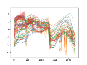
Figure 5: Training and test data for the hyper-spectral example

Similar to the previous example the largest wavelengths were noisy and were removed for this example. The length scale of this example was very short, as seen in Figure 5 and it was found to be computationally unfeasible to include sufficient numbers of inducting points in the wavelengths to capture the features of this dataset so the wavelengths were each treated as independent, although it would be preferable to include the covariance over wavelengths. In this 16 inducing points and 2 latent variables.

E.5 Oil Flow Classification

This example had uncorrelated input locations, with 10 latent dimensions and 16 inducing points.

References

• Ahmed et al. (2019) Ahmed, S., Rattray, M., and Boukouvalas, A. GrandPrix: Scaling up the Bayesian GPLVM for single-cell data. Bioinformatics, 35(1):47–54, 2019.
• Ajirak et al. (2022) Ajirak, M., Liu, Y., and Djurić, P. M. Ensembles of Gaussian process latent variable models. In 2022 30th European Signal Processing Conference (EUSIPCO), pp.  1467–1471. IEEE, 2022.
• Alsmeyer et al. (2004) Alsmeyer, F., Koß, H.-J., and Marquardt, W. Indirect spectral hard modeling for the analysis of reactive and interacting mixtures. Applied spectroscopy, 58(8):975–985, 2004.
• Altmann et al. (2013) Altmann, Y., Dobigeon, N., McLaughlin, S., and Tourneret, J.-Y. Nonlinear spectral unmixing of hyperspectral images using Gaussian processes. IEEE Transactions on Signal Processing, 61(10):2442–2453, 2013. doi: 10.1109/TSP.2013.2245127.
• Baldridge et al. (2009) Baldridge, A. M., Hook, S. J., Grove, C., and Rivera, G. The ASTER spectral library version 2.0. Remote sensing of environment, 113(4):711–715, 2009.
• Barker & Rayens (2003) Barker, M. and Rayens, W. Partial least squares for discrimination. Journal of Chemometrics: A Journal of the Chemometrics Society, 17(3):166–173, 2003.
• Barnes et al. (1989) Barnes, R., Dhanoa, M. S., and Lister, S. J. Standard normal variate transformation and de-trending of near-infrared diffuse reflectance spectra. Applied spectroscopy, 43(5):772–777, 1989.
• Bishop & James (1993) Bishop, C. M. and James, G. D. Analysis of multiphase flows using dual-energy gamma densitometry and neural networks. Nuclear Instruments and Methods in Physics Research Section A: Accelerators, Spectrometers, Detectors and Associated Equipment, 327(2-3):580–593, 1993.
• Borsoi et al. (2019) Borsoi, R. A., Imbiriba, T., and Bermudez, J. C. M. Deep generative endmember modeling: An application to unsupervised spectral unmixing. IEEE Transactions on Computational Imaging, 6:374–384, 2019.
• Borsoi et al. (2021) Borsoi, R. A., Imbiriba, T., Bermudez, J. C. M., Richard, C., Chanussot, J., Drumetz, L., Tourneret, J.-Y., Zare, A., and Jutten, C. Spectral variability in hyperspectral data unmixing: A comprehensive review. IEEE geoscience and remote sensing magazine, 9(4):223–270, 2021.
• Chatterjee et al. (2021) Chatterjee, M., Le Roux, J., Ahuja, N., and Cherian, A. Visual scene graphs for audio source separation. In Proceedings of the IEEE/CVF International Conference on Computer Vision (ICCV), pp.  1204–1213, 2021.
• Dai et al. (2017) Dai, Z., Álvarez, M., and Lawrence, N. Efficient modeling of latent information in supervised learning using Gaussian processes. Advances in Neural Information Processing Systems, 30, 2017.
• Damianou et al. (2016) Damianou, A. C., Titsias, M. K., and Lawrence, N. D. Variational inference for latent variables and uncertain inputs in Gaussian processes. Journal of Machine Learning Research, 17(42):1–62, 2016.
• Dau et al. (2019) Dau, H. A., Bagnall, A., Kamgar, K., Yeh, C.-C. M., Zhu, Y., Gharghabi, S., Ratanamahatana, C. A., and Keogh, E. The UCR time series archive. IEEE/CAA Journal of Automatica Sinica, 6(6):1293–1305, 2019.
• de Souza et al. (2021) de Souza, D., Mesquita, D., Gomes, J. P., and Mattos, C. L. Learning GPLVM with arbitrary kernels using the unscented transformation. In International Conference on Artificial Intelligence and Statistics, pp.  451–459. PMLR, 2021.
• Dirks & Poole (2019) Dirks, M. and Poole, D. Incorporating domain knowledge about xrf spectra into neural networks. In Workshop on Perception as Generative Reasoning, NeurIPS, 2019.
• Gardner et al. (2018) Gardner, J., Pleiss, G., Weinberger, K. Q., Bindel, D., and Wilson, A. G. Gpytorch: Blackbox matrix-matrix gaussian process inference with gpu acceleration. Advances in neural information processing systems, 31, 2018.
• Gerretzen et al. (2015) Gerretzen, J., Szymańska, E., Jansen, J. J., Bart, J., van Manen, H.-J., van den Heuvel, E. R., and Buydens, L. M. Simple and effective way for data preprocessing selection based on design of experiments. Analytical chemistry, 87(24):12096–12103, 2015.
• He et al. (2022) He, P., Emami, P., Ranka, S., and Rangarajan, A. Self-supervised robust scene flow estimation via the alignment of probability density functions. In Proceedings of the AAAI Conference on Artificial Intelligence, volume 36, pp.  861–869, 2022.
• Hong et al. (2021) Hong, D., Gao, L., Yao, J., Yokoya, N., Chanussot, J., Heiden, U., and Zhang, B. Endmember-guided unmixing network (EGU-Net): A general deep learning framework for self-supervised hyperspectral unmixing. IEEE Transactions on Neural Networks and Learning Systems, 33(11):6518–6531, 2021.
• Jayaram & Thickstun (2020) Jayaram, V. and Thickstun, J. Source separation with deep generative priors. In International Conference on Machine Learning, pp.  4724–4735. PMLR, 2020.
• Jørgensen & Hauberg (2021) Jørgensen, M. and Hauberg, S. Isometric Gaussian process latent variable model for dissimilarity data. In International Conference on Machine Learning, pp.  5127–5136. PMLR, 2021.
• Kappatou et al. (2023) Kappatou, C. D., Odgers, J., García-Muñoz, S., and Misener, R. An optimization approach coupling preprocessing with model regression for enhanced chemometrics. Industrial & Engineering Chemistry Research, 62(15):6196–6213, 2023.
• Kazlauskaite et al. (2019) Kazlauskaite, I., Ek, C. H., and Campbell, N. Gaussian process latent variable alignment learning. In The 22nd International Conference on Artificial Intelligence and Statistics, pp.  748–757. PMLR, 2019.
• Kriesten et al. (2008) Kriesten, E., Alsmeyer, F., Bardow, A., and Marquardt, W. Fully automated indirect hard modeling of mixture spectra. Chemometrics and Intelligent Laboratory Systems, 91(2):181–193, 2008.
• Lalchand et al. (2022) Lalchand, V., Ravuri, A., and Lawrence, N. D. Generalised gplvm with stochastic variational inference. In International Conference on Artificial Intelligence and Statistics, pp.  7841–7864. PMLR, 2022.
• Lawrence & Hyvärinen (2005) Lawrence, N. and Hyvärinen, A. Probabilistic non-linear principal component analysis with Gaussian process latent variable models. Journal of machine learning research, 6(11), 2005.
• Manole & Ho (2022) Manole, T. and Ho, N. Refined convergence rates for maximum likelihood estimation under finite mixture models. In International Conference on Machine Learning, pp.  14979–15006. PMLR, 2022.
• Muñoz & Torres (2020) Muñoz, S. G. and Torres, E. H. Supervised extended iterative optimization technology for estimation of powder compositions in pharmaceutical applications: method and lifecycle management. Industrial & Engineering Chemistry Research, 59(21):10072–10081, 2020.
• Murphy (2022) Murphy, K. P. Probabilistic Machine Learning: An introduction, chapter 3.5. MIT Press, 2022. URL probml.ai.
• Neri et al. (2021) Neri, J., Badeau, R., and Depalle, P. Unsupervised blind source separation with variational auto-encoders. In 2021 29th European Signal Processing Conference (EUSIPCO), pp.  311–315. IEEE, 2021.
• Odgers et al. (2023) Odgers, J., Kappatou, C., Misener, R., García Muñoz, S., and Filippi, S. Probabilistic predictions for partial least squares using bootstrap. AIChE Journal, pp.  e18071, 2023.
• Paszke et al. (2019) Paszke, A., Gross, S., Massa, F., Lerer, A., Bradbury, J., Chanan, G., Killeen, T., Lin, Z., Gimelshein, N., Antiga, L., et al. Pytorch: An imperative style, high-performance deep learning library. Advances in neural information processing systems, 32, 2019.
• Pedregosa et al. (2011) Pedregosa, F., Varoquaux, G., Gramfort, A., Michel, V., Thirion, B., Grisel, O., Blondel, M., Prettenhofer, P., Weiss, R., Dubourg, V., et al. Scikit-learn: Machine learning in python. the Journal of machine Learning research, 12:2825–2830, 2011.
• Rakthanmanon et al. (2013) Rakthanmanon, T., Campana, B., Mueen, A., Batista, G., Westover, B., Zhu, Q., Zakaria, J., and Keogh, E. Addressing big data time series: Mining trillions of time series subsequences under dynamic time warping. ACM Transactions on Knowledge Discovery from Data (TKDD), 7(3):1–31, 2013.
• Ramchandran et al. (2021) Ramchandran, S., Koskinen, M., and Lähdesmäki, H. Latent Gaussian process with composite likelihoods and numerical quadrature. In International Conference on Artificial Intelligence and Statistics, pp.  3718–3726. PMLR, 2021.
• Rato & Reis (2019) Rato, T. J. and Reis, M. S. SS-DAC: A systematic framework for selecting the best modeling approach and pre-processing for spectroscopic data. Computers & Chemical Engineering, 128:437–449, 2019.
• Ritchie et al. (2020) Ritchie, A., Vandermeulen, R. A., and Scott, C. Consistent estimation of identifiable nonparametric mixture models from grouped observations. Advances in Neural Information Processing Systems, 33:11676–11686, 2020.
• Sharma & Chopra (2020) Sharma, R. and Chopra, K. EEG-based epileptic seizure detection using GPLV model and multi support vector machine. Journal of Information and Optimization Sciences, 41(1):143–161, 2020.
• Tauler (1995) Tauler, R. Multivariate curve resolution applied to second order data. Chemometrics and intelligent laboratory systems, 30(1):133–146, 1995.
• Titsias (2009) Titsias, M. Variational learning of inducing variables in sparse Gaussian processes. In Artificial intelligence and statistics, pp.  567–574. PMLR, 2009.
• Titsias & Lawrence (2010) Titsias, M. and Lawrence, N. D. Bayesian Gaussian process latent variable model. In Proceedings of the thirteenth international conference on artificial intelligence and statistics, pp.  844–851. JMLR Workshop and Conference Proceedings, 2010.
• Urtasun & Darrell (2007) Urtasun, R. and Darrell, T. Discriminative Gaussian process latent variable model for classification. In Proceedings of the 24th international conference on Machine learning, pp.  927–934, 2007.
• Williams & Rasmussen (2006) Williams, C. K. and Rasmussen, C. E. Gaussian processes for machine learning, volume 2. MIT press Cambridge, MA, 2006.
• Wold et al. (2001) Wold, S., Sjöström, M., and Eriksson, L. PLS-regression: a basic tool of chemometrics. Chemometrics and intelligent laboratory systems, 58(2):109–130, 2001.
• Wülfert et al. (1998) Wülfert, F., Kok, W. T., and Smilde, A. K. Influence of temperature on vibrational spectra and consequences for the predictive ability of multivariate models. Analytical chemistry, 70(9):1761–1767, 1998.
• Wytock & Kolter (2014) Wytock, M. and Kolter, J. Contextually supervised source separation with application to energy disaggregation. In Proceedings of the AAAI Conference on Artificial Intelligence, volume 28, 2014.
• Yip et al. (2022) Yip, K. H., Waldmann, I. P., Changeat, Q., Morvan, M., Al-Refaie, A. F., Edwards, B., Nikolaou, N., Tsiaras, A., de Oliveira, C. A., Lagage, P.-O., et al. ESA-Ariel data challenge NeurIPS 2022: Inferring physical properties of exoplanets from next-generation telescopes. arXiv preprint arXiv:2206.14642, 2022.