Theory of biexciton-polaritons in transition metal dichalcogenide monolayers

Abstract

We theoretically investigate a nonlinear optical response of a planar microcavity with an embedded transition metal dicalcogenide monolayer of a when an energy of a biexcitonic transition is brought in resonance with an energy of a cavity mode. We demonstrate that the emission spectrum of this system strongly depends on an external pump. For small and moderate pumps we reveal the presence of a doublet in the emission with the corresponding Rabi splitting scaling as a square root of the number of the excitations in the system. Further increase of the pump leads to the reshaping of the spectrum, which demonstrates the pattern typical for a Mollow triplet. An intermediate pumping regime shows a broad irregular spectrum reminiscent of a chaotic dynamics of the system.

Introduction.—Transitional metal dichalcogenides (TMDs) is a novel class of truly two-dimensional (2D) materials with fascinating optical response, dominated by bound electron-hole complexes, formed due to the strong Coulomb attraction between photocreated carriers. The simplest example of such a complex is an exciton, a bound state of an electron-hole pair, representing a solid state analogue of a hydrogen atom [1, 2, 3, 4, 5, 6, 7, 8]. The unique combination of the properties characteristic of TMD materials, including specific 2D screening [9, 10], relatively large reduced mass of an electron-hole pair [11, 12, 13], nontrivial valley dynamics [14, 15, 16], and high binding energies making bright excitons stable even at room temperatures [4, 17, 18] distinguishes them from conventional semiconductors. Moreover, because of the large binding energy and small Bohr radius of the excitons, their coupling to light is dramatically increased [19, 20, 21, 18]. Therefore, if a TMD monolayer (ML) is placed inside a photonic cavity, one can relatively easily reach the regime of the strong light-matter coupling, where exciton-polaritons, hybrid half-light, half matter elementary excitations, emerge [16, 22, 23, 24, 25].

However, excitons are not the only type of the bound electron-hole complexes that can be formed. In doped samples, where photocreated excitons interact with a Fermi sea of resident charge carriers, electrons or holes, formation of trions and Fermi polarons [26, 27] becomes possible. Similar to the case of excitons, strong light-matter coupling can be routinely achieved for trions/Fermi-polarons resulting in a plethora of mixed light-matter quasi-particles [28, 29, 30, 31, 32, 33, 34, 35, 36, 37, 38, 39, 40, 41, 42, 43].

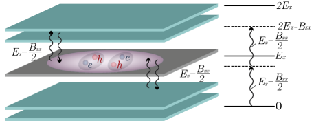
Figure 1: Schematic presentation of the analyzed system and related processes. A monolayer of WS₂ is placed between two dielectric Bragg mirrors (DBRs) in an antinode of a confined photonic cavity mode. The cavity mode is resonantly tuned to biexcitonic resonance, so that the photon energy $E_{c}$ is twice smaller than that of a biexciton $E_{b}=2E_{x}-B_{xx}$, where $E_{x}$ is the exciton energy and $B_{xx}$ is the binding energy of a biexciton. Creation of a biexciton is a two photon process, which makes the behavior of the system strongly dependent on the pump intensity.

Besides attaching a free electron, two excitons in a TMD ML can bind together, forming a biexciton, a solid state analog of a hydrogen molecule [44, 45, 46, 47, 48, 49, 50, 51, 52, 53, 54, 55]. The characteristic binding energies can reach 50 meV [44, 45], which is more than an order of magnitude higher compared to conventional semiconductor quantum wells, and makes biexcitons in TMD MLs stable up to room temperature. These excitonic molecules underlie basic nonlinear response of 2D semiconductors, reveal intriguing many-body physics and can serve in particular as a platform for quantum optics experiments due to their cascaded emission accompanied by entangled photon generation [56, 57, 58].

Although formation of biexcitons in TMD MLs is well studied both experimentally [44, 45, 46, 47, 48, 49, 50, 51, 52, 53, 54, 55] and theoretically [59, 60, 61, 62, 63, 64, 65, 66, 67], formation of biexciton-based composite half-light half-matter particles did not attract a due attention, to the best of our knowledge. The possibility of a formation of a bipolariton resonance in conventional semiconductor-quantum-well-based planar microcavities was predicted years ago [68, 69] and later on experimentally confirmed [70], but a detailed analysis of the biexciton-photon coupling in TMD materials, in particular, the emerging emission pattern in the regime of strong matter coupling and its microscopic characteristics, is still lacking. In this Letter, we propose a corresponding microscopic theory.

Model. — We consider the system schematically shown in Fig. 1. A monolayer of a TMD material is placed inside a planar microcavity. The confined photonic modes of two opposite circular polarizations are resonantly coupled with excitons in TMD ML. For simplicity, we consider the case corresponding to in-plane momentum $\textbf{k}=0$.

Let $c_{\sigma}^{\dagger}$ and $c_{\sigma}$ be the creation and annihilation operators of the cavity mode, $x_{\sigma}^{\dagger}$ and $x_{\sigma}$ be the corresponding excitonic operators, and $b^{\dagger}$ and $b$ those of a bright biexciton (which is a singlet both in two electron and two hole spins/valleys) with $\sigma=\pm$ denoting the corresponding circular polarization. We treat excitons and biexcitons as ideal bosons, neglecting the nonlinear effects stemming from their composite statistics [71]. The corersponding model Hamiltonian reads:

$$\mathcal{H}=\sum_{\sigma=\pm}E_{c}c_{\sigma}^{\dagger}c_{\sigma}+\sum_{\sigma=\pm}E_{x}x_{\sigma}^{\dagger}x_{\sigma}+E_{b}b^{\dagger}b+\\ +\sum_{\sigma=\pm}V_{x}(c_{\sigma}^{\dagger}x_{\sigma}+x_{\sigma}^{\dagger}c_{\sigma})+\\ +V_{b}(c_{+}^{\dagger}x_{-}^{\dagger}b+b^{\dagger}x_{-}c_{+}+c_{-}^{\dagger}x_{+}^{\dagger}b+b^{\dagger}x_{+}c_{-}).$$ (1)

We assumed that the main process of the biexciton formation is the cascade process of $c\to x\to b$. The process of the direct two-photon absorption and creation of biexciton via remote states is weaker and can be analyzed separately [72]. We assume that the differences $E_{c}-E_{x}$ and $E_{b}-2E_{x}$ are by far smaller than the energies of other states making it possible to keep only the processes described by the Halimitonian (1). We also consider the case of an undoped microcavity, and so neglect the possibility of the formation of trions and exciton polarons.

It is important to note that the combination of strong spin-orbit interaction and violation of the inversion symmetry of the system leads to additional valley degrees of freedom. The valley structure leads to the fact that the optical transition being direct is sensitive to the choice of light polarization and can only be induced in the so-called $K_{+}$ or $K_{-}$ valleys.

The parameters $V_{x}$ and $V_{b}$ are the matrix elements of the photon-exciton and exciton-biexciton conversion. To determine them we recall that the light-matter interaction in the basis of electrons and holes can be described by the following Hamiltonian

$$H_{\textup{l-m}}=\sum_{\bm{k},\sigma=\pm}\Omega(a^{\dagger}_{e,\bm{k},\sigma}a^{\dagger}_{h,-\bm{k},\sigma}c_{\sigma}+{\rm h.c.}),$$ (2)

where the constant $\Omega$ is proportional to the electric field in the mode and interband dipole matrix element, $a^{{\dagger}}_{e,\bm{k},\sigma}$, $a^{\dagger}_{h,\bm{k},\sigma}$ are the electron and hole creation operators (correspondingly, $a_{e,\sigma k}$, $a_{h,\sigma k}$ are the electron and hole annihilation operators). Note also that for charge carriers $+$ and $-$ denote spin components (or valley indices) and we assume that the optical transition selection rules correspond to the simplest case $\sigma=+\quad\Rightarrow\quad(e+,h+);\quad\sigma=-\quad\Rightarrow\quad(e-,h-).$ In Eq. (2) we neglected the wave vector of light so that the momenta of the photoexcited electron and hole are opposite.

The exciton state can be represented as:

$$\Psi_{x,\sigma}=\sum_{\bm{k}_{e},\bm{k}_{h}}F({\bf k}_{e},{\bf k}_{h})a^{\dagger}_{e,{\bf k}_{e},\sigma}a^{\dagger}_{h,{\bf k}_{h},\sigma}|0\rangle,$$ (3)

where $|0\rangle$ is the ground state of the system with empty conduction band and filled valence band and $F(\bm{k}_{e},{\bf k}_{h})$ is the Fourier transform of a two-particle envelope function,

$$F({\bf k}_{e},{\bf k}_{h})=\dfrac{1}{S}\int{\rm d}{\bf r}_{e}{\rm d}{\bf r}_{h}\psi_{{\bf K}_{\textup{ex}}}({\bf r}_{e},{\bf r}_{h})e^{-\mathrm{i}{\bf k}_{e}{\bf r}_{e}-\mathrm{i}{\bf k}_{h}{\bf r}_{h}},$$ (4)

where $S$ is a quantization area of the sample. In this paper, we restrict ourselves to consideration of a biexciton consisting of excitons with a zero wave vector. In this case, $\bm{K}_{\textup{ex}}\equiv\bm{k}_{e}+\bm{k}_{h}=0$ and $F({\bf k}_{e},{\bf k}_{h})\propto\delta_{{\bf k}_{e},-{\bf k}_{h}}$. Combining Eqs. (2) and (3), we obtain:

$$V_{x}=\langle\Psi_{x,\sigma}|H_{\textup{l-m}}c_{\sigma}^{\dagger}|0\rangle=\Omega\sum_{\bf k}F^{*}({\bf k},-{\bf k})=\\ =\Omega\int{\rm d}{\bf r}\psi_{{\bf K}_{\textup{ex}}=0}^{*}({\bf r},{\bf r})=\sqrt{S}\Omega\varphi_{x}^{*}(0),$$ (5)

where $\varphi_{x}(\rho)$ is the envelope function of the relative motion of the electron and hole in the exciton

$$\psi_{{\bf K}_{\textup{ex}}}({\bf r}_{e},{\bf r}_{h})=\dfrac{1}{\sqrt{S}}\,\varphi_{x}(|{\bf r}_{e}-{\bf r}_{h}|)e^{\mathrm{i}{\bf K}_{\textup{ex}}{\bf R}},$$ (6)

where ${\bf R}=(m_{e}{\bf}r_{e}+m_{h}{\bf}r_{h})/M$, and the total mass of the exciton is defined as $M=m_{e}+m_{h}$. The parameter $V_{b}$ can be evaluated in a similar way. Representing the biexciton wave function as

$$\Psi_{b}=\sum\limits_{\begin{subarray}{c}\bm{k}_{e},\bm{k}_{h}\\ \bm{k}_{e}^{\prime},\bm{k}_{h}^{\prime}\end{subarray}}B({\bf k}_{e},{\bf k}_{e}^{\prime},{\bf k}_{h},{\bf k}_{h}^{\prime})\frac{a^{\dagger}_{e,\bm{k}_{e},+}a^{\dagger}_{e,\bm{k}_{e}^{\prime},-}-a^{\dagger}_{e,\bm{k}_{e},-}a^{\dagger}_{e,\bm{k}_{e}^{\prime},+}}{\sqrt{2}}\frac{a^{\dagger}_{h,\bm{k}_{h},+}a^{\dagger}_{h,\bm{k}_{h}^{\prime},-}-a^{\dagger}_{h,\bm{k}_{h},-}a^{\dagger}_{h,\bm{k}_{h}^{\prime},+}}{\sqrt{2}}|0\rangle,$$ (7)

$$B({\bf k}_{e},{\bf k}_{e}^{\prime},{\bf k}_{h},{\bf k}_{h}^{\prime})=\dfrac{1}{S^{2}}\int{\rm d}{\bf r}_{e}{\rm d}{\bf r}_{h}{\rm d}{\bf r}_{e}^{\prime}{\rm d}{\bf r}_{h}^{\prime}\psi_{b}({\bf r}_{e},{\bf r}_{e}^{\prime},{\bf r}_{h},{\bf r}_{h}^{\prime})e^{-\mathrm{i}{\bf k}_{e}{\bf r}_{e}-\mathrm{i}{\bf k}_{h}{\bf r}_{h}-\mathrm{i}{\bf k}_{e}^{\prime}{\bf r}_{e}^{\prime}-\mathrm{i}{\bf k}_{h}^{\prime}{\bf r}_{h}^{\prime}},$$ (8)

where we have explicitly antisymmetrized the two-electron and two-hole functions, we obtain

$$V_{b}=\Omega\!\int\!\!{\rm d}{\bf r}_{1}{\rm d}{\bf r}_{2}\varphi_{x}(|{\bf r}_{2}|)\psi({\bf r}_{1}-{\bf r}_{2},{\bf r}_{1},{\bf r}_{2}/2).$$ (9)

Here we made use of the fact that the biexciton envelope function $\psi_{b}$ can be represented as

$$\!\!\psi_{b}({\bf r}_{e},\!{\bf r}_{e}^{\prime},\!{\bf r}_{h},\!{\bf r}_{h}^{\prime})=\frac{1}{\sqrt{S}}\,\psi({\bf r},{\bf r}^{\prime},{\bf R})e^{i{\bf K}_{b}{\bf R}_{b}},$$ (10)

where $\bm{K}_{b}$ is the exciton translational motion wave vector, ${\bf r}={\bf r}^{\prime}_{e}-{\bf r}_{e}$, ${\bf r}^{\prime}={\bf r}^{\prime}_{h}-{\bf r}_{h}$, $R=({\bf r}_{e}+{\bf r}^{\prime}_{e}-{\bf r}_{h}-{\bf r}^{\prime}_{h})/2$, ${\bf R}_{b}=[m_{e}({\bf r}_{e}+{\bf r}^{\prime}_{e})+m_{h}({\bf r}_{h}+{\bf r}^{\prime}_{h})]/2M$.

The function $\psi$ in Eq. (10) can be found variationally extending the approach developed in Ref. [73] for TMD ML case where the Coulomb interaction is described by the Rytova-Keldysh potential [74, 75]. The trial function is chosen in the form

$$\psi({\bf r},{\bf r}^{\prime},{\bf R})=\dfrac{\left[(kv)^{\nu}\!\exp{\left(-\rho kv\right)}+\lambda\exp{\left(-\tau kv\right)}\right]}{\sqrt{N_{b}}}\\ \times\exp{\left[-\dfrac{k(s_{1}+s_{2})}{2}\right]}\cosh{\left[\dfrac{\beta k(t_{1}-t_{2})}{2}\right]},$$ (11)

where $s_{1}=r_{eh}+r_{eh^{\prime}}$, $t_{1}=r_{eh}-r_{eh^{\prime}}$, $s_{2}=r_{e^{\prime}h}+r_{e^{\prime}h^{\prime}}$, $t_{2}=r_{e^{\prime}h}-r_{e^{\prime}h^{\prime}}$, $u=r_{ee^{\prime}}$, $v=r_{hh^{\prime}}$, $r_{ij}\equiv|{\bf r}_{i}-{\bf r}_{j}|$, and $N_{b}$ is a normalization factor (see the Supplemental Materials for details). The variational parameters are the following: dimensional $k$ and dimensionless $\beta$, $\nu$, $\rho$, $\lambda$, and $\tau$. They are found by maximizing the total binding energy $B_{2e,2h}$ of the four-particle system. Using the trial function (11), we obtain for the exciton-biexciton conversion matrix element:

$$V_{b}=\alpha\frac{a_{\textup{B}}}{\sqrt{S}}V_{x},$$ (12)

where dimensionless parameter $\alpha$ reads:

$$\alpha=\dfrac{2\pi}{\tilde{k}\sqrt{\tilde{N}_{b}}}\int\limits_{0}^{\infty}x{\rm d}x\int\limits_{0}^{\infty}y{\rm d}y\int\limits_{0}^{2\pi}{\rm d}\theta\ \phi{\left(y/\tilde{k}\right)}\\ \times\exp{\left(-\dfrac{x+y+\sqrt{x^{2}+y^{2}-2xy\cos{\theta}}}{2}\right)}\\ \times\cosh{\left[\dfrac{\beta\left(y-x-\sqrt{x^{2}+y^{2}-2xy\cos{\theta}}\right)}{2}\right]}\\ \times\left[x^{\nu}\exp{\left(-\rho x\right)}+\lambda\exp{\left(-\tau x\right)}\right].$$ (13)

Here we have introduced dimensionless parameter $\tilde{k}=a_{\textup{B}}k$ and normalization factor $\tilde{N}_{b}=a_{\textup{B}}N_{b}$, where $a_{\textup{B}}$ is the Bohr radius.

The Hamiltonian (1) allows us to formulate the set of the equations of motion for the system. We first write the Heisenberg equations of motion for the operators $c_{\pm},x_{\pm},b$ and then use the mean-filed approximation, replacing the secondary quantization operators by corresponding classical fields, $c_{\pm}\rightarrow C_{\pm}=\langle c_{\pm}\rangle$, and corresponding amplitudes $x_{\pm}\rightarrow X_{\pm}=\langle x_{\pm}\rangle$ and $b\rightarrow B=\langle b\rangle$ where the angle brackets $\langle\ldots\rangle$ denote a quantum mechanical averages. The resulting system reads [cf. Ref. [76], Eqs. (7.11)-(7.13)]

$$\mathrm{i}\hbar\frac{{\rm d}C_{\pm}}{{\rm d}t}= E_{c}C_{\pm}+V_{x}X_{\pm}+V_{b}X_{\mp}^{*}B,$$ (14a)

$$\mathrm{i}\hbar\frac{{\rm d}X_{\pm}}{{\rm d}t}= E_{x}X_{\pm}+V_{x}C_{\pm}+V_{b}C_{\mp}^{*}B,$$ (14b)

$$\mathrm{i}\hbar\frac{{\rm d}B}{{\rm d}t}= E_{b}B+V_{b}(X_{-}C_{+}+X_{+}C_{-}).$$ (14c)

We focus on the transient response of the microcavity after a short optical pump pulse that creates non-zero photonic occupancy $C_{\pm}(t=0)\neq 0$, analyzing the dynamics in real time and get the corresponding energy spectrum via its Fourier transform.

Results and discussion. — In this paper we consider the case of a WS₂ ML placed in a microcavity (the cases of the other TMD materials can be analyzed similarly). We use the following set of material parameters: the band gap $E_{g}=2.238$ eV [77], effective dielectric constant $\varepsilon$ and screening radius $r_{0}$ in the Rytova-Keldysh potential are chosen to be $4.4$ and $0.89~{}\textup{nm}$, respectively [77, 78, 79, 9]. The effective masses of the carriers are $m_{e}=0.26m_{0}$ and $m_{h}=0.35$ [78], which leads to the electron-hole reduced mass $\mu=m_{e}m_{h}/M=0.149m_{0}$ and electron-hole mass ratio $\sigma=m_{e}/m_{h}=0.743$. By numerically solving the Schrödinger equation for selected values of the parameters, we found the following value of the exciton binding energy: $B_{x}=152~{}\textup{meV}$. Thus, the energy of the exciton transition is $E_{x}=E_{g}-B_{x}=2.086~{}\textup{eV}$ that roughly corresponds to the experimental data [80].

For the light-matter coupling constant $\Omega$ determining $V_{x}$ via Eq. (5), we use the standard expression for the $\lambda/2$ cavity (we use SI units) [81]: $\Omega=\sqrt{E_{c}/2\varepsilon\varepsilon_{0}V}d_{\textup{cv}}$, where $V=LS$ is the cavity volume, $L=\pi c\hbar/E_{c}$ is the effective cavity length, and $d_{\rm cv}$ is the interband dipole matrix element. The latter is expressed within the $\mathbf{k}\mathbf{p}$-model as $d_{\textup{cv}}=e\hbar v_{F}/E_{g}$, where the ‘interband’ velocity $v_{F}$ for WS₂ amounts to $6.65\times 10^{5}$ m/s [82, 83].

Finally, we present the exciton envelope function at coinciding coordinates $\varphi_{x}(0)=\eta/a_{\textup{B}}$, where the Bohr radius is defined as $a_{\textup{B}}=4\pi\varepsilon_{0}\varepsilon\hbar^{2}/e^{2}\mu$ and the dimensionless parameter $\eta=0.615$ is extracted from the numerical ground-state solution of the excitonic Schrödinger equation. Taking into account all of the above, we obtain

$$V_{x}=\dfrac{\eta v_{F}e}{E_{g}a_{\textup{B}}}\sqrt{\dfrac{\hbar E_{c}^{2}}{2\pi c\varepsilon\varepsilon_{0}}}.$$ (15)

We assume that a biexciton is created resonantly, so that the biexciton energy is twice as large as the photon energy, $E_{b}=2E_{c}$. Using the set of the parameters specified above, we get $V_{x}=9.11~{}\textup{meV}$ ($E_{c}=2.0815$ eV).

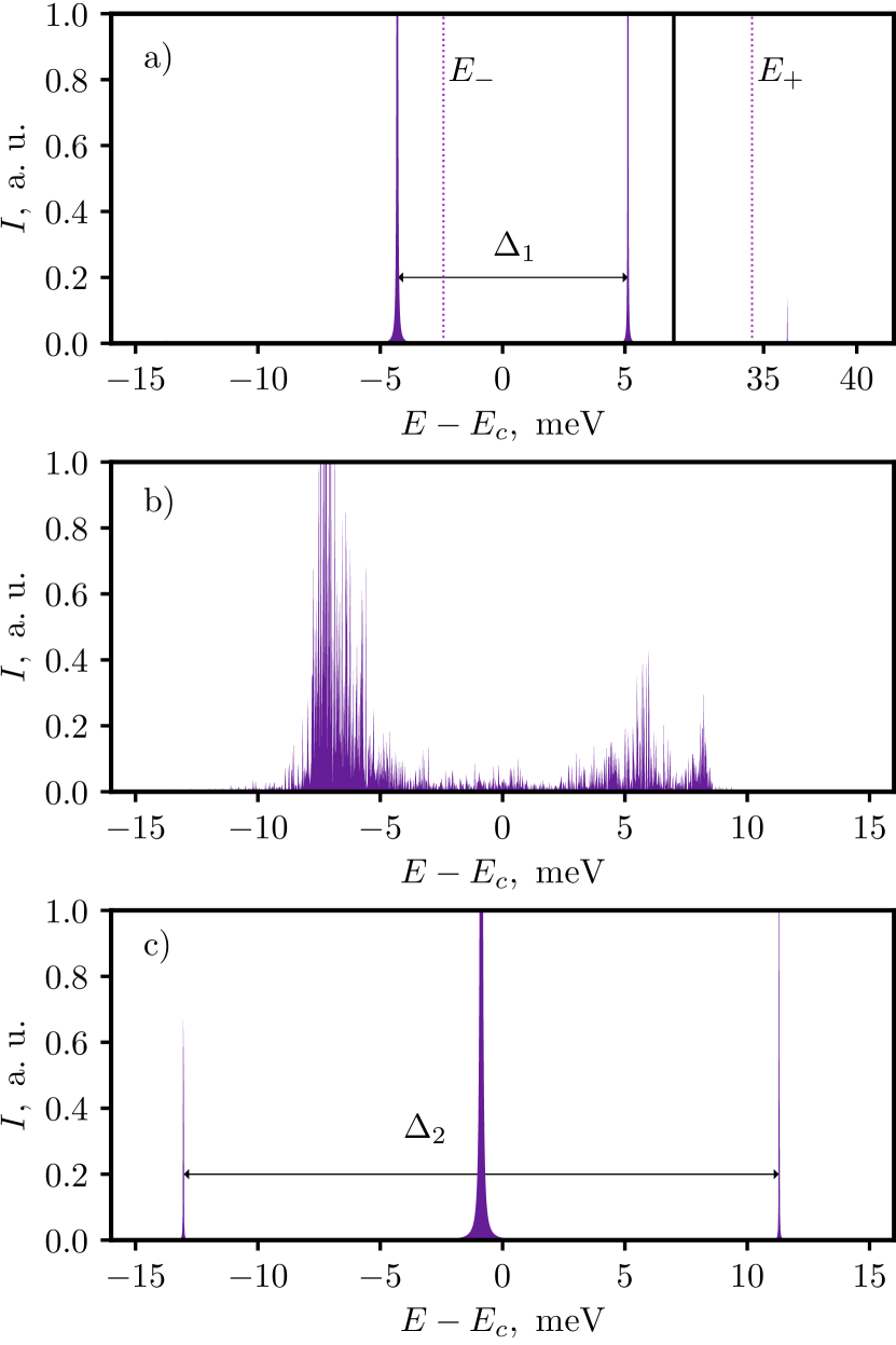
Figure 2: The emission spectra of the system for various values of pumping magnitude characterized by total number of the excitations $N$. The upper panel a) corresponds to relatively weak pumps, where two main peaks resembling Rabi-like splitting, together with a third weak peak in the high energy region are observed. The center panel b) illustrates a transient regime of intermediate pumps without regular structure of the peaks, characteristic to the chaotization of the nonlinear dynamics of the system. The lower panel c) demonstrates the formation of clear Mollow-type triplet pattern which is observed for high pumps.

Maximization of the biexcitonic binding energy with variational biexcitonic wavefunction 11 allows to determine the parameter $\alpha=1.01556$, corresponding to the biexciton to light coupling constant $V_{b}$ (see Eq.12).

Note, that differently form $V_{x}$, $V_{b}$ explicitly depends on the sample area $S$. To get rid of this dependence, which should not influence the systems dynamics, one can pass in Eqs. (14) to the normalized amplitudes, $C_{\pm}\rightarrow\tilde{C}_{\pm}\sqrt{\tilde{S}}$, and then solve numerically the resulting system which do not contain $S$ any more.

To get the emission spectrum, one needs to calculate a Fourier transform:

$$I(E)=\left|\int\limits_{0}^{\infty}\tilde{C}(t)e^{\mathrm{i}Et}dt\right|^{2}.$$ (16)

The corresponding spectra are plotted in Fig. 2 for three different pumps, corresponding to the initial number of photons in a cavity $N$ defined as $\tilde{C}_{\pm}(\tilde{t}=0)=\sqrt{N}$, $\tilde{X}_{\pm}(\tilde{t}=0)=0$, and $\tilde{B}(t=0)=0$. The chosen three cases illustrate the key regimes characterizing biexciton-polariton formation: (a) small to moderate $N<N_{c,1}$ where $N_{c,1}\approx 1.9$ for our parameters, (b) intermediate $N_{c,1}<N<N_{c,2}$, and (c) large $N>N_{c,2}$.

In the regime (a), two main peaks resembling a Rabi doublet are seen in the spectrum (corresponding to $E-E_{c}\approx\pm 5$meV), together with an additional peak located slightly above 35 meV, see Fig.2a. These three peaks originate from the mixture of photonic, excitonic and biexcitonic modes. If one switches off the photon-biexciton coupling putting $\alpha=0$, the central peak disappears, and flanking peaks continously approach the positions of upper and lower exciton-polaritons, shown in the figure by vertical dashed lines. Note, that as the formation of a biexciton is a two-photon process, the distance between the two main peaks increases with the photon occupancy [72], as it is shown in Fig. 3.

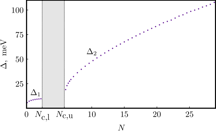
Figure 3: The splittings $\Delta_{1}$, characterizing the Rabi doublet regime (panel a at Fig.2), and $\Delta_{2}$, characterizing the Mollow triplet regime (panel b at Fig.2) as function of the pump intensity characterized by the number of the excitations $N$. The two regimes are separared by the gray vertical bar, corresponding to the chaotic regime characterized by broad multiple peaks structure

If the pump exceeds some critical value, the above described regular peak structure disappears, and the spectrum is characterized by a broad distribution of multiple peaks characteristic to the transition to chaotic dynamics of the system described by nonlinear set of equations 14c, see Fig. 3b.

Finally, for sufficiently high pumps the spectrum again becomes regular, but now the pattern closely resembling the Mollow triplet is formed, see Fig.2. The strong central peak is located around the position corresponding to the cavity photon, while the distance between the satellite peaks $\Delta_{2}$ between the outer peaks increases with increase of the pump, as it is shown in Fig. 3. This behavior is very similar to what is happening in the paragon case of Jaynes-Cummings model. However, differently from this latter case, Rabi doublet and Mollow triplet regimes are separated by the chaotic regime with broad spectral distribution, shown by the vertical gray bar in Fig. 3.

Conclusion.— We developed a microscopic theoretical approach for studying the emission spectrum of a quantum microcavity with an embedded TMD ML accounting for the resonant coupling of a cavity mode with both excitonic and biexcitonic transitions. As creation of a biexciton requires absorption of two photons with opposite circular polarizations, the formation of a biexciton-polariton is a strongly nonlinear process. We demonstrated that for weak pumps it is characterized by a Rabi-type doublet, while for large pumps radical reshaping of the emission spectrum takes place and the pattern resembling the Mollow triplet emerges. This two regimes are separated by the transitory regime characterized by broad multi-peak emission characteristic to chaotic dynamics of the system.