Generalized Double Affine Hecke Algebra for Double Torus

Abstract.

We propose a generalization of the double affine Hecke algebra of type-$C^{\vee}C_{1}$ at specific parameters by introducing a “Heegaard dual” of the Hecke operators. Shown is a relationship with the skein algebra on double torus. We give automorphisms of the algebra associated with the Dehn twists on the double torus.

1. Introduction

The double affine Hecke algebra (DAHA) was introduced by Cherednik for studies on the Knizhnik–Zamolodchikov equation and its applications to orthogonal symmetric polynomials via the Dunkl–Cherednik operators [8]. It is a fundamental modern tool in mathematics and physics. One of applications of DAHA is the skein algebra, which receives renewed interests from a viewpoint of the quantization of the character varieties. Although, the DAHA is so far only applicable for the skein algebra on the once-punctured torus $\Sigma_{1,1}$ and the 4-punctured sphere $\Sigma_{0,4}$. The former is the DAHA of type-$A_{1}$, and the latter is of type-$C^{\vee}C_{1}$ [24, 5, 16, 22]. The superpolynomials for links on $\Sigma_{1,1}$ and $\Sigma_{0,4}$ were constructed by use of the automorphism of DAHA [9, 10].

A generalization of DAHA for the skein algebra on higher-genus surface was initiated in [3, 2]. Constructed are $q$-difference operators for generators of the skein algebra on $\Sigma_{2,0}$ as a $\mathbb{Z}_{3}$ generalization of the DAHA of type-$A_{1}$. Though the Iwahori–Hecke algebraic structure seems to be missing, shown was that it is isomorphic to the skein algebra on $\Sigma_{2,0}$ [12].

Another representation of the skein algebra on $\Sigma_{2,0}$ was given in our previous paper [16]. Combining the DAHAs of type-$A_{1}$ and $C^{\vee}C_{1}$, we constructed the $q$-difference operators for generators of the skein algebra [3, 2]. Using the automorphisms of $A_{1}$ DAHA, we computed the DAHA polynomial for double twist knots, and observed a relationship with the colored Jones polynomials. The present paper relies on [16], but we rather aim to generalize the $C^{\vee}C_{1}$ DAHA at specific parameters by introducing “Heegaard dual” operators of $C^{\vee}C_{1}$ DAHA. Thus our generalization is different from [13] where the generalized DAHA was associated with a 2-dimensional crystallographic group.

This paper is organized as follows. In Section 2, we recall the skein algebra on surface and DAHA. We review an isomorphism between the skein algebra on the 4-punctured sphere and DAHA of type-$C^{\vee}C_{1}$. In Section 3, we pay attention to $C^{\vee}C_{1}$ DAHA at $\mathbf{t}_{\star}$. By introducing Heegaard dual operators, we propose a generalized DAHA. Using the automorphisms we study a relationship with the skein algebra on $\Sigma_{2,0}$.

Throughout this article we use

$$\operatorname{ch}(x)=x+x^{-1},\qquad\qquad\operatorname{sh}(x)=x-x^{-1}.$$ (1.1)

2. Preliminaries on DAHA of $C^{\vee}C_{1}$-type and Skein Algebra

2.1. DAHA of $C^{\vee}C_{1}$-type

We recall the double affine Hecke algebra ${H}_{q,\mathbf{t}}$ of type-$C^{\vee}C_{1}$ with 4 parameters $\mathbf{t}=(t_{0},t_{1},t_{2},t_{3})$ [23] (see also [8, 21]). The DAHA $H_{q,\mathbf{t}}$ is generated by $\mathsf{T}_{0}^{\pm 1}$, $\mathsf{T}_{1}^{\pm 1}$, $(\mathsf{T}^{\vee}_{0})^{\pm 1}$, and $(\mathsf{T}^{\vee}_{1})^{\pm 1}$ satisfying

$$\mathsf{T}_{0}+t_{0}-t_{0}^{-1}=\mathsf{T}_{0}^{-1}, \mathsf{T}_{1}+t_{1}-t_{1}^{-1}=\mathsf{T}_{1}^{-1},$$ (2.1)

$$\mathsf{T}^{\vee}_{0}+t_{2}-t_{2}^{-1}=\left(\mathsf{T}^{\vee}_{0}\right)^{-1}, \mathsf{T}^{\vee}_{1}+t_{3}-t_{3}^{-1}=\left(\mathsf{T}^{\vee}_{1}\right)^{-1},$$

and

$$\mathsf{T}_{1}^{\vee}\mathsf{T}_{1}\mathsf{T}_{0}\mathsf{T}_{0}^{\vee}=q^{-\frac{1}{2}}.$$ (2.2)

Here and hereafter we use

$$\mathsf{X}=\left(\mathsf{T}_{1}^{\vee}\mathsf{T}_{1}\right)^{-1}=q^{\frac{1}{2}}\mathsf{T}_{0}\mathsf{T}_{0}^{\vee},$$ (2.3)

$$\mathsf{Y}=\mathsf{T}_{1}\mathsf{T}_{0}.$$ (2.4)

The spherical DAHA is defined by

$$SH_{q,\mathbf{t}}=\mathsf{e}\,H_{q,\mathbf{t}}\,\mathsf{e},$$ (2.5)

where the idempotent $\mathsf{e}$ is

$$\mathsf{e}=\frac{1}{t_{1}+t_{1}^{-1}}\left(t_{1}+\mathsf{T}_{1}\right).$$ (2.6)

The polynomial representation is given as [23]

$$\mathsf{T}_{0} \mapsto{t_{0}}^{-1}\,\mathsf{s}\,\eth-\frac{q^{-1}\left({t_{0}}^{-1}-t_{0}\right)x^{2}+q^{-\frac{1}{2}}\left({t_{2}}^{-1}-t_{2}\right)x}{1-q^{-1}x^{2}}\,\left(1-\mathsf{s}\,\eth\right),$$ (2.7)

$$\mathsf{T}_{1} \mapsto{t_{1}}^{-1}\mathsf{s}+\frac{\left({t_{1}}^{-1}-t_{1}\right)+\left({t_{3}}^{-1}-t_{3}\right)x}{x^{2}-1}\,\left(\mathsf{s}-1\right),$$

$$\mathsf{T}_{0}^{\vee} \mapsto q^{-\frac{1}{2}}{\mathsf{T}_{0}}^{-1}x,$$

$$\mathsf{T}_{1}^{\vee} \mapsto x^{-1}{\mathsf{T}_{1}}^{-1}.$$

Here we mean

$$\left(\mathsf{s}\,f\right)(x)=f(x^{-1}),\qquad\qquad\qquad\left(\eth\,f\right)(x)=f(q\,x).$$ (2.8)

Then the idempotent (2.6) is a map to the symmetric Laurent polynomials, $\mathsf{e}:\mathbb{C}[x^{\pm 1}]\to\mathbb{C}[x+x^{-1}]$. The Askey–Wilson operator is given from (2.4) as

$$\left.\operatorname{ch}(\mathsf{Y})\right|_{\text{sym}}\mapsto W(x;\mathbf{t})\left(\eth-1\right)+W(x^{-1};\mathbf{t})\left(\eth^{-1}-1\right)+t_{0}t_{1}+\left(t_{0}\,t_{1}\right)^{-1},$$ (2.9)

where sym denotes an action on the symmetric Laurent polynomials, and

$$W(x;\mathbf{t})=t_{0}\,t_{1}\,\frac{\left(1-\frac{1}{t_{1}t_{3}}x\right)\left(1+\frac{t_{3}}{t_{1}}x\right)\left(1-q^{\frac{1}{2}}\frac{1}{t_{0}t_{2}}x\right)\left(1+q^{\frac{1}{2}}\frac{t_{2}}{t_{0}}x\right)}{\left(1-x^{2}\right)\left(1-q\,x^{2}\right)}.$$ (2.10)

The eigen-polynomial of (2.9) is the Askey–Wilson polynomial $P_{m}(x;q,\mathbf{t})$,

$$P_{m}(x;q,\mathbf{t})=\frac{(ab,ac,ad;q)_{m}}{a^{m}(abcdq^{m-1};q)_{m}}{}_{4}\phi_{3}\left[\begin{matrix}q^{-m},q^{m-1}abcd,ax,ax^{-1}\\ ab,ac,ad\end{matrix};q,q\right],$$ (2.11)

satisfying

$$\left(\mathsf{Y}+\mathsf{Y}^{-1}\right)P_{m}(x;q,\mathbf{t})=\operatorname{ch}\left(t_{0}t_{1}q^{-m}\right)\,P_{m}(x;q,\mathbf{t}),$$ (2.12)

where

$$a=\frac{1}{t_{1}t_{3}},\qquad b=-\frac{t_{3}}{t_{1}},\qquad c=\frac{q^{\frac{1}{2}}}{t_{0}t_{2}},\qquad d=-\frac{q^{\frac{1}{2}}t_{2}}{t_{0}}.$$

See [4, 15] for properties of the Askey–Wilson polynomials.

2.2. Skein Algebra on $\Sigma_{0,4}$

The skein algebra $\operatorname{Sk}_{A}(\Sigma)$ on surface $\Sigma$ is generated by isotopy classes of framed links in $\Sigma\times[0,1]$ satisfying the skein relation

$$\vbox{\hbox{ \leavevmode\hbox to38.45pt{\vbox to38.45pt{\text{[drawing]}}} }}=A\,\vbox{\hbox{ \leavevmode\hbox to29.65pt{\vbox to29.65pt{\text{[drawing]}}} }}+A^{-1}\,\vbox{\hbox{ \leavevmode\hbox to29.65pt{\vbox to29.65pt{\text{[drawing]}}} }},$$ (2.13)

$$\vbox{\hbox{ \leavevmode\hbox to29.65pt{\vbox to29.65pt{\text{[drawing]}}} }}=-A^{2}-A^{-2}.$$

A multiplication $\mathbb{x}\,\mathbb{y}$ of links $\mathbb{x}$ and $\mathbb{y}$ means that $\mathbb{x}$ is vertically above $\mathbb{y}$,

$$\mathbb{x}\,\mathbb{y}=\lx@add@Preamble@PI{\newcolumntype{C}{>{$}c<{$}}}\begin{tabular}[]{|C|}\hline\cr\hphantom{aa}\mathbb{x}\hphantom{aa}\\ \hline\cr\mathbb{y}\\ \hline\cr\end{tabular}$$

When two simple closed curves $\mathbb{x}$ and $\mathbb{y}$ on $\Sigma$ intersect exactly once, we have

$$\frac{1}{A^{\pm 2}-A^{\mp 2}}\left(A^{\pm 1}\mathbb{x}\,\mathbb{y}-A^{\mp 1}\mathbb{y}\,\mathbb{x}\right)=\mathscr{D}_{\mathbb{x}}^{\mp 1}(\mathbb{y}),$$ (2.14)

where $\mathscr{D}_{\mathbb{x}}$ denotes the left Dehn twist along $\mathbb{x}$. It is noted that

$$\mathscr{D}_{\mathbb{y}}(\mathbb{x})=\mathscr{D}_{\mathbb{x}}^{-1}(\mathbb{y}).$$ (2.15)

A finite set of Dehn twists along non-separating simple closed curves generates the mapping class group $\operatorname{Mod}(\Sigma_{g,0})$ of a surface $\Sigma_{g,0}$. See, e.g., [6, 14].

Figure 1. Simple closed curves on the 4-punctured sphere $\Sigma_{0,4}$.

In the case of the 4-punctured sphere $\Sigma_{0,4}$, the skein algebra is generated by $\mathbb{x}$, $\mathbb{y}$, and $\mathbb{b}_{i}$ in Fig. 1. It is known that the type-$C^{\vee}C_{1}$ DAHA is isomorphic to the skein algebra on the 4-punctured sphere [24, 16, 5]. See also [27, 19, 20, 25] from a point of view of the algebraic structure of the Askey–Wilson polynomials. The Askey–Wilson operator $\operatorname{ch}\mathsf{Y}$ and $\operatorname{ch}\mathsf{X}$ respectively corresponds to the curves $\mathbb{y}$ and $\mathbb{x}$, while the 4 parameters $(t_{0},t_{1},t_{2},t_{3})$ denote the boundary curves $(\mathbb{b}_{1},\mathbb{b}_{3},\mathbb{b}_{2},\mathbb{b}_{4})$. See [16] for detail. In addition, the generators of the $SL(2;\mathbb{Z})$ action [8] on $H_{q,\mathbf{t}}$

$$\sigma_{R}=\begin{pmatrix}1&1\\ 0&1\end{pmatrix} :\begin{pmatrix}\mathsf{T}_{0}\\ \mathsf{T}_{1}\\ \mathsf{X}\end{pmatrix}\mapsto\begin{pmatrix}q^{-\frac{1}{2}}\mathsf{X}\mathsf{T}_{0}^{-1}\\ \mathsf{T}_{1}\\ \mathsf{X}\end{pmatrix},$$ (2.16)

$$\sigma_{L}=\begin{pmatrix}1&0\\ 1&1\end{pmatrix} :\begin{pmatrix}\mathsf{T}_{0}\\ \mathsf{T}_{1}\\ \mathsf{X}\end{pmatrix}\mapsto\begin{pmatrix}\mathsf{T}_{0}\\ \mathsf{T}_{1}\\ q^{\frac{1}{2}}\mathsf{T}_{0}\mathsf{X}^{-1}\mathsf{T}_{1}^{-1}\end{pmatrix},$$ (2.17)

can be interpreted as the half Dehn twists along $\mathbb{x}$ and $\mathbb{y}$ respectively.

3. DAHA on Double Torus and Skein Algebra

3.1. Skein Algebra and Mapping Class Group on $\Sigma_{2,0}$

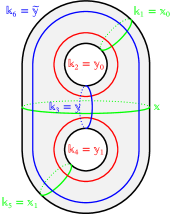
Figure 2. Simple closed curves on the double torus $\Sigma_{2,0}$.

The skein algebra $\operatorname{Sk}_{A}(\Sigma_{2,0})$ is generated by $\mathbb{k}_{1}=\mathbb{x}_{0}$, $\mathbb{k}_{2}=\mathbb{y}_{0}$, $\mathbb{k}_{3}=\mathbb{y}$, $\mathbb{k}_{4}=\mathbb{y}_{1}$, and $\mathbb{k}_{5}=\mathbb{x}_{1}$, where we label each simple closed curve on $\Sigma_{2,0}$ as in Fig. 2 following [16]. The Humphries generators of the mapping class group are $\mathscr{D}_{i}=\mathscr{D}_{\mathbb{k}_{i}}$ for $1\leq i\leq 5$, and the mapping class group is (see e.g. [6, 26])

$$\operatorname{Mod}(\Sigma_{2,0}) =\left\langle\mathscr{D}_{1},\dots,\mathscr{D}_{5}~{}\middle|~{}\begin{matrix}\text{$\mathscr{D}_{i,i+1,i}=\mathscr{D}_{i+1,i,i+1}$ for $1\leq i\leq 4$ }\\ \text{$\mathscr{D}_{i,j}=\mathscr{D}_{j,i}$ for $|i-j|>1$}\\ \left(\mathscr{D}_{1,2,3,4,5}\right)^{6}=1\\ \left(\mathscr{D}_{5,4,3,2,1,1,2,3,4,5}\right)^{2}=1\end{matrix}\right\rangle,$$ (3.1)

where we mean $\mathscr{D}_{i,\dots,j,k}=\mathscr{D}_{i}\dots\mathscr{D}_{j}\mathscr{D}_{k}$. We note that the 2- and 3-chain relations [14] respectively give

$$\left(\mathscr{D}_{1,2}\right)^{6}=\mathscr{D}_{\mathbb{x}},$$ (3.2)

$$\left(\mathscr{D}_{1,2,3}\right)^{4}=\mathscr{D}_{5}^{2}.$$ (3.3)

See Fig. 3 for several simple closed curves generated by the Dehn twists $\mathscr{D}_{i}$. We mean for simplicity $\mathbb{k}_{i,\pm j,\dots,\pm k}=\left(\mathscr{D}_{k}^{\pm 1}\dots\mathscr{D}_{j}^{\pm 1}\right)(\mathbb{k}_{i})$. These were used in [1] in studies of the character variety.

Figure 3. Several simple closed curves on $\Sigma_{2,0}$ generated by the Dehn twists $\mathscr{D}_{j}$ from $\mathbb{k}_{i}$.

3.2. $q$-Difference Operators

In [16] studied was the map

$$\mathcal{A}:\operatorname{Sk}_{A=q^{-\frac{1}{4}}}(\Sigma_{2,0})\to\operatorname{End}\mathbb{C}\left(q^{\frac{1}{4}},x_{0},x_{1}\right)\left[x+x^{-1}\right].$$ (3.4)

Therein given are for the curves in Fig. 2 as

$$\mathcal{A}(\mathbb{x}_{b})=\operatorname{ch}(x_{b}),$$ (3.5)

$$\mathcal{A}(\mathbb{y}_{b})=\mathrm{i}\,q^{-\frac{1}{4}}G_{0}(x_{b},x),$$ (3.6)

$$\mathcal{A}(\mathbb{x})=\operatorname{ch}(x),$$ (3.7)

$$\mathcal{A}(\mathbb{y})=\sum_{\epsilon=\pm}\omega(x^{\epsilon})\left\{-x^{-\epsilon}\left(x_{0}+\frac{q^{\frac{1}{2}}x^{\epsilon}}{x_{0}}\right)\left(x_{1}+\frac{q^{\frac{1}{2}}x^{\epsilon}}{x_{1}}\right)\,\eth^{\epsilon}+q^{\frac{1}{2}}\operatorname{ch}(x_{0})\operatorname{ch}(x_{1})\right\},$$ (3.8)

$$\mathcal{A}(\widetilde{\mathbb{y}})=\sum_{\epsilon=\pm}\omega(x^{\epsilon})\left\{K_{0}(x_{0},x^{\epsilon})\,K_{0}(x_{1},x^{\epsilon})\,\eth^{\epsilon}-G_{0}(x_{0},x)\,G_{0}(x_{1},x)\right\},$$ (3.9)

where $b=0,1$. Here we have used

$$\omega(x)=\frac{x\left(1+q^{\frac{1}{2}}x\right)}{q^{\frac{1}{2}}\left(1-x^{2}\right)\left(1-q^{\frac{1}{2}}x\right)},$$ (3.10)

and the $q$-difference operators $K_{n}(x_{b},x)$ and $G_{n}(x_{b},x)$ for $n\in\mathbb{Z}$ are defined by

$$K_{n}(x_{b},x) =\frac{-x_{b}^{-n}}{1-x_{b}^{2}}\,\eth_{b}+\frac{x_{b}^{n}\left(q^{\frac{1}{2}}x+x_{b}^{2}\right)\left(q^{\frac{3}{2}}x+x_{b}^{2}\right)}{q\,x\left(1-x_{b}^{2}\right)}\,\eth_{b}^{-1},$$ (3.11)

$$G_{n}(x_{b},x) =\frac{-x_{b}^{-n}}{1-x_{b}^{2}}\,\eth_{b}+\frac{x_{b}^{n}\left(q^{\frac{1}{2}}x+x_{b}^{2}\right)\left(q^{\frac{1}{2}}+x\,x_{b}^{2}\right)}{q^{\frac{1}{2}}\,x\left(1-x_{b}^{2}\right)}\,\eth_{b}^{-1},$$ (3.12)

where the $q$-shift operators $\eth_{b}$ for $b=0,1$ are

$$\left(\eth_{0}f\right)(x,x_{0},x_{1})=f(x,q^{\frac{1}{2}}x_{0},x_{1}),\qquad\qquad\left(\eth_{1}f\right)(x,x_{0},x_{1})=f(x,x_{0},q^{\frac{1}{2}}x_{1}).$$ (3.13)

Note that the $q$-difference operators $K_{0}(x_{b},x)$, $K_{0}(x_{b},x^{-1})$, and $G_{0}(x_{b},x)$ are respectively related to the raising operator, lowering operator, and the eigen-operator for the type-$A_{1}$ Macdonald polynomials a.k.a. the Rogers ultra-spherical polynomials [16]. We see that they fulfill the following;

$$G_{n}(x_{b},x^{-1})=G_{n}(x_{b},x),$$ (3.14)

$$K_{n}(x_{b},x)\,G_{n}(x_{b},q\,x)=G_{n}(x_{b},x)\,K_{n}(x_{b},x),$$ (3.15)

$$K_{n}(x_{b},x^{-1})\,K_{n}(x_{b},q^{-1}x)-\left[G_{n}(x_{b},x)\right]^{2}=-q^{\frac{n}{2}}x^{-1}\left(q^{\frac{1}{2}}-x\right)^{2},$$ (3.16)

$$\begin{multlined}q^{\frac{1}{2}}x\,(1-x^{2})\left(G_{n}(x_{b},x)\,G_{n}(x_{b},q^{-1}x)-K_{n}(x_{b},x)\,K_{n}(x_{b},x^{-1})\right)\\ +(1-q)\,x^{2}\left(K_{n}(x_{b},x)-K_{n}(x_{b},x^{-1})\right)G_{n}(x_{b},q^{-1}x)\\ =q^{\frac{n}{2}}\left(q^{\frac{1}{2}}-x\right)\left(1-q^{\frac{1}{2}}x\right)\left(1-x^{2}\right)\frac{q-x_{b}^{2}}{1-x_{b}^{2}},\end{multlined}q^{\frac{1}{2}}x\,(1-x^{2})\left(G_{n}(x_{b},x)\,G_{n}(x_{b},q^{-1}x)-K_{n}(x_{b},x)\,K_{n}(x_{b},x^{-1})\right)\\ +(1-q)\,x^{2}\left(K_{n}(x_{b},x)-K_{n}(x_{b},x^{-1})\right)G_{n}(x_{b},q^{-1}x)\\ =q^{\frac{n}{2}}\left(q^{\frac{1}{2}}-x\right)\left(1-q^{\frac{1}{2}}x\right)\left(1-x^{2}\right)\frac{q-x_{b}^{2}}{1-x_{b}^{2}},$$ (3.20)

$$\begin{pmatrix}K_{n+1}(x_{b},x^{-1})\\ G_{n+1}(x_{b},q^{-1}x)\end{pmatrix}=\frac{1}{x-q^{\frac{1}{2}}}\begin{pmatrix}x\operatorname{ch}(x_{b})&-\frac{q^{\frac{1}{2}}+x\,x_{b}^{2}}{x_{b}}\\ \frac{x+q^{\frac{1}{2}}x_{b}^{2}}{x_{b}}&-q^{\frac{1}{2}}\operatorname{ch}(x_{b})\end{pmatrix}\begin{pmatrix}K_{n}(x_{b},x^{-1})\\ G_{n}(x_{b},q^{-1}x)\end{pmatrix}.$$ (3.21)

We note that

$$\mathcal{A}(\mathbb{k}_{2,1^{n}})=\mathrm{i}\,q^{-\frac{n+1}{4}}G_{n}(x_{0},x),$$ (3.22)

which follows from the skein algebra

$$\mathbb{k}_{1}\,\mathbb{k}_{2,1^{n}}=A\,\mathbb{k}_{2,1^{n-1}}+A^{-1}\,\mathbb{k}_{2,1^{n+1}},\qquad\mathbb{k}_{2,1^{n}}=\begin{cases}\mathbb{k}_{2,\underbrace{1,\dots,1}_{n}},&\text{for $n\geq 0$},\\ \mathbb{k}_{2,\underbrace{-1,\dots,-1}_{|n|}},&\text{for $n\leq 0$}.\end{cases}$$ (3.23)

3.3. Specialization of type-$C^{\vee}C_{1}$ DAHA

Hereafter we fix the parameters of the $C^{\vee}C_{1}$ DAHA as $\mathbf{t}=\mathbf{t}_{\star}$,

$$\mathbf{t}_{\star}=\left(\mathrm{i}\,x_{0},\mathrm{i}\,q^{-\frac{1}{2}}x_{1},\mathrm{i}\,x_{0},\mathrm{i}\,x_{1}\right),$$ (3.24)

to identify the curve $\mathbb{b}_{1}$ (resp. $\mathbb{b}_{3}$) with $\mathbb{b}_{2}$ (resp. $\mathbb{b}_{4}$) in Fig. 1. At $\mathbf{t}_{\star}$ (3.24) the Hecke operators (2.7) are read as

$$\mathsf{T}_{0}\mapsto\mathrm{i}\,\frac{x}{q^{\frac{1}{2}}-x}\left(-\frac{q^{\frac{1}{2}}+x\,x_{0}^{2}}{x\,x_{0}}\,\mathsf{s}\,\eth+x_{0}+x_{0}^{~{}-1}\right),$$ (3.25)

$$\mathsf{T}_{1}\mapsto\mathrm{i}\left(\frac{1+q^{\frac{1}{2}}x}{q^{\frac{1}{2}}\left(1-x^{2}\right)}\frac{q^{\frac{1}{2}}x+x_{1}^{2}}{x_{1}}\,(\mathsf{s}-1)-q^{\frac{1}{2}}x_{1}^{-1}\right),$$

$$\mathsf{T}_{0}^{\vee}\mapsto q^{-\frac{1}{2}}{\mathsf{T}_{0}}^{-1}x,$$

$$\mathsf{T}_{1}^{\vee}\mapsto x^{-1}{\mathsf{T}_{1}}^{-1},$$

which satisfy the Hecke relations

$$\mathsf{T}_{0}-\mathsf{T}_{0}^{-1}=-\mathrm{i}\operatorname{ch}\left(x_{0}\right), \mathsf{T}_{0}^{\vee}-\left(\mathsf{T}_{0}^{\vee}\right)^{-1}=-\mathrm{i}\operatorname{ch}(x_{0}),$$ (3.26)

$$\mathsf{T}_{1}-\mathsf{T}_{1}^{-1}=-\mathrm{i}\operatorname{ch}\left(q^{-\frac{1}{2}}\,x_{1}\right), \mathsf{T}_{1}^{\vee}-\left(\mathsf{T}_{1}^{\vee}\right)^{-1}=-\mathrm{i}\operatorname{ch}(x_{1}).$$

The idempotent (2.6) becomes

$$\mathsf{e}\mapsto\left(1+\mathsf{s}\right)\frac{\left(q^{\frac{1}{2}}+x\right)\left(q^{\frac{1}{2}}+x\,x_{1}^{2}\right)}{\left(1-x^{2}\right)\left(q-x_{1}^{2}\right)}.$$ (3.27)

Note that

$$\mathsf{T}_{1}\,\mathsf{e}=-\mathrm{i}\,q^{\frac{1}{2}}\,x_{1}^{-1}\mathsf{e}=\mathsf{e}\,\mathsf{T}_{1},\qquad\qquad\mathsf{T}_{1}^{-1}\,\mathsf{e}=\mathrm{i}\,q^{-\frac{1}{2}}\,x_{1}=\mathsf{e}\,\mathsf{T}_{1}^{-1}.$$ (3.28)

and

$$\mathsf{X}\mathsf{T}_{1}\left(1+q^{\frac{1}{2}}\mathsf{X}\right)\,\mathsf{e}=q^{\frac{1}{2}}\left(1+q^{\frac{1}{2}}\mathsf{X}\right)\,\mathsf{T}_{1}^{-1}\,\mathsf{e}.$$ (3.29)

The DAHA at $\mathbf{t}_{\star}$ (3.24) was employed so that the Askey–Wilson operator gives (3.8) as

$$\mathcal{A}(\mathbb{y})\,\mathsf{e}=\operatorname{ch}(\mathsf{T}_{1}\mathsf{T}_{0})\,\mathsf{e}.$$ (3.30)

Namely the Askey–Wilson polynomial (2.11) is the eigen-polynomial of (3.8),

$$\mathcal{A}(\mathbb{y})\,P_{m}(x;q,\mathbf{t}_{\star})=-\operatorname{ch}\left(\frac{q^{m+\frac{1}{2}}}{x_{0}x_{1}}\right)\,P_{m}(x;q,\mathbf{t}_{\star}).$$

It should be remarked that the operator $\mathcal{A}(\widetilde{\mathbb{y}})$, commuting with the Askey–Wilson operator as $\mathcal{A}(\mathbb{y})\,\mathcal{A}(\widetilde{\mathbb{y}})=\mathcal{A}(\widetilde{\mathbb{y}})\,\mathcal{A}(\mathbb{y})$, satisfies [18]

$$\mathcal{A}(\widetilde{\mathbb{y}})\,P_{m}(x;q,\mathbf{t}_{\star})=\frac{\left(q^{m+2}-x_{0}^{2}x_{1}^{2}\right)^{2}}{q^{m+\frac{5}{2}}\left(1-x_{0}^{2}\right)\left(1-x_{1}^{2}\right)}P_{m+1}(x;q,\mathbf{t}_{\star})\\ -\frac{\left(q^{m+1}-x_{0}^{2}\right)^{2}+\left(q^{m+1}-x_{1}^{2}\right)^{2}}{q^{m+\frac{3}{2}}\left(1-x_{0}^{2}\right)\left(1-x_{1}^{2}\right)}P_{m}(x;q,\mathbf{t}_{\star})+\frac{(1-q^{m})^{2}}{q^{m+\frac{1}{2}}\left(1-x_{0}^{2}\right)\left(1-x_{1}^{2}\right)}P_{m-1}(x;q,\mathbf{t}_{\star}).$$

3.4. Heegaard Dual of Hecke Operators

Our purpose is to rewrite the map (3.4) in terms of the Iwahori–Hecke operators. The motivation is based on that $S^{3}$ has a Heegaard splitting $S^{3}=H_{1}\cup_{\Sigma_{2,0}}H_{2}$, where $H_{i}$ is a 2-handlebody and $\Sigma_{2,0}=\partial H_{i}$. In gluing, the meridians $\mathbb{x}_{b}$ on $H_{1}$ are mapped to the longitudes $\mathbb{y}_{b}$ on $H_{2}$, and $\mathbb{x}$ and $\mathbb{y}$ are to $\mathbb{x}$ and $\widetilde{\mathbb{y}}$ respectively. The fact that $\mathbb{y}$ corresponds to the Askey–Wilson operator (3.30) suggests that there may exist a “Heegaard dual” $\mathsf{U}_{0}$ and $\mathsf{U}_{1}$ of the Hecke operators $\mathsf{T}_{0}$ and $\mathsf{T}_{1}$ (3.25) for $\widetilde{\mathbb{y}}$.

Definition 3.1.

We define the representation of $\mathsf{U}_{0}$ and $\mathsf{U}_{1}$ by

$$\mathsf{U}_{0}\mapsto\frac{q^{-\frac{1}{4}}x}{q^{\frac{1}{2}}-x}\,K_{0}(x_{0},x^{-1})\,\mathsf{s}\,\eth-\frac{q^{-\frac{1}{4}}x}{q^{\frac{1}{2}}-x}\,G_{0}(x_{0},x),$$ (3.31)

$$\mathsf{U}_{1}\mapsto-\frac{x\left(1+q^{\frac{1}{2}}x\right)}{q^{\frac{1}{4}}\left(1-x^{2}\right)}\,K_{0}(x_{1},x)\,(\mathsf{s}-1)+\frac{q^{\frac{1}{4}}}{1-q^{\frac{1}{2}}x}\left(G_{0}(x_{1},x)-q^{\frac{1}{2}}x\,K_{0}(x_{1},x)\right),$$ (3.32)

$$\mathsf{U}_{0}^{\vee}\mapsto q^{-\frac{1}{2}}\mathsf{U}_{0}^{-1}x,$$ (3.33)

$$\mathsf{U}_{1}^{\vee}\mapsto x^{-1}\mathsf{U}_{1}^{-1},$$ (3.34)

where $K_{n}(x_{b},x)$ and $G_{n}(x_{b},x)$ are given in (3.11) and (3.12).

The invertibilities of $\mathsf{U}_{0}$ and $\mathsf{U}_{1}$ can be checked using (3.14)–(3.20) by

$$\mathsf{U}_{0}^{-1}\mapsto\frac{q^{-\frac{1}{4}}x}{q^{\frac{1}{2}}-x}\,K_{0}(x_{0},x^{-1})\,\mathsf{s}\,\eth-\frac{q^{\frac{1}{4}}}{q^{\frac{1}{2}}-x}\,G_{0}(x_{0},x),$$ (3.35)

$$\mathsf{U}_{1}^{-1}\mapsto\left\{(\mathsf{s}+1)\frac{q^{\frac{1}{2}}+x}{q^{\frac{1}{4}}(1-x^{2})}\,K_{0}(x_{1},x^{-1})+\frac{q^{\frac{1}{4}}}{q^{\frac{1}{2}}-x}\left(x\,G_{0}(x_{1},q^{-1}x)-q^{\frac{1}{2}}\,K_{0}(x_{1},x^{-1})\right)\right\}\frac{1-x_{1}^{2}}{q-x_{1}^{2}}.$$ (3.36)

By construction, we have an analogue of (2.2)

$$\mathsf{U}_{1}^{\vee}\mathsf{U}_{1}\mathsf{U}_{0}\mathsf{U}_{0}^{\vee}=q^{-\frac{1}{2}}.$$ (3.37)

Moreover we get the followings.

Lemma 3.2.

1. $$\mathsf{U}_{0}\mathsf{T}_{0}\mathsf{U}_{0}^{\vee}=-q^{\frac{1}{2}}\,\mathsf{T}_{0},$$ (3.38)

2. $$\mathsf{U}_{1}\mathsf{T}_{1}^{-1}\mathsf{U}_{1}^{\vee}\mathsf{T}_{1}\mapsto-q-\frac{(1-q)\left(1+q^{\frac{1}{2}}x\right)\left(q^{\frac{1}{2}}x+x_{1}^{2}\right)}{\left(1-x^{2}\right)\left(q-x_{1}^{2}\right)}\left(\mathsf{s}-1\right).$$ (3.39)

The representations in Def. 3.1 and the inverses show that the Heegaard dual operators satisfy the Hecke-type relations. We have for $\mathsf{U}_{0}$ and $\mathsf{U}_{0}^{\vee}$

$$\begin{aligned} \mathsf{U}_{0}-\mathsf{U}_{0}^{~{}-1}&=q^{-\frac{1}{4}}\,G_{0}(x_{0},x),\\ \mathsf{U}^{\vee}_{0}-\left(\mathsf{U}^{\vee}_{0}\right)^{-1}&=q^{-\frac{1}{4}}\,G_{0}(x_{0},x).\end{aligned}$$ (3.40)

For $\mathsf{U}_{1}$ and $\mathsf{U}_{1}^{\vee}$, we have preferable expressions with the symmetrizer $\mathsf{e}$ (3.27)

$$\left(q^{-\frac{1}{2}}\mathsf{U}_{1}-q^{\frac{1}{2}}\mathsf{U}_{1}^{-1}\right)\,\mathsf{e} =q^{-\frac{1}{4}}G_{0}(x_{1},x)\,\mathsf{e},$$ (3.41)

$$\left(\mathsf{U}_{1}^{\vee}-\left(\mathsf{U}_{1}^{\vee}\right)^{-1}\right)\,\mathsf{e} =q^{-\frac{1}{4}}G_{0}(x_{1},x)\,\mathsf{e},$$

which can be seen by use of an analogous identity to (3.29),

$$\mathsf{X}\mathsf{U}_{1}\left(1+q^{\frac{1}{2}}\mathsf{X}\right)\,\mathsf{e}=q^{\frac{1}{2}}\left(1+q^{\frac{1}{2}}\mathsf{X}\right)\,\mathsf{U}_{1}^{-1}\,\mathsf{e}.$$ (3.42)

Furthermore we can prove

$$\mathcal{A}(\widetilde{\mathbb{y}})\,\mathsf{e}=\operatorname{ch}\left(\mathsf{U}_{1}\mathsf{U}_{0}\right)\mathsf{e}.$$ (3.43)

In summary, all the generators $\mathbb{k}_{i}$ for the skein algebra $\operatorname{Sk}_{A=q^{-\frac{1}{4}}}(\Sigma_{2,0})$ given in (3.5)–(3.9) can be written as follows.

Proposition 3.3.

$$\mathcal{A}(\mathbb{k}_{1})=\mathcal{A}(\mathbb{x}_{0})=\operatorname{ch}\left(\mathrm{i}\,\mathsf{T}_{0}\right)=\operatorname{ch}\left(\mathrm{i}\,\mathsf{T}_{0}^{\vee}\right),$$ (3.44)

$$\mathcal{A}(\mathbb{k}_{2})=\mathcal{A}(\mathbb{y}_{0})=\operatorname{ch}\left(\mathrm{i}\,\mathsf{U}_{0}\right)=\operatorname{ch}\left(\mathrm{i}\,\mathsf{U}_{0}^{\vee}\right),$$

$$\mathcal{A}(\mathbb{k}_{3})\,\mathsf{e}=\mathcal{A}(\mathbb{y})\,\mathsf{e}=\operatorname{ch}(\mathsf{T}_{1}\mathsf{T}_{0})\,\mathsf{e}=\operatorname{ch}(\mathsf{T}_{0}\mathsf{T}_{1})\,\mathsf{e},$$

$$\mathcal{A}(\mathbb{k}_{4})\,\mathsf{e}=\mathcal{A}(\mathbb{y}_{1})\,\mathsf{e}=\operatorname{ch}\left(\mathrm{i}\,q^{-\frac{1}{2}}\mathsf{U}_{1}\right)\mathsf{e}=\operatorname{ch}\left(\mathrm{i}\,\mathsf{U}_{1}^{\vee}\right)\mathsf{e},$$

$$\mathcal{A}(\mathbb{k}_{5})\,\mathsf{e}=\mathcal{A}(\mathbb{x}_{1})\,\mathsf{e}=\operatorname{ch}\left(\mathrm{i}\,q^{-\frac{1}{2}}\mathsf{T}_{1}\right)\mathsf{e}=\operatorname{ch}\left(\mathrm{i}\,\mathsf{T}_{1}^{\vee}\right)\mathsf{e},$$

$$\mathcal{A}(\mathbb{k}_{6})\,\mathsf{e}=\mathcal{A}(\widetilde{\mathbb{y}})\,\mathsf{e}=\operatorname{ch}\left(\mathsf{U}_{1}\mathsf{U}_{0}\right)\mathsf{e}.$$

We can thus regard the map (3.4) as

$$\mathcal{A}:\operatorname{Sk}_{A=q^{-\frac{1}{4}}}(\Sigma_{2,0})\to SH_{q,\mathbf{t}_{\star}}^{gen}$$ (3.45)

where $SH_{q,\mathbf{t}_{\star}}^{gen}$ is a spherical subalgebra of our generalized DAHA,

$$H_{q,\mathbf{t}_{\star}}^{gen}=\left\langle\mathsf{T}_{0}^{\pm 1},\mathsf{T}_{1}^{\pm 1},\mathsf{X}^{\pm 1},\mathsf{U}_{0}^{\pm 1},\mathsf{U}_{1}^{\pm 1}~{}\middle|~{}\begin{matrix}\text{the Hecke relations~{}\eqref{T01_Hecke},~{}\eqref{U0_Hecke},~{}\eqref{U1_Hecke_e}}\\ \mathsf{T}_{0}\mathsf{U}_{0}^{-1}\mathsf{X}\mathsf{T}_{0}^{-1}\mathsf{U}_{0}=-q\\ \mathsf{U}_{1}\mathsf{T}_{1}^{-1}\mathsf{X}^{-1}\mathsf{U}_{1}^{-1}\mathsf{T}_{1}\,\mathsf{e}=-q\,\mathsf{e}\end{matrix}\right\rangle.$$ (3.46)

The conditions are from Lemma 3.2.

3.5. Automorphisms

By definition of $H_{q,\mathbf{t}_{\star}}^{gen}$ (3.46), we find the automorphisms $\mathscr{T}_{i}=\mathscr{T}_{\mathbb{k}_{i}}$ as follows.

Proposition 3.4.

We have the automorphisms of $H_{q,\mathbf{t}_{\star}}^{gen}$ (3.46);

$$\mathscr{T}_{1}=\mathscr{T}_{\mathbb{x}_{0}}: \begin{pmatrix}\mathsf{T}_{0}\\ \mathsf{T}_{1}\\ \mathsf{X}\\ \mathsf{U}_{0}\\ \mathsf{U}_{1}\end{pmatrix}\mapsto\begin{pmatrix}\mathsf{T}_{0}\\ \mathsf{T}_{1}\\ \mathsf{X}\\ -\mathrm{i}\,q^{\frac{1}{4}}\mathsf{U}_{0}\mathsf{T}_{0}^{-1}\\ \mathsf{U}_{1}\end{pmatrix},$$ (3.47)

$$\mathscr{T}_{2}=\mathscr{T}_{\mathbb{y}_{0}}: \begin{pmatrix}\mathsf{T}_{0}\\ \mathsf{T}_{1}\\ \mathsf{X}\\ \mathsf{U}_{0}\\ \mathsf{U}_{1}\end{pmatrix}\mapsto\begin{pmatrix}\mathrm{i}\,q^{-\frac{1}{4}}\mathsf{U}_{0}\mathsf{T}_{0}\\ \mathsf{T}_{1}\\ \mathsf{X}\\ \mathsf{U}_{0}\\ \mathsf{U}_{1}\end{pmatrix},$$ (3.48)

$$\mathscr{T}_{3}=\mathscr{T}_{\mathbb{y}}: \begin{pmatrix}\mathsf{T}_{0}\\ \mathsf{T}_{1}\\ \mathsf{X}\\ \mathsf{U}_{0}\\ \mathsf{U}_{1}\end{pmatrix}\mapsto\begin{pmatrix}\mathsf{T}_{0}\\ \mathsf{T}_{1}\\ \left(\mathsf{T}_{0}\mathsf{T}_{1}\right)^{-1}\mathsf{X}\mathsf{T}_{1}\mathsf{T}_{0}\\ q^{-\frac{1}{4}}\left(\mathsf{T}_{0}\mathsf{T}_{1}\right)^{-1}\mathsf{U}_{0}\\ q^{\frac{1}{4}}\mathsf{U}_{1}\mathsf{T}_{0}\mathsf{T}_{1}\end{pmatrix},$$ (3.49)

$$\mathscr{T}_{4}=\mathscr{T}_{\mathbb{y}_{1}}: \begin{pmatrix}\mathsf{T}_{0}\\ \mathsf{T}_{1}\\ \mathsf{X}\\ \mathsf{U}_{0}\\ \mathsf{U}_{1}\end{pmatrix}\mapsto\begin{pmatrix}\mathsf{T}_{0}\\ \mathrm{i}\,q^{-\frac{1}{4}}\left(\mathsf{U}_{1}\mathsf{X}\right)^{-1}\mathsf{T}_{1}\\ \mathsf{X}\\ \mathsf{U}_{0}\\ \mathsf{U}_{1}\end{pmatrix},$$ (3.50)

$$\mathscr{T}_{5}=\mathscr{T}_{\mathbb{x}_{1}}: \begin{pmatrix}\mathsf{T}_{0}\\ \mathsf{T}_{1}\\ \mathsf{X}\\ \mathsf{U}_{0}\\ \mathsf{U}_{1}\end{pmatrix}\mapsto\begin{pmatrix}\mathsf{T}_{0}\\ \mathsf{T}_{1}\\ \mathsf{X}\\ \mathsf{U}_{0}\\ -\mathrm{i}\,q^{\frac{1}{4}}\mathsf{U}_{1}\mathsf{X}\mathsf{T}_{1}\end{pmatrix}.$$ (3.51)

We note that the map $\mathscr{T}_{3}$ (3.49) originates from the Dehn twist $\sigma_{L}^{-2}$ on $\Sigma_{0,4}$ (2.17).

Our claim is as follows.

Proposition 3.5.

We have a commutative diagram;

We shall check the relations in (3.1). From the definitions (3.47)–(3.51) it is straightforward to see case-by-case that both the braid relations and the commutativities hold;

$$\mathscr{T}_{i,i+1,i}=\mathscr{T}_{i+1,i,i+1},\qquad\text{for $1\leq i\leq 4$},$$ (3.52)

$$\mathscr{T}_{i,j}=\mathscr{T}_{j,i},\qquad\text{for $|i-j|>1$,}$$ (3.53)

where we mean $\mathscr{T}_{i,\dots,j,k}=\mathscr{T}_{i}\dots\mathscr{T}_{j}\mathscr{T}_{k}$. We can also find that

$$\mathscr{T}_{1,2,3,4,5}: \begin{pmatrix}\mathsf{T}_{0}\\ \mathsf{T}_{1}\\ \mathsf{X}\\ \mathsf{U}_{0}\\ \mathsf{U}_{1}\end{pmatrix}\mapsto\begin{pmatrix}\mathsf{U}_{0}\\ \mathrm{i}\,q^{-\frac{1}{2}}\mathsf{U}_{0}^{-1}\mathsf{T}_{1}^{-1}\mathsf{X}^{-1}\mathsf{U}_{1}^{-1}\mathsf{T}_{1}\\ \mathsf{T}_{1}^{-1}\mathsf{U}_{0}^{-1}\mathsf{X}\mathsf{T}_{1}\mathsf{U}_{0}\\ -\mathrm{i}\,\mathsf{T}_{1}^{-1}\mathsf{T}_{0}^{-1}\\ \mathsf{T}_{1}\end{pmatrix},$$

$$\mathscr{T}_{5,4,3,2,1}: \begin{pmatrix}\mathsf{T}_{0}\\ \mathsf{T}_{1}\\ \mathsf{X}\\ \mathsf{U}_{0}\\ \mathsf{U}_{1}\end{pmatrix}\mapsto\begin{pmatrix}\mathrm{i}\,q\mathsf{T}_{1}^{-1}\mathsf{U}_{1}\mathsf{X}\mathsf{T}_{1}\mathsf{U}_{0}\\ -q^{-\frac{1}{2}}\mathsf{X}^{-1}\left(\mathsf{T}_{1}^{-1}\mathsf{U}_{1}\mathsf{X}\mathsf{T}_{1}\right)^{-1}\\ \left(\mathsf{T}_{1}^{-1}\mathsf{U}_{1}\mathsf{X}\mathsf{T}_{1}\right)\mathsf{X}\mathsf{T}_{0}^{-1}\left(\mathsf{T}_{1}^{-1}\mathsf{U}_{1}\mathsf{X}\mathsf{T}_{1}\right)^{-1}\mathsf{T}_{0}\\ q^{-\frac{1}{2}}\left(\mathsf{T}_{1}^{-1}\mathsf{U}_{1}\mathsf{X}\mathsf{T}_{1}\right)\mathsf{X}\mathsf{T}_{0}^{-1}\left(\mathsf{T}_{1}^{-1}\mathsf{U}_{1}\mathsf{X}\mathsf{T}_{1}\right)^{-1}\\ \mathrm{i}\,\mathsf{U}_{1}\mathsf{X}\mathsf{T}_{1}\mathsf{T}_{0}\mathsf{X}^{-1}\left(\mathsf{T}_{1}^{-1}\mathsf{U}_{1}\mathsf{X}\mathsf{T}_{1}\right)^{-1}\end{pmatrix},$$

which result in

$$\left(\mathscr{T}_{1,2,3,4,5}\right)^{6}=\left(\mathscr{T}_{5,4,3,2,1,1,2,3,4,5}\right)^{2}:\begin{pmatrix}\mathsf{T}_{0}\\ \mathsf{T}_{1}\\ \mathsf{X}\\ \mathsf{U}_{0}\\ \mathsf{U}_{1}\end{pmatrix}\mapsto\left(\mathsf{T}_{1}^{-1}\mathsf{U}_{1}\mathsf{X}\mathsf{T}_{1}\mathsf{U}_{1}^{-1}\right)\begin{pmatrix}\mathsf{T}_{0}\\ \mathsf{T}_{1}\\ \mathsf{X}\\ \mathsf{U}_{0}\\ \mathsf{U}_{1}\end{pmatrix}\left(\mathsf{T}_{1}^{-1}\mathsf{U}_{1}\mathsf{X}\mathsf{T}_{1}\mathsf{U}_{1}^{-1}\right)^{-1}.$$ (3.54)

As seen from (3.39), the operator $\mathsf{U}_{1}\mathsf{T}_{1}^{-1}\mathsf{X}^{-1}\mathsf{U}_{1}^{-1}\mathsf{T}_{1}$ acts as a scalar on the symmetric Laurent polynomials, and the maps (3.54) are identities on $\mathbb{C}(q^{\frac{1}{4}},x_{0},x_{1})[x+x^{-1}]$.

It should be noted that, for the 3-chain relation (3.3), we have

$$\left(\mathscr{T}_{1,2,3}\right)^{4}:\begin{pmatrix}\mathsf{T}_{0}\\ \mathsf{T}_{1}\\ \mathsf{X}\\ \mathsf{U}_{0}\\ \mathsf{U}_{1}\end{pmatrix}\mapsto\begin{pmatrix}\mathsf{T}_{1}^{-1}\mathsf{T}_{0}\mathsf{T}_{1}\\ \mathsf{T}_{1}\\ \mathsf{T}_{1}^{-1}\mathsf{X}\mathsf{T}_{1}\\ \mathsf{T}_{1}^{-1}\mathsf{U}_{0}\mathsf{T}_{1}\\ \mathsf{U}_{1}\mathsf{X}\mathsf{T}_{1}^{2}\end{pmatrix},\qquad\qquad\left(\mathscr{T}_{5}\right)^{2}:\begin{pmatrix}\mathsf{T}_{0}\\ \mathsf{T}_{1}\\ \mathsf{X}\\ \mathsf{U}_{0}\\ \mathsf{U}_{1}\end{pmatrix}\mapsto\begin{pmatrix}\mathsf{T}_{0}\\ \mathsf{T}_{1}\\ \mathsf{X}\\ \mathsf{U}_{0}\\ -q^{\frac{1}{2}}\mathsf{U}_{1}\mathsf{X}\mathsf{T}_{1}\mathsf{X}\mathsf{T}_{1}\end{pmatrix}.$$

Both actions on the generators (3.44) are same.

We explicitly give the map for the curves in Fig. 3. We have checked the consistency with the skein algebra, e.g. (2.14), of the curves.

$$\begin{aligned} \mathcal{A}(\mathbb{k}_{1,2})&=\mathscr{T}_{2}(\mathcal{A}(\mathbb{k}_{1}))=\operatorname{ch}\left(-q^{-\frac{1}{4}}\mathsf{U}_{0}\mathsf{T}_{0}\right)=\operatorname{ch}\left(q^{\frac{1}{4}}\mathsf{X}^{-1}\mathsf{U}_{0}\mathsf{T}_{0}\right)\\ &=\mathrm{i}\,G_{-1}(x_{0},x),\end{aligned}$$

$$\begin{aligned} \mathcal{A}(\mathbb{k}_{2,3})\,\mathsf{e}&=\mathscr{T}_{3}(\mathcal{A}(\mathbb{k}_{2}))\,\mathsf{e}=\operatorname{ch}\left(\mathrm{i}\,q^{-\frac{1}{4}}(\mathsf{T}_{0}\mathsf{T}_{1})^{-1}\mathsf{U}_{0}\right)\mathsf{e}=\operatorname{ch}\left(-\mathrm{i}\,q^{\frac{1}{4}}(\mathsf{T}_{1}\mathsf{T}_{0})^{-1}\mathsf{X}^{-1}\mathsf{U}_{0}\right)\mathsf{e}\\ &=\mathrm{i}\sum_{\epsilon=\pm}\omega(x^{\epsilon})\left(-K_{1}(x_{0},x^{\epsilon})\,\frac{x_{1}^{2}+q^{\frac{1}{2}}x^{\epsilon}}{x_{1}}\,\eth^{\epsilon}+G_{1}(x_{0},x)\,\operatorname{ch}(x_{1})\right)\mathsf{e},\end{aligned}$$

$$\begin{aligned} \mathcal{A}(\mathbb{k}_{3,4})\,\mathsf{e}&=\mathscr{T}_{3}^{-1}(\mathcal{A}(\mathbb{k}_{4}))\,\mathsf{e}=\operatorname{ch}\left(\mathrm{i}\,q^{-\frac{3}{4}}\mathsf{U}_{1}(\mathsf{T}_{0}\mathsf{T}_{1})^{-1}\right)\mathsf{e}=\operatorname{ch}\left(-\mathrm{i}\,q^{-\frac{1}{4}}\mathsf{U}_{1}\mathsf{X}(\mathsf{T}_{1}\mathsf{T}_{0})^{-1}\right)\mathsf{e}\\ &=\mathrm{i}\sum_{\epsilon=\pm}\omega(x^{\epsilon})\left(-\frac{x^{-\epsilon}x_{0}^{2}+q^{\frac{1}{2}}}{x_{0}}K_{-1}(x_{1},x^{\epsilon})\,\eth^{\epsilon}+q^{\frac{1}{2}}\operatorname{ch}(x_{0})\,G_{-1}(x_{1},x)\right)\mathsf{e},\end{aligned}$$

$$\begin{aligned} \mathcal{A}(\mathbb{k}_{4,5})\,\mathsf{e}&=\mathscr{T}_{5}(\mathcal{A}(\mathbb{k}_{4}))\,\mathsf{e}=\operatorname{ch}\left(q^{-\frac{1}{4}}\mathsf{U}_{1}\mathsf{X}\mathsf{T}_{1}\right)\mathsf{e}=\operatorname{ch}\left(-q^{\frac{1}{4}}\mathsf{U}_{1}\mathsf{X}\mathsf{T}_{1}\mathsf{X}\right)\mathsf{e}\\ &=\mathrm{i}\,q^{-\frac{1}{2}}G_{1}(x_{1},x)\,\mathsf{e},\end{aligned}$$

$$\begin{aligned} \mathcal{A}(\mathbb{k}_{5,6})\,\mathsf{e}&=\mathscr{T}_{5}^{-1}\left(\mathcal{A}(\mathbb{k}_{6})\right)\mathsf{e}=\operatorname{ch}\left(\mathrm{i}\,q^{-\frac{1}{4}}\mathsf{U}_{1}(\mathsf{X}\mathsf{T}_{1})^{-1}\mathsf{U}_{0}\right)\mathsf{e}\\ &=q^{\frac{1}{4}}\sum_{\epsilon=\pm}\omega(x^{\epsilon})\left(K_{0}(x_{0},x^{\epsilon})\,K_{-1}(x_{1},x^{\epsilon})\,\eth^{\epsilon}-G_{0}(x_{0},x)\,G_{-1}(x_{1},x)\right)\mathsf{e},\end{aligned}$$

$$\begin{aligned} \mathcal{A}(\mathbb{k}_{6,1})\,\mathsf{e}&=\mathscr{T}_{1}\left(\mathcal{A}(\mathbb{k}_{6})\right)\mathsf{e}=\operatorname{ch}\left(-\mathrm{i}\,q^{\frac{1}{4}}\mathsf{U}_{1}\mathsf{U}_{0}\mathsf{T}_{0}^{-1}\right)\mathsf{e}\\ &=q^{-\frac{1}{4}}\sum_{\epsilon=\pm}\omega(x^{\epsilon})\left(K_{1}(x_{0},x^{\epsilon})\,K_{0}(x_{1},x^{\epsilon})\,\eth^{\epsilon}-G_{1}(x_{0},x)\,G_{0}(x_{1},x)\right)\mathsf{e},\end{aligned}$$

$$\begin{aligned} \mathcal{A}(\mathbb{k}_{1,2,3})\,\mathsf{e}&=\mathscr{T}_{3}\left(\mathcal{A}(\mathbb{k}_{1,2})\right)\mathsf{e}=\operatorname{ch}\left(q^{\frac{1}{2}}\mathsf{T}_{1}^{-1}\mathsf{X}^{-1}\mathsf{U}_{0}\right)\mathsf{e}=\operatorname{ch}\left((\mathsf{X}\mathsf{T}_{1}\mathsf{T}_{0})^{-1}\mathsf{U}_{0}\mathsf{T}_{0}\right)\mathsf{e}\\ &=\mathrm{i}\,q^{\frac{1}{4}}\sum_{\epsilon=\pm}\omega(x^{\epsilon})\left(-K_{0}(x_{0},x^{\epsilon})\,\frac{x_{1}^{2}+q^{\frac{1}{2}}x^{\epsilon}}{x_{1}}\eth^{\epsilon}+G_{0}(x_{0},x)\,\operatorname{ch}(x_{1})\right)\mathsf{e},\end{aligned}$$

$$\begin{aligned} \mathcal{A}(\mathbb{k}_{5,4,3})\,\mathsf{e}&=\left(\mathscr{T}_{5}^{-1}\mathscr{T}_{3}\right)(\mathcal{A}(\mathbb{k}_{4}))\,\mathsf{e}=\operatorname{ch}(\mathsf{U}_{1}\mathsf{T}_{0})\,\mathsf{e}=\operatorname{ch}\left(-q^{\frac{1}{2}}\mathsf{U}_{1}\mathsf{T}_{1}^{-1}\mathsf{X}^{-1}\mathsf{T}_{0}\mathsf{T}_{1}\right)\,\mathsf{e}\\ &=\mathrm{i}\,q^{\frac{1}{4}}\sum_{\epsilon=\pm}\omega(x^{\epsilon})\left(-\frac{x_{0}^{2}+q^{\frac{1}{2}}x^{\epsilon}}{x_{0}}\,K_{0}(x_{1},x^{\epsilon})\,\eth^{\epsilon}+\operatorname{ch}(x_{0})\,G_{0}(x_{1},x)\right)\mathsf{e},\end{aligned}$$

$$\begin{aligned} \mathcal{A}(\mathbb{k}_{2,3,4})\,\mathsf{e}&=\mathscr{T}_{2}^{-1}\left(\mathcal{A}(\mathbb{k}_{3,4})\right)\,\mathsf{e}=\operatorname{ch}\left(-q^{-1}\mathsf{U}_{1}(\mathsf{T}_{0}\mathsf{T}_{1})^{-1}\mathsf{U}_{0}\right)\,\mathsf{e}=\operatorname{ch}\left(-q^{\frac{1}{2}}\mathsf{U}_{1}\mathsf{U}_{0}(\mathsf{T}_{1}\mathsf{T}_{0})^{-1}\right)\,\mathsf{e}\\ &=\sum_{\epsilon=\pm}\omega(x^{\epsilon})\left(K_{1}(x_{0},x^{\epsilon})\,K_{-1}(x_{1},x^{\epsilon})\,\eth^{\epsilon}-G_{1}(x_{0},x)\,G_{-1}(x_{1},x)\right)\mathsf{e},\end{aligned}$$

$$\begin{aligned} \mathcal{A}(\mathbb{k}_{3,4,5})\,\mathsf{e}&=\mathscr{T}_{5}\left(\mathcal{A}(\mathbb{k}_{3,4})\right)\mathsf{e}=\operatorname{ch}\left(q^{-\frac{1}{2}}\mathsf{U}_{1}\mathsf{X}\mathsf{T}_{0}^{-1}\right)\mathsf{e}=\operatorname{ch}\left(-\mathsf{U}_{1}\mathsf{X}\mathsf{T}_{1}\mathsf{X}(\mathsf{T}_{1}\mathsf{T}_{0})^{-1}\right)\mathsf{e}\\ &=\mathrm{i}\,q^{\frac{1}{4}}\sum_{\epsilon=\pm}\omega(x^{\epsilon})\left(-\frac{q^{-\frac{1}{2}}x^{-\epsilon}x_{0}^{2}+1}{x_{0}}\,K_{0}(x_{1},x^{\epsilon})\,\eth^{\epsilon}+\operatorname{ch}(x_{0})\,G_{0}(x_{1},x)\right)\mathsf{e},\end{aligned}$$

$$\begin{aligned} \mathcal{A}(\mathbb{k}_{3,2,1})\,\mathsf{e}&=\left(\mathscr{T}_{1}\mathscr{T}_{2}\right)\left(\mathcal{A}(\mathbb{k}_{3})\right)\mathsf{e}=\operatorname{ch}(\mathsf{T}_{1}\mathsf{U}_{0})\,\mathsf{e}=\operatorname{ch}(\mathsf{U}_{0}\mathsf{T}_{1})\,\mathsf{e}\\ &=\mathrm{i}\,q^{\frac{1}{4}}\sum_{\epsilon=\pm}\omega(x^{\epsilon})\left(-K_{0}(x_{0},x^{\epsilon})\,\frac{q^{-\frac{1}{2}}x^{-\epsilon}x_{1}^{2}+1}{x_{1}}\,\eth^{\epsilon}+G_{0}(x_{0},x)\,\operatorname{ch}(x_{1})\right)\mathsf{e}.\end{aligned}$$

Here we avoid to use $\mathscr{T}_{4}$ due to that $\mathsf{T}_{1}$, used for the idempotent $\mathsf{e}$, is no longer invariant.

3.6. Rational Tangles

In [11], Conway introduced tangle operations, and showed that continued fraction can be assigned to a certain family of knots and links. In view from links on the double torus $\Sigma_{2,0}$, the tangle operations correspond to the Dehn twists along $\mathbb{x}$ and $\mathbb{y}$ acting on the curve $\widetilde{\mathbb{y}}$. We can thus construct the rational tangle $\widetilde{\mathbb{y}}_{r}$ associated with the continued fraction $r$ with even integers. The automorphism $\mathscr{T}_{\mathbb{y}}$ for the Dehn twist along $\mathbb{y}$ is (3.49), and $\mathscr{T}_{\mathbb{x}}$ is given from the 2-chain relation (3.2) as

$$\mathscr{T}_{\mathbb{x}}:\begin{pmatrix}\mathsf{T}_{0}\\ \mathsf{T}_{1}\\ \mathsf{X}\\ \mathsf{U}_{0}\\ \mathsf{U}_{1}\end{pmatrix}\mapsto\begin{pmatrix}\mathsf{X}\mathsf{T}_{0}\mathsf{X}^{-1}\\ \mathsf{T}_{1}\\ \mathsf{X}\\ \mathsf{X}\mathsf{U}_{0}\mathsf{X}^{-1}\\ \mathsf{U}_{1}\end{pmatrix},$$ (3.55)

which is consistent with the Dehn twist $\sigma_{R}^{2}$ on $\Sigma_{0,4}$ (2.16).

$\vbox{\hbox{\includegraphics[scale={0.7}]{curveFillTildeY}}}\overset{\mathscr{T}_{\mathbb{x}}^{-1}}{\longmapsto}\vbox{\hbox{\includegraphics[scale={0.7}]{curveFillTildeYtxm1}}}\overset{\mathscr{T}_{\mathbb{y}}}{\longmapsto}\vbox{\hbox{\includegraphics[scale={0.7}]{curveFillTildeYfig8}}}$

Figure 4. A rational tangle for $2+\frac{1}{2}$ which corresponds to the figure-eight knot $4_{1}$.

We show a few examples. The figure-eight knot $4_{1}$ is a rational tangle with $\frac{5}{2}=2+\frac{1}{2}$ as in Fig. 4. We have

$$\widetilde{\mathbb{y}}_{5/2}=\left(\mathscr{D}_{\mathbb{y}}\mathscr{D}_{\mathbb{x}}^{-1}\right)(\widetilde{\mathbb{y}}),$$ (3.56)

which gives

$$\mathcal{A}(\widetilde{\mathbb{y}}_{5/2})=\operatorname{ch}\left(\mathsf{U}_{1}\mathsf{T}_{0}\mathsf{T}_{1}\left(\mathsf{T}_{0}^{\vee}\mathsf{T}_{1}\mathsf{T}_{0}\right)^{-1}\mathsf{T}_{0}^{-1}\mathsf{U}_{0}\mathsf{T}_{1}\left(\mathsf{T}_{0}^{\vee}\mathsf{T}_{1}\mathsf{T}_{0}\right)\right).$$ (3.57)

The knot $5_{2}$ is $\frac{7}{2}=4+\frac{1}{-2}$, and

$$\widetilde{\mathbb{y}}_{7/2}=\left(\mathscr{D}_{\mathbb{y}}^{-1}\mathscr{D}_{\mathbb{x}}^{-2}\right)(\widetilde{\mathbb{y}}),$$ (3.58)

which gives

$$\mathcal{A}(\widetilde{\mathbb{y}}_{7/2})=\operatorname{ch}\left(\mathsf{U}_{1}\mathsf{T}_{1}^{-1}\mathsf{T}_{0}^{-1}\left(\mathsf{T}_{1}\mathsf{T}_{0}\mathsf{T}_{1}^{\vee}\mathsf{T}_{0}^{-1}\right)\mathsf{T}_{1}\mathsf{T}_{0}\mathsf{T}_{1}^{\vee}\mathsf{T}_{1}\mathsf{U}_{0}\left(\mathsf{T}_{1}\mathsf{T}_{0}\mathsf{T}_{1}^{\vee}\mathsf{T}_{0}^{-1}\right)^{-2}\right).$$ (3.59)

In both cases, the DAHA polynomials $\mathcal{A}(\mathbb{k}_{r})(1)$ are too involved to give here. Nonetheless Mathematica shows that the constant terms $\eth^{0}$ of $\mathcal{A}(\widetilde{\mathbb{y}}_{r})$ reduce to

$$\left.\text{Const}(\mathcal{A}(\widetilde{\mathbb{y}}_{5/2}))(1)\right|_{x_{0}=x_{1}=-x=q^{\frac{1}{2}}} =\frac{q^{-2}-q^{-1}+1-q+q^{2}}{(1-q)(1-q^{2})},$$

$$\left.\text{Const}(\mathcal{A}(\widetilde{\mathbb{y}}_{7/2}))(1)\right|_{x_{0}=x_{1}=-x=q^{\frac{1}{2}}} =\frac{q(1-q+2q^{2}-q^{3}+q^{4}-q^{5})}{(1-q)(1-q^{2})}.$$

These computations support a relationship with the Jones polynomial as observed in [16].

4. Concluding Remarks

We have proposed a generalization of the type-$C^{\vee}C_{1}$ DAHA at $\mathbf{t}_{\star}$ by introducing the Heegaard dual operators. We hope to report on their roles on the (non-symmetric) Askey–Wilson polynomials at $\mathbf{t}_{\star}$, and also on the generalization to the higher-rank skein algebras. It would be promising to incorporate results from the cluster algebra [17, 7].

References

• [1] S. Arthamonov, Classical limit of genus two DAHA, preprint (2023), arXiv:2309.01011 [math.QA].
• [2] S. Arthamonov and S. Shakirov, Genus two generalization of $A_{1}$ spherical DAHA, Selecta Math. 25, 17 (2019), 29 pages, arXiv:1704.02947v1 [math.QA].
• [3] ———, Refined Chern–Simons theory in genus two, J. Knot Theory Ramif. 29, 2050044 (2020), 24 pages, arXiv:1504.02620v3 [hep-th].
• [4] R. Askey and J. Wilson, Some basic hypergeometric orthogonal polynomials that generalize Jacobi polynomials, Mem. Amer. Math. Soc. 54, 1–55 (1985).
• [5] Yu. Berest and P. Samuelson, Affine cubic surfaces and character varieties of knots, J. Algebra 500, 644–690 (2018), arXiv:1610.08947 [math.GT].
• [6] J. S. Birman, Mapping class groups of surfaces, in J. S. Birman and A. Libgober, eds., Braids, Proceedings of the AMS-IMS-SIAM Joint Summer Research Conference on Artin’s Braid Group, pp. 13–43, AMS, Providence, 1988.
• [7] L. O. Chekhov and M. Shapiro, Symplectic groupoid and cluster algebras, preprint (2023), arXiv:2304.05580 [math.QA].
• [8] I. Cherednik, Double Affine Hecke Algebras, vol. 319 of London Math. Soc. Lecture Note Series, Cambridge Univ. Press, Cambridge, 2005.
• [9] ———, Jones polynomials of torus knots via DAHA, Int. Math. Res. Not. 2013, 5366–5425 (2013), arXiv:1111.6195 [math.QA].
• [10] ———, DAHA-Jones polynomials of torus knots, Selecta Math. (N.S.) 22, 1013–1053 (2016), arXiv:1406.3959 [math.QA].
• [11] J. Conway, An enumeration of knots and links, and some of their algebraic properties, in J. Leech, ed., Computational Problems in Abstract Algebra, pp. 329–358, Pergamon, Oxford, 1970.
• [12] J. Cooke and P. Samuelson, On the genus two skein algebra, J. London Math. Soc. 104, 2260–2298 (2021), arXiv:2008.12695 [math.QA].
• [13] P. Etingof, A. Oblomkov, and E. Rains, Generalized double affine Hecke algebras of rank 1 and quantized Del Pezzo surfaces, Adv. Math. 212, 749–796 (2007), arXiv:0406480 [math.QA].
• [14] B. Farb and D. Margalit, A Primer on Mapping Class Groups, vol. 49 of Princeton Math. Series, Princeton Univ. Press, Princeton, 2011.
• [15] G. Gasper and M. Rahman, Basic Hypergeometric Series, vol. 96 of Encyclopedia of Mathematics and Its Applications, Cambridge Univ. Press, Cambridge, 2004, 2nd ed.
• [16] K. Hikami, DAHA and skein algebra of surfaces: double-torus knots, Lett. Math. Phys. 109, 2305–2358 (2019), arXiv:1901.02743 [math-ph].
• [17] ———, Note on character varieties and cluster algebras, SIGMA 15, 003 (2019), 32 pages, arXiv:1711.03379 [math-ph].
• [18] ———, work in progress.
• [19] T. H. Koornwinder, The relationship between Zhedanov’s algebra AW(3) and the double affine Hecke algebra in the rank one case, SIGMA 3, 063 (2007), 15 pages, arXiv:math/0612730 [math.QA].
• [20] ———, Zhedanov’s algebra AW(3) and the double affine Hecke algebra in the rank one case II. the spherical subalgebra, SIGMA 4, 052 (2008), 17 pages, arXiv:0711.2320 [math.QA].
• [21] I. G. Macdonald, Affine Hecke algebras and orthogonal polynomials, Cambridge Univ. Press, Cambridge, 2003.
• [22] H. Morton and P. Samuelson, DAHAs and skein theory, Commun. Math. Phys. 385, 1655–1693 (2021), arXiv:1909.11247 [math.QA].
• [23] M. Noumi and J. V. Stokman, Askey–Wilson polynomials: an affine Hecke algebraic approach, in R. Álvarez-Nodarse, F. Marcellán, and W. van Assche, eds., Laredo Lectures on Orthogonal Polynomials and Special Functions, pp. 111–144, Nova Science Pub., New York, 2004, arXiv:math/0001033 [math.QA].
• [24] A. Oblomkov, Double affine Hecke algebras of rank $1$ and affine cubic surfaces, IMRN 2004, 877–912 (2004), arXiv:math/0306393 [math.RT].
• [25] P. Terwilliger, The universal Askey–Wilson algebra and DAHA of type $(C_{1}^{\vee},C_{1})$, SIGMA 9, 047 (2013), 40 pages, arXiv:1202.4673 [math.QA].
• [26] B. Wajnryb, A simple presentation for the mapping class group of an orientable surface, Israel J. Math. 45, 157–174 (1983). J. S. Birman and B. Wajnryb, Errata: Presentations of the mapping class group, Israel J. Math. 88, 425–427 (1994).
• [27] A. S. Zhedanov, “Hidden symmetry” of Askey–Wilson polynomials, Theor. Math. Phys. 89, 1146–1157 (1991).