Exploring Neuron Interactions and Emergence in LLMs:
From the Multifractal Analysis Perspective

Abstract

Prior studies on the emergence in large models have primarily focused on how the functional capabilities of large language models (LLMs) scale with model size. Our research, however, transcends this traditional paradigm, aiming to deepen our understanding of the emergence within LLMs by placing a special emphasis not just on the model size but more significantly on the complex behavior of neuron interactions during the training process. By introducing the concepts of “self-organization” and “multifractal analysis,” we explore how neuron interactions dynamically evolve during training, leading to “emergence,” mirroring the phenomenon in natural systems where simple micro-level interactions give rise to complex macro-level behaviors. To quantitatively analyze the continuously evolving interactions among neurons in large models during training, we propose the Neuron-based Multifractal Analysis (NeuroMFA). Utilizing NeuroMFA, we conduct a comprehensive examination of the emergent behavior in LLMs through the lens of both model size and training process, paving new avenues for research into the emergence in large models.

1 Introduction

The advent of large models triggered a paradigm shift in artificial intelligence (AI), demonstrating unparalleled capabilities across many domains (e.g., natural language processing Devlin et al.; Raffel et al.; Brown et al.; Chowdhery et al.; He et al.). Recent studies observed that, compared to smaller scale neural networks (NNs), the large language models (LLMs) can exhibit advanced cognitive functions and a heightened level of comprehension (Bubeck et al., 2023). This phenomenon has been encapsulated in a scaling law of performance, indicating a linear correlation between the model’s reducible loss and its size on a logarithmic scale (Kaplan et al., 2020; Hu et al., 2023a, b). Moreover, a sudden leap of model performance was observed when the model scale reaches a large level, being defined as the “emergence” phenomenon (Srivastava et al., 2022; Wei et al., 2022a).

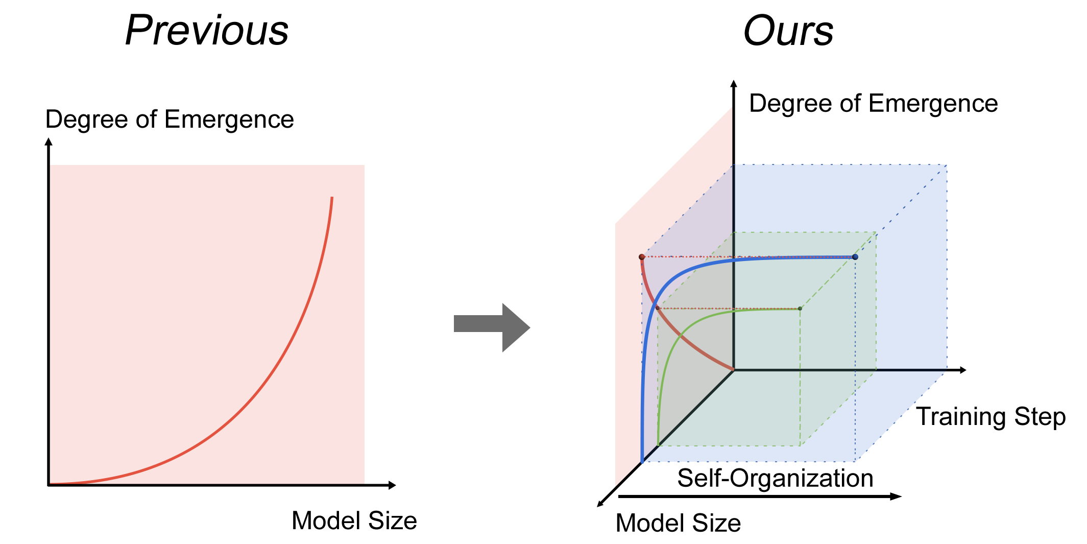
Figure 1: Difference between traditional methods and our new method. We present a different perspective of how the model gets emergence from the training steps scale.

Figure 2: Improvement of pythia responses with increasing training iterations, as indicated by the progression from incoherent to coherent answers across diverse categories (yellow for open-ended questions, blue for questions with standard answers, and red for semi-open-ended questions).

Empirical studies on analyzing the LLMs’ test performance identified power-law relationships but did not provide the intrinsic characteristics and rationale behind the emergence behavior. Previous research on the emergence in LLMs (Wei et al., 2022a; Fu et al., 2023) focused on model scale (e.g., number of parameters, model depth), but ignored the evolution of model performance during training. The iterative training process is essential for LLM development, demonstrating their evolving capabilities over time, as illustrated in Fig. 2. Large models often require more comprehensive training to achieve heightened abilities. Besides, traditional metrics (Paperno et al., 2016; Sakaguchi et al., 2021; Bisk et al., 2020) only evaluate the LLM’s output performance. Moreover, LLMs exhibit variations in their internal structures and dynamic characteristics during the training process (Ding et al., 2023). Although previous work may observe the external manifestations of emergence, they overlook the complex dynamics and internal interactions during the model training process, which are key to understanding the emergence.

Our study, therefore, extends beyond observable outcomes to explore the intricate mechanisms driving emergence in neural networks. We suggest that emergence results from the dynamic interplay and evolving complexity of neuron interactions during training, leading to sophisticated order / patterns. This mirrors the “self-organization” seen in natural systems, where simple rules at the micro-level lead to complex macro-level behaviors (see Appendix A.3). To decipher how collective neuronal interactions contribute to the self-organization and emergence phenomena during LLM’s training process, we construct a network representation of the neuronal interactions in LLMs and propose the Neuron-based Multifractal Analysis (NeuroMFA) (see Methodology 4.2) to characterize the pattern formation during these evolving interactions. NeuroMFA can learn the multiscale patterns that result from complex interactions among neurons and helps us unravel the subtle dynamics, employing a specialized weighted box covering method tailored for models’ directed weighted structure. Specifically, NeuroMFA enables precise measurement of neuron-based fractal properties and introduces the distortion factor to distinguish these structures with multiple fractal properties accounting for common and rare patterns. This multifaceted approach not only assesses the multifractal nature of neuron interactions but also deepens our understanding of the model’s training progression and the emergence of intelligence within LLMs.

In summary, the contributions of our work are three-fold: (i) We present a collective systems-inspired framework that represents LLMs as neuron interaction networks (NINs), enabling inter-neuron connectivity analysis; (ii) we introduce the neuron-based multifractal analysis (NeuroMFA) to quantify the regularity and heterogeneity of NINs, allowing us to understand neuron interactions and collective behaviors from a self-organization perspective; (iii) based on NIN and NeuroMFA, we propose a metric to measure the degree of emergence in LLMs from the perspective of neuron self-organization during the training process, opening a new direction for the study of emergence in large models.

The structure of this paper is as follows: Section 2 and 3 introduce the basic idea of emergence and self-organization, along with related work. Section 4 summarizes our NeuroMFA framework for quantifying the emergence phenomena. Section 5 presents our experiment results and analysis. Section 6 provides further discussion of our method, results and implications for future directions.

2 Emergence and Self-organization

“Emergence refers to the arising of novel and coherent structures, patterns, and proerties during the process of self-organization” (Goldstein, 1999). The emergence can be understood as the process by which new order or pattern forms - “something new appears” - in the evolution of a collective system that cannot be described by its dynamical equations, and which can be exploited by this system through various mechanisms to gain additional functionalities or capabilities (Crutchfield, 1994). In the context of LLMs, the emergence can be understood as the complex behavior by which new learning capabilities are acquired by the LLM from the collective interactions among a multitude of simple elements (i.e., the neurons which follow simple and consistent rules within the neural network). As the scale of the LLM increases, these interactions can become increasingly intricate, contributing in a synergistic way to new patterns; thus, the whole system significantly surpasses the sum of its individual parts in terms of functionality.

Self-organization is the process of pattern formation through internal interactions (Correia, 2006; Ay et al., 2007). Self-organization refers to the ability of a collective system to drive itself towards a more ordered state and maintain its functionality in the face of perturbations. Just as in natural systems where intricate patterns and behavior emerge from the interactions of individual elements following basic rules, self-organization in the context of neural networks implies the development of intricate structures and capabilities as a result of the interactions between neurons, akin to Turing Patterns where complex patterns emerge from simple rules in natural systems (see Appendix A.3.2). In contrast to prior work on observing independent LLMs at different scales, we focus on how untrained models, during training, gradually manifest increasing levels of order over multiple scales. Understanding and quantifying the degree of order-ness appearing or developing during the training of LLMs requires a strategy of estimating the rules from small data through geometric arguments (i.e., only weights of neuronal interactions are known). Towards this end, the multifractal theory (Evertsz & Mandelbrot, 1992; Salat et al., 2017; Song et al., 2005) allows us to identify rules and patterns across multiple scales.

3 Related Work

While the optimization loss decreases with increased model size, the task performance exhibits complex behavior, showing significant improvement only after a model exceeds a threshold in size, a phenomenon known as emergent abilities (EAs) (Wei et al., 2022a). Recently, the emergence has gained increasing attention in LLMs, first within the technique of ‘chain-of-thought’ on the performance of solving complex mathematical problems (Wei et al., 2022b). According to (Schaeffer et al., 2023), the scope of ‘emergence’ is defined as: 1). Large model Only: abilities that can not be found in small models; 2). Sudden change on monitored metrics: the model’s behavior has a sudden change, which means it cannot be inferred from the small model’s performance.

In emergence interpretbility area  (Fu et al., 2023),  Hu et al. introduced a quantitative evaluation strategy (i.e., PASSUNTIL), which uses massive sampling to achieve theoretically infinite resolution. Derived from the quantization hypothesis,  Michaud et al. presented the quantization model for neural scaling laws, which aims to explain the observed power-law decrease in loss concerning model and data size, as well as the phenomenon of EAs with scale.  Gurnee et al. investigated the concept of universal neurons in GPT-2 language models, finding that a small percentage of neurons are universal, exhibiting consistent behavior across models trained with different random seeds. In contrast,  Schaeffer et al. challenged the notion of EAs in LLMs and proposed that the appearance of emergent abilities is influenced by the choice of evaluation metrics rather than actual changes in model behavior.

Furthermore, LLMs (e.g., ChatGPT, LLaMA) encounter limitations in domain-specific tasks. They often lack depth and accuracy in specialized areas, and exhibit a decrease in general capabilities when fine-tuned, particularly analysis ability in small sized models (Gaur & Saunshi, 2023; Zheng et al., 2024; Chan et al., 2023). According to Wei et al. (2023), smaller LLM relies primarily on semantic priors from pretraining when presented with flipped in-context labels, whereas larger models can override priors, demonstrating reduced reliance on semantic priors even with potentially stronger priors due to larger scale. Jaiswal et al. proposed the existence of essential sparsity when directly removing weights with the smallest magnitudes in one-shot without re-training. While prior work observed emergent outcomes, the complex internal dynamics and evolving interactions during training remain overlooked. In this work, we argue that understanding emergence requires investigating the neuronal-level processes whereby self-organization arises from initially random interactions as training progresses.

4 Methodology

4.1 LLMs’ Neurons as Interacting Agents in a Network

To illustrate our method, let us define the components of a neural network (NN). Let $N$ denote a neural network. $N$ is composed of several blocks $B_{1},B_{2},\cdots,B_{k}$. Each block $B_{i}$ contains multiple layers $L_{1}^{i},L_{2}^{i},\cdots,L_{m_{i}}^{i}$. Each layer $L_{j}^{i}$ comprises multiple neurons $n_{1}^{ij},n_{2}^{ij},\cdots,n_{p_{ij}}^{ij}$. Neurons between layers are interconnected by weights $w_{ab}\in W$, where $a$ and $b$ denote the indices of the neurons. There are no connections between neurons within the same layer.

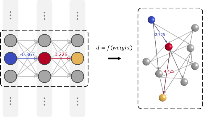
Figure 3: The transformation from a neural network to a neural interaction network.

Figure 4: (a) shows examples of our weighted box covering method, illustrating two neurons randomly selected from the NIN of pythia 1B model at the $143,000^{th}$ epoch. The radius of each box, $r$, is determined by the distance to its neighboring neurons, with $N$ representing the number of neurons contained within a box. (b) demonstrates the power-law relationship between $N$ and $r$.

The structure of a NN provides information about its architecture and connections. Consequently, our proposed multifractal analysis investigates the interactions among neurons, with a specific emphasis on identifying the shortest paths or distances. In NNs, larger weights typically indicate stronger interactions, suggesting shorter distance between two neurons in our network analysis. This motivates us to transform the NN into a so called “Neuron Interaction Network”, defined as follows.

Definition 4.1 (Neuron Interaction Network (NIN)).

NIN is a directed weighted graph $G=(V,E)$ with a weight transfer function $f$, where:

[1]. $v\in V$ denotes the set of neurons in the NN; since nodes in the NIN are the same as those in the NN, we do not differentiate between them in this article;

[2]. $e_{a,b}\in E,(a,b\in V)$ represents a link between original neurons, with a new weight $d_{ab}$ determined by $f$;

[3]. $f:\mathcal{R}\rightarrow\mathcal{R}$ decides the edge distance in the NIN, being calculated based on original weights among neurons;

[4]. Blocks $B$ and layers $L$ are preserved by the NIN structure.

We assume that the function $f$ has the property of Absolute Value and Decreasing, where the absolute value escapes the influence of the negative output on weight calculation, and decreasing indicates we only target the shortest path for analysis. Thus, we formulate $f$ as follows:

$$f(w_{ij})=\begin{cases}\frac{1}{|w_{ij}|},&\text{if }w_{ij}>\epsilon\\ 0,&\text{otherwise}\end{cases},\forall i,j\in V$$ (1)

where $\epsilon$ is the threshold of weights, $w_{ij}$, for this quantifiable network model to guarantee the sparsity. We also explore different functions $f$ and provide the ablation studies in section Section 5.4.

Since LLMs contain a huge number of neurons, it is inefficient to do the analysis on the whole NIN. To this end, we define a Sampled Neural Interaction Network to improve the analysis efficiency.

Definition 4.2 (Sampled Neural Interaction Network (SNIN)).

A SNIN represents a sampled subgraph $G^{\prime}=(V^{\prime},E^{\prime})$ of the original NIN. In each layer $L_{i}$, we sample a subset of nodes $V_{i}^{\prime}\in L_{i}$, and add them to SNIN and having weights $E^{\prime}=\{e_{ab}|e\in E,a,b\in V^{\prime}\}$.

To enhance the precision and efficiency on NIN analysis, we adopt a strategy where we average the outcomes from analyses of 10 randomly selected SNIN sets in NIN. As substantiated in Section A.1.2, this sampling methodology does not alter the estimation of the fractal dimensions. For clarity and simplicity, we consistently use the notation $G=(V,E)$ and refer to the NIN instead of SNIN in subsequent sections.

4.2 Neuron-based Multifractal Analysis (NeuroMFA)

To perform multifractal analysis of LLMs, we extend the box-covering and box-growing methods (Song et al., 2005; Xiao et al., 2021) to capture the local (based on each neuron) fractal properties of NINs. Specifically, let us consider neuron $v_{i}$ as a box with an initial radius of zero at layer $l$ and indexed by $i$. We then increase the radius of the box and record the mass distribution (i.e., the number of nodes covered by the box). First, we define $N_{l,i}(r)$ as the number of neurons connected to neuron $v_{l,i}$ within a radius $r$. For a specific neuron $v_{i}$ at layer $l$ and radius $r$, $N_{l,i}(r)$ is calculated as follows:

$$N_{l,i}(r)=\sum_{v_{j}\in L_{l+1}}\mathbf{1}_{\{d_{ij}\leq r\}},$$ (2)

where, $\mathbf{1}_{\{d_{ij}\leq r\}}$ is an indicator function that takes the value 1 when the distance between neuron $v_{i}$ and $v_{j}$, $d_{ij}$, is less than or equal to $r$, and 0 otherwise. Thus, $N_{l,i}(r)$ computes the number of neurons in the next layer(s) connected to neuron $v_{i}$ within the radius $r$.

The process continues with increasing the box radius until all the neighbors of the neuron are covered. The method captures the log-log relationship between the box radius $r$ and the mass distribution $N_{l,i}(r)$ in the box, and indicates the fractal properties of the neuron interactions (see Figure 4 and Table 2, Section C.1.4).

Observation 4.1.

In a NIN, the relation between the mass distribution $N(r)$ and box radius $r$ can be expressed as:

$${N(r)}\sim r^{D},$$ (3)

where $D$ denotes the fractal dimension characterizing the fractal properties of the interactions among a neuron and its neighbors.

To capture the multifractality of the neuron interactions, we develop the NeuroMFA framework. This method integrates the fractal features of different neurons in the NIN. The distortion factor $q$ is introduced to differentiate the nuances of fractal structural features. For a given neuron $v_{i}$ at layer $l$ in the neural network $G=(V,E)$, the mass probability measure $p_{l,i}(r)$ at a radius $r$ is defined as:

$$p_{l,i}(r)=\frac{N_{l,i}(r)}{T_{l,i}}$$ (4)

where $N_{l,i}(r)$ is the number of neurons within the radius $r$ from neuron $v_{i}$, and $T_{l,i}$ is the total number of neurons in layer $l+1$ that are connected to neuron $v_{i}$.

Definition 4.3 (Partition Function).

The partition function $Z_{q}(r)$ for the neuron-based multifractal analysis is defined as the sum of the $q$-th power of the probability measures across all neurons in the network, given by:

$$Z_{q}(r)=\sum_{l=1}^{L}\sum_{v_{i}\in L_{l}}p_{l,i}(r)^{q}$$ (5)

We provide the algorithm to obtain the partition function in Appendix Algorithm 5.

Observation 4.2.

A log-log relationship exists between $Z_{q}(r)$ and the observational scale $r/d$, validated in Table 2, Section C.1.4:

$$Z_{q}(r)\sim\left(\frac{r}{d}\right)^{\tau(q)},$$ (6)

where $d$ is the maximum box radius and $\tau(q)$ is the mass exponent.

Lemma 4.1 (Multifractal Scale Invariance).

Let $\mu$ be a mass probability measure defined on the network. For any positive number $q$ and scale $\epsilon$, if there exists a constant $C(q)$ such that

$$\sum_{i}[\mu(B_{i}(\epsilon))]^{q}\approx C(q)\epsilon^{\tau(q)},$$ (7)

then the network is said to possess multifractal scale invariance. Here, $B_{i}(\epsilon)$ represents the box of scale $\epsilon$, and $\tau(q)$ is the mass exponent.

Algorithm 1 Calculation of the Mass Exponent $\tau(q)$ in Eqn. 6

0:  $r_{\text{sorted}}$ (a list of sorted box radius, output from Algorithm 5), $Zq_{\text{list}}$ (a list of Partition functions, output from Algorithm 5), $d$ (maximum of box radius)

1:  for all $Zq$ in $Zq_{\text{list}}$ do

2:      Calculate the slope of the linear regression of $\log(Zq)$ on $\log\left(\frac{r_{\text{sorted}}}{d}\right)$

3:     Save the slopes to an empty list: $\tau_{\text{list}}$

4:  end for

5:  return $\tau_{\text{list}}$

Definition 4.4 (Multifractal Spectrum).

The Legendre transform enables the computation of the the Lipschitz-Hölder exponent $\alpha(q)$ and multifractal spectrum $f(\alpha)$ characterizing the multifractal structural features of the network:

$$\alpha(q)=\frac{d\tau(q)}{dq},$$ (8)

$$f(\alpha)=q\alpha(q)-\tau(q),$$ (9)

We provide the algorithm to obtain the partition function in Algorithm 2.

Algorithm 2 Calculation of the Multifractal Spectrum $f(\alpha)$ in Eqn. 9

0:  $\tau_{\text{list}}$ (a list of mass exponents, output from Algorithm 1), $q_{\text{list}}$ (a list of distortion factors)

1:   Calculate the $\alpha_{\text{list}}$ using Eqn.8 $\alpha_{\text{list}}\leftarrow\frac{d\tau_{\text{list}}}{dq_{\text{list}}}$

2:   Calculate the $f(\alpha)_{\text{list}}$ using Eqn.9 $f(\alpha)_{\text{list}}\leftarrow q_{\text{list}}\cdot\alpha_{\text{list}}-\tau_{\text{list}}$

3:  $\alpha_{0}\leftarrow$ $\alpha_{\text{list}}$ [index of maximum value in $f(\alpha)_{\text{list}}$]

4:  $\text{width}\leftarrow\max(\alpha_{\text{list}})-\min(\alpha_{\text{list}})$

5:  return $(\alpha_{0},\text{width},\alpha_{\text{list}},f(\alpha)_{\text{list}})$

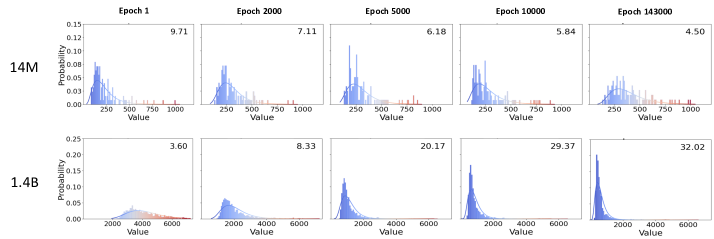
Figure 5: The distributions of average weighted degree for two models of different sizes during the training process. The number in the figure represents Kurtosis, indicating the distribution’s tail weight and peak sharpness. High kurtosis implies heavier tails and a sharper peak, whereas low kurtosis suggests lighter tails and a flatter peak.

4.3 Degree of Emergence

While the Lipschitz–Hölder exponent $\alpha$ provides information about the nature of regularity / order and singularity, the multifractal spectrum $f(\alpha)$ offers insight into the frequency (commonly or rarely occurring pattern) and thus can help us quantify the complex and heterogeneous nature of a weighted network topology. Here we extract measures from the multifractal spectrum to quantify the regularity and heterogeneity of network structures, and use these to construct our measure for the degree of emergence.

Definition 4.5 (Regularity Metric $\alpha_{0}$).

The exponent $\alpha_{0}$ is defined as the Lipschitz–Hölder exponent value $\alpha$ at which the multifractal spectrum $f(\alpha)$ attains its maximum, i.e.,

$$\alpha_{0}=\arg\max_{\alpha}f(\alpha).$$ (10)

The exponent $\alpha_{0}$ represents the most prevalent degree of singularity within the network, and a higher value of $\alpha_{0}$ indicates a greater level of irregularity and complexity in the network’s structure. Therefore, we employ $\alpha_{0}$ as a metric for assessing the NIN’s regularity. A more detailed explanation is provided in Section A.2.1.

Definition 4.6 (Heterogeneity Metric $w$).

The width $w$ of the multifractal spectrum is defined as the difference between the maximum and minimum values of the Lipschitz–Hölder exponent $\alpha$, represented by

$$w=\alpha_{\text{max}}-\alpha_{\text{min}}.$$ (11)

This width $w$ measures the heterogeneity of the network, with a larger value indicating a broader range of fractal structures within the network. Further details are provided in Section A.2.2.

To quantify the emergence, which are critical for understanding the learning process in LLMs, we estimate the order / regularity $\alpha_{0}(t)$ and heterogeneity $w(t)$ at epoch $t$ from their corresponding network representation.

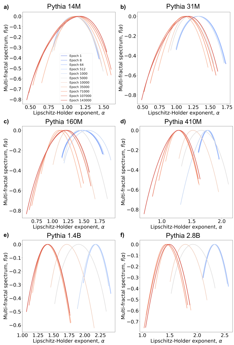
Figure 6: Multifractal spectra of Neuronal Interaction Networks (NINs) for models of varying sizes throughout the training process.

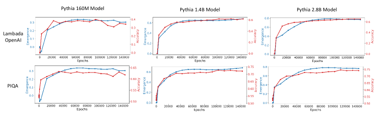
Figure 7: The comparison between our proposed metric with two metrics.

Definition 4.7 (Degree of Emergence).

The degree of emergence can be calculated through the following formula:

$$E=\frac{w(t)}{w(0)}\log\left(\frac{\alpha_{0}(0)}{\alpha_{0}(t)}\right)$$ (12)

This formula integrates the changes in heterogeneity and regularity over time, where $\frac{w(t)}{w(0)}$ signifies the relative change in heterogeneity, i.e., diversity in network structures, and $\log\left(\frac{\alpha_{0}(0)}{\alpha_{0}(t)}\right)$ represents the change in regularity, providing a normalized view of structural shifts. The product of these terms yields a comprehensive measure of network’s evolving complexity and organization, offering insights into the nature and degree of emergence within the system. See Section A.2.3 for a more complete explanation.

5 Experiment

In this section, we describe the experiments conducted for analyzing the NINs to observe the self-organization process during training and evaluating our new metrics. Our experiments are conducted on Pythia (Biderman et al., 2023) models (except for specific requirements like different architectures). Pythia models provide checkpoints during training phases and different model scales, which is helpful for us to reveal the rules behind these scales of training step and model size.

5.1 Average weighted degree distribution

Previous work has reported the existence of heavy-tail degree distributions in the node connectivity of neural networks, which suggests the presence of hubs, playing an important role in the network (Barabási & Bonabeau, 2003; Broido & Clauset, 2019). These phenomena are commonly considered as outcomes of self-organization (Park et al., 2005; Evans & Saramäki, 2005).

In our work, we first construct NINs for two versions of the pythia model: a small-scale 14M parameter model (pythia 14M) and a larger 1.4B parameter model (pythia 1.4B). Dealing with NINs, we compute the weighted degree of each node, defined as the average value of distances from connections. This allows us to analyze the average weighted degree distributions that emerge during training.

Figure 5 shows a clear distinction between the two models. During the training process, the average degree distribution for pythia 14M exhibits a dispersed trend, with lower kurtosis values (where kurtosis is commonly used to measure distribution characteristics, with higher kurtosis indicating a heavier-tailed distribution, see Section A.4), the distribution for pythia 1.4B with left shifting indicates the trend of appearing a heavy-tail distribution over multiple epochs of pertaining, which is also indicated by the increasing Kurtosis value. Please refer to Section C.4 for more information and results of Kurtosis value on pythis 14M, 160M, and 1.4B. This indicates that as the scale of the model increases, the average distance from most neurons to the neighbors in the next layer decreases, signifying the establishment of stronger interactions. It might imply that an organizational structure with a heavy-tailed connectivity pattern systematically self-organizes. Therefore, further in-depth research into the network’s connectivity structure is required to observe the self-organization process, leading us to the multifractal analysis of the network.

5.2 The Self-organization Process of the LLM Networks

We analyze the dynamic LLM networks during their training process. The self-organization process, characterized by the emergence of new patterns and increasingly organized structures, can be quantitatively assessed using the $w$ and $\alpha_{0}$ metrics from Section 4.3. For each model with different sizes, NeuroMFA is applied to networks at various epochs. The curves showing the changes in the values of $\alpha_{0}$ and $w$ with epochs are provided in Fig. 14. The spectra, which vary with the epochs, exhibit distinct behaviors that reveal certain trends, as discussed below.

Increasing Heterogeneity. The spectrum width $w$ measures the degree of heterogeneity of the network. Figure 6 shows that $w$ tends to broaden with more training epochs. This widening, evident from the initial spectrum to later stages, signals an increasing heterogeneity in the network’s structure. This phenomenon is largely due to the emergence of varied fractal patterns, which are intricate structures formed through neuronal interactions during training. These patterns contribute to the spectrum width’s expansion.

The analysis of relatively smaller networks, ranging in size from 14M to 410M parameters, reveals a consistent trend: the spectrum width $w$ increases steadily. However, an interesting deviation occurs in larger models exceeding 1 billion parameters. After approximately 35,000 training epochs, the spectrum width stabilizes, suggesting that the network’s fractal diversity reaches a sort of equilibrium at this stage.

In addition, as shown in Fig. 6, the spectra become wider with increasing epochs, suggesting an increase in the heterogeneity of the network structure. This widening is attributed to the formation of more interactions exhibiting different fractal patterns during the training process, thus broadening the spectrum.

Decreasing Regularity. In network analysis, a leftward shift of the multifractal spectrum indicates self-organization. This shift suggests an increase in the network’s regularity, as marked by a decrease in the $\alpha$ parameter. However, Fig. 6 (a) shows for smaller model (e.g., 14M) an increasing trend of $\alpha_{0}$. As training progresses through epochs, the spectrum tends to shift rightward slightly instead of leftward. This indicates that, in the 14M model, the network’s regularity does not decrease. Similarly, the 31M model displays a subtle leftward shift at the 5,000th epoch, but this trend does not continue significantly thereafter.

In contrast, for larger models (exceeding 100M parameters), a consistent leftward shift of the network spectra is observed from the 0th to the 35,000th epoch. This shift suggests an increase in regularity and a corresponding enhancement in self-organization as training progresses. After reaching the 3,5000th epoch, this leftward shift in the spectrum stabilizes across these larger models. This stabilization implies that further increases in training epochs do not significantly affect the network’s degree of regularity. This could indicate that the model training has reached a certain threshold, beyond which no additional self-organization is observed.

5.3 Quantitative Analysis of Emergence

In this section, we assess the degree of emergence $E$ for LLMs during the training process. Figure 7 shows the emergence analysis across models of varying scales (160M, 1.4B, 2.8B) and their performance for different benchmarks. We observe a positive correlation, i.e., higher levels of emergence are associated with enhanced expected model performance, as evidenced by increases in testing accuracy; of note, we acknowledge that this is restricted to these datasets and a more comprehensive evaluation should be done across more datasets (see more results across different metrics in Section C.3).

Data from Lambada and PIQA tests reveal a significant increase in model accuracy during the initial training phase, up to approximately the 15,000th epoch. This trend was paralleled by a swift increase in $E$. From around the 15,000th to the 40,000th epochs, we noted a gradual enhancement in model performance, aligning with the trajectory of the degree of emergence $E$. Post this phase, models tend to stabilize, exhibiting fluctuating accuracies. These fluctuations mirrored the emergence levels, further validating our metric.

Moreover, we observe significant performance oscillations in two other datasets (WSC and LogiQA, see Section C.3), suggesting their limited utility in assessing model capabilities. This underscores the limitations of relying solely on performance metrics for evaluating model’s emergence. Therefore, our approach to studying emergence focuses on analyzing the model itself, rather than merely its output or performance. This methodology provides a more comprehensive view of the emergence phenomenon in LLMs, encapsulating both the intricacies of the training process and the nuanced evolution of the model. Information about the benchmarks can be found in Appendix  B.3.

5.4 Impact Evaluations

Next, we will introduce ablation experiments to investigate the effect of various designs on the emergence metric.

Varing weight transfer functions. In Section 4.1, we choose a specific weight transfer function $f$ which satisfies the property requirements. Here, we discuss if different choices of $f$ influence the analysis results. As observed, we found $\forall w\in W,0<w\leq 1$. Based on this, we choose the following alternative functions: 1).$f(w)=\coth(|w|)$ 2). $f(w)=|\log(|w|)|$ (the $\epsilon$ part remains the same).

Full analysis results can be found in Appendix C.1.1. From these results, we can see that if $f$ satisfies the property requirement we mentioned in Section 4.1, it will not influence the analysis conclusions.

Varying tasks. Although in the area of computer vision (CV) several generative models (Rombach et al., 2022) providing personalized image generation exhibit a potential degree of intelligence, no analysis of their degree of emergence exists. Thus, we conduct an emergence analysis on these models. The experimental results can be found in Appendix C.1.2. The degree of emergence for CV tasks is lower than the NLP tasks at the same parameter size, which indicates a lower level of intelligence. This may explain why CV models have not found emergence yet.

Varying layer interactions. Our neural-based MFA approach differs significantly from traditional network analysis methods in that it accounts for the directed hierarchical structure of NIN. We initially assess the local fractal properties revealed by neurons’ neighboring mass distribution.We also explored connections across multiple layers (2 and 3 layers), but the computational load was substantial, the calculation and estimation algorithms can be found at Appendix B.1. The corresponding results are presented in Appendix C.1.3. Fractal analysis at a single layer shows more pronounced changes across different epochs, demonstrating heightened sensitivity to fractal characteristic variations. Including two or three layers complicates the analysis by introducing more nodes, which might disturb the neighboring fractal rules and obscure structural changes. This complexity underscores the advantage of our method, emphasizing its ability to discern subtle shifts in structure that multi-layer analyses may miss, thereby confirming our approach’s effectiveness in capturing fractal dynamics.

6 Discussion and Conclusion

Our novel emergence framework effectively elucidates the interplay between model scale, training steps, and performance, offering a cohesive explanation for the learning evolution in LLMs. Looking ahead, this methodology holds potential not only for enhancing interpretability and assessment, but also for forecasting LLM’s behavior and their subsequent developments. Recent findings by (Bubeck et al., 2023) suggest that current LLMs represent an initial step towards Artificial General Intelligence (AGI). Leveraging our approaches, we might be able to anticipate the conditions necessary for the next leap in model intelligence by our new measurement, potentially marking the threshold for AGI.

.tocmtappendix mtchapternone mtappendixsubsection

Appendix A Theories and Methodology Details

A.1 Multifractal Analysis

A.1.1 Hausdorff Measure

The Hausdorff measure is a key concept in fractal geometry and measure theory, extending the notion of Lebesgue measure to irregular sets, particularly useful for characterizing the size of fractals. It’s named after Felix Hausdorff, a pioneer in set theory and topology.

Formally, consider a set $A\text{ within }\mathbb{R}^{n}$. For a metric space $\displaystyle(X,\rho)$, the diameter of $U$ is defined as:

$$\text{diam}U:=\sup\{\rho(x,y):x,y\in U\},\text{diam}\varnothing:=0,$$ (13)

where $U$ is any subset $U\subset X$.For $\delta>0$, define the $\delta$-approximate $d$-dimensional Hausdorff measure as:

$$\mathcal{H}^{d}_{\delta}(A)=\inf\left\{\sum_{i=1}^{\infty}(\text{diam}(U_{i}))^{d}:\bigcup_{i=1}^{\infty}U_{i}\supseteq A,\text{diam}(U_{i}))^{d}<\delta\text{ (}\{U_{i}\}\text{ is a }\delta\text{-cover of }A\text{)}\right\}$$ (14)

where $\text{diam}(U_{i})$ is the diameter of the set $U_{i}$, and a $\delta$-cover is a countable collection of sets $\{U_{i}\}$ covering $A$ with $\text{diam}(U_{i})<\delta$ for all $i$. The $d$-dimensional Hausdorff measure of $A$ is then defined as the limit of $\mathcal{H}^{d}_{\delta}(A)$ as $\delta$ approaches zero:

$$\mathcal{H}^{d}(A):=\sup_{\delta>0}\mathcal{H}^{d}_{\delta}(A)=\lim_{\delta\to 0}\mathcal{H}^{d}_{\delta}(A)$$ (15)

The Hausdorff dimension $\dim_{H}(A)$ of a set $A$ is defined as the infimum over all $d$ such that the $d$-dimensional Hausdorff measure of $A$ is zero:

$$\dim_{H}(A)=\inf\{d\geq 0:\mathcal{H}^{d}(A)=0\}.$$ (16)

Equivalently, it can be described as the supremum over all $d$ such that the $d$-dimensional Hausdorff measure of $A$ is infinite:

$$\dim_{H}(A)=\sup\{d\geq 0:\mathcal{H}^{d}(A)=\infty\}.$$ (17)

This dimension is a critical value that separates the scales at which the set $A$ appears “large” from those at which it appears “small” in terms of its $d$-dimensional Hausdorff measure. It provides a precise mathematical way to quantify the notion of dimension for irregular sets, like multifractals, which do not fit neatly into the traditional framework of integer dimensions.

A.1.2 Multifractal Analysis by Box-counting Method

In the domain of network analysis, multifractal analysis (Song et al., 2005, 2007; Furuya & Yakubo, 2011) employs the box-counting method to elucidate the intricate, multifractal structures inherent in complex networks. This analytical approach aligns with the renormalization procedure, essential for understanding multifractality within these systems. The process commences with covering the network using a series of boxes of variable sizes, denoted as $\epsilon$. The count of boxes, $N(\epsilon)$, required to encompass the network at each scale is meticulously recorded. This methodology resonates with the principles of renormalization, highlighting the dynamic interplay between different scales within the network. This approach is akin to assessing the Hausdorff measure A.1.1, a foundational concept in fractal geometry that quantifies the size of a fractal object. Here we provide the process of the calculation of the gerneralized fractal dimension and the multifractal spectrum.

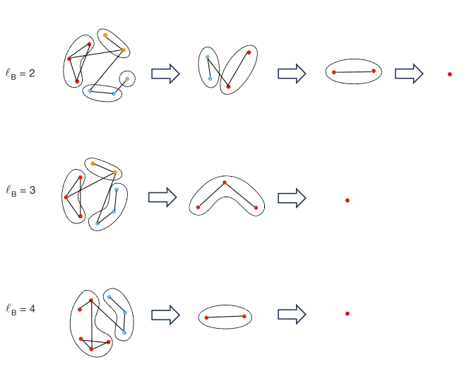
Figure 8: This figure illustrates the renormalization procedure in network theory. It demonstrates the systematic reduction of a network’s scale by grouping nodes within a specified linkage distance, $l_{B}$ into single representative nodes, or ‘boxes’. Each color represents a different box. When two nodes from different original boxes are connected by an edge, the corresponding renormalized nodes are connected as well. This process is iteratively applied, progressively coarsening the network, until it is reduced to a single node. This figure is similar with Figure 1 (a) in (Song et al., 2005).

The fractal structure is divided into boxes (or elements) of size $\epsilon$. Each box covers a part of the fractal, with a total of $N(\epsilon)$ boxes. The renormalization process is illustrated in Fig. 8. For each box, we calculate the proportion of the mass probability measure within that box, denoted as $p_{i}$, where $i$ represents the $i$-th box. By applying a $q$-th power weighting to the probability $p_{i}$ in each box, we obtain the partition function $\sum_{i=1}^{N(\epsilon)}p_{i}^{q}$. The distortion factor $q$ can adjust the relative importance of different box probabilities. Considering the scale factor as $\epsilon$ approaches 0 to capture the fractal, the generalized fractal dimension is calculated as:

$$D_{q}=\frac{1}{q-1}\lim_{\epsilon\to 0}\frac{\log\sum_{i=1}^{N(\epsilon)}p_{i}^{q}}{\log\epsilon}$$ (18)

Subsequently, through Legendre transform, the Lipschitz-Hölder exponent $\alpha(q)$ is determined through the differential equation:

$$\alpha(q)=\frac{d}{dq}((q-1)D_{q})$$ (19)

This exponent $\alpha(q)$ provides insights into the local regularity of the network structure at various scales. Advancing this analytical framework, the multifractal spectrum $f(\alpha)$ is derived from the relationship:

$$f(\alpha)=q\alpha-((q-1)D_{q})$$ (20)

The multifractal spectrum $f(\alpha)$, in conjunction with $\alpha(q)$, offers a comprehensive understanding of the network’s scaling behaviors, revealing the multifractal and heterogeneous nature of its structure. This spectrum delineates the distribution of singularities across the network, thus encapsulating the essence of multifractality. The utilization of these calculations in network analysis is not merely computational; they provide profound insights into the network’s heterogeneity, unraveling the multifractal core of its structure and the dynamics that shape its evolution.

A.1.3 Power Law in fractal dimension

The definition of fractal dimension is based on unconventional views of scaling and dimension. In conventional geometry, dimension can be defined by intuitive space scaling law. For example, a line with finite length can contain 3 lines with 1/3 its size. But for a square, with a box of side length 1/3 the size of a square, one will find 9 times as many squares as with the original. In general, mathematical definition of such scaling law can be given by

$$N=\varepsilon^{-D},$$ (21)

where $N$ stands for the number of measurement units, $\varepsilon$ is the scaling factor. Thus this gives the definition of dimension D:

$$D=-\log_{\varepsilon}N=-\frac{\ln N}{\ln\varepsilon}.$$ (22)

For lines we can see $N=3$ when $\varepsilon=\frac{1}{3}$. Then we get $D=1$. In the case of a square $D=2$ because $N=9$ when $\varepsilon=\frac{1}{3}$.

Then the definition can be generalized into fractal geometry. For example, the Koch snowflake shown in fig.9, $N=4$ when $\varepsilon=\frac{1}{3}$. Thus the fractal dimension $D=\log_{3}4\approx 1.2618595$, which is not a integer. Even though it is not intuitive any more, the scaling law $N=\varepsilon^{-D}$ still exists. Then for fractal objects embedded in the Euclidean space we can use box-covering method to define fractal dimensions, which is useful for fractal networks:

$$N_{B}(r_{B})\sim r_{B}^{-D},$$ (23)

where $N_{B}(r_{B})$ is the minimum number of boxes needed to tile a given fractal network with the box radius $r_{B}$. Then we can define the fractal dimension in another way. The mass distribution is defined by the average number of vertices $\langle N(r_{C})\rangle$ within a box with radius $r_{C}$. The mass-radius relation can be given when the relation $M\sim N_{B}(r_{B})\langle N(r_{C})\rangle$ holds for $r_{B}=r_{C}=r$. Then we can characterize the power law between the mass distribution $N(r)$ and the box radius $r$ as

$$N(r)\sim r^{D},$$ (24)

where $D$ is the fractal dimension.

Lemma A.1 (Scale Invariance).

Let $\mu$ be a mass measure defined on the network. For any radius $\epsilon$ around a specific node, if there exists a constant $C$ and a real number $D$ such that the following relationship holds:

$$\mu(B(\epsilon))\approx C\epsilon^{D},$$ (25)

where $B(\epsilon)$ is the set of nodes within radius $\epsilon$ of the specified node, then the network exhibits scale invariance at the local scale around the node. $D$ represents the local fractal dimension.

Definition A.1 (Neuron-based Fractal Dimension).

Consider a neuron $v_{i}$ in the layer $l$ of the NIN. The neuron-based fractal dimension $D_{l,i}$ is defined to capture the fractal characteristic based on each neuron. Given the set of distances $\{r_{1},r_{2},...,r_{m}\}$ from $n_{l,i}$ to its neighbors in the next layer $l+1$, the fractal dimension $D_{l,i}$ is calculated as follows:

$$D_{l,i}=\frac{\sum\limits_{k=1}^{m}(\log(r_{k})-\bar{\log(r)})(\log(N_{l,i}(r_{k}))-\bar{\log(N_{l,i}(r))})}{\sum\limits_{k=1}^{m}(\log(r_{k})-\bar{\log(r)})^{2}}$$ (26)

where $r_{k}$ represents each distances in the set, $N_{l,i}(r_{k})$ is the number of neurons within the distance $r_{k}$, and $\bar{\log(r)}$, $\bar{\log(N_{l,i}(r))}$ are the mean values of $\log(r_{k})$ and $\log(N_{l,i}(r_{k}))$, respectively.

In practice, to calculate the fractal dimension of a large network we do not need to count all nodes. A practical method is to randomly sample the nodes in the box. Note that when we plot a $\ln{r}-\ln{N}$ graph, the slope is the fractal dimension $D$:

$$\ln N=D\ln r.$$ (27)

When we randomly sample the nodes with a constant ratio $k$, it only generates a constant intercept compared to the original:

$$\ln N^{\prime}=\ln kN=\ln N+\ln k=D\ln r+\ln k,$$ (28)

where $\ln{k}$ is a constant. Then we can still calculate the fractal dimension from its slope.

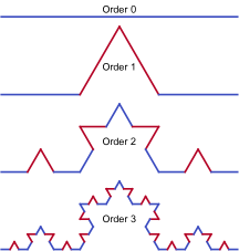
Figure 9: Fractal pattern.

A.2 Elaboration for NeuroMFA

A.2.1 Lipschitz-Hölder Exponent

In the context of multifractal analysis, the Lipschitz-Hölder exponent, denoted as $\alpha$, is crucial for characterizing the local scaling properties of a dataset. Mathematically, $\alpha$ is defined as the derivative of the mass exponent $\tau(q)$ with respect to $q$, expressed as $\alpha(q)=\frac{d\tau(q)}{dq}$. Here, $\tau(q)$ represents the mass exponent that characterizes the scaling behavior of the data at different moments ($q$).

The value of $\alpha$ provides insights into the degree of irregularity at various scales within the dataset. Lower values of $\alpha$ suggest a higher level of regularity, where the data exhibits smoother transitions and less variability in its local structure. In contrast, higher values of $\alpha$ are representative of regions with more irregular and disordered scaling behavior. This distinction is fundamental to multifractal analysis, offering a detailed perspective on the heterogeneous nature of the data and its scaling properties across various scales.

Therefore, the distribution and range of $\alpha$ values within the multifractal spectrum offer valuable insights into the underlying scaling dynamics of the dataset, revealing the intricate interplay between uniformity and complexity that defines its multifractal nature.

A.2.2 Spectrum Width

The spectrum width, denoted as $w$, in multifractal analysis plays a pivotal role in quantifying the heterogeneity of a network’s structure. It is defined as the difference between the maximum and minimum values of the Lipschitz-Hölder exponent $\alpha$, mathematically expressed as $w=\alpha_{\text{max}}-\alpha_{\text{min}}$.

This width $w$ captures the range of scaling behaviors exhibited by the network across different regions. A larger $w$ indicates a broader spectrum of $\alpha$ values, signifying a network with a wide variety of scaling behaviors. Such diversity in scaling properties points to a network with a rich mixture of regular and irregular structures, highlighting the complexity and variability in its composition.

In essence, the spectrum width $w$ serves as a crucial metric for assessing the structural heterogeneity of a network. It reflects the degree to which the network deviates from uniform scaling behavior, offering insights into the multifaceted and complex nature of the network’s fractal characteristics. The broader the spectrum, the more pronounced the heterogeneity, revealing a network structure that is rich in its diversity.

A.2.3 Degree of Emergence

In the study of self-organizing networks, the phenomenon of emergence is a key concept, representing the evolution from simpler initial states to more complex and ordered structural patterns. The measure of emergence, denoted as $E$, aims to quantify this transition from disorder to order, capturing the key characteristics of the network’s self-organization process.

The measure of emergence $E$ considers two principal aspects: the increase in network regularity and the growth in heterogeneity. Regularity, indicated by the parameter $\alpha_{0}$, reflects the uniformity and predictability of the network’s structure. As the process of self-organization progresses, changes in $\alpha_{0}$ suggest a transition of the network structure towards greater regularity and consistency. This transition is typically marked by an increase in uniform patterns, indicating a move from a more irregular to a more regular state.

Heterogeneity, represented by the parameter $w$, illustrates the diversity of the network’s fractal structure. A larger $w$ value points to a network exhibiting a variety of structural characteristics across different regions. The emergence of new patterns and structures during self-organization leads to an increase in $w$, reflecting a rise in the diversity and heterogeneity of the network’s structure.

Thus, the emergence measure $E$ is defined as:

$$E=\frac{w(t)}{w(0)}\log\left(\frac{\alpha_{0}(0)}{\alpha_{0}(t)}\right)$$ (29)

This metric accounts for the relative changes in regularity and heterogeneity over time, offering a comprehensive perspective to quantify the phenomenon of emergence in the network’s self-organization. In this formula, $\frac{w(t)}{w(0)}$ represents the relative change in heterogeneity, while $\log\left(\frac{\alpha_{0}(0)}{\alpha_{0}(t)}\right)$ captures the relative change in regularity. The utilization of the logarithm function is crucial, as it allows the emergence measure to have positive or negative values, reflecting whether the multifractal spectrum shifts left or right, a critical indicator of emergence in the model. By integrating these dimensions, $E$ effectively describes the network’s evolution from its initial state to a more advanced level of organization, revealing the complex dynamics and characteristics of emergence in the self-organizing process.

A.3 More Discussion on ‘Self-organization’

A.3.1 Emergence and Self-organization

Emergence and self-organization are fundamental concepts that span across multiple disciplines, including physics, biology, computer science, and sociology, among others. They describe the way complex systems and patterns arise out of a multiplicity of relatively simple interactions.

Emergence. Emergence refers to the phenomenon where larger entities, patterns, or regularities arise through interactions among smaller or simpler entities that themselves do not exhibit such properties. The essential point about emergent properties is that they are not properties of any component of the system but of the system as a whole.

Self-organization. Self-organization is closely related to emergence and is often seen as a process leading to emergent properties. It is the process by which a system, without external guidance, spontaneously forms a coherent and ordered structure.

Emergence and self-organization underpin complex systems across physics, biology, computer science, and sociology. Emergence captures how complex systems and patterns spring from simple interactions. Self-organization, integral to emergence, describes systems spontaneously forming ordered structures without external direction. In Physics, emergence is seen in phenomena like thermodynamics, where macroscopic properties such as temperature and pressure emerge from the collective behavior of particles(Epstein et al., 2006). Self-organization is observed in non-equilibrium processes such as the formation of crystal structures or the spontaneous formation of cyclones in the atmosphere. In Biology, emergence explains how complex biological phenomena, such as life, arise from the interactions of non-living molecules in the right conditions(Kauffman, 1993). The behavior of ant colonies, where complex organization and problem-solving abilities emerge from simple rules followed by individual ants, is another example. The development of an organism from a fertilized egg, where highly ordered structures and functions emerge, is a classic example of self-organization. These concepts highlight the transition from simple interactions to complex behaviors, also exemplified by Turing patterns. Turing patterns serve as a model, illustrating how basic reaction-diffusion processes can create intricate patterns, mirroring the self-organization leading to emergence.

A.3.2 Turing pattern

Turing pattern is a famous example of how self-organization occurs in various systems. It was first proposed by Alan Turing when he tried to explain the patterns in morphogenesis. His reaction–diffusion theory has provided insights for understanding pattern formation of various complex objects ranging from chemical molecules to sandpiles.

In general, we examine the reaction-diffusion equations

$$\frac{\partial C_{i}}{\partial t}=F_{i}(\{C_{j}\})+D_{i}\nabla^{2}C_{i}+\eta(\vec{x},t).$$ (30)

Here, $D_{i}$ is the diffusion coefficient for object (which could be totally different things in different systems, for example, molecular in chemical process) species $i$ with concentration $C_{i}$, and reactions are described by local non-linear terms included in $\displaystyle\{C_{i}\}$. A stochastic term $\eta(\vec{x},t)$ is also included to describe a general case with stochastic noise: In microscopic system it could result from thermal fluctuations, but for macroscopic ones it could stand for variations in the environment.

Now we demonstrate a simplest example. The key idea is that simple chemical processes, when subject to diffusion and reaction, can give rise to complex and diverse patterns. The necessary conditions for the formation of Turing patterns in the simplest case are:

• Morphogens: At least there are two components Activator and Inhibitor. For example, in biological systems they can be signaling molecules.

• Reaction: For the activator it must be autocatalytic (positive feedback), while the inhibitor could suppress the activator. In short, the reactions (auto-catalysis and cross-catalysis) must exist between them.

• Diffusion: Both activator and inhibitor diffuse spatially. And the inhibitor diffuses much faster than the activator.

The simplest form is like

$$\begin{cases}\frac{\partial a}{\partial t}=D_{a}\nabla^{2}a+f_{a}(a,b),&\\ \frac{\partial b}{\partial t}=D_{b}\nabla^{2}b+f_{b}(a,b),&\end{cases}$$ (31)

where $C_{1}=a$ is the concentration of activator, $C_{2}=b$ is the concentration of inhibitor, $D_{a,b}$ are diffusion coefficients, $f_{a,b}(a,b)$ are the reaction functions.

In Turing’s mathematical analysis, such a reaction-diffusion system could yield six potential steady states, depending on the dynamics of reaction term and wavelength of the pattern(Kondo & Miura, 2010). When the diffusion of inhibitor is much faster than that of the activator, that is, $D_{a}\ll D_{b}$, the steady state becomes Turing pattern, a kind of nonlinear wave maintained by the dynamic equilibrium of the system.

Figure 10: Turing pattern(tur, 2022).

The process of pattern formation is a symmetry-breaking one: at the beginning all spices diffuse in an isotropic way but finally the patterns become like one shown in fig.10. In principle, Turing patterns possess an intrinsic wavelength, which is determined by interactions between molecules and their rates of diffusion. More specifically, it depends only on the ratio of the parameters in the equation, which means it is a scale-less property.

To demonstrate this mathematically, we try to examine the eq.30. We need to find a stable fixed point $\{C_{i}^{*}\}$ as solution. First we apply the linear expansion on the reaction-diffusion equations around the fixed point

$$\begin{aligned} &C_{i}(\vec{r},t)=C_{i}^{*}+c_{i}(\vec{r},t),\\ \Rightarrow&\frac{\partial c_{i}}{\partial t}=\sum_{j}M_{ij}c_{j}+D_{i}\nabla^{2}c_{i}+\eta,\ M_{ij}=\frac{\partial F_{i}}{\partial C_{j}}\Bigl{|}_{C^{*}}.\end{aligned}$$ (32)

The stability of the solution requires all eigenvalues of the matrix $M_{ij}$ have negative real parts. We introduce Fourier transforms

$$c_{i}(\vec{r},t)=\int d\vec{k}e^{i\vec{k}\cdot\vec{r}}\tilde{c}_{i}(\vec{k},t),$$ (33)

then eq.32 becomes

$$\frac{d\tilde{c}_{i}(\vec{k},t)}{dt}=\sum_{j}\left(M_{ij}-\delta_{ij}D_{i}k^{2}\right)\tilde{c}_{j}(\vec{k},t)+\tilde{\eta}(\vec{k},t).$$ (34)

To get the Turing instability, the eigenvalues question after the transformation becomes whether the matrix $M_{ij}(k)=M_{ij}-\delta_{ij}D_{i}k^{2}$ can have a positive eigenvalue at a finite wave-vector $\vec{k}$. Then we come back to the simplest case. Let us examine the $2\times 2$ linear-stability matrix

$$M(k)=\begin{pmatrix}M_{11}-D_{1}k^{2}&M_{12}\\ M_{21}&M_{22}-D_{2}k^{2}\end{pmatrix}.$$ (35)

Here we denote two eigenvalues of the matrix by $\varepsilon_{\pm}(k)$, and we can get their sum

$$\varepsilon_{+}(k)+\varepsilon_{-}(k)=\mathrm{Tr}M(k)=(M_{11}+M_{22})-(D_{1}+D_{2})k^{2},$$ (36)

and the product of them

$$\varepsilon_{+}(k)\varepsilon_{-}(k) =\det M(k)$$ (37)

$$=(M_{11}M_{22}-M_{12}M_{21})-(M_{11}D_{2}+M_{22}D_{1})k^{2}+D_{1}D_{2}k^{4}.$$ (38)

When $k=0$ it is obviously a stable state (uniform state), so we have $\varepsilon_{+}(0)<0,\varepsilon_{-}(0)<0$. Thus the first term $\det M(0)=\varepsilon_{+}(0)\varepsilon_{-}(0)$ is positive at $k=0$. And the last term $D_{1}D_{2}k^{4}$ is always positive. Within the unstable state ($\varepsilon_{+}(0)>0,\varepsilon_{-}(0)<0$) we must have $\varepsilon_{+}(k)\varepsilon_{-}(k)<0$, thus the second term is the only route to instability, that is

$$(M_{11}D_{2}+M_{22}D_{1})>0,\ \text{while \ \ }(M_{11}+M_{22})<0.$$ (39)

where $(M_{11}+M_{22})<0$ is because of the stability at $k=0$. The sum requires $\varepsilon_{+}(0)+\varepsilon_{-}(0)=\mathrm{Tr}M(0)=(M_{11}+M_{22})<0$. Then we can give a curve to describe eq.38:

It crosses zero at two points $k_{1},k_{2}$ and there is a minimum $k_{m}$ requiring

$$k_{1}^{2}+k_{2}^{2}=2k_{m}^{2}=\frac{M_{11}D_{2}+M_{22}D_{1}}{D_{1}D_{2}}.$$ (40)

The band of unstable modes span wave numbers from $k_{1}$ to $k_{2}$. Now recall the necessary conditions for instability in eq.39, it is clear that when $M_{11},M_{22}$ are all negative the conditions can not be satisfied. Without loss of generality, we can choose $M_{11}>0,M_{22}<0$, which means $C_{1}$ stands for the activator and $C_{2}$ stands for the inhibitor. The requirement for instability now becomes

$$\begin{aligned} &|M_{22}|\frac{D_{1}}{D_{2}}<M_{11}<|M_{22}|,\\ \Rightarrow&\frac{D_{2}}{D_{1}}>\frac{|M_{22}|}{M_{11}}>1.\end{aligned}$$ (41)

Also, we must require

$$\begin{aligned} \varepsilon_{+}(k_{m})+\varepsilon_{-}(k_{m})&=\det M(0)-\frac{(M_{11}D_{2}+M_{22}D_{1})^{2}}{4D_{1}D_{2}}<0\\ &\Rightarrow(M_{11}D_{2}+M_{22}D_{1})>2\sqrt{D_{1}D_{2}\det M(0)},\end{aligned}$$ (42)

which gives a more restrictive condition on the ratio $D_{2}/D_{1}$. For example, in case of the matrix

$$M(k)=\begin{pmatrix}1-D_{1}k^{2}&1\\ -5&-1-D_{2}k^{2}\end{pmatrix},$$ (43)

the condition in eq.41 requires $D_{2}/D_{1}>1$, while eq.42 requires $D_{2}/D_{1}>9+4\sqrt{5}\approx 17.9$.

Let us come back to talk about the stochastic term in eq.32. For chemical reactions, fluctuations obey typical $\sqrt{N}$ rules for a number of $N$ molecules. We assume the stochastic fluctuations are described by white noise with co-variance

$$\langle\eta(\vec{x},t)\eta(\vec{x}^{\prime},t^{\prime})\rangle=2N\delta(t-t^{\prime})\delta^{d}(\vec{x}-\vec{x}^{\prime}).$$ (44)

After the Fourier transformation it becomes

$$\langle\eta(\vec{k},t)\eta(\vec{k}^{\prime},t^{\prime})\rangle=\frac{2N}{(2\pi)^{d}}\delta(t-t^{\prime})\delta^{d}(\vec{k}+\vec{k}^{\prime}).$$ (45)

For many variable case in eq.32 the power spectrum of fluctuations in steady state is propotional to $1/\det M(k)$ in eq.38. When $D_{2}/D_{1}>|M_{22}|/M_{11}$, the peak in the power spectrum for noisy fluctuations moves to $k_{m}$.

A.4 Kurtosis ($\beta_{2}$)

Kurtosis is a measure of the ”tailedness” of the probability distribution of a real-valued random variable. It provides insights into the shape of the distribution’s tails and peak. High kurtosis in a data set suggests a distribution with heavy tails and a sharper peak (leptokurtic), while low kurtosis indicates a distribution with lighter tails and a more flattened peak (platykurtic). Kurtosis is often compared to the normal distribution, which has a kurtosis of 3.

The formula for kurtosis is:

$$\beta_{2}=E\left[\left(\frac{X-\mu}{\sigma}\right)^{4}\right]$$ (46)

where the variables represent the same as in the skewness formula.

These statistical measures, skewness ($\gamma_{1}$) and kurtosis ($\beta_{2}$), are crucial for quantifying and analyzing the non-Gaussianity in image data. They provide valuable insights into the distribution characteristics of image pixel intensities, particularly in highlighting deviations from the normal distribution.

The higher the kurtosis, the greater the degree of non-Gaussianity in the distribution, indicating a distribution with heavier tails than a normal distribution.

A.5 Coefficient of Determination ($R^{2}$)

The coefficient of determination, represented by $R^{2}$, quantifies the extent to which the variance in the dependent variable is predictable from the independent variable(s) in a regression model. It offers a measure of how well observed outcomes are replicated by the model, based on the proportion of total variation of outcomes explained by the model.

The formula to calculate $R^{2}$ is given by:

$$R^{2}=1-\frac{\sum_{i}(y_{i}-\hat{y}_{i})^{2}}{\sum_{i}(y_{i}-\bar{y})^{2}}$$ (47)

where $y_{i}$ denotes the observed values, $\hat{y}_{i}$ represents the predicted values from the model, and $\bar{y}$ is the mean of the observed values.

$R^{2}$ is interpreted as follows:

• $R^{2}<0.3$: Weak correlation. The model accounts for a small fraction of the variance in the data.

• $0.3\leq R^{2}<0.5$: Moderate correlation. The model provides a moderate level of explanation for the data’s variance.

• $0.5\leq R^{2}<0.7$: Strong correlation. The model explains a substantial portion of the variance in the data.

• $R^{2}\geq 0.7$: Very strong correlation. The model offers a high degree of explanation for the variance in the data.

While a higher $R^{2}$ value indicates a model that can better explain the variance observed in the dependent variable, it does not necessarily imply a causal relationship between the dependent and independent variables. It is also critical to consider other statistical metrics and tests when assessing the performance of a regression model, as $R^{2}$ alone may not provide a complete picture of the model’s effectiveness.

References that delve into the concept and applications of $R^{2}$ in regression analysis, emphasizing its significance in evaluating model fit and understanding the variability in data, include foundational texts and studies in the field of statistics and econometrics.

Appendix B Model and Dataset Information

Here we will introduce the detailed setting of our experiment mentioned.

B.1 Estimation Method for Network Generation

The time complexity of the algorithm of calculating the shortest paths among each nodes in different layers is $O(kn^{2})$, here $k$ denotes how many layers we crossed and $n$ denotes the number of nodes in each layer. This algorithm calculates the passing closure with a limitation of steps to calculate the shortest paths with a allowance of $k$ layers. Here since the network is a leverage graph, we can reduce the number of nodes we need to compute in each iteration to the number of nodes in each layer. The algorithm is as following:

Algorithm 3 Calculation of the Precise Shortest-Path in Neural Networks

0:  $Dis$ (A map from node pairs $(u,v)$ to distance value $w$), $Nodes[2...N]$ (An array containing nodes in each layer),$N$ (Number of layers)

1:  for all $x$ in $Nodes[0]$ do

2:     for $l=2$ to $N$ do

3:        for all $y$ in $Nodes[l]$ do

4:           for all $i$ in $Nodes[l-1]$ do

5:              $Dis[x,y]\leftarrow\min\{Dis[x,y],Dis[x,i]+Dis[i,y]\}$

6:           end for

7:        end for

8:     end for

9:  end for

10:  return $Dis$

But the time cost of the calculation of shortest paths in neural networks are unacceptable, because in the large language model, total number of nodes and edges are extremely large. So in real-world situation we need to sample some nodes from each layer to build a reasonable network for analysis. We will explain the sample and shortest path estimation in the appendix.

Even we have already sampled nodes in each layer, calculating the shortest paths across multiple layers is still very expensive. The complexity of what we mentioned in Section 5 is $O(kn^{2})$. Here the $k$ is the number of layers we cross and $n$ is the number of nodes in each layer. This is a modified version of Floyd-Warshall algorithm calculating the passing closure of the whole graph. But since the number of each layer is still very large, it is still too expensive to calculate the distance. Here we cannot calculate the distance on sampled subgraph as it will be too inaccurate.

To address this problem, we use a binary search based method to estimate the shortest paths among nodes. We will give budget to sample a passing node and calculate the distance passing by this node at every binary checking. The historical biggest value is also recorded to accumulate historical trials. The detailed process of the algorithm can be found at Algorithm 4.

Algorithm 4 Calculation of the Estimated Shortest-Path in Neural Networks

0:  $Dis$ (A map from node pairs $(u,v)$ to distance value $w$), $Nodes[2...N]$ (An array containing nodes in each layer),$N$ (Number of layers)

1:  $Nodes\leftarrow\text{Sample(}Nodes\text{)}$

2:  for all $x$ in $Nodes[0]$ do

3:     for $l=2$ to $N$ do

4:        for all $y$ in $Nodes[l]$ do

5:           $l\leftarrow 0$

6:           $r\leftarrow\inf$

7:           $hisest\leftarrow 0$

8:           $mid\leftarrow 0$

9:           while $l<r$ do

10:              $mid\leftarrow\frac{l+r}{2}$

11:              $IntNodes\leftarrow\text{Sample}(Nodes[l-1])$

12:              $est\leftarrow\text{ShortestAmong}(IntNodes)$

13:              $hisest,est\leftarrow\min(est,hisest)$

14:              if $est\leq mid$ then

15:                 $r\leftarrow mid$

16:              else

17:                 $l\leftarrow mid$

18:              end if

19:           end while

20:           $dis[x,y]\leftarrow mid$

21:        end for

22:     end for

23:  end for

24:  return $Dis$

Algorithm 5 Calculation of the Partition Function $Z(q)$

0:  $S$ (a dictionary with nodes as keys and lists of distances from the node to its neighbors as values), $q_{\text{list}}$ (a list of distortion factors)

1:  $M_{\text{list}}\leftarrow[]$

2:  $R\leftarrow\{\}$

3:  for all $s$ in $S$ do

4:     $num\leftarrow\text{empty map}$

5:     for all $d$ in $S[s]$ do

6:        $rdist\leftarrow round(d)$

7:        $num[rdist]\leftarrow num[rdist]+1$

8:     end for

9:     $R\leftarrow R\cup\text{keys}(num)$

10:     append $num$ to $M_{\text{list}}$

11:  end for

12:  $r_{\text{sorted}}\leftarrow\text{sort}(R)$

13:  $len_{M}\leftarrow$ length of $M_{\text{list}}$

14:  $len_{r}\leftarrow$ length of $r_{\text{sorted}}$

15:  $W\leftarrow\text{matrix of ones with dimensions }len_{M}\times len_{r}$

16:  for $i=0$ to $len_{M}-1$ do

17:     for $j=0$ to $len_{r}-1$ do

18:        $W[i,j]\leftarrow\sum_{k\leq r_{\text{sorted}}[j]}M_{\text{list}}[i][k]$

19:     end for

20:  end for

21:  $Zq_{\text{list}}\leftarrow[]$

22:  for all $q$ in $q_{\text{list}}$ do

23:     $Zq\leftarrow\sum_{i=0}^{len_{M}}\left(\frac{W[i,:]}{W[i,-1]}\right)^{q}$

24:     append $Zq$ to $Zq_{\text{list}}$

25:  end for

26:  return $(r_{\text{sorted}},Zq_{\text{list}})$

B.2 Model Information

In section 5, we did our experiment on Pythia (Biderman et al., 2023) dataset. The information of this dataset’s model can be found in the table 1.

Model Size	Non-Embedding Params	Layers	Model Dim	Heads	Learning Rate	Equivalent Models
70 M	18,915,328	6	512	8	$10.0\times 10^{-4}$	—
160 M	85,056,000	12	768	12	$6.0\times 10^{-4}$	GPT-Neo 125M, OPT-125M
410 M	302,311,424	24	1024	16	$3.0\times 10^{-4}$	OPT-350M
1.0 B	805,736,448	16	2048	8	$3.0\times 10^{-4}$	—
1.4 B	1,208,602,624	24	2048	16	$2.0\times 10^{-4}$	GPT-Neo 1.3B, OPT-1.3B
2.8 B	2,517,652,480	32	2560	32	$1.6\times 10^{-4}$	GPT-Neo 2.7B, OPT-2.7B

Table 1: Models in the Pythia suite and select hyperparameters from (Biderman et al., 2023).

And the model being used is based on GPT-NeoX(Andonian et al., 2023). It is an open source library GPT-NeoX developed by EleutherAI. The model checkpoints is saved at initialization, first 1, 2, 4, 8, 16, 32, 64, 128, 256, 512 and every 1000 iterations, making it totally 154 checkpoints.

The design of GPT-NeoX is based on currently most wide-spread design of open source GPT models. To be more specific, it has the follow features:

• The model uses sparse and dense attention layers in alternation introduced by  Brown et al.. It is used in fully dense layers in the model.

• The model uses Flash Attention(Dao et al., 2022) during training for improved device throughput.

• The model uses rotary embeddings introduced by Su et al.. Now it is widely used as a positional embedding type of choice.

• The model uses parallelized attention and feed-forward technique.

• The model’s initialization methods are introduced by Wang & Komatsuzaki and adopted by Black et al. and Chowdhery et al., because they improve training efficiency without losing performance.

• Aside with rotary embeddings, the model uses untied embedding / unembedding matrices  (Belrose et al., 2023). It will make interpretability research easier, which is very important for our research.

B.3 Benchmarks

In this subsection we introduce the metrics used to evaluate the Pythia model’s performance. Here the traditional metrics are all testing-based metrics, focusing on different topics.

• Lambada-OpenAI. LAMBADA(Paperno et al., 2016) is a specialized metric developed by OpenAI to evaluate the capabilities of Large Language Models (LLMs). It stands for ”LAnguage Modeling Broadened to Account for Discourse Aspects.” This metric is designed to assess an LLM’s ability to understand and generate text within the context of broader discourse, going beyond simple sentence-level understanding. LAMBADA specifically focuses on testing the model’s proficiency in handling long-range dependencies and context in text. This is achieved through a set of challenging tasks that require the model to make predictions or generate responses based on extended passages of text, rather than just individual sentences or short snippets. By employing LAMBADA, researchers can gain deeper insights into an LLM’s understanding of complex linguistic structures and its capacity to maintain coherence over longer stretches of discourse, which are critical for more advanced natural language processing applications.

• PIQA. PIQA (Physical Interaction: Question Answering)(Bisk et al., 2020) is a dataset created for assessing commonsense reasoning in natural language processing (NLP) models, particularly focusing on their understanding of physical knowledge. PIQA challenges NLP systems with questions that require physical commonsense, such as choosing the most sensible physical action among various options. While humans exhibit high accuracy (95%) in answering these questions, pretrained models like BERT struggle, achieving around 77% accuracy. This dataset exposes the gap in AI systems’ ability to reliably answer physical commonsense questions and provides a vital benchmark for advancing research in natural language understanding, especially in the realm of physical knowledge.

• WinGrande.WinoGrande(Sakaguchi et al., 2021) is a large-scale dataset designed to evaluate neural language models’ commonsense reasoning capabilities. Comprising 44,000 problems and inspired by the original Winograd Schema Challenge, WinoGrande was developed through a meticulous crowdsourcing process and systematic bias reduction using the AfLite algorithm. This dataset addresses the overestimation of machine commonsense in previous benchmarks by reducing dataset-specific biases and providing a more challenging set of problems. While state-of-the-art methods on WinoGrande achieve accuracy rates between 59.4% and 79.1%, they fall short of human performance at 94%, highlighting the gap in true commonsense reasoning capabilities of AI models. WinoGrande not only serves as a crucial benchmark for transfer learning but also underscores the importance of algorithmic bias reduction in evaluating machine commonsense.

• WSC. The Winograd Schema Challenge (WSC)(Kocijan et al., 2020) is a test of artificial intelligence that focuses on evaluating a system’s ability to perform commonsense reasoning. WSC consists of a series of questions based on Winograd schemas, pairs of sentences that differ in only one or two words and contain a highly ambiguous pronoun. The challenge requires deep understanding of text content and the situations described to resolve these pronouns correctly. Initially containing 100 examples constructed manually by AI experts, the dataset has since expanded to 285 examples, with the WSC273 variant often used for consistency in model evaluations. Despite its initial design to be difficult for machines, recent advances in AI, such as the BERT and GPT-3 models, have achieved high levels of accuracy on the WSC, raising questions about the true extent of their commonsense reasoning capabilities. The challenge highlights the importance of knowledge and commonsense reasoning in AI and serves as a benchmark for evaluating progress in natural language understanding.

• ARC.The AI2 Reasoning Challenge (ARC)(Clark et al., 2018) dataset, introduced by Clark et al., is a multiple-choice question-answering dataset featuring questions sourced from science exams spanning grades 3 to 9. ARC is divided into two sections: the Easy Set and the Challenge Set, with the latter containing more difficult questions that necessitate higher levels of reasoning. The dataset primarily consists of questions with four answer choices, although a small percentage have either three or five options. Accompanying ARC is a supporting knowledge base (KB) of 14.3 million unstructured text passages. This dataset is used to assess the reasoning capabilities of language models, particularly in the context of science and general knowledge. Models like GPT-4 have shown remarkable performance on the ARC dataset, reflecting advancements in AI’s ability to handle complex question-answering tasks that require a blend of knowledge retrieval and reasoning skills.

• SciQ. The SciQ (Welbl et al., 2017) dataset, developed by the Allen Institute for Artificial Intelligence (AI2), consists of 13,679 crowdsourced science exam questions covering subjects such as Physics, Chemistry, and Biology. These questions are formatted as multiple-choice queries, each offering four answer options. A distinctive feature of the SciQ dataset is that for the majority of its questions, an additional paragraph is provided, offering supporting evidence for the correct answer. This dataset is a valuable tool for evaluating language models’ ability to perform in reading comprehension, question generation, and understanding complex scientific content. It challenges models to not only select the correct answer from multiple choices but also to utilize supporting evidence effectively, thereby testing their comprehension and reasoning skills in the scientific domain.

• LogiQA. LogiQA(Liu et al., 2020) is a dataset consisting of 8,678 QA instances that focus on evaluating machine reading comprehension with an emphasis on logical reasoning. It is derived from the National Civil Servants Examination of China and covers various types of deductive reasoning. This dataset presents a significant challenge for state-of-the-art neural models, which perform notably worse than humans in these tasks. LogiQA serves as a unique benchmark for testing logical AI under deep learning NLP settings, requiring models to demonstrate a blend of language understanding and complex logical reasoning. It includes different types of logical problems, such as categorical reasoning, sufficient and necessary conditional reasoning, disjunctive reasoning, and conjunctive reasoning, all key to deductive reasoning. This dataset provides a rigorous test of AI’s logical reasoning capabilities and its ability to handle problems similar to those faced by human experts.

• HendrycksTest. The HendrycksTest(Hendrycks et al., 2020), also known as the Measuring Massive Multitask Language Understanding (MMLU) test, is a massive multitask test that includes multiple-choice questions from a wide range of knowledge domains, covering 57 tasks in areas such as elementary mathematics, US history, computer science, and law. This test aims to measure the multitask accuracy of text models, requiring them to demonstrate extensive world knowledge and problem-solving ability. The results show that while most recent models have near random-chance accuracy, larger models like GPT-3 have shown improvement, but still fall short of expert-level accuracy across all tasks. The HendrycksTest serves as a comprehensive tool for evaluating the breadth and depth of models’ academic and professional understanding, identifying significant shortcomings, and highlighting areas needing substantial improvement, especially in socially important subjects like morality and law.

Appendix C Numerical Experiment Results

In this section, we show the numerical results for experiments introduced previously.

C.1 Full Impact Study

This subsection shows results for the Section 5.4.

C.1.1 Weight Transfer Function

Here we present the NeuroMFA results of evaluating various weight transfer functions, as illustrated in Figure 11.

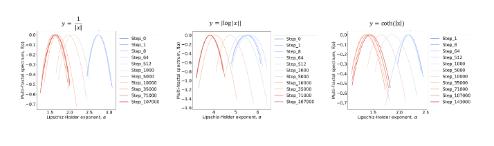
Figure 11: Different choices of weight transfer function in pythia 1B model.

C.1.2 Different Task

The analysis results for different training epochs on a Computer Vision (CV) Task using the Diffusion Model are depicted in Figure 12 (Left). On the right, analysis outcomes for a Large Language Model (LLM) of equivalent size (in terms of the number of parameters) are presented.

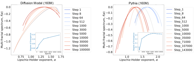
Figure 12: NeuroMFA results on stable diffusion model and the Pythia model of equivalent size.

C.1.3 Across Different Layer

In Figure 13, we showcase the analysis results considering interactions at single, double, and triple layer levels.

Figure 13: Distance across 2-3 layers in pythia 70M model.

C.1.4 Log-log Relationship Evaluation

We use $R^{2}$ (the coefficient of determination) to evaluate the log-log relationship between $N(r)$ and $r$, between $Z_{q}(r)$ and $\frac{r}{d}$ at different samples of SNIN. The detailed data can be found at Table 2.

Model	Step	R2 of $lgN(r)\sim lgr$		R2 of $lgZ_{q}(r)\sim lg\frac{r}{d}$
		Mean	Std	Mean	Std
pythia-14m	1	0.8249	0.0291	0.9125	0.0018
	2000	0.8308	0.0376	0.9160	0.0026
	5000	0.8370	0.0330	0.8943	0.0047
	10000	0.8421	0.0248	0.8613	0.0118
	143000	0.8948	0.0300	0.9763	0.0012
pythia-160m	1	0.9155	0.0594	0.9585	0.0004
	2000	0.8874	0.0419	0.9546	0.0005
	5000	0.8431	0.0195	0.9248	0.0023
	10000	0.8132	0.0168	0.8750	0.0093
	143000	0.8556	0.0391	0.9800	0.0014
pythia-1.4b	1	0.9005	0.0002	0.9279	0.0024
	2000	0.9364	0.0424	0.9287	0.0020
	5000	0.9112	0.0307	0.9700	0.0011
	10000	0.8805	0.0205	0.9336	0.0035
	143000	0.8558	0.0190	0.9489	0.0018

Table 2: Log-log relationship evaluation.

According to the statement in Appendix A.5, the log-log relationships are all above 0.7 which demonstrates strong log-log relationships between $N(r)$ and $r$, between $Z_{q}(r)$ and $\frac{r}{d}$.

C.1.5 Additional Results

We provide how the $\alpha_{0}$ and $width$ varies with the training steps in Figure 14.

Figure 14: $\alpha_{0}$ (left) and width $w$ (right) of each epoch in different models.

C.2 NeuroMFA Spectra

Figure 15 displays the averaged (with standard deviation) multifractal spectra for each model, derived from analyses across 10 SNINs under NeuroMFA.

Figure 15: Multifractal analysis spectra of 10 Synthetic Neuronal Interaction Networks (SNINs), illustrating the average spectra with shadows indicating the standard deviation. From upper left to lower right, the model sizes are 14M, 31M, 70M, 160M, 410M, 1B, 1.4B, and 2.8B respectively.

C.3 Assessment of the Degree of Emergence Across Various Datasets

Figure 20, Figure 17, Figure 19, Figure 16, Figure 18 show the result for degree of emergence under our metric.

Figure 16: Results on ARC-Easy benchmark. From upper left to lower right, the model sizes are 70M, 160M, 410M, 1B, 1.4B, and 2.8B respectively.

Figure 17: Results on WSC benchmark. From upper left to lower right, the model sizes are 70M, 160M, 410M, 1B, 1.4B, and 2.8B respectively.

Figure 18: Results on SciQ benchmark. From upper left to lower right, the model sizes are 70M, 160M, 410M, 1B, 1.4B, and 2.8B respectively.

Figure 19: Results on ARC-Challenge benchmark. From upper left to lower right, the model sizes are 70M, 160M, 410M, 1B, 1.4B, and 2.8B respectively.

Figure 20: Results on LogiQA benchmark. From upper left to lower right, the model sizes are 70M, 160M, 410M, 1B, 1.4B, and 2.8B respectively.

C.4 More Results for Weight Distribution

Figure 21, Figure 22 and Figure 23 provide more results on different scales of models.

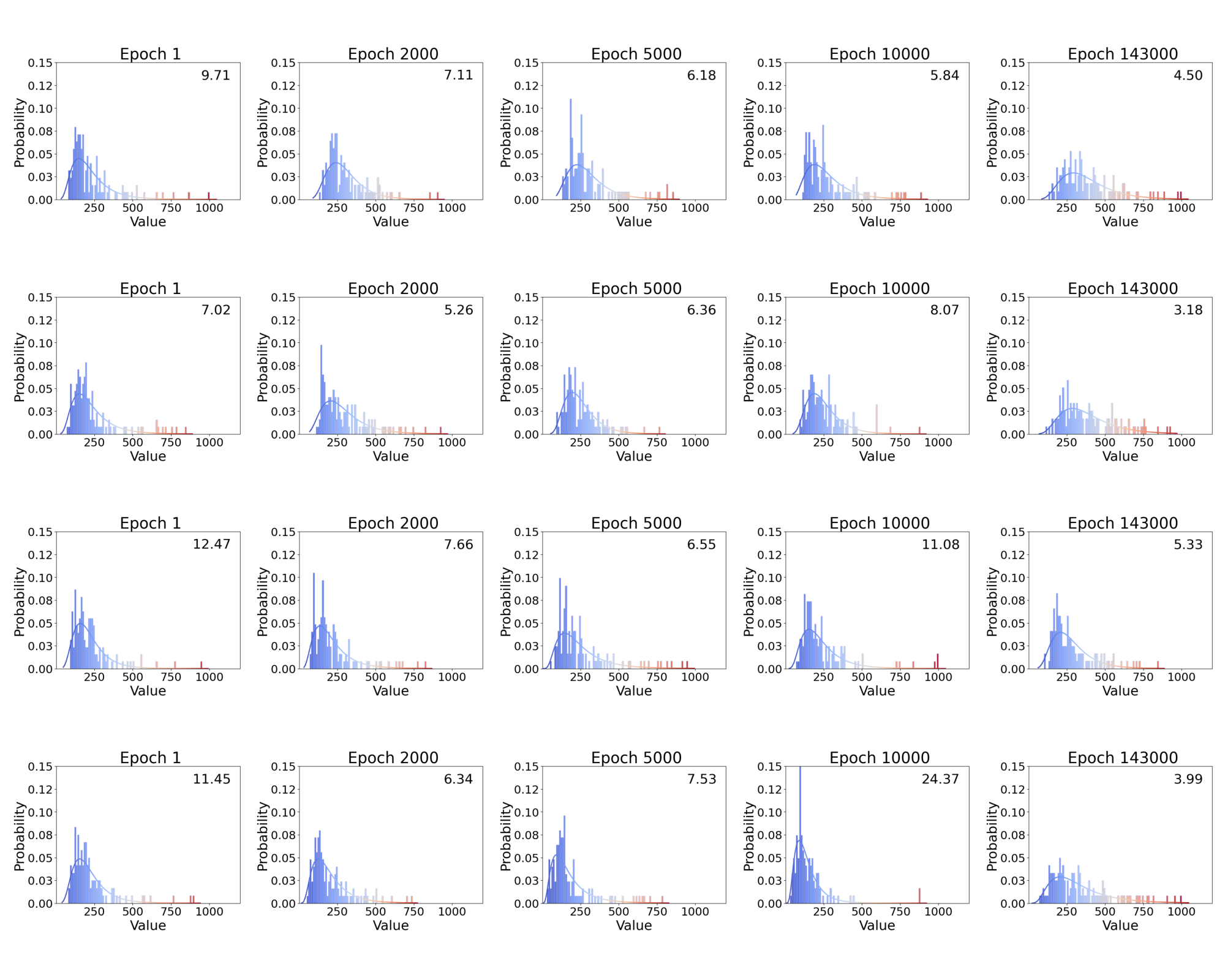
Figure 21: The distributions of average weighted degree for 14M model of different sizes in different layers during the training process.

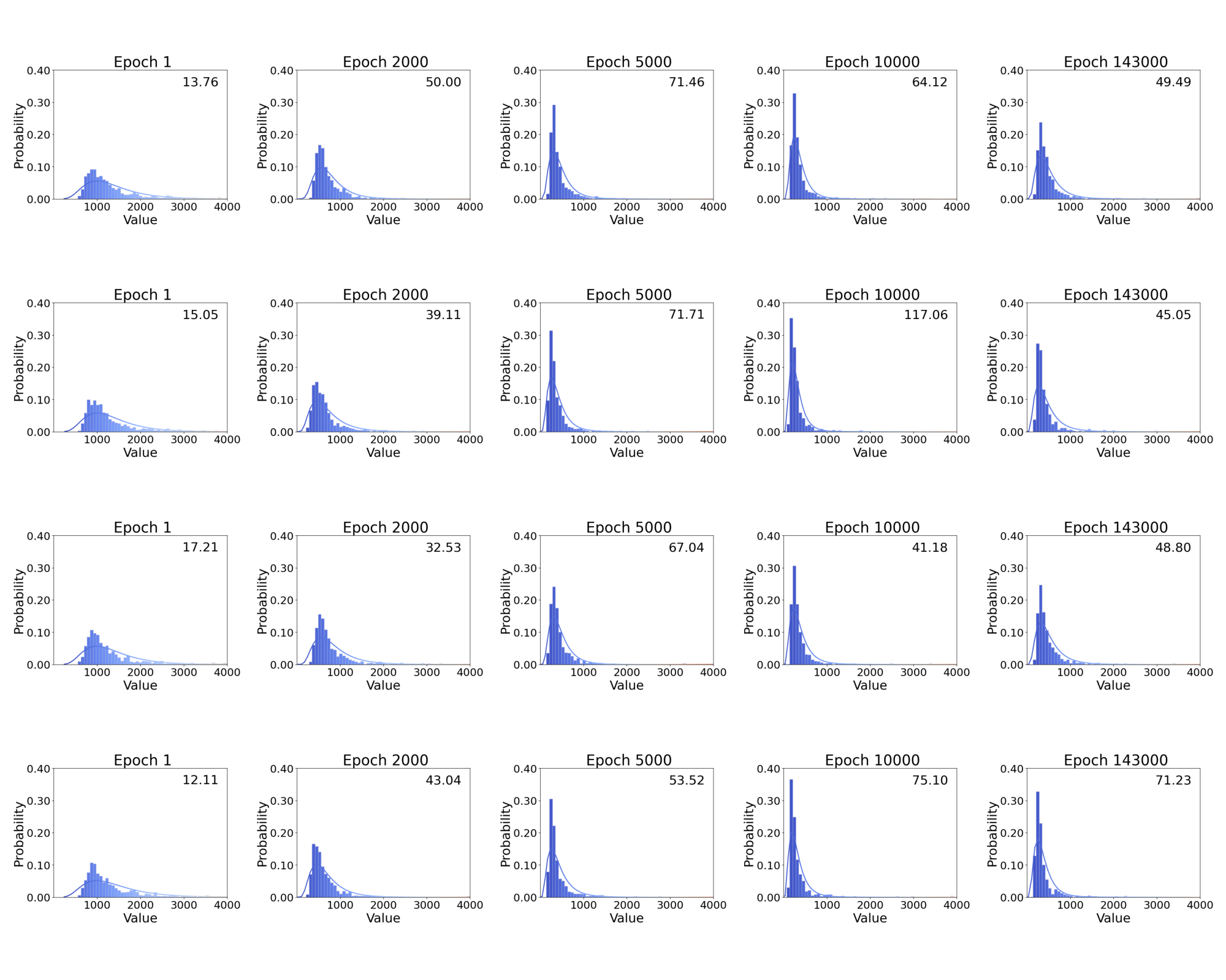
Figure 22: The distributions of average weighted degree for 160M model of different sizes in different layers during the training process.

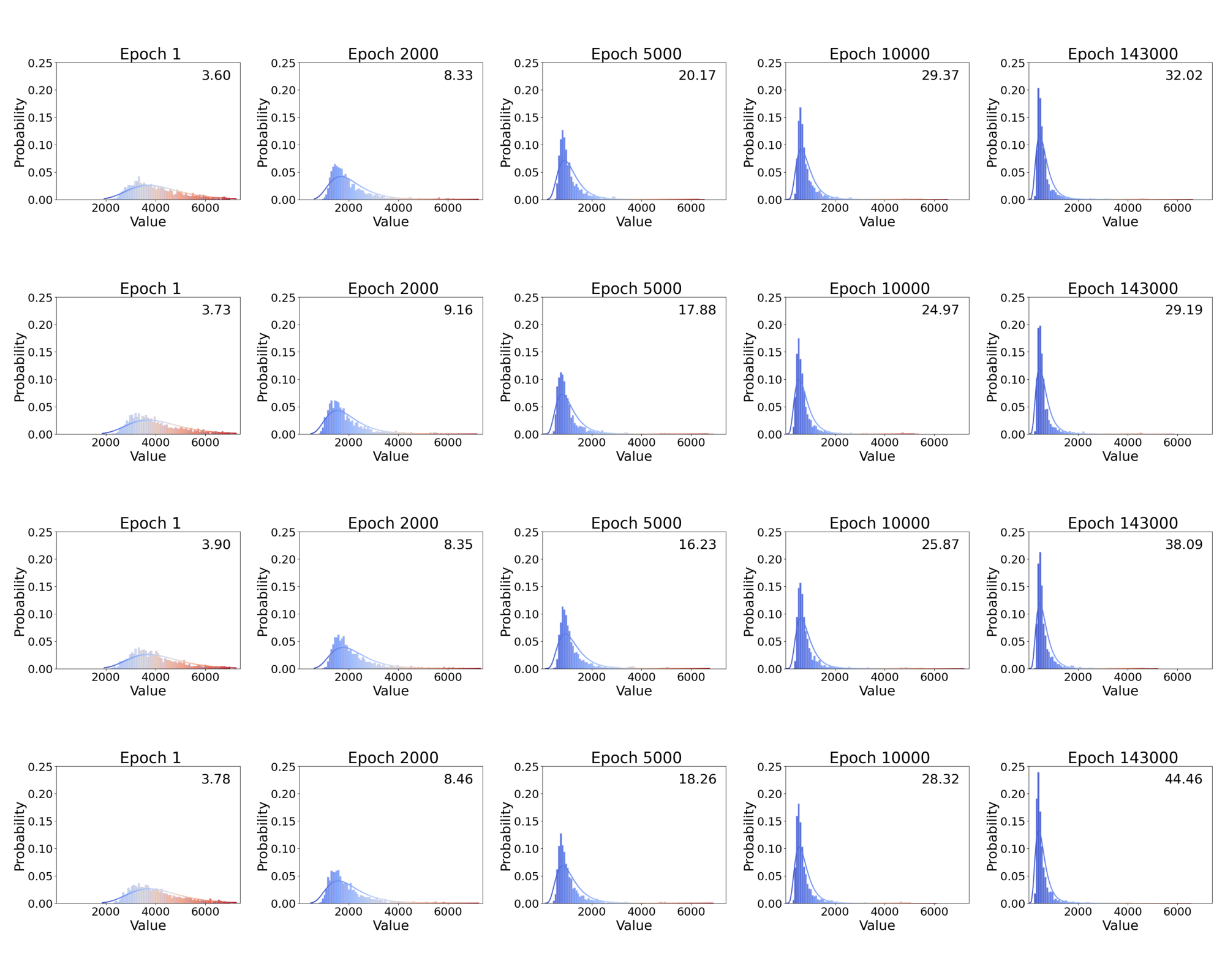
Figure 23: The distributions of average weighted degree for 1.4B model of different sizes in different layers during the training process.

Appendix D Implementation Details

The source code is available at https://anonymous.4open.science/r/Neuron_LLM-8738. Here we provide the hyper-parameters we used to produce our experiments in Table 3.

Model Name	Blocks	Model Dim	Heads	Sample1 ( x 10)		Sample2 ( x 10)		Sample3 ( x 10)
				Nodes Per Layer	Total Nodes	Nodes Per Layer	Total Nodes	Nodes Per Layer	Total Nodes
Pythia-14M	6	128	8	128	5504	64	2752	32	1376
Pythia-31M	6	256	8	128	5504	64	2752	32	1376
Pythia-70M-deduped	6	512	8	128	5504	64	2752	32	1376
Pythia-160M-deduped	12	768	12	128	10880	64	5440	32	2720
Pythia-410M-deduped	24	1024	16	128	21632	64	5440	32	2720
Pythia-1B-deduped	16	2048	8	128	14464	64	7232	32	3616
Pythia-1.4B-deduped	24	2048	16	128	21632	64	10816	32	5408
Pythia-2.8B-deduped	32	2560	32	128	28800	64	14400	32	7200

Table 3: SNIN sample parameters.

References

- tur (2022) Turing patterns, 70 years later. Nature Computational Science, 2(8):463–464, Aug 2022. ISSN 2662-8457. doi: 10.1038/s43588-022-00306-0. URL https://doi.org/10.1038/s43588-022-00306-0.
- Andonian et al. (2023) Andonian, A., Anthony, Q., Biderman, S., Black, S., Gali, P., Gao, L., Hallahan, E., Levy-Kramer, J., Leahy, C., Nestler, L., Parker, K., Pieler, M., Phang, J., Purohit, S., Schoelkopf, H., Stander, D., Songz, T., Tigges, C., Thérien, B., Wang, P., and Weinbach, S. GPT-NeoX: Large Scale Autoregressive Language Modeling in PyTorch, 9 2023. URL https://www.github.com/eleutherai/gpt-neox.
- Ay et al. (2007) Ay, N., Flack, J., and Krakauer, D. C. Robustness and complexity co-constructed in multimodal signalling networks. Philosophical Transactions of the Royal Society B: Biological Sciences, 362(1479):441–447, 2007.
- Barabási & Bonabeau (2003) Barabási, A.-L. and Bonabeau, E. Scale-free networks. Scientific american, 288(5):60–69, 2003.
- Belrose et al. (2023) Belrose, N., Furman, Z., Smith, L., Halawi, D., Ostrovsky, I., McKinney, L., Biderman, S., and Steinhardt, J. Eliciting latent predictions from transformers with the tuned lens. arXiv preprint arXiv:2303.08112, 2023.
- Biderman et al. (2023) Biderman, S., Schoelkopf, H., Anthony, Q. G., Bradley, H., O’Brien, K., Hallahan, E., Khan, M. A., Purohit, S., Prashanth, U. S., Raff, E., et al. Pythia: A suite for analyzing large language models across training and scaling. In International Conference on Machine Learning, pp. 2397–2430. PMLR, 2023.
- Bisk et al. (2020) Bisk, Y., Zellers, R., Gao, J., Choi, Y., et al. Piqa: Reasoning about physical commonsense in natural language. In Proceedings of the AAAI conference on artificial intelligence, volume 34, pp. 7432–7439, 2020.
- Black et al. (2022) Black, S., Biderman, S., Hallahan, E., Anthony, Q., Gao, L., Golding, L., He, H., Leahy, C., McDonell, K., Phang, J., et al. Gpt-neox-20b: An open-source autoregressive language model. arXiv preprint arXiv:2204.06745, 2022.
- Broido & Clauset (2019) Broido, A. D. and Clauset, A. Scale-free networks are rare. Nature communications, 10(1):1017, 2019.
- Brown et al. (2020) Brown, T., Mann, B., Ryder, N., Subbiah, M., Kaplan, J. D., Dhariwal, P., Neelakantan, A., Shyam, P., Sastry, G., Askell, A., et al. Language models are few-shot learners. Advances in neural information processing systems, 33:1877–1901, 2020.
- Bubeck et al. (2023) Bubeck, S., Chandrasekaran, V., Eldan, R., Gehrke, J., Horvitz, E., Kamar, E., Lee, P., Lee, Y. T., Li, Y., Lundberg, S., et al. Sparks of artificial general intelligence: Early experiments with gpt-4. arXiv preprint arXiv:2303.12712, 2023.
- Chan et al. (2023) Chan, C., Cheng, J., Wang, W., Jiang, Y., Fang, T., Liu, X., and Song, Y. Chatgpt evaluation on sentence level relations: A focus on temporal, causal, and discourse relations. arXiv preprint arXiv:2304.14827, 2023.
- Chowdhery et al. (2022) Chowdhery, A., Narang, S., Devlin, J., Bosma, M., Mishra, G., Roberts, A., Barham, P., Chung, H. W., Sutton, C., Gehrmann, S., Schuh, P., Shi, K., Tsvyashchenko, S., Maynez, J., Rao, A., Barnes, P., Tay, Y., Shazeer, N., Prabhakaran, V., Reif, E., Du, N., Hutchinson, B., Pope, R., Bradbury, J., Austin, J., Isard, M., Gur-Ari, G., Yin, P., Duke, T., Levskaya, A., Ghemawat, S., Dev, S., Michalewski, H., Garcia, X., Misra, V., Robinson, K., Fedus, L., Zhou, D., Ippolito, D., Luan, D., Lim, H., Zoph, B., Spiridonov, A., Sepassi, R., Dohan, D., Agrawal, S., Omernick, M., Dai, A. M., Pillai, T. S., Pellat, M., Lewkowycz, A., Moreira, E., Child, R., Polozov, O., Lee, K., Zhou, Z., Wang, X., Saeta, B., Diaz, M., Firat, O., Catasta, M., Wei, J., Meier-Hellstern, K., Eck, D., Dean, J., Petrov, S., and Fiedel, N. Palm: Scaling language modeling with pathways, 2022.
- Chowdhery et al. (2023) Chowdhery, A., Narang, S., Devlin, J., Bosma, M., Mishra, G., Roberts, A., Barham, P., Chung, H. W., Sutton, C., Gehrmann, S., et al. Palm: Scaling language modeling with pathways. Journal of Machine Learning Research, 24(240):1–113, 2023.
- Clark et al. (2018) Clark, P., Cowhey, I., Etzioni, O., Khot, T., Sabharwal, A., Schoenick, C., and Tafjord, O. Think you have solved question answering? try arc, the ai2 reasoning challenge. arXiv preprint arXiv:1803.05457, 2018.
- Correia (2006) Correia, L. Self-organisation: a case for embodiment. In Proceedings of the evolution of complexity workshop at artificial life X: the 10th international conference on the simulation and synthesis of living systems, pp. 111–116, 2006.
- Crutchfield (1994) Crutchfield, J. P. The calculi of emergence: computation, dynamics and induction. Physica D: Nonlinear Phenomena, 75(1-3):11–54, 1994.
- Dao et al. (2022) Dao, T., Fu, D., Ermon, S., Rudra, A., and Ré, C. Flashattention: Fast and memory-efficient exact attention with io-awareness. Advances in Neural Information Processing Systems, 35:16344–16359, 2022.
- Devlin et al. (2018) Devlin, J., Chang, M.-W., Lee, K., and Toutanova, K. Bert: Pre-training of deep bidirectional transformers for language understanding. arXiv preprint arXiv:1810.04805, 2018.
- Ding et al. (2023) Ding, N., Qin, Y., Yang, G., Wei, F., Yang, Z., Su, Y., Hu, S., Chen, Y., Chan, C.-M., Chen, W., et al. Parameter-efficient fine-tuning of large-scale pre-trained language models. Nature Machine Intelligence, 5(3):220–235, 2023.
- Epstein et al. (2006) Epstein, I. R., Pojman, J. A., and Steinbock, O. Introduction: Self-organization in nonequilibrium chemical systems. Chaos: An Interdisciplinary Journal of Nonlinear Science, 16(3), 2006.
- Evans & Saramäki (2005) Evans, T. and Saramäki, J. Scale-free networks from self-organization. Physical Review E, 72(2):026138, 2005.
- Evertsz & Mandelbrot (1992) Evertsz, C. J. and Mandelbrot, B. B. Multifractal measures. Chaos and fractals, 1992:921–953, 1992.
- Fu et al. (2023) Fu, Y., Peng, H., Ou, L., Sabharwal, A., and Khot, T. Specializing smaller language models towards multi-step reasoning. International Conference on Machine Learning, 2023.
- Furuya & Yakubo (2011) Furuya, S. and Yakubo, K. Multifractality of complex networks. Physical Review E, 84(3):036118, 2011.
- Gaur & Saunshi (2023) Gaur, V. and Saunshi, N. Reasoning in large language models through symbolic math word problems. arXiv preprint arXiv:2308.01906, 2023.
- Goldstein (1999) Goldstein, J. Emergence as a construct: History and issues. Emergence, 1(1):49–72, 1999.
- Gurnee et al. (2024) Gurnee, W., Horsley, T., Guo, Z. C., Kheirkhah, T. R., Sun, Q., Hathaway, W., Nanda, N., and Bertsimas, D. Universal neurons in gpt2 language models. arXiv preprint arXiv:2401.12181, 2024.
- He et al. (2020) He, P., Liu, X., Gao, J., and Chen, W. Deberta: Decoding-enhanced bert with disentangled attention. arXiv preprint arXiv:2006.03654, 2020.
- Hendrycks et al. (2020) Hendrycks, D., Burns, C., Basart, S., Zou, A., Mazeika, M., Song, D., and Steinhardt, J. Measuring massive multitask language understanding. arXiv preprint arXiv:2009.03300, 2020.
- Hu et al. (2023a) Hu, S., Liu, X., Han, X., Zhang, X., He, C., Zhao, W., Lin, Y., Ding, N., Ou, Z., Zeng, G., et al. Predicting emergent abilities with infinite resolution evaluation. arXiv e-prints, pp. arXiv–2310, 2023a.
- Hu et al. (2023b) Hu, S., Liu, X., Han, X., Zhang, X., He, C., Zhao, W., Lin, Y., Ding, N., Ou, Z., Zeng, G., et al. Unlock predictable scaling from emergent abilities. ICLR, 2023b.
- Jaiswal et al. (2023) Jaiswal, A., Liu, S., Chen, T., and Wang, Z. The emergence of essential sparsity in large pre-trained models: The weights that matter. arXiv preprint arXiv:2306.03805, 2023.
- Kaplan et al. (2020) Kaplan, J., McCandlish, S., Henighan, T., Brown, T. B., Chess, B., Child, R., Gray, S., Radford, A., Wu, J., and Amodei, D. Scaling laws for neural language models. arXiv preprint arXiv:2001.08361, 2020.
- Kauffman (1993) Kauffman, S. A. The origins of order: Self-organization and selection in evolution. Oxford University Press, USA, 1993.
- Kocijan et al. (2020) Kocijan, V., Lukasiewicz, T., Davis, E., Marcus, G., and Morgenstern, L. A review of winograd schema challenge datasets and approaches. arXiv preprint arXiv:2004.13831, 2020.
- Kondo & Miura (2010) Kondo, S. and Miura, T. Reaction-diffusion model as a framework for understanding biological pattern formation. science, 329(5999):1616–1620, 2010.
- Liu et al. (2020) Liu, J., Cui, L., Liu, H., Huang, D., Wang, Y., and Zhang, Y. Logiqa: A challenge dataset for machine reading comprehension with logical reasoning. arXiv preprint arXiv:2007.08124, 2020.
- Michaud et al. (2023) Michaud, E. J., Liu, Z., Girit, U., and Tegmark, M. The quantization model of neural scaling. In Thirty-seventh Conference on Neural Information Processing Systems, 2023. URL https://openreview.net/forum?id=3tbTw2ga8K.
- Paperno et al. (2016) Paperno, D., Kruszewski, G., Lazaridou, A., Pham, Q. N., Bernardi, R., Pezzelle, S., Baroni, M., Boleda, G., and Fernández, R. The lambada dataset: Word prediction requiring a broad discourse context. arXiv preprint arXiv:1606.06031, 2016.
- Park et al. (2005) Park, K., Lai, Y.-C., and Ye, N. Self-organized scale-free networks. Physical Review E, 72(2):026131, 2005.
- Raffel et al. (2020) Raffel, C., Shazeer, N., Roberts, A., Lee, K., Narang, S., Matena, M., Zhou, Y., Li, W., and Liu, P. J. Exploring the limits of transfer learning with a unified text-to-text transformer. The Journal of Machine Learning Research, 21(1):5485–5551, 2020.
- Rombach et al. (2022) Rombach, R., Blattmann, A., Lorenz, D., Esser, P., and Ommer, B. High-resolution image synthesis with latent diffusion models. In Proceedings of the IEEE/CVF conference on computer vision and pattern recognition, pp. 10684–10695, 2022.
- Sakaguchi et al. (2021) Sakaguchi, K., Bras, R. L., Bhagavatula, C., and Choi, Y. Winogrande: An adversarial winograd schema challenge at scale. Communications of the ACM, 64(9):99–106, 2021.
- Salat et al. (2017) Salat, H., Murcio, R., and Arcaute, E. Multifractal methodology. Physica A: Statistical Mechanics and its Applications, 473:467–487, 2017.
- Schaeffer et al. (2023) Schaeffer, R., Miranda, B., and Koyejo, S. Are emergent abilities of large language models a mirage? arXiv preprint arXiv:2304.15004, 2023.
- Song et al. (2005) Song, C., Havlin, S., and Makse, H. A. Self-similarity of complex networks. Nature, 433(7024):392–395, 2005.
- Song et al. (2007) Song, C., Gallos, L. K., Havlin, S., and Makse, H. A. How to calculate the fractal dimension of a complex network: the box covering algorithm. Journal of Statistical Mechanics: Theory and Experiment, 2007(03):P03006, 2007.
- Srivastava et al. (2022) Srivastava, A., Rastogi, A., Rao, A., Shoeb, A. A. M., Abid, A., Fisch, A., Brown, A. R., Santoro, A., Gupta, A., Garriga-Alonso, A., et al. Beyond the imitation game: Quantifying and extrapolating the capabilities of language models. arXiv preprint arXiv:2206.04615, 2022.
- Su et al. (2023) Su, J., Lu, Y., Pan, S., Murtadha, A., Wen, B., and Liu, Y. Roformer: Enhanced transformer with rotary position embedding, 2023.
- Wang & Komatsuzaki (2021) Wang, B. and Komatsuzaki, A. Gpt-j-6b: A 6 billion parameter autoregressive language model, 2021.
- Wei et al. (2022a) Wei, J., Tay, Y., Bommasani, R., Raffel, C., Zoph, B., Borgeaud, S., Yogatama, D., Bosma, M., Zhou, D., Metzler, D., et al. Emergent abilities of large language models. Transactions on Machine Learning Research, 2022a.
- Wei et al. (2022b) Wei, J., Wang, X., Schuurmans, D., Bosma, M., Xia, F., Chi, E., Le, Q. V., Zhou, D., et al. Chain-of-thought prompting elicits reasoning in large language models. Advances in Neural Information Processing Systems, 35:24824–24837, 2022b.
- Wei et al. (2023) Wei, J., Wei, J., Tay, Y., Tran, D., Webson, A., Lu, Y., Chen, X., Liu, H., Huang, D., Zhou, D., et al. Larger language models do in-context learning differently. arXiv preprint arXiv:2303.03846, 2023.
- Welbl et al. (2017) Welbl, J., Liu, N. F., and Gardner, M. Crowdsourcing multiple choice science questions. In Derczynski, L., Xu, W., Ritter, A., and Baldwin, T. (eds.), Proceedings of the 3rd Workshop on Noisy User-generated Text, pp. 94–106, Copenhagen, Denmark, September 2017. Association for Computational Linguistics. doi: 10.18653/v1/W17-4413. URL https://aclanthology.org/W17-4413.
- Xiao et al. (2021) Xiao, X., Chen, H., and Bogdan, P. Deciphering the generating rules and functionalities of complex networks. Scientific reports, 11(1):22964, 2021.
- Zheng et al. (2024) Zheng, C., Sun, K., Tang, D., Ma, Y., Zhang, Y., Xi, C., and Zhou, X. Ice-grt: Instruction context enhancement by generative reinforcement based transformers. arXiv preprint arXiv:2401.02072, 2024.
.tocmtappendix \etocsettagdepthmtchapternone \etocsettagdepthmtappendixsubsection