Exploiting Estimation Bias in Deep Double Q-Learning for Actor-Critic Methods

Abstract

This paper introduces innovative methods in Reinforcement Learning (RL), focusing on addressing and exploiting estimation biases in Actor-Critic methods for continuous control tasks, using Deep Double Q-Learning. We propose two novel algorithms: Expectile Delayed Deep Deterministic Policy Gradient (ExpD3) and Bias Exploiting - Twin Delayed Deep Deterministic Policy Gradient (BE-TD3). ExpD3 aims to reduce overestimation bias with a single $Q$ estimate, offering a balance between computational efficiency and performance, while BE-TD3 is designed to dynamically select the most advantageous estimation bias during training. Our extensive experiments across various continuous control tasks demonstrate the effectiveness of our approaches. We show that these algorithms can either match or surpass existing methods like TD3, particularly in environments where estimation biases significantly impact learning. The results underline the importance of bias exploitation in improving policy learning in RL.

1 Introduction

Reinforcement Learning (RL) is a tool for training of autonomous agents that can continuously adapt to a changing environment. Control of continuous action space agents (recht2019continuous_control) is one major area of RL. Popular approaches in the literature include Actor-Critic methods based on temporal difference learning (dann2014policy_temporal_diff). The current state-of-the-art employs Q-learning (watkins1992qlearning) in which Deep Learning models are used to learn a critic estimate from collected data, while the actor is optimized with policy gradient techniques (lillicrap2015ddpg; fujimoto2018td3; haarnoja2018sac). One critical issue in such methods is the overestimation bias generated by the Q-learning (thrun2014issues_funapprox; fujimoto2018td3). In (fujimoto2018td3), the authors introduced Twin Delayed Deep Deterministic Policy Gradient (TD3), a novel algorithm that has the same structure as Deep Deterministic Policy Gradient (DDPG). The algorithm exploits a strategy called Clipped Double Q-Learning (CDQ) to reduce the overestimation of a single critic function. Specifically, two Neural Networks (NNs) are trained independently from one another in order to learn the action value function following the current policy. In each learning step, the target for each state-action pair is identical for each NN, and the target is computed with Q-learning using the minimum of the two $Q$ estimates. CDQ prevents additional overestimation compared to standard Q-learning, at the price of introducing potential underestimation bias. The authors motivate the use of CDQ based on the observation that underestimated actions have much less impact on policy updates than overestimated actions. Other contributions from (fujimoto2018td3) include (i) the use of target networks for delayed policy updates for both the critic and the actor, which improves learning stability; (ii) regularization of the $Q$ function estimates with Target Policy Smoothing, implementing the intuitive idea that similar actions should be evaluated similarly. According to (lan2019maxmin_qlearning), in the context of discrete action spaces, the impact of underestimation may be more problematic than overestimation, depending on the specific environment and task that the agent is dealing with. In the case of continuous action spaces, underestimation could potentially lead the agent to adopt overly cautious actions, thus slowing the learning process. Recent works have tackled the problem of reducing estimation biases by proposing novel strategies, many of which exploit an ensemble of value function estimates. The main idea behind these works, which we discuss in Section 2, consists in trying to reduce the effect of the two estimation biases. Instead, in this work, motivated by numerical results showing that the overestimation bias can lead to higher performance in some circumstances, we discuss how the two biases can be exploited depending on the environment the agent is interacting with.
In this paper, we propose an alternative to TD3 that reduces overestimation with a single $Q$ estimate. This algorithm, which we call Expectile Delayed Deep Deterministic Policy Gradient (ExpD3), has computational costs similar to DDPG and performance comparable to TD3 in most cases. Potentially, it allows for more control over the estimation bias with respect to the CDQ approach. Our contributions extend inlcuding evidence that an overestimation bias is not always worse than an underestimation bias, leading to the insight that the environment dictates which bias performs better. To leverage estimation biases, we propose modifications to the TD3 algorithm. Specifically, we introduce a decision layer on top of the algorithm, formulating the choice of bias as a dual-armed bandit problem. This results in the Bias Exploiting - Twin Delayed Deep Deterministic Policy Gradient (BE-TD3) algorithm. Our results suggest that BE-TD3 is able to select the most useful estimation bias during the episodes, yielding better policies than TD3, while adding no additional computational burden. Furthermore, we explore alternative strategies for computing the policy gradient in BE-TD3, diverging from the one originally proposed in (fujimoto2018td3). Our results show that using this richer estimation in the actor updates in some cases can help stabilize learning or allow convergence to higher rewards in environments where TD3 struggled originally.

The paper is structured as follows: In Section 2, we discuss recent contributions that are relevant to the scope of this paper, while in Section 3, we briefly review the required theoretical background. Section 4 discusses overestimation and underestimation in CDQ and introduces ExpD3. In Section 5 we show through an ablation study that the introduction of an overestimation bias in CDQ can improve policy learning in some environments, leading to the development of BE-TD3. In LABEL:sec:actor we consider alternative policy gradient updates in BE-TD3. LABEL:sec:conclusions concludes the paper by briefly discussing some potential future lines of contributions.
To benchmark and compare the algorithms, we use a selection of Mujoco (mujoco) robotics environments from the OpenAI Gym suite (OpenAI_gym).

2 Related work

Estimation bias in Value function approximation is an issue that has been addressed in several papers. Q-learning in discrete action space has been shown to suffer from overestimation bias (thrun2014issues_funapprox). (hasselt2010double_qlearning) presents Double Q-learning as the first possible solution. More recently, Maxmin Q-learning (lan2019maxmin_qlearning) has shown that the use of an ensemble with more than two $Q$ estimates can further reduce this bias and improve Q-learning performances. Recent publications regarding control in continuous action spaces address both the underestimation and overestimation bias in Q-learning with the ensembling of $Q$ function estimates (kuznetsov2020controlling_overest; chen2020randomized; wei2022controlling; li2023realistic). In (kuznetsov2020controlling_overest), the authors present Truncated Quantile Critics (TQC) which extends Soft Actor-Critic (haarnoja2018sac) (SAC) using an ensemble of 5 critic estimates to yield a distributional representation of a critic and truncation of the critics’ predictions in the critic updates to reduce overestimation bias. TQC also introduces the concept of using the information from multiple Qs in the actor update. Indeed in TQC the actor is updated by optimizing with respect to a sampling of the mean of the ensemble of Qs. In (chen2020randomized), the authors present Randomized Ensembled Double Q-learning (REDQ), which shares a similar structure to TQC, but exploits a larger ensemble with 10 networks and doesn’t resort to sampling. In REDQ, the critic estimates are updated multiple times for each step in the environment, 20 times in the presented results. In (wei2022controlling), the authors present Quasi-Median Q-learning (QMQ), which uses 4 $Q$ estimates and exploits the quasi-median operator to compute the targets for the critic updates. The authors justify the quasi-median, stating that it is a trade-off between overestimation and underestimation. Instead, the policy gradient is computed with respect to the mean of the Qs. In (li2023realistic), the authors propose Realistic Actor-Critic (RAC), an algorithm that targets a balance between value overestimation and underestimation, using an ensemble of 10 $Q$ networks. At each step in the environment, the ensemble of $Q$ functions is updated 20 times with targets computed using the mean of the $Q$s minus one standard deviation, while the actor is updated one time by maximizing the mean of the $Q$ functions. In (li2023realistic), the aforementioned ensemble method is applied on top of both TD3 and SAC, as both methods achieve state-of-the-art performance and sample efficiency comparable to a Model-Based RL approach (janner2019mbpo).

Remark 2.1.

The majority of contributions discussed in this section enhance TD3 or SAC by employing large ensembles of $Q$ Networks in the critic or by performing multiple steps of training at each time step, thereby introducing extra computational complexity. In contrast, our work concentrates on enhancing Clipped Double Q-learning by leveraging estimation bias, without imposing any additional computational burden.

3 Background

Reinforcement Learning can be modeled as a Markov Decision Process (MDP), defined by the tuple $(\mathcal{S},\mathcal{A},\mathcal{P},R,\gamma)$. $\mathcal{S}$ and $\mathcal{A}$ are the state space and the action space, respectively. Both $\mathcal{S}$ and $\mathcal{A}$ are continuous, thus the transition density function, $\mathcal{P}$ is continuous as well and formalized as $\mathcal{P}:\mathcal{S}\times\mathcal{A}\times\mathcal{S}\rightarrow[0,\infty)$. $R:\mathcal{S}\times\mathcal{A}\times\mathcal{S}\rightarrow\mathbb{R}$ is the random variable describing the reward function, and $\gamma\in[0,1]$ is the discount factor. A policy $\mu$ at each time-step $t$ is a function that maps from the current state $s_{t}\in\mathcal{S}$ to an action $a_{t}\in\mathcal{A}$ with respect to the conditional distribution $\mu(a_{t}|s_{t})$. In our case, such policy is parameterized by parameters $\phi$, thus $\mu_{\phi}(a_{t}|s_{t})$ will be a Neural Network.
Reinforcement Learning is concerned with finding the policy that maximizes the expected discounted sum of rewards $R_{0}=\mathbb{E_{\mu_{\phi}}}\left[\sum_{t=0}^{\infty}\gamma^{t}r_{t}\right]$ of a specific MDP. To do so, it defines two main tools, the value function $V$ and the action-value function $Q$:

$$V^{\mu}(s) =\mathbb{E_{\mu}}\left[R_{t}|S_{t}=s\right]$$

$$Q^{\mu}(s,a) =\mathbb{E_{\mu}}\left[R_{t}|S_{t}=s,A_{t}=a\right]$$

3.1 Deterministic Policy Gradient

The definition of the $Q$ function allows for a recursive definition as follows:

$$Q^{\mu}(s,a)=\mathbb{E_{\mu}}\left[r(s,a)+\gamma\mathbb{E}[Q^{\mu}(s^{\prime},a^{\prime})]\right]$$ (1)

A famous algorithm, Q-learning, assumes that the policy at time $t+1$ is the optimal policy, thus the action selected is the one with the highest expected return, leading to a new definition of the $Q$ function:

$$Q^{\mu}(s,a)=\mathbb{E}\left[r(s,a)+\gamma\max_{a}Q^{\mu}(s^{\prime},a)\right]$$ (2)

This reformulation is now dependent only on the environment and thus is off-policy. If we model the greedy policy as a neural network $\mu$ parameterized by $\phi$, the final formulation becomes the following:

$$Q^{\mu}(s,a)=\mathbb{E}\left[r(s,a)+\gamma Q^{\mu}(s^{\prime},\mu_{\phi}(s^{\prime}))\right]$$ (3)

The DPG algorithm (silver2014deterministic_policy_grad) uses this definition to derive an update equation for the policy given a differentiable model $Q_{\theta}$ via the following equation.

$$\nabla J(\phi) \approx\nabla_{\phi}[Q_{\theta}(s,a)|_{s=s_{t},a=\mu_{\phi}(s)}]$$

$$=\nabla_{a}[Q_{\theta}(s,a)|_{s=s_{t},a=\mu_{\phi}(s)}]\nabla_{\phi}\mu_{\phi}(s)|_{s=s_{t}}$$

3.2 TD3

TD3 (fujimoto2018td3) is an improvement over DDPG that tries to address mainly the overestimation bias, and introduces three new main components: a double $Q$ estimation, a smoothing of the target for Q-learning, and a slow update.
The authors use the double $Q$ estimation in order to address the overestimation bias by changing the target of Q-learning to a conservative one.

$$y=r+\gamma\text{min}_{i=1,2}Q_{\theta^{\prime}_{i}}(s^{\prime},a^{\prime}),a^{\prime}\sim\mu_{\phi^{\prime}}(s^{\prime})$$ (4)

where $Q_{\theta^{\prime}_{i}}$ and $\mu_{\phi^{\prime}}$ are two Exponential Moving Averages (EMA) of the actual current neural network, updated at every update step via a linear combination of the EMA and the current solution:

$$\phi^{\prime}_{new}=\alpha\phi+(1-\alpha)\phi^{\prime},\alpha\in(0,1]$$

$$\theta^{\prime}_{new}=\beta\theta+(1-\beta)\theta^{\prime},\beta\in(0,1]$$

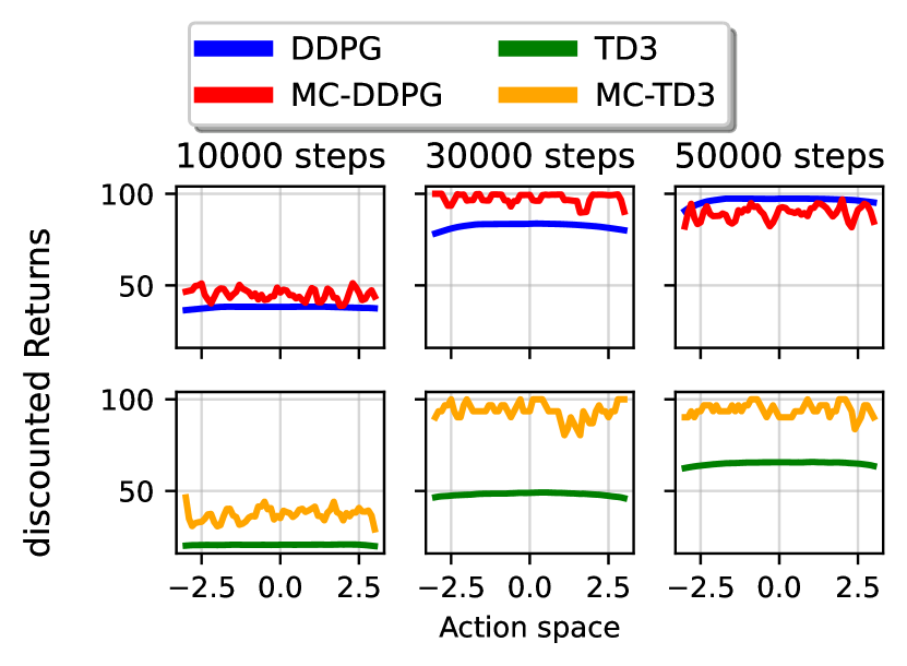
(a)

Figure 1: Q-function estimated with Monte Carlo and the critics of DDPG and TD3 in InvertedPendulum env. An optimal policy in this environment chooses actions whose discounted Return is equal to 100. For TD3, we plot the minimum between the two estimates for each action.

4 Overestimation and Underestimation in Q-Learning

When dealing with discrete action spaces, the Value function can be optimized with Q-learning with the greedy target $y=r+\text{ max}_{a^{\prime}}Q(s^{\prime},a^{\prime})$. However, in (thrun2014issues_funapprox), it has been proven that if this target has an error, then the maximum over the value biased by this error will be greater than the true maximum in expectation. Consequently, even when errors initially have mean zero, they probably lead to consistent overestimation biases in the updates of values, which are then carried through the Bellman equation. In (fujimoto2018td3), the authors have shown both analytically and experimentally that this overestimation bias is also present in actor-critic methods. While the overestimation may seem minor with each value update, the authors express two concerns. First, if not addressed, the overestimation could accumulate into a more substantial bias over numerous updates. Second, an imprecise value estimate has the potential to result in suboptimal policy updates. This poses a significant issue, as it initiates a feedback loop where suboptimal actions, favored by the inaccurate critic, can be reinforced in subsequent policy updates. For these reasons, CDQ was introduced in (fujimoto2018td3) in the algorithm TD3, showing significant improvements with respect to previous state-of-the-art, i.e. DDPG. However, CDQ has two main drawbacks: (i) it introduces an uncontrollable underestimation bias in the critic, and (ii), memory and computation consumption are doubled in the critic estimate due to the introduction of a second $Q$ network. In the rest of this section, we show experimentally the effects of the uncontrolled underestimation bias in TD3 in terms of Value function approximation. Secondly, we propose an extension to DDPG for the control of the overestimation bias without the introduction of a second $Q$ network.

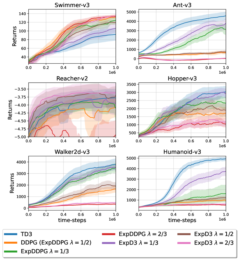
Figure 2: Training progress curves for continuous control tasks in OpenAI Gym, showing the effect of different choices of $\lambda$ in ExpD3 and ExpDDPG. Plots and shaded areas indicate mean and half a standard deviation, respectively from evaluation across 10 trials. Benchmarks were performed on 10 random seeds for simulator and network initializations. Curves are smoothed uniformly for visual clarity.

4.1 DDPG vs TD3 in Value Approximation

While TD3 may exhibit noticeable outcomes, it cannot assure compensation for the overestimation inherent in Q-learning, as discussed in both (wei2022controlling) and (li2023realistic). This effect is particularly evident when the dimension of the action space is low, we illustrate this effect in the experiment of Figure 1. In this experiment, we run DDPG and TD3 on the InvertedPendulum environment of Mujoco with the same settings of (fujimoto2018td3) for a maximum number of 50K steps, and we freeze both the critic and the actor parameters at every 10K steps. In each row of Figure 1, we plot the average over 10 uniformly sampled initial states of the critics trained in DDPG and TD3 for an increasing number of steps in the environment. The critics are compared with a Monte Carlo estimate of the discounted Return over the action space obtained starting from the same sampled initial states with the respective actors of DDPG and TD3. Both DDPG and TD3 are able to train an optimal policy for this environment. In Figure 1, we can see that in the final steps, DDPG is overestimating each possible action, while TD3 is underestimating each action at each step. The absolute errors of function approximation are higher in TD3’s critic.

4.2 Tackling Overestimation with a single $Q$ estimate

TD3 applies CDQ in the critic updates in order to favor underestimation over overestimation.
While it is theoretically sound, taking the min between the two estimates leaves very little room for adjusting this bias in case we have evidence that it’s hurting the performances.
For this reason, we explore a method that allows more control over a possible underestimation bias to compensate for the overestimation induced by Q-learning, with a single $Q$ function estimate, thus making it computationally cheaper than CDQ.
Specifically, we propose to change the CDQ mechanism with an Expectile Regression Loss for a single $Q$ function.
The $\lambda\in(0,1)$ Expectile Regression is the solution of an asymmetric loss, in particular the Mean Squared Loss, that relaxes one of the two sides of the graph.

$$L^{\lambda}(f_{\theta}(x),y)=\frac{1}{Z}\begin{cases}(1-\lambda)(y-f_{\theta}(x))^{2}&\text{if $f_{\theta}(x)>y$,}\\ \lambda(y-f_{\theta}(x))^{2}&\text{otherwise}\end{cases}$$ (5)

with $Z=\max(\lambda,1-\lambda)$.
In this formalization, $\lambda$ controls the overestimation-underestimation bias, namely:

1. $\lambda=\frac{1}{2}$ reverts MSE;

2. $\lambda>\frac{1}{2}$ favors overestimation errors;

3. $\lambda<\frac{1}{2}$ favors underestimation errors.

Such loss then leads to the following objective for the DDPG algorithm for the optimization of the $Q$ function:

$$L(\theta)=\mathbb{E}[L^{\lambda}(Q_{\theta}(s,a),r(s,a)+\gamma Q_{\theta^{\prime}}(s^{\prime},\mu_{\phi^{\prime}}(s^{\prime})))]$$ (6)

Similar approaches have already been used in other areas of Deep Reinforcement Learning to tackle overestimation (kostrikov2021offline). However, differently from other methods, we add a normalizing constant $Z$ in front of the equation in order to have a fair comparison between algorithms. From an optimization standpoint, it’s equivalent to a change in the step size of the optimization. Indeed, thanks to $Z$, the type of error we prefer to penalize, the one with the highest coefficient, has exactly $1$ as a constant in front, leading to an update that is equivalent to the original method. For the other type of error, on the other hand, the loss is multiplied by a constant $<1$, leading to a lower step size. This way, we can guarantee that the improvements shown by this proposal are due to the effectiveness of the loss and not by bigger step sizes induced by constants in the loss.
Based on this new objective, we propose a new algorithm that we will call Expectile Delayed Deep Deterministic Policy Gradient (ExpD3). ExpD3 corresponds exactly to TD3 without the CDQ mechanism, which is replaced by the new expectile loss. For this reason, ExpD3 has three main differences with respect to DDPG: the expectile loss, the target smoothing, and the delayed policy update. Since this method also includes the delayed policy update mechanism proposed in (fujimoto2018td3), the final algorithm is even computationally cheaper than the original DDPG, as it updates the actor-network only once every $d$ critic updates. In order to have a better understanding of the improvement introduced by the new loss, we also augment the DDPG algorithm with it, calling it ExpDDPG. Note that when setting $\lambda=\frac{1}{2}$, ExpDDPG reverts to DDPG, and ExpD3 to TD3 without the CDQ mechanism. In Figure 2, we report the results on multiple OpenAI Gym environments, showing the effect of different choices of $\lambda$. Specifically, it’s well known that Humanoid is the most challenging environment, and even many state-of-the-art methods struggle to match the performances of TD3 on it without having to use expensive tricks, such as multiple updates per step or by introducing additional Q-function estimators, Additionally, Humanoid is the only environment where the proposed method under-performs TD3. For the rest of the environments, at least one version of ExpD3 either matches the performances of TD3 or even surpasses it, specifically in another notoriously challenging environment, Swimmer. In Swimmer, the underestimation hinders the performances significantly, and even DDPG outperforms TD3. Furthermore, it can clearly be seen that the performances are inversely proportional to $\lambda$, showing strong evidence of how any underestimation in this environment heavily hinders learning. Finally, it must be noted that the expectile loss improves DDPG without it except for Swimmer. Notably, in Humanoid, the hardest environment, only thanks to the expectile loss we can get any form of result.

5 Estimation bias in Critic updates with Deep Double Q-Learning

In this section, we investigate the effects of estimation bias on the critic updates of TD3. We present an ablation study obtained by changing the computation of targets for Clipped Double Q-learning. Namely, in TD3 the targets are computed as in Equation 4. Here we consider 3 alternative strategies:
TD3_MaxCritic (TD3_MC):

$$y=r+\gamma\text{max}_{i=1,2}Q_{\theta_{i}^{\prime}}(s^{\prime},a^{\prime}),$$ (7)

with this update, we compute the Q-learning targets using the maximum value between the $Q$ Networks. This increases the overestimation bias and adds no underestimation. This is the exact opposite of TD3’s target update.
TD3_AverageCritic (TD3_AC):

$$y=r+\gamma\frac{1}{2}\left(Q_{\theta_{1}^{\prime}}(s^{\prime},a^{\prime})+Q_{\theta_{2}^{\prime}}(s^{\prime},a^{\prime})\right),$$ (8)

with this update, we compute the Q-learning targets using the mean value between the Q-networks. This update doesn’t introduce additional estimation bias, and the overestimation bias of Q-learning is possibly reduced. TD3_RandomCritic (TD3_RC):

$$y=r+\gamma\left(\beta Q_{\theta_{1}}(s^{\prime},a^{\prime})+(1-\beta)Q_{\theta_{2}}(s^{\prime},a^{\prime})\right)$$ (9)

where $\beta\in{0,1}$ is a binary mask, sampled uniformly randomly before each episode to select which network is used to compute the targets. Each of these target update strategies is applied to TD3, while the rest of the algorithm is the same as described in (fujimoto2018td3).

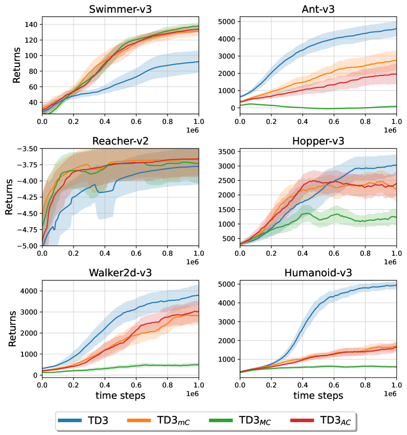
(a)

Figure 3: Training progress curves for continuous control tasks in OpenAI Gym, showing the effect of the different target computations in TD3. Plots and shaded areas indicate respectively mean and half a standard deviation from evaluation across 10 trials. Benchmarks were performed on 10 random seeds for simulator and network initializations.

This results in creating a different version of TD3 for each strategy. To evaluate the performance of each version of TD3, we benchmark on the environments from OpenAI Gym (OpenAI_gym). We report the results of a significant subset of the environments in Figure 3.

Algorithm 1 Bias Exploiting TD3

  Initialize critic $Q_{\theta_{1}},Q_{\theta_{2}}$, and actor $\mu_{\phi}$ networks

  Initialize target networks $\theta_{1}^{\prime}\leftarrow\theta_{1},\theta_{2}^{\prime}\leftarrow\theta_{2},\phi^{\prime}\leftarrow\phi$

  Initialize replay memory $\mathcal{B}$

  Initialize bandit problem: $\varepsilon_{d}$, $\alpha$, $e_{r}$

5:  $t=0$, $\varepsilon=0.9$, $Q_{b}=[0,0]$

  repeat

     $k=0$, $R=0$, $e=0$, $s\sim p(s_{0})$

     $c_{b}$ $\leftarrow$ $\varepsilon$-greedy choice from $Q_{b}$

     repeat

10:        Select action with exploration noise $a\sim\mu_{\phi^{\prime}}(s)+\omega$, $\omega\sim\mathcal{N}(0,\sigma)$ and observe $r$ and $s^{\prime}$.

        $done=s^{\prime}\text{ is terminal},R=R+r$

        Store $(s,a,r,s^{\prime})$ tuple in $\mathcal{B}$

        Sample mini-batch of $N$ tuples $(s,a,r,s^{\prime})$ from $\mathcal{B}$

        $\tilde{a}\leftarrow\mu_{\phi^{\prime}}(s^{\prime})+\omega$, $\omega\sim\text{clip}(\mathcal{N}(0,\tilde{\sigma}),-c,c)$

15:        if $c_{b}==0$ then

           $y=r+\gamma\text{min}_{i=1,2}Q_{\theta_{i}^{\prime}}(s^{\prime},\tilde{a})$ [Equation 4]

        else if $c_{b}==1$ then

           $y=r+\gamma\text{max}_{i=1,2}Q_{\theta_{i}^{\prime}}(s^{\prime},\tilde{a})$ [Equation 7]

        end if

20:        Update critics $\theta_{i}\leftarrow\text{argmin}_{\theta_{i}}\frac{1}{N}\Sigma(y-Q_{\theta_{i}}(s,a))^{2}$

        if $t$ mod $d$ then

           Update $\phi$ by deterministic policy gradient:

           $\nabla_{\phi}J(\phi)=\frac{1}{N}\Sigma\nabla_{a}Q_{\theta_{1}}(s,a)|_{a=\mu_{\phi}(s)}\nabla_{\phi}\mu_{\phi}(s)$

           Update target networks:

25:           $\theta_{i}^{\prime}\leftarrow\tau\theta_{i}+(1-\tau)\theta_{i}^{\prime}$

           $\phi^{\prime}\leftarrow\tau\phi+(1-\tau)\phi^{\prime}$

        end if

        $k=k+1$

     until not $done$ and $k<K$ and $t+k<T$

30:     $Q_{b|c_{b}}=Q_{b|c_{b}}+\alpha(R-Q_{b|c_{b}})$

     $t=t+k$, $e=e+1$

     if $e\text{ mod }e_{r}$ then $\varepsilon=0.9$

     else $\varepsilon=\varepsilon\cdot\varepsilon_{d}$

  until $t<T$

It is possible to observe that the tested algorithms share similar performance in the first steps while becoming noticeably different in the transitory steps, with very distinct final values. We can observe that in the environments Ant, Hopper, Walker, and Humanoid, TD3 reaches higher Returns than the other modifications within the available time. In these environments in particular, it is possible to notice a distinct trend: TD3 performs the best, TD3_MC performs the worst, while TD3_AC and TD3_RC both lie somewhere in the middle, with no noticeable difference between the two.
Instead, in Reacher and Swimmer, the relationship is somewhat inverted, with TD3_MC performing the best and TD3 performing the worst. These results indicate that in some environments, the additional overestimation in TD3_MC is beneficial for exploring high-rewarding actions. This could be due to environment dynamics, type of reward function, or a combination of both, as shown in (lan2019maxmin_qlearning) for discrete action spaces. The main result of this ablation study is that none of the considered update strategies performs the best among all the considered environments, including CDQ from TD3. For these reasons, we look into the idea of learning to exploit the correct estimation bias online. With correct, we refer to the bias that statistically brings the policy to higher rewards, which doesn’t necessarily mean that the value function is closer to the true $Q$. We propose Bias Exploiting - Twin Delayed Deep Deterministic Policy Gradient (BE-TD3), which extends TD3, adding a decision layer on top of the original algorithm to select which bias to use, namely Equation 4 or Equation 7. The algorithm shares the structure of DDPG and TD3, where like TD3, it trains a pair of critics and a single actor. For both the critics and actors, a target copy is maintained and slowly updated to compute the Q-learning targets. At the beginning of each episode, an $\varepsilon$-greedy policy, guided by a tabular value function $Q_{b}\in\mathbb{R}^{2}$, calculates the bias choice $c_{b}\in\{0,1\}$. In this context, $c_{b}=0$ denotes underestimation, while $c_{b}=1$ corresponds to overestimation. $Q_{b}$ is initialized to the zero vector at the initial episode, and it is updated using the undiscounted return $R$ obtained at the termination of the episode, with a fixed step size. The scalar $\varepsilon$ is initialized to 0.9, and it decays exponentially each time a decision is taken. During an episode, at each time step, we update the pair of critics with the update rule from Equation 4 if $c_{b}=0$, else with Equation 7 if instead $c_{b}=1$. In both cases, the targets are computed using target policy smoothing. The actor is updated every $d$ steps (delayed updates), with respect to $Q_{\theta_{1}}$ following the deterministic policy gradient algorithm (silver2014deterministic_policy_grad). The formulated bandit is subject to strongly changing dynamics, due to the updates of the actor. This translates to the following consideration: if a bias is preferred during the initial episodes, it might not be the best choice during the remaining interaction time. To deal with this, we reset $\varepsilon$ to its initial value for each $k_{\varepsilon}$ episodes. Namely, once every $k_{\varepsilon}$ episodes, the algorithm explores again the bias choice. In general, the $\varepsilon$ decay scheduling is an important aspect of the algorithm, as it can strongly influence performance. Alternative schedulings are discussed in the Appendix. We report the algorithm in Algorithm 1 and its benchmarks in LABEL:fig:benchmarks_BETD3. Moreover, for each environment, we plot the probability of choosing overestimation and the $\varepsilon$ scheduling over the episodes. Results are commented at the end of the next section to provide a more exhaustive outlook.