Steady-State Error Compensation for Reinforcement Learning with Quadratic Rewards
Abstract
The selection of a reward function in Reinforcement Learning (RL) has garnered significant attention because of its impact on system performance. Issues of steady-state error often manifest when quadratic reward functions are employed. Although existing solutions using absolute-value-type reward functions partially address this problem, they tend to induce substantial fluctuations in specific system states, leading to abrupt changes. In response to this challenge, this study proposes an approach that introduces an integral term. By integrating this term into quadratic-type reward functions, the RL algorithm is adeptly tuned, augmenting the system’s consideration of long-term rewards and, consequently, alleviating concerns related to steady-state errors. Through experiments and performance evaluations on the Adaptive Cruise Control (ACC) model and lane change models, we validate that the proposed method not only effectively diminishes steady-state errors but also results in smoother variations in system states.
Index Terms:
Reinforcement Learning, Reward Function, Steady-State Error, PID.I Introduction
Reinforcement learning is a data-driven, model-free approach[1]. In 2015, Mnih et al. pioneered the fusion of deep learning with reinforcement learning by introducing the Deep Reinforcement Learning (DRL) algorithm, which significantly augmented the representational capacity and generalization performance of reinforcement learning algorithms[2]. Today, this approach has extensive applications across various industries, including gaming, robotics, natural language processing, healthcare, Industry 4.0, smart grids, and beyond[3].
Optimal control theory is centered on crafting control policies to attain optimal performance for a given system based on a specific performance metric. This metric is commonly expressed as a cost or objective function, and the objective of optimal control is to discover a control policy that minimizes or maximizes this performance metric[4]. However, conventional optimization methods may encounter challenges when confronted with uncertainties and changes in dynamic environments[5]. RL serves as a bridge between traditional optimal control and adaptive control algorithms[6].
In control engineering, RL is adept at uncovering optimal control laws. Through iterative interactions with the environment, optimal control strategies can be identified without necessitating a precise system model, relying instead on a trial-and-error approach. Reinforcement Learning is conceptualized as a Markov Decision Process (MDP), where the agent (controller) observes the state of the environment, takes actions, receives rewards or penalties, and refines its policy based on this feedback. Through continual learning and optimization, reinforcement learning progressively unveils the optimal control law, empowering the system to attain optimal performance in specific tasks or goals[7]. The reward function in reinforcement learning is akin to the cost function in control theory, defining the agent’s objectives in the environment and exerting direct influence over the algorithm’s performance, convergence speed, and the nature of the optimal policy[8].
As reinforcement learning algorithms advance, reconsideration of reward function design becomes imperative. Booth et al. discovered that reward functions precisely aligned with actual task performance metrics often tend to be sparse[9]. Real task metrics may encode success as a reward of 1 and failure as 0. Sparse task metrics are frequently challenging to learn, leading to the common use of dense reward functions in practice. These dense reward functions are typically crafted through trial and error by experts[10]. While dense reward functions prove more efficient in exploration, they necessitate ongoing interaction with the environment for tuning, delicately balancing the relative value of each state-action pair to ultimately derive a robust reward function[11]. The output format of the reward function, the setting of parameter weights, and the specific content of reward terms all have a significant influence on the final control performance.
Engel et al. established a connection between the reward function and the ultimate control performance of closed-loop systems. Their research revealed that a reward function grounded in quadratic values could result in notable steady-state errors in the final state variables, attributed to the discounting nature of rewards in RL algorithms. Furthermore, their exploration of absolute value-based reward functions demonstrated a decrease in steady-state errors and a learning curve resembling that of quadratic rewards. However, it was noted that the learning time for absolute value-based curves significantly increased compared to quadratic rewards[12].
To guarantee the reasonable characteristics of the learned curves in reinforcement learning, we introduce the Interior-Point Optimization (IPO) method for reference. The IPO solution resides within the set of inequality constraints and closely approximates the true optimal solution. The primary contributions of this study can be summarized as follows:
This study identified that the reward function based on the absolute value still induces considerable fluctuations in specific state changes throughout the entire control process, resulting in prominent peaks. Nevertheless, the introduction of an integral term offers a dual benefit, it helps diminish the steady-state error of the square function and concurrently alleviates the peaks associated with the absolute value. The subsequent sections of this paper are as follows:
Section \@slowromancapii@ introduces the basic theory of reinforcement learning and the Deep Deterministic Policy Gradient (DDPG) algorithm. Section \@slowromancapiii@ outlines the specific method for introducing the integral term. Section \@slowromancapiv@ details the modeling of the experimental environment and conducts simulations to validate the proposed method. Section \@slowromancapv@ summarizes the entire paper.
II PRELIMINARY
II-A Reinforcement Learning
A MDP serves as the ideal mathematical model for RL[13]. In a standard RL process, it is initially assumed that the environment interacts with the agent. At each time step , the agent receives observations from the environment, takes action , causing the environment to change on the basis of the agent’s actions, and receives an immediate reward . Generally, the environment’s state is partially observable to the agent, often considering a set of historical state-action pairs as the current state. In this context, we consider reinforcement learning to be entirely observable, allowing the agent to access global information.
The agent’s actions are determined by policy . The policy is a function that expresses the probability of taking action given the input state . When a policy is deterministic, it outputs only one specific action with a probability of one at each state, whereas the probabilities of other actions are 0. In the case of a stochastic policy, it outputs a probability distribution over actions at each state, and action can be sampled on the basis of this distribution. Probability of the agent transitioning from state to the next state after taking action according to policy is defined as , representing the state transition probability with Markovian properties. In a MDP, starting from time step 0 until reaching the termination state, the sum of discounted rewards is referred to as the return.
| (1) |
Here, is the discount factor, reflecting the ratio between the future reward value and the current reward value.
Furthermore, the definition of maximizing the cumulative expected return is introduced. Considering the presence of actions in MDP, the action-value function is defined:
| (2) |
It represents the cumulative expected return when performing action in a certain state . The Bellman equation is then derived as
| (3) | ||||
It can be used for iterative solutions to obtain the action-value function . Ultimately, the core objective of reinforcement learning is to determine an optimal policy
| (4) |
It can maximize the action-value function .
II-B DDPG Algorithm
The DDPG algorithm combines concepts from deterministic policy gradient algorithms and extends the action space to continuous space, thus establishing itself as a model-free deep reinforcement learning algorithm[14]. Built upon the actor-critic framework, it employs deep neural networks to approximate both the policy network and the action-value function. Training of the policy network and value network model parameters is accomplished through stochastic gradient descent. The algorithm adopts a dual neural network architecture for both the policy and value functions, consisting of online and target networks, enhancing stability during the learning process and expediting convergence. In addition, the algorithm incorporates an experience replay mechanism, where data generated by the actor interacting with the environment is stored in an experience pool. Batch data samples are then extracted for training, similar to the experience replay mechanism in Deep Q-Network, with the aim of eliminating sample correlations and dependencies to improve convergence. The pseudocode is provided as Algorithm 1.
III method
III-A Problem Statement
The quadratic reward function of RL is defined as follows:
| (5) | |||
In this context, and is the state and action, represents the desired state value, and are weighting matrices. These matrices are used to fine-tune the relative impacts of the state, action vector, and rate of state changes on the overall cost. Among these, the rate of state changes considers factors such as comfort and safety in specific control problems. For instance, in the context of a moving car, if the acceleration change rate is too high, it will make passenger uncomfortable. In contrast to the cost function in optimal control, where the objective is to minimize a cost function, reinforcement learning strives to maximize expected returns.
Similarly, the absolute value reward function is defined as:
| (6) |
Where is the weight matrix. After determining the specific reward functions, experiments were conducted using both the square and absolute value reward functions, as illustrated in Section \@slowromancapiv@. The results clearly demonstrate that, for the square reward function, although it achieves relatively smooth control, the difference between and is larger than that for the absolute value reward function. On the other hand, the absolute value reward function, while achieving smaller steady-state errors, exhibits higher peak rates of fluctuation in the state during the control process.
To address this issue, we propose two new reward functions based on integral terms:
III-B Solution
The two reward functions presented in this study are both derived from the square reward function, chosen for its superior smoothness, which helps avoid significant peaks in the system’s variables. The fundamental concept is to mitigate the steady-state error associated with the square reward function. Analogous to the incorporation of integral terms in PID control to diminish steady-state errors in control systems, this study aggregates the system’s steady-state errors and integrates them as a novel penalty into the reinforcement learning reward function. The goal is to prompt the agent to prioritize the subtle yet persistent penalties embedded in the reward function.
Therefore, the reward function incorporating the steady-state error is defined as:
| (7) | |||
represents the accumulated error term. Through experiments, it has been observed that if the weights of the accumulated error over the entire control process are summed up, the training process becomes very slow and sometimes struggles to converge. Therefore, two methods are proposed to calculate the accumulated error term. The first method is as follows:
| (8) |
Where is used to describe the error value at time , is used to describe the accumulated error from the previous time step. The variable is defined as a threshold, and its setting depends on when the system enters a steady state. This approach does not calculate errors before the system enters a steady state; it only sums up the smaller steady-state errors after stabilization. On the one hand, it allows for the use of relatively large weight values to reduce steady-state errors, and on the other hand, it significantly improves the convergence speed of reinforcement learning.
In most cases, if the approximate time to reach steady state is unknown in advance and cannot be obtained through experimentation, the first method may fail to determine its critical value. Hence, we introduce the second method:
| (9) |
Here, is a weighting factor that can be artificially set depending on the environment. Its purpose is to reduce the weight of errors during transient changes, ensuring that the RL strategy is not excessively influenced by accumulated transient change errors, thus accelerating convergence. Therefore, should gradually increase over time steps, aligning with our increasing emphasis on steady-state errors. For example, a direct proportionality function. In this study, we use the function to represent the term:
| (10) |
is the length of an episode. The scaling of the function can be controlled by adjusting its parameters, typically denoted as .
IV Simulation
This section primarily introduces the two models applied in the experiments of this article: the ACC and lane change models, along with the design of their reward functions. Additionally, the presentation of the experimental results is discussed.
IV-A Model
IV-A1 ACC
The schematic of the ACC is shown as Fig. 1.
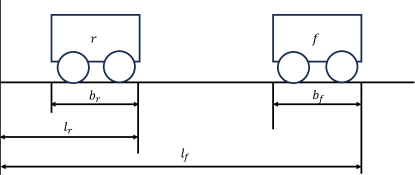
Where represents the tracked target vehicle, is the controlled vehicle is the length of the target vehicle is the length of the controlled vehicle, is the distance traveled by the controlled vehicle, and is the distance traveled by the target vehicle. The equations for the spacing and velocity errors between the target and controlled vehicles are as follows:
| (11) | ||||
Where is the standstill safety distance and is the headway time. This study adopts a first-order inertia system to approximate the vehicle motion process, leading to the following state-space equations:
| (12) | ||||
Where is the actual acceleration of the controlled vehicle, is the actual acceleration of the target vehicle, is the system output representing the desired acceleration of the controlled vehicle, and is the constant of the first-order inertia system. To minimize variables that could cause steady-state errors, this study sets , indicating that the preceding vehicle is moving at a constant speed.
For the RL in the ACC environment, the state variables are set as (), the output actions as , and the initial state is configured as (5, 5, 0).
IV-A2 Lane change
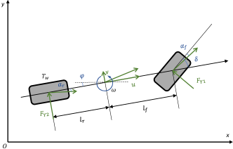
The vehicle dynamics model used for lane change in this study is illustrated in Fig. 2:
The state-space equations are as follows:
| (13) | ||||
Where and represent the distances of the vehicle along the and axes, is the angle between the vehicle body and the x-axis, is the velocity of the vehicle center of mass along the body, is the velocity of the vehicle center of mass perpendicular to the body, is the angular velocity of the vehicle body, and a stores the decision made by the vehicle in the previous time step. is the lateral force. under mild steering angle, we can assume that:
| (14) | ||||
The lane change scenario considered in this paper involves the simplest case, as depicted in Fig. 7. The controlled vehicle smoothly approaches the centerline of the second lane. Therefore, the vehicle’s acceleration is defined as 0, and the state variable is not considered during the control process. The distance of the vehicle in the y-direction from the centerline of the second lane is defined as , which serves as a measure of the steady-state error in vehicle control.
For the RL in the lane change environment, the state variables are set as (), and the output actions as . The initial state is configured as (4, 0, 30, 0, 0, 0).
IV-B Reward function
Here, only the terms corresponding to nonzero weights in the previous reward function are mentioned. Therefore, the four reward functions are defined as follows:
| (15) | |||
| (16) | |||
The PI-reward function is defined as , . and correspond to Methods 1 and 2, respectively:
| (17) |
| (18) |
The first term corresponds to the spacing error in the ACC system and the distance of the vehicle from the centerline of the second lane in the lane-changing system. The second term represents the penalty for actions in both the ACC and lane change systems, while the third term corresponds to the acceleration in the ACC system and the rate of angle change in the lane-changing system. denotes the weights, and the remaining coefficients are normalization factors. The specific values for all coefficients are provided in the Table I and Table II.
| Parameter | Values |
| Constant time gap | 1s |
| Time step | 0.1s |
| Allowed maximum control input | 2m/ |
| Allowed minimum control input | -3m/ |
| Nominal maximum gap-keeping error | 15m |
| 60m | |
| 125 | |
| 0.4 | |
| in | |
| for | 0.1 |
| for | 0.05 |
| Parameter | Values |
| Mass of the vehicle | 1470kg |
| Time step | 0.1s |
| Yaw inertia of vehicle body | 2400kg* |
| Front axle equivalent sideslip Stiffness | -100000N/rad |
| rear axle equivalent sideslip Stiffness | -100000N/rad |
| Centroid to front axle distance | 1.085m |
| Centroid to rear axle distance | 2.503m |
| Allowed maximum control input | |
| Allowed minimum control input | |
| Nominal maximum lateral error | 4m |
| Distance between two centerlines | 4m |
| 15m | |
| 0.1 | |
| 30 | |
| in | |
| for PI1 | 0.1 |
| for PI2 | 0.5 |
IV-C Result
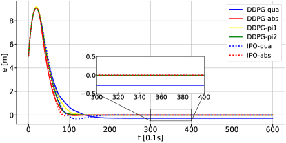
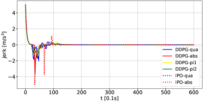
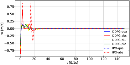
First, the results of the ACC model are depicted in Fig. 3 and Fig. 4, where the IPO method illustrates the optimal curve, while reinforcement learning often falls short of achieving such performance. The primary focus is on the final spacing error and acceleration change rate during the tracking process. Utilizing the squared reward function leads to a larger steady-state spacing error, as shown in Fig. 3, and the absolute value reward function induces significant peaks in the acceleration change rate throughout the control process, as shown in Fig. 4. However, employing PI-based methods one and two can reduce the final steady-state spacing error and result in smaller fluctuations in the acceleration change rate.
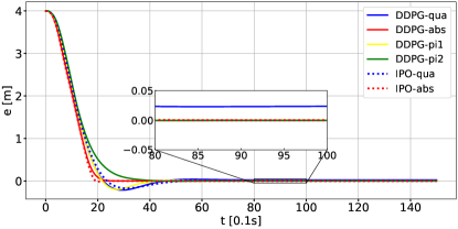
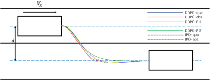
For the lane change model results, as illustrated in Fig. 5 and Fig. 6, the focus is on the final distance from the vehicle to the centerline of the second lane and the fluctuation in the wheel angle throughout the entire control process. Comparing the squared reward function with the absolute value reward function, as shown in Fig. 5, there is a difference of five orders of magnitude in the final distance steady-state error, as indicated in Table III. Additionally, the absolute value reward function exhibits larger fluctuations in the wheel angle change rate, as depicted in Fig. 6. The use of PI-based methods 1 and 2 demonstrates superior control performance. Fig. 7 depicts the lane change curves for the six different methods, with specific steady-state error values reflected in Table III.
| Method | ACC | Lane change |
|---|---|---|
| IPO-qua | 4.5e-7m | 2.4e-6m |
| DDPG-qua | 2.7e-1m | 2.3e-2m |
| DDPG-pi1 | 7.3e-3m | 1.8e-4m |
| DDPG-pi2 | 9.2e-3m | 4.9e-4m |
| IPO-abs | 1.1e-9m | 4.9e-7m |
| DDPG-abs | 2.9e-3m | 5.5e-5m |
V conclusion
This study utilizes PI-based reward functions to improve the control performance of reinforcement learning. The results indicate that using a squared reward function may lead to significant steady-state errors in certain system states, whereas an absolute value reward function may result in an unstable control process with spikes. Adopting PI-based reward functions not only reduces the steady-state error desired but also smoothens the entire control process.
References
- [1] K. Arulkumaran, M. P. Deisenroth, M. Brundage, and A. A. Bharath, “A brief survey of deep reinforcement learning,” arXiv preprint arXiv:1708.05866, 2017.
- [2] V. Mnih, K. Kavukcuoglu, D. Silver, A. A. Rusu, J. Veness, M. G. Bellemare, A. Graves, M. Riedmiller, A. K. Fidjeland, G. Ostrovski et al., “Human-level control through deep reinforcement learning,” nature, vol. 518, no. 7540, pp. 529–533, 2015.
- [3] Y. Li, “Deep reinforcement learning: An overview,” arXiv preprint arXiv:1701.07274, 2017.
- [4] F. L. Lewis, D. Vrabie, and V. L. Syrmos, Optimal control. John Wiley & Sons, 2012.
- [5] B. Kiumarsi, K. G. Vamvoudakis, H. Modares, and F. L. Lewis, “Optimal and autonomous control using reinforcement learning: A survey,” IEEE transactions on neural networks and learning systems, vol. 29, no. 6, pp. 2042–2062, 2017.
- [6] N. Hovakimyan and C. Cao, adaptive control theory: Guaranteed robustness with fast adaptation. SIAM, 2010.
- [7] R. S. Sutton and A. G. Barto, “Reinforcement learning: An introduction,” Robotica, vol. 17, no. 2, pp. 229–235, 1999.
- [8] L. Matignon, G. J. Laurent, and N. Le Fort-Piat, “Reward function and initial values: Better choices for accelerated goal-directed reinforcement learning,” in International Conference on Artificial Neural Networks. Springer, 2006, pp. 840–849.
- [9] S. Booth, W. B. Knox, J. Shah, S. Niekum, P. Stone, and A. Allievi, “The perils of trial-and-error reward design: misdesign through overfitting and invalid task specifications,” in Proceedings of the AAAI Conference on Artificial Intelligence, vol. 37, no. 5, 2023, pp. 5920–5929.
- [10] J. Eschmann, “Reward function design in reinforcement learning,” Reinforcement Learning Algorithms: Analysis and Applications, pp. 25–33, 2021.
- [11] Y. Luo, Y. Wang, K. Dong, Y. Liu, Z. Sun, Q. Zhang, and B. Song, “D2sr: Transferring dense reward function to sparse by network resetting,” in 2023 IEEE International Conference on Real-time Computing and Robotics (RCAR). IEEE, 2023, pp. 906–911.
- [12] J.-M. Engel and R. Babuška, “On-line reinforcement learning for nonlinear motion control: Quadratic and non-quadratic reward functions,” IFAC Proceedings Volumes, vol. 47, no. 3, pp. 7043–7048, 2014.
- [13] V. François-Lavet, P. Henderson, R. Islam, M. G. Bellemare, J. Pineau et al., “An introduction to deep reinforcement learning,” Foundations and Trends® in Machine Learning, vol. 11, no. 3-4, pp. 219–354, 2018.
- [14] T. Lilicrap, J. Hunt, A. Pritzel, N. Hess, T. Erez, D. Silver, Y. Tassa, and D. Wiestra, “Continuous control with deep reinforcement learning,” in International Conference on Learning Representation (ICLR), 2016.
- [15] Y. Lin, J. McPhee, and N. L. Azad, “Comparison of deep reinforcement learning and model predictive control for adaptive cruise control,” IEEE Transactions on Intelligent Vehicles, vol. 6, no. 2, pp. 221–231, 2020.
- [16] Q. Ge, Q. Sun, S. E. Li, S. Zheng, W. Wu, and X. Chen, “Numerically stable dynamic bicycle model for discrete-time control,” in 2021 IEEE Intelligent Vehicles Symposium Workshops (IV Workshops). IEEE, 2021, pp. 128–134.