Selective decision making and collective behavior of fish by the motion of visual attention
Abstract
Collective motion provides a spectacular example of self-organization in Nature. Visual information plays a crucial role among various types of information in determining interactions. Recently, experiments have revealed that organisms such as fish and insects selectively utilize a portion, rather than the entirety, of visual information. Here, focusing on fish, we propose an agent-based model where the direction of attention is guided by visual stimuli received from the images of nearby fish. Our model reproduces a branching phenomenon where a fish selectively follows a specific individual as the distance between two or three nearby fish increases. Furthermore, our model replicates various patterns of collective motion in a group of agents, such as vortex, polarized school, swarm, and turning. We also discuss the topological nature of visual interaction, as well as the positional distribution of nearby fish and the map of pairwise and three-body interactions induced by them. Through a comprehensive comparison with existing experimental results, we clarify the roles of visual interactions and issues to be resolved by other forms of interactions.
I Introduction
Collective motion and cluster formation are ubiquitously found in various organisms Vicsek2012 . Fish are no exception: there are swarm in which the direction of motion of fish is random, polarized school which shows directional movement, and vortex in which fish rotates around an axis Parrish2002 ; Lopez2012 ; Tunstrom2013 ; Terayama2015 . Schooling is induced not only by hydrodynamic interactions Partridge1980 ; Filella2018 ; Li2020 ; Ito2023 , but also for efficiently foraging food Harpaz2020 and avoiding predator Parrish2002 ; Radakov1973 , in which visual cues play an important role in transferring information among individuals Harpaz2020 ; Peshkin2013 ; Rosenthal2015 ; Poel2022 ; Hein2022 .
How does a fish process visual information in a school? Reacting to all neighboring fish within the field of view imposes a heavy load on the information processing system Dukas1998 , and it is considered to be less suitable for fish with relatively small brains Herbert2011 ; Hein2022 . In fact, zebrafish (Danio rerio) show selective decision making Burgess2010 ; Sridhar2021 : when there are two or three targets (i.e. light spots or virtual fish) within a certain distance in the range of eye sight, a zebrafish is attracted to one of the targets. In other words, a zebrafish selects and pays attention to one target, by truncating the visual information from other targets. A similar behavior is observed for fly and locust Sridhar2021 , indicating the commonness of selective decision making through visual information.
Fish schools have been modeled by agent-based models for decades Breder1954 ; Aoki1982 ; Huth1992 ; Huth1994 ; Niwa1994 with simple geometric criteria to determine the interaction: metric range Couzin2002 ; Kunz2003 ; Hemelrijk2008 , topological distance Inada2002 ; Viscido2005 ; Ito2022a ; Ito2022b , and Voronoi tessellation Gautrais2012 ; Calovi2014 ; Calovi2015 ; Filella2018 ; Deng2021 ; Liu2023 . Recent studies incorporate visual information for modeling the collective motion of fish Kunz2012 , bird Pearce2014 , and generic agents Lemasson2009 ; Lemasson2013 ; Bastien2020 ; Qi2023 ; Castro2023 . These models assume that an agent can integrate the information (e.g. distance and velocity) of all neighbors detected to decide its action. Some models Collignon2016 ; Sridhar2021 ; Gorbonos2023 ; Oscar2023 treat selective decision making under specific conditions. Collignon et al. Collignon2016 used a model stochastic model to reproduce the motion of 10 fish exhibiting burst-coast swimming in a tank with feeders. Sridhar et al. Sridhar2021 and the successive studies Gorbonos2023 ; Oscar2023 introduced a network model inspired by the Ising spin model and its phase transition. This model was applied to an agent interacting with a few virtual agents, and explained a bifurcation behavior of the agent’s position with the change of the distance between the targets.
In this paper, a comprehensive model of selective decision making and resultant collective motion based on visual stimuli. We introduce the notion of direction of attention induced by the stimulus and model its movement induced by the visual stimuli from neighbor fish. The fish interact via a repulsive, attractive and alignment interactions with the neighbors in the direction of attention. For a few fish, our model reproduces the bifurcation behavior observed in the previous experiment Sridhar2021 . For many fish, our model exhibits various patterns of emergent collective motion (vortex, polarized school, swarm and turning). Furthermore, we analyze the topological distance Herbert2011 and the pairwise and three-body forces Katz2011 from the viewpoint of visual interaction. The roles of visual information in the movement of fish is discussed by comprehensive comparison with the experimental results.
II Model
Our model is based on the eye system and experimentally observed behaviors of fish. First, neighbor fish are detected as projected images on the retina, and the signal is transmitted to the visual centers of the brain through retinal ganglion cells Pita2015 . The resolution of the images are determined by the number of ganglion cells. Their density is on the order of 104 cells/mm2 for zebrafish and golden shiner (Notemigonus crysoleucas), which use visual information as primary source of information. In addition, the resolution is higher in the forward direction than the backward: the density of the ganglion cells is higher in the rear side of the retina than in the front Pita2015 .
Second, an experiment on larval zebrafish shows that the visual interaction mainly depends on the vertical size of the image, and starts to depend weakly on the horizontal size as they grow Harpaz2021b . It is considered that fish adopts the vertical size as visual information to precisely measure the distance to neighbors, because the horizontal size easily changes by the relative heading angle of the neighbor as the fish has a slender body Harpaz2021b .
Third, the eyeball of fish moves well Kabayama1979 , and fish can track moving targets Kawamura1978 . The motion velocity of an image as well as its size is encoded on the brain Hein2022 . An experiment using golden shiner shows that a fish tends to follow the neighbors at a close distance in the front, as well as those moving at high relative speed. Sridhar2023 . Therefore, we incorporate the relative position and speed of the neighbor agents as the key elements for visual interaction.
Finally, the interaction forces are classified into repulsion, attraction, and alignment. Repulsion at short distances and attraction at large distances are demonstrated by a force map for golden shiner Katz2011 and mosquitofish (Gambusia holbrooki) Herbert2011 . The aligning interaction is found later for rummy-nose tetra (Hemigrammus rhodostomus) Calovi2018 . It is also worth mentioning that the orientational order of zebrafish is not explained by repulsion and attraction only Harpaz2021b . Integrating these properties, we construct our model as follows.
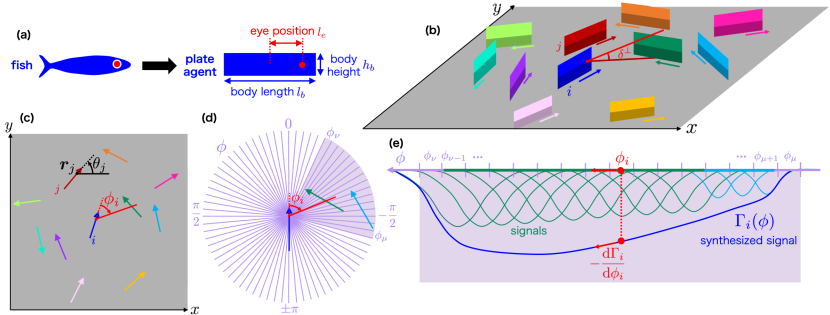
We model each self-propelled agent (fish) as a rectangular plate of length , height which has a monoeye at distance its center (Fig. 1(a)), and consider agents moving on a plane with no boundary (Fig. 1(b)). For the agent indexed by , we define the position of the eye and the velocity , where is the speed, and as the unit vector in the direction of motion ( is the angle of orientation).
The essential new feature of our model is the direction of visual attention specified by its angle (see Fig. 1(c)). We model the motion of as follows. As shown in Fig. 1(d), we divide the visual field into bins, and the number of bins is determined by the density of the ganglion cells. The angle of the -th bin () is denoted by . The vertical angular diameter (see Fig. 1(b)) and the relative speed of the neighbor in each bin is encoded as the visual information.
The image in each bin is transmitted as a signal that has a distribution in the “perception field” , which is described by a smooth signal function :
| (1) |
The angle dependence is given by the periodic function of ,
| (2) |
where gives the sharpness of a signal. Note that at , where the image is located. The function represents the density of ganglion cells and has the aforementioned front-back asymmetry parametrized by . The dependences on the vertical angular diameter and the relative speed of the image are described by and , respectively. (See Materials and Methods for details.)
The signals are superposed as a synthesized signal (see Fig. 1(e)):
| (3) |
and the angle of direction of attention is driven by the equation of motion
| (4) |
where is the characteristic time scale for . In other words, tends to approach a the local minimum of which is regarded as a potential function in the perception field, and the local minimum is deeper when the neighbor is closer, and further forward, and/or has higher relative speed.
Next, we introduce the equation of motion of the position of the -th agent. We adopt the variables () for the equation of motion Bastien2020 ; Qi2023 because, in addition to the change of the orientation, the change of the speed is also important for fish Katz2011 ; Herbert2011 . The equation for is
| (5) |
and the equation for is
| (6) |
where the mass is normalized as one, is the steady swimming speed, and is a constant. The self-propelled term corresponds to the balance between Newton’s drag force and the thrust force Gazzola2014 . The speeding force term includes the repulsion and attraction, and the angular velocity term includes the alignment in addition. is the relative heading angle between the focal agent and the neighbor detected at . is the average over the resolution angle region. Moreover, and correspond to the white Gaussian noises where and are the standard Wiener processes. In our model, we rescaled the parameter values for non-dimensionalization by a body length (BL) , timescale 1 sec, and body mass. (For example, the case in which the speed takes 1 means that the speed is 1 BL/sec.) The main control parameters of our model are the heterogeneity of the density of ganglion cells and the strength of alignment . (See Materials and Methods and SI Text for details of the formulation and definitions of the quantities measured in the simulation.)
III Results
III.1 Behavior of selective decision making
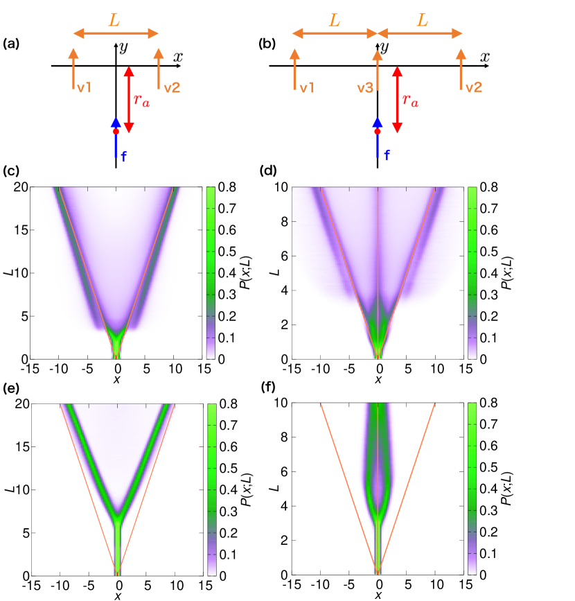
First, we demonstrate that our model exhibits selective decision making by reproducing some key features of the experimental results in Sridhar2021 . Following the study, we consider a focal agent following a few “virtual agents” that perform prescribed motion without interacting with the other agents. In the initial state (), as shown in Fig. 2(a)-(b), the focal agent f located at , is moving in the -direction with the speed and the angle of visual attention . The virtual agents vn (n are located at with the lateral distance and move along the -axis with the speed . The focal agent f obeys the time-evolution equations (4)-(6) and follows the virtual agents, which maintain their relative distance and velocity in the -direction. Here we set the parameters as and .
The focal agent fluctuates between different agents exhibiting a back-and-forth motion (Figs. S3(a),(d)), which has a characteristic timescale on the order of 10 time unit. Trajectories plotted in the moving frame of the virtual agents show that the focal agent follows the virtual agents from the back (Figs. S3(b),(e)).
To study the -dependence, we use the positional distribution of the focal agent in the moving frame and the marginal probability distribution which is obtained by integrating over the -axis. The plots of in Figs. S4, S5 show that the focal agent tends to be located behind the center of the virtual agents for a small , while the peak is split and located just behind each virtual agent for larger values of . This bifurcation behavior is more clearly seen in the plots of in Fig. 2(c),(d), which resemble the experimental results for fish Sridhar2021 . For two virtual agents (Fig. 2(c)), the focal agent is located at the center of the virtual agents for , and at the position of the virtual agents for . For three virtual agents (Fig. 2(d)), shows a three-way fork through two consecutive bifurcations; for , the focal agent is at the center of the three virtual agents; for , it resides at the center of v1 and v3 or the center of v2 and v3; for , it comes to the position of the virtual agents. At a very large distance (), the probability to follow the center virtual agent v3 becomes smaller than those for v1 and v2. See SI Text and Figs. S6,S7 for dependence on the other parameters.
We also tested an asymmetrical configuration of three virtual agents, where v3 is shifted to the right by the distance from the center (see Fig. S8(a)). For intermediate values of , the marginal probability distribution exhibits three peaks at the start of the three-way fork bifurcation (), instead of the four peaks for . The peaks are located at the right of v1, the left of v3, and between v2 and v3 (see Fig. S8(g)).
The behaviors are compared with those of a conventional particle model, which determines the motion of the focal agent by averaging the forces exerted by all virtual agents. For two virtual agents, we observed a bifurcation as shown in Fig. 2(e), but the distribution is determined by the equilibrium position of the averaged forces. In fact, the focal agent in the conventional particle model stays around a certain position between virtual agents instead of showing a back-and-forth motion (see Fig. S3(c),(f)). For three virtual agents, shows a two-way fork pattern that closes at large as shown in Fig. 2(f), instead of a three-way fork. The focal agent does not select and approach the left and right virtual agents.
III.2 Collective motion
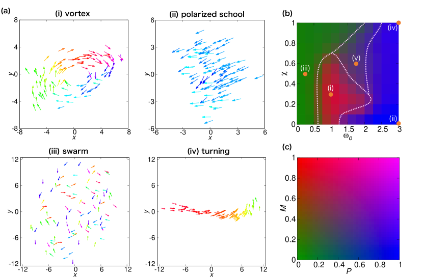
Next we study collective motion of many agents. For the initial condition, we randomly positioned 100 agents in a circle with a radius of 7 length unit. They have the same initial speed with the moving directions and angle of visual attention uniformly distributed in .
Varying the parameters , we obtained the collective patterns shown in Figs. 3(a),S9. They are classified into (i) vortex: agents rotating around a common axis, (ii) polarized school: agents aligned and moving coherently in the same direction, (iii) swarm: randomly oriented agents, (iv) turning: an elongated and curved cluster that intermittently develops from a polarized school (see also Fig. S9(a)), and (v) unsteady aggregation: a vortex collapses and then is transformed into a polarized school, which becomes a vortex again. This cycle occurs repeatedly with irregular time intervals (see Fig. S9(b)). See Supplemental Movies. S1-S5 for the dynamics of (i)-(v), respectively. The size of these patterns read from Fig. 3 is on the order of 10 length unit. The parameters that were used to study selective decision making in the previous section corresponds to the vortex pattern.
As quantitative measures of the patterns, we introduce the polar order parameter and the rotational order parameter (see Materials and Methods). For the steady patterns (i)-(iii), the order parameters rapidly converge to constants (see Fig. S10). For (iv), both and exhibit spikes that correspond to the emergence of curved clusters from a polarized school. For (v), both and oscillate with large amplitudes. For each parameter set (), we performed 25 simulations in the time domain to obtain the average values of and . The plot of and in the ranges , is shown in Fig. 3(b). We consider the noiseless case () to maximize the stability of the clusters. The plot gives a phase diagram of the collective patterns. As the strength of alignment increases, the agents get aligned and the cluster changes from a swarm to a vortex, and then to a polarized school or turning. For , the vortex emerges for -2.0, and the polarized school for -2.0. For , we obtain unsteady aggregation for , and turning for . Note that the emergence of swarm is controlled by and is almost independent of . See also Fig. S11 for a phase diagram based on other quantities.
The dependence on the number of agents is studied by keeping the same number density in the initial condition. As shown in Fig. S15(a),(b), the cluster tends to be stable for , but splits frequently for both and . (See SI Text and Figs. S12,S14 for a detailed analysis of the splitting and its dependence on the other parameters.)
III.3 Visual information and topological distance
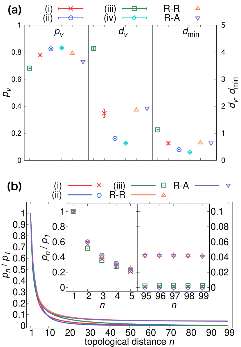
Here, we analyze the visual information of an agent in a cluster with 100 agents. We measure the occupancy ratio as the angular fraction of the images in the field of view, the average distance from the eye to the agents estimated by the vertical angular diameter, and the minimum distance to the neighbors . As shown in Fig. 4(a), is smaller and and are larger in the order of (iii) swarm, (i) vortex, (ii) polarized school, and (iv) turning. In particular, is close to the equilibrium distances of the forces and for (i) and (ii),(iv), respectively.
To study the visual screening effect by the neighbors, we define the relative occupancy ratio of the -th nearest neighbor (NN) as the fraction of the number of bins occupied by the image of NN in the bins occupied by all neighbors. We call the topological distance. As shown in Fig. 4(b), decays to almost zero at for the patterns (i),(ii), and (iii), which means that an agent cannot see all the neighbors in the cluster at a time. For comparison, we also study the case where 100 virtual agents are randomly positioned in a circle with a radius which is 7 length unit. Their orientation is either random (referred to as the random-random case) or aligned (the random-aligned case). Interestingly, for both cases, reaches to a non-vanishing constant at (see Fig. 4(b)), even though is larger and are smaller than that of a swarm (see Fig. 4(a)). It indicates that the visual field of an agent is screened more strongly by the clustering of real agents.
Next we verify the role of the visual attention in the screening effect. The probability for the angle of visual attention to lie within the bins occupied by NN also reaches zero as is increased (see Fig. S16(d)). Furthermore, the speeding force as a function of the topological distance (Fig. S17) is a strong attraction for large . However, because the probability for the visual attention is small for large , the expected value of the force is dominated by the repulsive force from near neighbors, which occupy most of the visual field.
III.4 Force map for pairwise and three-body interaction
Finally, in the presence of one or two neighbor agents, we consider their positional distribution (number density) and forces exerted by them. They are mapped as functions of the front-back position and the left-right position of the neighbors. Following the experiment Katz2011 , we measure the force by the acceleration of the focal agent and divide it into the speeding force and turning force, which are the components parallel and perpendicular to the direction of motion, respectively (see Fig. 5(a)).
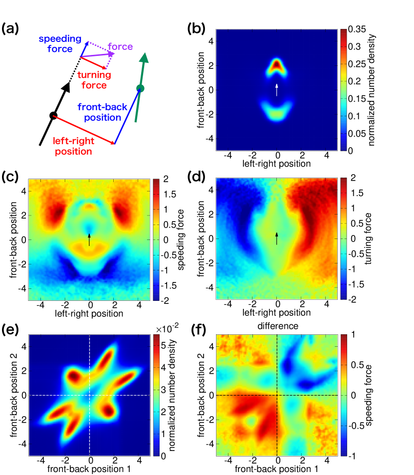
For two agents, the positional distribution of the neighbor has two peaks in the front and rear. The front peak is higher than the rear one, as shown in Fig. 5(b). Regarding the force map, the speeding force shows strong attraction at the left- and right-front and at the center-rear (see Fig. 5(c)). This forward-backward asymmetry is originated from the self-propelled force. As shown in Fig. S18(a), if we subtract the self-propelled force, the force map becomes forward-backward symmetric by construction of the speeding force of our model (see Eq. (11)). The turning force is strong at the left- and right-front (see Fig. 5(d)). This is interpreted by the alignment term, which is strong at the frontal side (see Eq. (V.2)). Moreover, as shown in Fig. S18(b),(d), the attractive speeding force and the attractive turning force increase with the relative speed of the neighbor, although we did not explicitly introduce such a dependence in the model equations (5),(6). (See SI Text and Figs. S18(c),(e) for the relative heading dependence of a neighbor.)
Next, we focus on three-body interaction. In particular, we analyze the relation between the front-back positions of the two neighbors and three-body interaction. As shown in Fig. 5(e), the normalized number density exhibits a characteristic aster pattern: this pattern indicates that the three agents tend to make a line-formation with a certain front-back distance between each pair. The speeding force of three-body interaction nearly vanishes at the equilibrium position which corresponds to the peak of the normalized number density (see Fig. S19(d)). To clarify the nature of three-body interaction, we subtract the averaged pairwise speeding forces from the total force. The pairwise forces are calculated assuming that only one neighbor exists at a time (see Fig. S19(e)). As shown in Fig. 5(f), the difference force reinforces the repulsion when both neighbors are at the front or rear of an agent, and also generates a restitution force when the two neighbors are in the front and rear. Furthermore, the turning component of the difference force is relatively small compared to the speeding component (see Fig. S19(i)).
IV Discussion
Our agent-based model incorporates selective decision making and collective motion. The visual signal is inspired by the behaviors of ganglion cells and eye system. In particular, we introduced the motion of the direction of visual attention. The interaction forces are modeled according to the experimental knowledge, and are averaged over the resolution region of the visual attention, instead of the conventional integrated pairwise interaction over all neighbors.
To confirm that our model actually shows the selective decision making, we used the virtual agents method. A focal agent selects a virtual agent spontaneously with the dynamical back-and-forth motion (see Figs. S3(a),(d)), and the marginal distributions exhibit the bifurcation behavior (see Fig. 2(c)-(d)) similar to those observed in fish and insects Sridhar2021 . In the case of zebrafish, the two- and three-way bifurcation for two and three virtual fish, respectively, occurs at BL Sridhar2021 . On the other hand, the bifurcation occurs at BL in our model. The difference might be explained by the resolution of the eyes; fish with a bigger body (e.g. golden shiner) has better resolution than zebrafish Pita2015 , for which our model might show a better agreement. In the presence of three virtual agents, the probability near the center one becomes small for large , in agreement with the zebrafish experiment Oscar2023 . For an asymmetrical configuration of virtual agents, the probability distribution shows three peaks (see Fig. S8(g)), which also catches the tendency for zebrafish Sridhar2021 . Furthermore, we have shown clearly that the conventional model which simply averages pairwise interactions from neighbor fish cannot reproduce the bifurcation process (see Fig. 2(e)-(f)).
Our model shows various patterns of collective motion (vortex, polarized school, swarm, and turning) as shown in Fig. 3(a). The size of the vortex and polarized school with 100 agents is about BL, in agreement with the size of collective patterns of 70 and 150 golden shiners (read from the Figures and Movies in Ref. Tunstrom2013 ). In the turning pattern, the cluster rapidly turns (see Fig. S9(a)), and it is different from the turning phase found in the previous model Filella2018 that maintains the curved shape. The parameter that characterizes the anisotropy of the ganglion cell density is estimated as about from an experiment (see Table LABEL:experimentalvalue and SI Text), and the vortex, polarized school, and swarm emerge in this region (see Fig. 3(b)). Regarding the dependence on the number of agents , the cluster is stable for , while a larger cluster tends to split into small clusters (see Fig. S15). The instability might be caused by confinement in 2D Calovi2014 ; Filella2018 ; in fact, a 3D model can reproduce a stable vortex for up to 10000 agents Ito2022a ; Ito2022b . For , we obtained frequent splitting, but it might be suppressed by the noise-governed interaction method as hypothesized for cichlid (Etroplus suratensis) Jhawar2020 .
The ratio of the visual field which is not filled by the other agents is (see Fig. 4(a)), which is consistent with the ratio -0.4 for 70-151 golden shiners Davidson2021 . In a cluster, the visual field of an agent is screened more by the neighbors comparing with the random configuration (see Fig. 4(b)). Regarding the topological distance, the first nearest neighbor contributes most to the repulsive speeding force and screening of the attraction (see Fig. S17(c)). On the other hand, for the angular velocity is not determined solely by the nearest neighbor, but several neighbors contribute nearly equally. (see Fig. S17(d)). In fact, the first nearest neighbor dominates the interaction in the case of mosquitofish Herbert2011 , and this dominance might be also responsible for the strong repulsive speeding force compared with the attractive speeding force and the turning force in a school of golden shiner Katz2011 .
Next we compare the positional distribution of neighbor fish and the force map, with the experimental results on golden shiner Katz2011 . For the positional distribution, our results reproduce the two peaks in the front and rear including their distances BL. We also reproduced the aster pattern in the correlation map of the front-back position of two neighbors (see Fig. 5(e)). In our model, the neighbor density is high in the front for both two and three agents (see Figs. 5(b),S19(a)), but golden shiner shows a forward-backward symmetrical distribution. Also, the correlation map of the left-right positions of two neighbors shows a peak at the center in our model (Fig. S19(f)), but the peak is split in the experiment.
We plotted the force map by the same method used in the experiment. For the speeding force, our model reproduces the small peaks in the front and rear due to the repulsion and broad peaks in the far region due to the attractive force. However, the experimental force map has a front-back symmetry of the speeding force, while our model shows asymmetrical patterns. The symmetry might be reproduced by incorporating anisotropic interaction in the present model. For dependence on the relative speed of a neighbor, the attraction increases with the relative speed (see Fig. S18(b),(d)), which is consistent with the experimental results. For three-body interaction, we reproduced the restitution speeding force (see Fig. 5(f)) and the fact that the turning force is given by the averaged pairwise force (see Fig. S19(i)). However, the reinforcement of the repulsive speeding force by the front or rear neighbors (see Fig. 5(f)) is small or vanishing in the experiment.
In summary, our visual model comprehensively reproduces the cooperative behaviors of fish, and give insight on decision making, collective motion, topological nature of interaction, and positional and force distributions. Our results are mostly consistent with the experiments, but additional elements in the interaction would be necessary to resolve the remaining issues. Inclusion of (i) complex neural system for integrating information from the left and right eyes Harpaz2021b , (ii) more precise dependences on the angular position and relative heading of a neighbor Calovi2018 , (iii) hydrodynamic signals via the lateral line Partridge1980 , and (iv) direct hydrodynamic interaction by the reverse Kármán vortex Li2020 ; Ito2023 will be interesting future directions.
V Materials and Methods
Here, we show the details of our model and the quantities measured in the simulation. See SI Text for more details of the definition of formulas, parameters, and the other information.
V.1 the visual signal
The ganglion cell density is represented by , which is a periodic function of :
| (7) |
where is the anisotropy parameter. The ratio between the cell densities at the front and rear side of the retina is given by .
Dependence on the vertical angular diameter is given by the function
| (8) |
where
| (9) |
is the relative distance of a neighbor, and is the limiting distance at which a body length can be identified.
Dependence on the relative speed of a neighbor is described by
| (10) |
is an increasing function of controlled by . Here, corresponds to the distance at which the pattern on the body of neighbor can be detected and the speed can be measured.
V.2 the equation of motion
The speeding force in Eq. (5) is given by
| (11) |
| (15) |
where is the equilibrium distance and is the distance that gives the maximum attractive force . When , gives the maximum repulsive force .
The angular velocity in Eq. (6) consists of the repulsion-attraction term and the alignment term Calovi2018 , as
| (16) |
The repulsion-attraction term is
| (21) |
where is the equilibrium left-right distance, which is smaller than due to the slender body of fish. We assume that fish can precisely detect the relative heading as well as the relative speed of a neighbor within . The alignment term is
where , is the characteristic length, and is the strength of alignment.
Finally, is the average of a quantity in the resolution angle region centered on : a set of bins includes the bin in , and is its size. The horizontal resolution angle is related to as .
V.3 the order parameters
The polar order parameter is defined as
| (23) |
It takes the maximal value 1 when the agents are completely aligned, and vanishes when the orientation of the agents is completely random. The rotational order parameter is defined as
| (24) |
where is the unit vector that gives the direction from the center of mass position . The rotational order parameter is large when the agents are rotating around a common axis in the same direction.
Supplementary Information
Supplementary Information is available from the below URL.
acknowledgement
We acknowledge financial support by JSPS KAKENHI Grant No. 23KJ0171 to S.I. and support by a research environment of Tohoku University, Division for Interdisciplinary Advanced Research and Education to S.I.
References
- (1) T. Vicsek and A. Zafeiris, Phys. Rep. 517, 71 (2012).
- (2) J. K. Parrish, S. V. Viscido, and D. Grünbaum, Biol. Bull. 202, 296 (2002).
- (3) U. Lopez, J. Gautrais, I. D. Couzin, and G. Theraulaz, Interface Focus 2, 693 (2012).
- (4) K. Tunstrøm, Y. Katz, C. C. Ioannou, C. Huepe, and M. J. Lutz, I. D. Couzin, PLoS Comput. Biol. 9, e1002915 (2013).
- (5) K. Terayama, H. Hioki, and M. Sakagami, Int. J. Semant. Comput. 9, 143 (2015).
- (6) B. L. Partridge and T. J. Pitcher, J. Comp. Physiol. 135, 315 (1980).
- (7) A. Filella, F. Nadal, C. Sire, E. Kanso, and C. Eloy, Phys. Rev. Lett. 120, 198101 (2018).
- (8) L. Li, M. Nagy, J. M. Graving, J. Bak-Coleman, G. Xie, and I. D. Couzin, Nat. Commun. 11, 5408 (2020).
- (9) S. Ito and N. Uchida, Phys. Fluids 35, 111902 (2023).
- (10) R. Harpaz, E. Schneidman, eLife, 9, e56196 (2020).
- (11) D. Radakov, Schooling in the Ecology of Fish (Wiley, New York, 1973).
- (12) A. Strandburg-Peshkin, C. R. Twomey, N. W. F. Bode, A. B. Kao, Y. Katz, C. C. Ioannou, S. B. Rosenthal, C. J. Torney, H. S. Wu, S. A. Levin, and I. D. Couzin, Curr. Biol. 23, R709 (2013).
- (13) S. B. Rosenthal, C. R. Twomey, A. T. Hartnett, H. S. Wu, and I. D. Couzin, Proc. Natl. Acad. Sci. U.S.A. 112, 4690 (2015).
- (14) W. Poel, B. C. Daniels, M. M. G. Sosna, C. R. Twomey, S. P. Leblanc, I. D. Couzin, P. Romanczuk, Sci. Adv. 8, eabm6385 (2022).
- (15) A. W. Hein, Curr. Opin. Neurobiol. 74, 102551 (2022).
- (16) R. Dukas, Constraints on information processing and their effects on behavior, in Cognitive Ecology: The Evolutionary Ecology of Information Processing and Decision Making (University of Chicago Press, Chicago, 1998)
- (17) J. E. Herbert-Read, A. Perna, R. P. Mann, T. M. Schaerf, D. J. T. Sumpter, and A. J. W. Ward, Proc. Natl. Acad. Sci. U.S.A. 108, 18726 (2011).
- (18) H. A. Burgess, H. Schoch, and M. Granato, Curr. Biol. 20, 381 (2010).
- (19) V. H. Sridhar, L. Li, D. Gorbonos, M. Nagy, B. R. Schell, T. Sorochkin, N. S. Gov, and I. D. Couzin, Proc. Natl. Acad. Sci. U.S.A. 118, e2102157118 (2021).
- (20) C. M. Breder, Ecology 35, 361 (1954).
- (21) I. Aoki, Bull. Jpn. Soc. Sci. Fish. 48, 1081 (1982).
- (22) A. Huth and C. Wissel, J. Theor. Biol. 156, 365 (1992).
- (23) A. Huth and C. Wissel, Ecol. Model. 75, 135 (1994).
- (24) H. Niwa, J. Theor. Biol. 171, 123 (1994).
- (25) I. D. Couzin, J. Krause, R. James, G. D. Ruxton, and N. R. Franks, J. Theor. Biol. 218, 1 (2002).
- (26) H. Kunz and C. K. Hemelrijk, Artif. Life 9, 237 (2003).
- (27) C. K. Hemelrijk and H. Hildenbrandt, Ethology 114, 245 (2008).
- (28) Y. Inada and K. Kawauchi, J. Theor. Biol. 214, 371 (2002).
- (29) S. V. Viscido, J. K. Parrish, and D. Grünbaum, Ecol. Model. 183, 347 (2005).
- (30) S. Ito and N. Uchida, J. Phys. Soc. Jpn. 91, 064806 (2022).
- (31) S. Ito and N. Uchida, Europhys. Lett. 138, 17001 (2022).
- (32) J. Gautrais, F. Ginelli, R. Fournier, S. Blanco, M. Soria, H. Chaté, and G. Theraulaz, PLOS Comput. Biol. 8, e1002678 (2012).
- (33) D. S. Calovi, U. Lopez, S. Ngo, C. Sire, H. Chaté, and G. Theraulaz, New J. Phys. 16, 015026 (2014).
- (34) D. S. Calovi, U. Lopez, P. Schuhmacher, H. Chaté, C. Sire, and G. Theraulaz, J. R. Soc. Interface 12, 20141362 (2015)
- (35) J. Deng and D. Liu, Bioinspir. Biomim. 16, 046013 (2021).
- (36) D. Liu, Y. Liang, J. Deng, and W. Zhang. Phys. Rev. E 107, 014606 (2023).
- (37) H. Kunz and C. K. Hemelrijk, Appl. Anim. Behav. Sci. 138, 142 (2012).
- (38) D. J. G. Pearce, A. M. Miller, G. Rowlands, and M. S. Turner, Proc. Natl. Acad. Sci. U.S.A. 111, 10423 (2014).
- (39) B. H. Lemasson, J. J. Anderson, and R. A. Goodwin, J. Theor. Biol. 261, 501 (2009).
- (40) B. H. Lemasson, J. J. Anderson, and R. A. Goodwin, Proc. R. Soc. B 280, 20122003 (2013).
- (41) R. Bastien and P. A. Romanczuk, Sci. Adv. 6, eaay0792 (2020).
- (42) J. Qi, L. Bai, Y. Wei, H. Zhang, and Y. Xiao, IEEE Internet Things J. 10, 10368 (2023).
- (43) D. Castro, F. Ruffier, and C. Eloy, arXiv:2305.06733 [physics.bio-ph] (2023).
- (44) B. Collignon, A. Séguret , and J. Halloy, R. Soc. open sci. 3, 150473 (2016).
- (45) D. Gorbonos, N. S. Gov, and I. D. Couzin, arXiv:2307.05837 [q-bio.NC] (2023).
- (46) L. Oscar, L. Li, D. Gorbonos, I. D. Couzin, and N. S. Gov, Phys. Biol. 20, 045002 (2023).
- (47) Y. Katz, K. Tunstrøm, C. C. Ioannou, C. Huepe, and I. D. Couzin, Proc. Natl. Acad. Sci. U.S.A. 108, 18720 (2011).
- (48) D. Pita, B. A. Moore, L. P. Tyrrell, and E. Fernández-Juricic, PeerJ 3, e1113 (2015).
- (49) R. Harpaz, M. N. Nguyen, A. Bahl, and F. Engert, Nat. Commun. 12, 6578 (2021).
- (50) A. Kabayama, G. Kawamura, and T. Yonemori, Bull. Jpn. Soc. Sci. Fish. 45, 1481 (1979).
- (51) G. Kawamura, A. Kabayama, and T. Yonemori, Bull. Jpn. Soc. Sci. Fish. 44, 567 (1978).
- (52) V. H. Sridhar, J. D. Davidson, C. R. Twomey, M. M. G. Sosna, M. Nagy, and I. D. Couzin, Phil. Trans. R. Soc. B 378, 20220062 (2023).
- (53) D. S. Calovi, A. Litchinko, V. Lecheval, U. Lopez, A. P. Escudero, H. Chaté, C. Sire, and G. Theraulaz, PLOS Comput. Biol. 14, e1005933 (2018).
- (54) M. Gazzola, M. Argentina, and L. Mahadevan, Nat. Phys. 10, 758 (2014).
- (55) J. Jhawar, R. G. Morris, U. R. Amith-Kumar, M. D. Raj, T. Rogers, H. Rajendran, and V. Guttal, Nat. Phys. 16, 488 (2020).
- (56) J. D. Davidson, M. M. G. Sosna, C. R. Twomey, V. H. Sridhar, S. P. Leblanc, and I. D. Couzin, J. R. Soc. Interface 18, 20210142 (2021).