Enhancing Hemodynamic Parameter Estimations: Nonlinear Blood Behavior in 4D Flow MRI

Abstract

Hemodynamic parameters have been estimated assuming a Newtonian constant viscosity, even when blood exhibits shear-thinning behavior. This article investigates the influence of blood rheology and hematocrit percentage on estimating Wall Shear Stress (WSS) and Energy Loss ($E_{L}$) at different time instants of the cardiac cycle, as well as the Oscillatory Shear Index (OSI). We specifically focus on a hematocrit-dependent power-law non-Newtonian model, considering a wide range of hematocrit values. The rheological parameters are obtained from experimentally fitted data reported previously. This study contributes to understanding the impact of blood rheology on hemodynamic parameter estimations using both in-silico and in-vivo aortic 4D Flow magnetic resonance images. Across all cases, we systematically compared WSS, $E_{L}$, and OSI parameters using Newtonian and power-law models, highlighting the crucial role of blood rheology in accurately assessing cardiovascular diseases.

1 Introduction

Hemodynamic parameters estimated from 4D flow Magnetic Resonance (MR) images such as Wall Shear Stresses (WSS), Oscillatory Shear Indexes (OSI), and Energy Loss (E${}_{\textit{L}}$) have been successfully used for the assessment of several cardiovascular diseases in large vessels, including Bicuspid Aortic Valve (BAV) [1], aortic coarctations [2], stenosis [3], among others [4]. These parameters need as input a blood viscosity $\mu$, which in most of the cases is assumed constant and within the range of $0.03$ to $0.045$ poise [5, 6, 7, 8, 9, 10]. This assumption has been accepted in the cardiovascular MRI community for the past decades, serving as the gold standard for the estimation of viscosity-dependent hemodynamic parameters from 4D flow MR images. However, the blood viscosity has an intrinsic shear-thinning nonlinear behavior (i.e., viscosity decreases as increasing shear rates) that, to the author’s knowledge, has not been systematically considered in estimating these parameters.

Blood is a non-homogeneous and non-linear fluid comprising red blood cells, white blood cells, and platelets suspended in plasma. The behavior of blood can be modeled using continuum mechanics and experimental data, leading to non-Newtonian constitutive models. Generally, blood exhibits shear-thinning behavior, primarily dependent on the hematocrit (Hct) percentage. This shear-thinning behavior can be effectively described using models such as the power-law [11, 12], Carreau-like [13, 14, 15], Cross [16, 12], and Casson models [17]. Considering that the power-law has been successfully fitted to a wide range of Hct percentages under physiological temperatures [18, 19, 20], we have adopted this model as a suitable candidate for explaining blood’s fluid behavior.

Increased Hct can result from dehydration and polycythemia, while decreased values can be caused by anemia, overhydration [21, 19, 18, 20], kidney failure, pregnancy, or chronic inflammatory conditions [22]. Although Hct can range from $10\%$ to $70\%$ in individuals with these conditions, the normal range is $47\pm 7\%$ for men and $42\pm 6\%$ for women [23]. Besides, shear rate depends on spatial and temporal blood flow characteristics, opening up the question of whether Newtonian modeling, accepted by the MRI community, truly represents a whole cardiac cycle. In this regard, including a non-Newtonian rheological behavior could generate potential differences in hemodynamic parameters across patients, especially in non-physiological blood conditions.

The influence of blood rheology has been studied in different contexts of hemodynamics. For example, a shear-thinning viscosity depending on the Hct was employed to estimate hemodynamic parameters from in-vivo data in the circle of Willis in children and adults with sickle cell disease [24] and for flow analysis of the left ventricle (LV) [25]. In [26], a numerical study of the influence of the hematocrit level in blood was developed considering anemic and physiological patients in a simplified carotid artery, finding that there are differences regarding the frequency of vortex shedding and flow bifurcation between the carotid outlet branches. In-silico studies involving the normal aorta [27], aortic aneurysm, and the venous system [28], as well as in-vitro phantom experiments with geometries resembling Fontan patients [29] and prosthetic heart valves [30], have also been conducted.

Despite the valuable insights provided by the aforementioned hemodynamics works where the shear-thinning rheological behavior has been incorporated in the blood flow modeling, it is essential to mention some limitations and open questions. The effect of rheological behavior in large vessels like the aorta has not been analyzed in detail [24, 25]. The impact of blood hematocrit has not been studied in wide ranges [29, 28, 27], or has not addressed their influence on specific hemodynamic parameters like WSS and OSI [30]. Additionally, none of these studies have thoroughly assessed the potential impact of imaging artifacts on their results, such as partial volume effects and signal decay, among other factors, especially in MRI.

In this work, we propose that the shear-thinning behavior of blood significantly impacts the quantification of hemodynamic parameters and should be considered. To verify this hypothesis, we addressed three main research questions. First, we examined the necessity of using nonlinear rheology models instead of the usual linear models. Second, we investigated whether differences in hemodynamic parameters induced by blood rheology are observable despite MRI artifacts. Third, we explored how the blood shear-thinning behavior at different Hct values impacts the estimation of hemodynamic parameters from 4D Flow MR images compared to the gold standard procedure and viscosities fitted by Hct values. These questions were addressed by evaluating in-silico and in-vivo (of patients with hypertrophic cardiomyopathy) aortic 4D Flow images to test our hypothesis. WSS, $E_{L}$, and OSI estimations were compared when considering the classic Newtonian and the power-law models fitted to a wide range of Hct percentages. This article contributes to further understanding the discussed aspects and lays the groundwork for more specific studies related to MRI and CFD.

2 Methods

2.1 Mathematical modeling

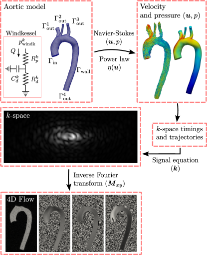
Figure 1: Simulation workflow for generating 4D Flow MR images. First, the aortic model serves as input to the MAD library, where the Navier-Stokes equations with nonlinear viscosity are solved. Subsequently, $k$-space locations and sequence timings are generated using parameters from Table 3, and the signal equation in 2.4 is evaluated. Trapezoidal MRI gradients are considered for the generation of sequence timings.

Let $\Omega\in\mathbb{R}^{3}$ be the three-dimensional computational domain, whose two-dimensional boundaries are decomposed in disjoint subsets such that $\partial\Omega=\Gamma_{\text{in}}\cup_{k=1}^{l}\Gamma_{\text{out}}^{k}\cup\Gamma_{\text{wall}}$, referring $\Gamma_{\text{out}}$ for the outlets, $\Gamma_{\text{in}}$ for the inlet, and $\Gamma_{\text{wall}}$ for the artery walls. The incompressible Navier-Stokes (NS) equations consist of finding the velocity vector field ($\boldsymbol{u}$) and the pressure ($p$), such that:

$$\rho\frac{\partial\boldsymbol{u}}{\partial t}+\rho\boldsymbol{u}\cdot\nabla\boldsymbol{u}+\nabla p-\nabla\cdot(2\mu\dot{\boldsymbol{\varepsilon}}) =0 \text{ in }\Omega,$$ (2.1a)

$$\nabla\cdot\boldsymbol{u} =0 \text{ in }\Omega,$$ (2.1b)

$$\boldsymbol{u} =\boldsymbol{g}(x,t) \text{ on }\Gamma_{\text{in}},$$ (2.1c)

$$\boldsymbol{u} =0 \text{ on }\Gamma_{\text{wall}},$$ (2.1d)

$$(2\mu\dot{\boldsymbol{\varepsilon}}-pI)\cdot\boldsymbol{n} =-p^{k}_{\text{wk}} \text{ on }\Gamma_{\text{out}}^{k},$$ (2.1e)

being $k=1,\ldots,l$ the outlet counter, and where $\dot{\boldsymbol{\varepsilon}}=\{\nabla\boldsymbol{u}+(\nabla\boldsymbol{u})^{T}\}/2$ denotes the symmetrical gradient operator, and $g(x,t)$ is an arbitrary spatially and temporarily dependent boundary condition. The blood properties are the fluid density $\rho$ and the dynamic viscosity $\mu$. In addition, to model the downstream fluid we couple the 3D-NS equations with the reduced 0D three-parameters Windkessel models [31] (see Figure 1), as it is typically done in the literature [32, 33, 34, 35]. This approach boils down to solving an ordinary differential equation (ODE) for each outlet domain, such that:

$$p^{k}_{\text{wk}}=R_{p}Q^{k}(\boldsymbol{u})+p^{k}_{d},\quad k=1,\ldots,l,$$ (2.2a)

$$C^{k}_{d}\frac{dp^{k}_{d}}{dt}+\frac{p^{k}_{d}}{R^{k}_{d}}=Q^{k}(\boldsymbol{u}),\quad k=1,\ldots,l.$$ (2.2b)

where $Q^{k}(\boldsymbol{u})=\int_{\Gamma_{\text{out}}^{k}}\boldsymbol{u}~{}ds$, and the parameters $R^{k}_{d}$, $C^{k}_{d}$, $R^{k}_{p}$, are the distal resistance, distal capacitance, and proximal resistance, respectively. The ODE should be closed with an adequate initial condition $p^{k}_{d,0}$. This configuration reproduces the downstream vascular tree and interacts with the 3D-NS model by setting an inwards force. It must be noted that we are using 0D parameters adjusted initially within a Newtonian context. It is a future endeavor of the researchers also to consider the blood rheology on the downstream fluid model.

In the non-Newtonian context, the viscosity $\mu$ is called apparent viscosity. The non-Newtonian blood-thinning behavior is incorporated in this work through the power-law model:

$$\mu_{\mathrm{PL}}=m\dot{\gamma}^{n-1},$$ (2.3)

where $\dot{\gamma}=\sqrt{2\dot{\boldsymbol{\varepsilon}}:\dot{\boldsymbol{\varepsilon}}}$ and the sub-index PL stands for power-law. The values used for $n$ and $m$, fitted according to the ones proposed in [19, 20, 18], came from experimental studies and were characterized at a physiological temperature of 37 ^∘C (see Table 1). The role of the power-law index parameter, $n$, is to define the rheological behavior of the fluid. When $n=1$ the Newtonian model is recovered. Shear-thinning fluids like blood are characterized by $n<1$. The parameter $m$ is the consistency index.

Table 1: Viscosities used for CFD simulations and estimation of hemodynamic parameters from 4D Flow images

Htc	Newtonian	Power law,	Newtonian fitted
	$\mu_{\mathrm{N}}$ ($10^{-3}$ Pa$\cdot$s)	$m$ ($10^{-2}$ Pa$\cdot$sn), $n$	$\mu_{\mathrm{NF}}$ ($10^{-3}$ Pa$\cdot$s)
10	3.0, 3.5, 4.0, 4.5	1.0800, 0.6800 [20]	2.1763
35		0.8882, 0.8254 [19]	3.6530
45		1.4821, 0.7755 [19]	4.7724
60		3.1800, 0.7060 [18]	7.4104
70		4.3450, 0.6760 [18]	8.7828
28	3.0, 3.5, 4.0, 4.5	0.6264, 0.8363 [18]	2.7220
40		1.1203, 0.8045 [19]	4.1482
50		1.9537, 0.7542 [19]	5.6303
$m$ and $n$ values were used to calculate $\mu_{\mathrm{PL}}$ by evaluating Equation 2.3.
Values used only for the quantification of in-vivo data.
Only third and fourth columns were used for CFD simulations.

2.2 Generation of 4D Flow MR images

Given the blood velocity $\boldsymbol{u}=(u_{x},u_{y},u_{z})$ obtained from CFD simulations, 4D Flow MR images were generated evaluating the signal equation given in (2.4), which depends on magnetization at the thermal equilibrium $M_{0}(\boldsymbol{r})$, velocity encoding sensitivity (VENC), blood velocity $u_{a}$ (with $a=x,y,z$), and relaxation time of the blood $T_{2}^{*}(\boldsymbol{r})$.

$$s^{a}(\boldsymbol{k}(t)) =\int_{B}M(\boldsymbol{\boldsymbol{r}},t)e^{-\boldsymbol{i}2\pi\boldsymbol{k}(t)\cdot\boldsymbol{r}(t)}~{}d\boldsymbol{r},$$ (2.4a)

$$M(\boldsymbol{\boldsymbol{r}},t) =M_{0}(\boldsymbol{r})e^{-\boldsymbol{i}\pi/\text{VENC}u_{a}(\boldsymbol{r})}e^{-t/T_{2}^{*}(\boldsymbol{r})},$$ (2.4b)

In the preceding expressions, $\boldsymbol{k}(t)$ denotes how Fourier space is measured during signal acquisition, and this measurement varies based on the chosen acquisition sequence. Constructing $\boldsymbol{k}(t)$ requires careful consideration of the hardware limitations of the scanner. For instance, velocity and phase-encoding gradients rely on the maximum slew rate and amplitude of the gradient system. Additionally, the readout gradient is affected by the sampling frequency of the ADC. These dependencies collectively influence the echo time, determining the time at which each $k$-space point is measured.

During signal measurement, the positions of spins change over time due to the blood dynamics. This effect is accounted for by employing a first-order approximation of the spins’ positions $\boldsymbol{r}(t)$ around $t_{k}$, typically expressed as:

$$\boldsymbol{r}(t)=\boldsymbol{r}(t_{k})+\boldsymbol{u}(t_{k})(t-t_{k})+\mathcal{O}(t^{2}),$$ (2.5)

where $t_{k}$ represents the time where the image was taken.

No field inhomogeneities were considered during the evaluation of (2.4), and the integral was calculated for each $k$-space location using the finite elements (FE) method.

All the steps described in this section were implemented in the PyMRStrain library, previously used to generate synthetic strain phantoms [36, 37, 38].

3 Experiments

3.1 Flow simulation

We set our computational domain to be a tetrahedral mesh of a patient-specific aorta model (see Figure 1), obtained from the Vascular Model Repository [2, 39, 40, 41]. The mesh comprises 127,131 vertices and 719,419 tetrahedrons.

The governing equations of the flow given in (2.1) were solved using the finite-elements method with piece-wise linear Lagrange elements for $\boldsymbol{u}$ and $p$. To overcome the well-known inf-sup constraints [42], a Brezzi-Pitkäranta stabilization term was added to the formulation [43], alongside a streamline upwind term to ensure stability for highly convective flows [44, 45]. Similar stabilization techniques in non-Newtonian fluids have been tested and analyzed in detail in [46, 47]. Additionally, the back-flow stabilization method proposed in [48, 49] was incorporated into all the simulations.

Table 2: Parameters for CFD simulations

FEM parameter	Value
Time step ($\Delta t$)	$9.37\times 10^{-4}$ sec
Nonlinear tolerance ($\delta_{p}$)	$10^{-4}$
Backflow parameter ($\beta$) [48, 49]	0.2
Windkessel Parameter	$\Gamma_{\text{out}}^{1}$, $\Gamma_{\text{out}}^{2}$, $\Gamma_{\text{out}}^{3}$, $\Gamma_{\text{out}}^{4}$
Proximal resistance ($R^{k}_{p}$)	274, 1300, 791, 141
Distal resistance ($R^{k}_{d}$)	5675, 19663, 10048, 2066
Distal capacitance ($C^{k}_{d}\times 10^{-4}$)	5.08, 1.4416, 2.788, 13.6904
Distal pressure ($p^{k}_{d,0}$)	107325, 107325, 107325, 107325

The inlet boundary condition, as defined in (2.1c), is represented by $g(x,t)=u_{\text{max}}(t)\mathcal{S}(x)$. Here, $u_{\text{max}}$ is obtained from phase-contrast MRI measurements [2]. The function $\mathcal{S}$ characterizes the spatial distribution of the Dirichlet condition, resembling a laminar parabolic fluid profile. Both $u_{\text{max}}$ and $\mathcal{S}$ are shown in Figure 2.

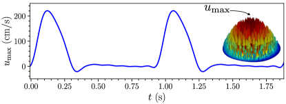
Figure 2: Inlet boundary condition $u_{\text{max}}(t)$ and parabolic flow profile used as Dirichlet boundary condition on $\Gamma_{\text{in}}$.

We employed a second-order finite difference formula for temporal discretization with a time step size of $\Delta t=9.37\times 10^{-4}$ s (equivalent to 1000 steps per cardiac cycle). The simulation covered two cardiac cycles, with only the last cycle considered in the analysis to avoid nonphysical solutions.

The non-linear terms in (2.1), i.e., the convection and the fluid constitutive, were linearized using a Picard fixed point approach, with an $H^{1}\times L^{2}$ error tolerance of $\delta_{p}=10^{-4}$. The coupling with the Windkessel model is done semi-implicitly, using a 4th-order Runge-Kutta scheme for the ODE.

We use the software MAD [50] to assemble the discrete equations and invert the linear systems. The software is built upon the linear algebra library PETSc [51], and the computations are done with up to 72 CPU cores in parallel. A summary of the numerical simulation parameters is given in Table 2.

These equations were solved for Newtonian (constant) viscosities ($\mu_{\mathrm{N}}$) usually found in the literature when estimating hemodynamic parameters, Newtonian (constant) viscosities fitted by Hct ($\mu_{\mathrm{NF}}$), and power-law viscosities (nonlinear) also adjusted by Hct ($\mu_{\mathrm{PL}}$). The process to obtain $\mu_{\mathrm{NF}}$ involved the following steps: (1) Defining values of $\dot{\gamma}$ within the range $[9,429]$ 1/s in increments of 4, chosen based on available measurements in the literature. (2) Evaluating the power-law described in (2.3) for the parameters in Table 1, resulting in a set of discrete points. (3) Finally, fitting the model $\mu_{\mathrm{NF}}=c$ (with $c\in\mathbb{R}$) to the data points using least squares. All these values can be found in Table 1.

3.2 Image generation

Table 3: Parameters for 4D flow image generation

Imaging parameter	Value
VENC (m/s)	$1.5$, $2.0$, $2.5$
Matrix size	$66\times 55\times 120$
Voxel size (mm$\times$mm$\times$mm)	$2\times 2\times 2$
Oversampling factor	$2$
Cardiac phases	$30$
Time spacing (ms)	$32.0$
$T_{2}^{*}$ (ms) [52]	$254.0$
ADC bandwidth (kHz) [53]	$128.0$
Slew-rate (mT/m/s) [54]	$195.0$
Max. gradient amplitude (mT/m) [54]	$30.0$
These parameters give echo-times of 1.85, 1.74, and 1.66 ms for VENCs of 1.5, 2, and 2.5 m/s, respectively.

4D Flow MR data was generated using imaging parameters (e.g, voxel size, number of cardiac phases, and VENC) from the 2023 4D Flow MRI consensus (see Table 3) [55]. Hardware parameters such as maximum gradient amplitude, slew-rate, and ADC frequency bandwidth, which dictated sequence timings and the image quality, were taken from [53] and [54]. For each Hct, three gradient-echo images were simulated, encompassing three distinct velocity encoding (VENC) values.

To emulate realistic conditions, Gaussian noise was introduced, with a standard deviation set at 2.5% of the maximum amplitude of the magnitude of the complex signal. The noise was added to both the real and imaginary channels, resulting in three distinct noise levels in the estimated velocity, each corresponding to the different VENCs. Two of three VENCs have aliasing artifacts, introducing discontinuities in the velocity field.

The MRI signals were generated from CFD simulations using the power-law model and constant viscosities adjusted by Hct. The reconstruction of 4D Flow images involved performing the inverse Fourier transform of the signal, as defined in equation (2.4).

3.3 Comparing hemodynamic parameters

WSS vector ($\boldsymbol{t}_{\mathrm{WSS}}$), OSI, $E_{L}$ were estimated as follows:

$$\boldsymbol{t}_{\text{WSS}} =\boldsymbol{l}\times\left\{\left(2\mu\dot{\boldsymbol{\varepsilon}}\boldsymbol{l}\right)\times\boldsymbol{l}\right\}$$ (3.1a)

OSI $$=\frac{1}{2}\left(1-\frac{\left\lVert\int_{0}^{T}2\mu\dot{\boldsymbol{\varepsilon}}\boldsymbol{l}~{}dt\right\rVert}{\int_{0}^{T}\lVert 2\mu\dot{\boldsymbol{\varepsilon}}\boldsymbol{l}\rVert~{}dt}\right)$$ (3.1b)

$$E_{L} =\mu\phi_{\boldsymbol{u}}V$$ (3.1c)

where $\boldsymbol{l}$ denotes a unitary inward unit surface normal vector, $2\mu\dot{\boldsymbol{\varepsilon}}\boldsymbol{l}$ the shear stress, $T$ the duration of the cardiac cycle, $V$ the Voronoi volume for each node in the FE mesh, and $\phi_{\boldsymbol{u}}$ the viscous dissipation described previously in [8]. When computing these parameters in the non-Newtonian case, the apparent viscosity varies spatially, which must be considered in the quantification.

These three biomarkers were chosen due to their direct dependence on viscosity. The boundary layer near the vessel wall, affected by blood rheology, can undergo thinning or thickening, impacting velocity gradients and, consequently, viscosity. Evaluating $\boldsymbol{t}_{\text{WSS}}$ becomes crucial in this context. OSI assesses temporal changes in shear stress induced by viscosity variations and flow dynamics, aspects not covered by $\boldsymbol{t}_{\text{WSS}}$. Lastly, $E_{L}$ measures how energy dissipates within the flow due to viscous fluid interactions, which is also susceptible to changes in viscosity.

The three quantities specified in (3.1) were estimated using the 4D Flow Matlab Toolbox [56]. This toolbox utilizes a previously validated FE scheme [57] to compute various hemodynamic and geometrical parameters from 4D Flow MRI data [1]. To address aliasing artifacts within the phase of the image, the single-step Laplacian method, outlined in [58], was employed, a technique also integrated into the toolbox.

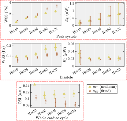
Figure 3: Mean values and standard deviations of WSS, OSI, and $E_{L}$ across four aortic segments estimated from simulated images obtained from CFD simulations with power-law and fitted-Newtonian viscosities. Estimations were performed using the same viscosity models employed in the simulations.

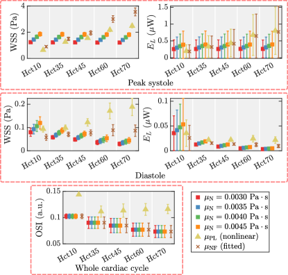
Figure 4: Mean values and standard deviation of WSS, OSI, and $E_{L}$ across four aortic segments estimated from simulated images obtained from CFD simulations with nonlinear rheology. Estimations were made using Newtonian, fitted-Newtonian, and power-law viscosities.

The comparison of hemodynamic parameters, estimated from synthetically generated 4D Flow images, was carried out considering three scenarios:

1. A fully non-linear viscosity scenario, meaning that both the CFD simulations used for image generation and the parameters were computed considering the shear-thinning effect.

2. A fully linear viscosity approach where both the CFD simulation used for image generation and the parameters were obtained using Newtonian fitted viscosities.

3. A mixed approach where the CFD simulations used for image generation considered shear-thinning phenomena and the parameters were computed with constant Newtonian viscosities ($\mu_{\mathrm{N}}$), Newtonian viscosities fitted by Hct levels ($\mu_{\mathrm{NF}}$), and power-law viscosities ($\mu_{\mathrm{PL}}$) fitted by Hct levels.

Scenarios 1 and 2 aimed to test our modeling choice and assess whether non-linear viscosity should be considered for the selected hemodynamic parameters. On a different note, the third scenario demonstrates a common practice in the community. In the context of the present study, $\mu$ values in (2.1) and (3.1) are replaced by $\mu_{\mathrm{N}}$, $\mu_{\mathrm{NF}}$, and $\mu_{\mathrm{PL}}$ to obtain results for the different scenarios. These viscosity values can be found in Table 1.

To perform comparisons, the aortic geometry was segmented into four sections, and mean values of all hemodynamic parameters were computed for each segment at peak systole and diastole (refer to Figure 5).

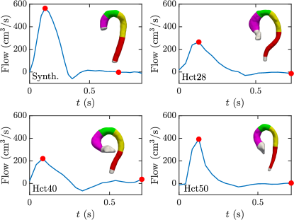
Figure 5: Flow curves obtained from 4D Flow images at the ascending aorta (at the level of the pulmonary bifurcation) and aortic segments considered in all the analyses. The top-left image shows the measurement made of the synthetic dataset, whereas the remaining figures show the curves obtained from the patient data.

3.4 In-vivo data

In-vivo gadolinium-enhanced triple-VENC 4D Flow images were acquired from three patients with hypertrophic cardiomyopathy, using a 3.0T Achieva scanner (Philips Healthcare, Best, The Netherlands). Imaging parameters considered an acquired voxel size of 1.7x1.7x2.0 mm, VENCs of 50, 150, and 450 cm/s, temporal resolution of 40 ms, and 15 to 21 frames depending on heart rate. Further details of the sequence and reconstruction can be found in [59]. Each patient had available Complete Blood Counts (CBCs). The experiments took place at Nippon Medical School Hospital, with the study approved by their IRB, and all subjects providing written informed consent. The patients had Hct levels of 28%, 40%, and 50%.

4 Results

This section focuses only on results derived from images with a VENC of 250 cm/s, the noisiest case for 4D Flow velocity. Other cases are provided in Suplementary Figure S1 since their outcomes are almost identical to those presented here. In the following results, the magnitude of $\boldsymbol{t}_{\text{WSS}}$ (namely WSS), OSI, and $E_{L}$ are reported. Additionally, only the mean values across the four segments of each hemodynamic parameter, along with their respective standard deviations, are showed in this section to avoid visual cluttering. Figures with regional information for each segment are presented in the Supplementary Figures S2 to S4.

Figure 3 shows the comparison between hemodynamic parameters calculated from 4D Flow MRI images generated from CFD simulations, as explained in sections 2.B and 2.C, obtained using Newtonian and power-law viscosities for the simulation and hemodynamic parameters estimation. The results show noticeable differences in WSS and OSI but small differences in $E_{L}$. The maximum differences across Hct levels, relative to the power-law model, were 41% and 36% for WSS and -5% and -34% for $E_{L}$ in systole and diastole respectively, while for OSI is -29%. These discrepancies demonstrate that the use of a Newtonian linear model of the blood could only be reliable as a surrogate model if the goal is to assess only the $E_{L}$ at any Hct level, whereas the calculations for WSS and OSI justify the inclusion of nonlinear rheology. In Supplementary Figures S5 and S6, the same comparison is done by computing the WSS directly from the CFD simulations (without generating a synthetic 4D Flow image), leading to the same conclusions.

Figure 4 shows the mean values of WSS, $E_{L}$, and OSI estimated from the synthetic 4D Flow images in the mixed scenario. It is noticeable that during peak systole and with an Hct of 45%, corresponding to a healthy Hct level, using the power-law estimations as reference, differences in WSS and $E_{L}$ estimated using Newtonian (5% and -10% for the best case, respectively) and fitted-Newtonian (26% and -5%, respectively) viscosities are visually small. However, as the Hct varies, the disparities in the estimated WSS become notable. Relative to the power-law approach, differences observed using fitted-Newtonian viscosities reach around 40% for extreme values of Hct, while Newtonian viscosities yield values ranging from 94% to -27%, considering the best cases. These differences are based on the most favorable case for extreme Hct levels of 10 and 70, respectively. This pattern is similar for $E_{L}$ and substantial standard deviations are also observed across aortic segments in this parameter. However, compared to power-law estimations, values obtained using fitted-Newtonian viscosities showed relative differences around 5% for any Hct level, while Newtonian viscosities yielded relative differences in the range of 30% and -51% in the most favorable cases.

Nonetheless, these behaviors differ during diastole. When compared to the power-law, estimations derived from Newtonian and fitted-Newtonian viscosities tend to exhibit lower relative differences in both WSS and $E_{L}$ for Hct values of 10 and 35. For instance, differences in WSS for an Hct of 10% are -0.4% for Newtonian and -38% for fitted-Newtonian viscosities, while for $E_{L}$, they are 0.3% and -27%, respectively. These differences become more pronounced as the Hct increases, reaching values of -77% in both WSS and $E_{L}$ using Newtonian viscosities, and -54% and -56% for WSS and $E_{L}$ using fitted-Newtonians, respectively.

The differences between peak systole and diastole are more noticeable when examining the OSI, which quantifies shear stress variations throughout the cardiac cycle. Figure 4 demonstrates larger OSI values in estimations using the power-law, suggesting more observable discrepancies in shear stress across the cardiac cycle when considering nonlinear blood rheology. Differences in Newtonian and fitted-Newtonian estimations are -29% in (Hct-averaged) in both cases relative to the power-law.

During systole, it is notable that both WSS and $E_{L}$ estimated using Newtonian viscosities remain nearly consistent across different Hct levels. However, during diastole, these estimations decrease as the Hct increases. The trend is also observed in OSI, which decreases for Newtonian viscosities as Hct levels increase. These behaviors can be attributed to the similar flow patterns (i.e., velocity gradients) found for any Hct at peak systole, while in diastole, the flows differ significantly (see Figure S6).

Figures 6 and 7 illustrate the WSS maps estimated on the aortic geometry obtained from 4D Flow images during peak systole and diastole. Outcomes derived from the power-law exhibited a distinct trend (WSS increased with higher Hct levels) compared to the outcomes based on Newtonian viscosities (also observed in Figure 4). This pattern is somewhat mirrored with the fitted-Newtonian viscosities, although larger and smaller values are obtained during peak systole and diastole, respectively.

The Supplementary Figure S1 present the same figures obtained for VENCs of 150 and 200 cm/s. Despite the presence of aliasing artifacts, the results show no substantial variations from those presented in this section.

The same results showcased in Figures 4, 6, 7 are presented in Figures 8, 9, and 10 for the in-vivo 4D Flow MR images. Similar trends can be observed as those obtained from simulations. For instance, in peak systole, no large differences were observed in WSS and $E_{L}$ in Figure 8 for the range of Hct considered, as can also be seen in Figure 3 for the same range. Additionally, similar values of WSS and $E_{L}$ were found in diastole for an Hct of 28%, with an increasing trend as the Hct increased. This is similar to the results obtained from simulated images in Figure 3. Using the power-law as reference, in systole, the differences (ordered for increasing Hct values of 28, 40 and 50) obtained with Newtonian viscosities were 14%, 4%, and -2% for WSS, and -5%, -3% and -25% for $E_{L}$, while with fitted-Newtonian were 3%, -4%, and 22% for WSS, and -14%, -10%, and -7% for $E_{L}$. Similarly, for Newtonian viscosities in diastole, differences were -1%, -23%, and -49% for WSS, and 1%, -34%, and -55% for $E_{L}$, while for fitted-Newtonian, they were -23%, -28%, and -35% for WSS, and -12%, -11%, and -26% for $E_{L}$. In OSI the diferences were -12%, -10%, and -25% for Hct values of 28, 40, and 50, respectively.

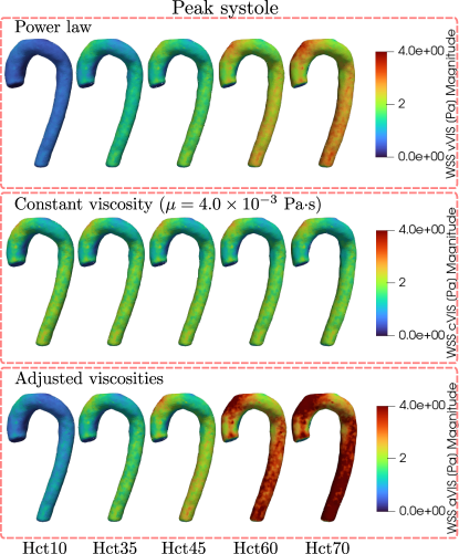
Figure 6: WSS maps at peak-systole estimated from simulated images for different Hct values. Estimations shown were obtained using power-law, Newtonian (0.004 $\text{Pa}\cdot\text{s}$), and fitted-Newtonian viscosities as outlined in Table 1.

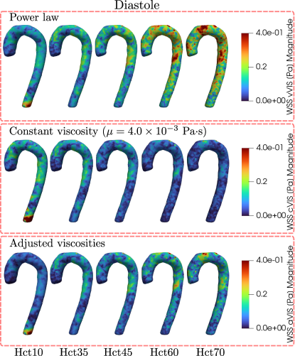
Figure 7: WSS maps at diastole estimated from simulated images for different Hct values. Estimations shown were obtained using power-law, Newtonian ($0.004~{}\text{Pa}\cdot\text{s}$), and fitted-Newtonian viscosities as outlined in Table 1.

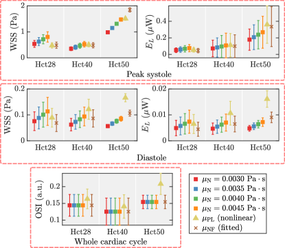
Figure 8: Mean values and standard deviation of WSS, OSI, and $E_{L}$ across four aortic segments obtained from in-vivo 4D Flow images. Estimations were made using Newtonian, fitted-Newtonian, and power-law viscosities. Remarkably, the results from these in-vivo experiments mirrored the trends observed in simulated images.

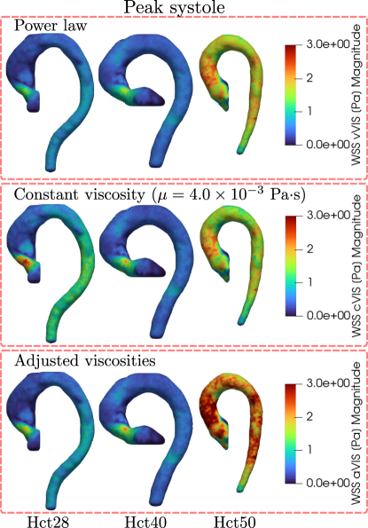
Figure 9: WSS maps at peak-systole estimated from in-vivo data for different Hct values. Estimations shown were obtained using power-law, Newtonian ($0.004~{}\text{Pa}\cdot\text{s}$), and fitted-Newtonian viscosities as outlined in Table 1.

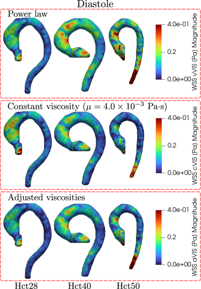
Figure 10: WSS maps at diastole estimated from in-vivo data for different Hct values. Estimations shown were obtained using power-law, Newtonian ($0.004~{}\text{Pa}\cdot\text{s}$), and fitted-Newtonian viscosities as outlined in Table 1.

5 Discussion

WSS estimated from noisy 4D Flow data demonstrated similar spatial distributions and variations with Hct levels compared to their CFD counterparts, as clearly shown in Figure S5, although a noticeable underestimation is made at peak systole. However, this underestimation align with previous studies, indicating that hemodynamic parameters, particularly WSS, are underestimated when using 4D Flow [60, 61, 57, 62, 63, 64, 65, 66]. Moreover, we observed the same behavior reported in [64] and [66]: WSS is highly underestimated at systole, and these differences are reduced at diastole. This gives us the confidence that all the estimations made from images are faithful representations of the ground-truth estimations derived from CFD simulations.

Results obtained from comparing the first and second scenarios described in the experiments section tested the need for a non-Newtonian model when computing relevant parameters such as those given in (3.1). The significance of this comparison arises from the possibility of using the Newtonian linear model as a surrogate for the power-law constitutive, which would eliminate the need for considering a nonlinear rheology. However, the differences observed in Figures 3, S6, and S7, show that both models are not interchangeable, similar, nor equivalent. Moreover, metrics such as WSS even change their behavior between systole and diastole, as the power-law (non-Newtonian) viscosity underestimates this parameter in diastole but overestimates it when compared with its fitted-Newtonian counterpart. This indicates that a constant viscosity (even when fitted for Hct levels) cannot characterize the flow dynamics through the whole cardiac cycle, as is also evident in OSI differences.

Results obtained from testing the third scenario also pointed in the same direction and clearly showed that Newtonian viscosities, whether fitted or not, do not allow the complete characterization of the cardiac cycle. A clear example can be seen by observing the trend in WSS for increasing Hct obtained with each model. Only WSS estimated using the power-law (see Figures 6 and 7) obtained the same variation with Hct as those obtained directly from CFD simulations (see Figures 9 and 10), despite the underestimation mentioned before.

Hemodynamic parameters obtained from in-vivo experiments exhibited similar trends to those obtained from simulations. However, despite the insightful and promising results, their interpretation must be carefully approached. This is due to several reasons: first, the limited number of data points (three) is insufficient for claiming definitive trends. Second, the range of Hct considered in the in-vivo experiments is smaller than that considered in the simulations, and third, the data was obtained from patients with different types of HCM. Therefore, it is a future endeavor of the authors to extend this study to a larger population, including healthy volunteers and patients with various diseases, to obtain trends and statistics that would be clinically meaningful.

The observed differences between estimations using the power-law, Newtonian, and fitted-Newtonian viscosities are noteworthy and warrant discussion. As highlighted earlier, hemodynamic parameters are often underestimated in 4D Flow MRI due to resolution-related imaging effects, specifically partial volume effects. This underestimation can be substantial, exceeding 50% of the ground-truth value during systole for a pixel size of 2 mm [66]. Therefore, it could be argued that such underestimations might impact the differences observed in the current investigation. However, it’s crucial to acknowledge that these underestimations are inherent in every 4D Flow-derived hemodynamic parameter. Despite this limitation, notable differences were observed in our study.

Regarding the current approach to estimating hemodynamic parameters, it is important to mention that due to the high variability in Newtonian viscosity values used in the literature, the statistics performed on viscosity-dependent parameters could be biased and might be limited for diagnostic purposes. Therefore, using a measurable criterion such as Hct to standardize the estimation of hemodynamic parameters would be a step forward.

A limitation of this investigation is the explicit unavailability of power-law parameters for a wide range of Hct at physiological temperature, e.g., 37^oC. In most of the literature reviewed for this work (see Table 1), only graphics with the adjusted curves were available, making the task of obtaining the values of $m$ and $n$ time-consuming. This underscores the necessity of standardizing blood rheology research by providing the parameters of the adjusted models and also the corresponding measurements.

All the previous discussions assumed that the Hct level is known for every patient at the moment of the 4D Flow exam. Although this assumption may not always be valid, it is not wrong to think that, in most cases, the data will be available, as the CBC is routinely performed in patients with heart failure and related comorbidities [67]. Additionally, CMR exams are often performed using gadolinium contrast agents, which cannot be administered to patients with severe renal impairment. Therefore, CBC to check renal function are often performed. Furthermore, this assumption is even more valid considering that CMR exams are typically performed last in the diagnostic pipeline primarily due to their elevated cost. However, this leads to a more complicated issue: is the CBC still valid at the moment of the 4D Flow exam?

Many efforts have been made to address this question in various contexts, including MRI. For instance, studies have shown that not only Hct but also several other hematological parameters can vary with posture [68], throughout the day [69, 70], and seasonally [71, 72, 73]. Other sources of variability include pre-analytical factors such as fasting condition, venous stasis, and exercise, which are usually standardized to reduce variation [73].

Considering these factors, the reported variations in Hct have been demonstrated not to affect the estimation of CMR-derived parameters directly dependent on Hct, such as extracellular volume [74]. Thus, we hypothesize that these variations would not induce significant differences in hemodynamic parameters estimated from 4D Flow data. However, this remains an open question.

6 Conclusion

Our study highlights the importance of recognizing the nonlinear behavior of blood when estimating hemodynamic parameters from 4D Flow MRI with available CBC data. The conventional use of Newtonian or fitted-Newtonian viscosities proves inadequate in capturing the intricate dynamics of blood flow, especially in major vessels like the aorta. In contrast, the power-law, a simple yet robust model, effectively represents the cardiac cycle’s dynamics, providing accurate estimations of key parameters such as WSS, $E_{L}$, and OSI. Its ease of integration into standard postprocessing frameworks enhances its practicality for researchers and clinicians.

7 Acknowledgments

HM, JS, and EC acknowledge the financial support given by ANID-FONDECYT through the projects Postdoctorado #3220266, Iniciación en Investigación #11200481, and Regular #1210156, respectively. JS also acknowledges to ANID-Millennium Science Initiative Program ICN2021004. FG acknowledges the funding PUCV Vinci DI-Iniciación 039.331/2023. We would like to kindly thank the Weierstraß-Institut für Angewandte Analysis und Stochastik (WIAS) for allowing the authors to run CFD simulations in their servers.

8 Supplementary Figures

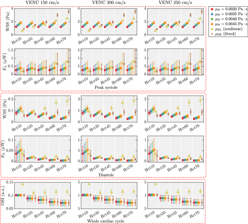
Figure 11: Mean values and standard-deviations of WSS, $E_{L}$, and OSI across aortic segments for different VENCs (i.e., different signal-to-noise ratios). Results are shown at peak systole and diastole. The figures indicate that almost no differences in hemodynamic parameters are induced with increasing VENC values as the signal-to-noise ratio worsens.

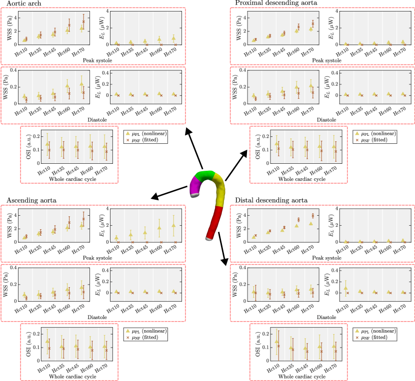
Figure 12: Mean values and standard deviations of WSS, $E_{L}$, and OSI for each aortic segment are estimated from simulated images obtained through CFD simulations with power-law and fitted-Newtonian viscosities. Results are presented at peak systole and diastole for a VENC of 250 cm/s. In each segment, the same trend for each hemodynamic parameter is observed, both in peak systole and diastole. Elevated standard deviations for WSS and $E_{L}$ are seen for an Hct of 10%, primarily due to the flow pattern depicted in Figure S6.

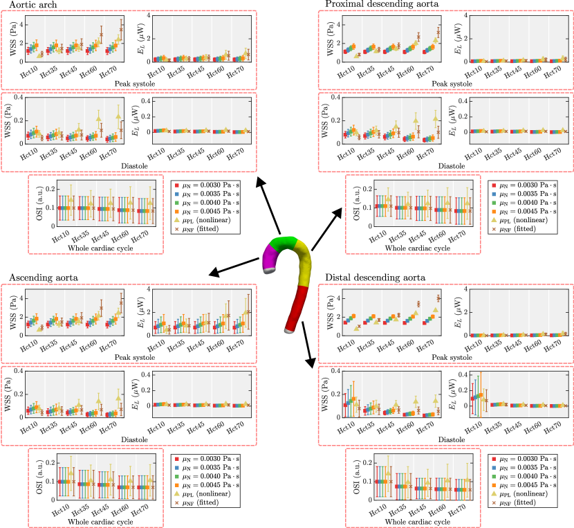
Figure 13: Mean values and standard deviations of WSS, $E_{L}$, and OSI estimated for each aortic segment from simulated images obtained through CFD simulations with nonlinear rheology. Results are presented at peak systole and diastole for a VENC of 250 cm/s. In each segment, the same trend for each hemodynamic parameter is observed, but with varying standard deviations, both in peak systole and diastole. Elevated standard deviations for WSS and $E_{L}$ are seen for an Hct of 10%, primarily due to the flow pattern depicted in Figure S6.

Figure 14: Mean values and standard deviations of WSS, $E_{L}$, and OSI estimated for each aortic segment from in-vivo 4D Flow images. Results are presented at peak systole and diastole. Similar trends are observed between segments in estimations made at peak systole. However, some variations in these trends are observed in diastole.

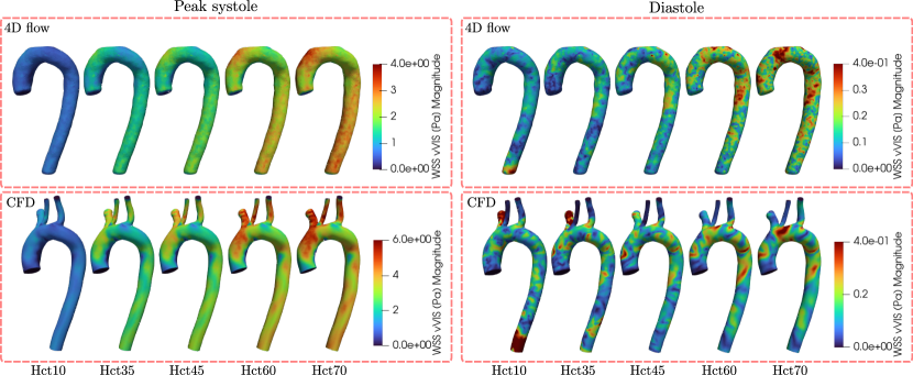
Figure 15: WSS maps at peak systole and diastole estimated from noisy simulated 4D Flow images and CFD simulations obtained using nonlinear rheology for different Hct values. The 4D Flow images were generated using a VENC of 250 cm/s. Color bars at peak systole have different ranges to show the spatial distributions of the maps clearly. Despite the noise level, the results reveal similar spatial variations between WSSs obtained from images and simulations at both peak systole and diastole. However, as reported in the literature, WSSs estimated from 4D Flow images underestimate their simulation counterparts.

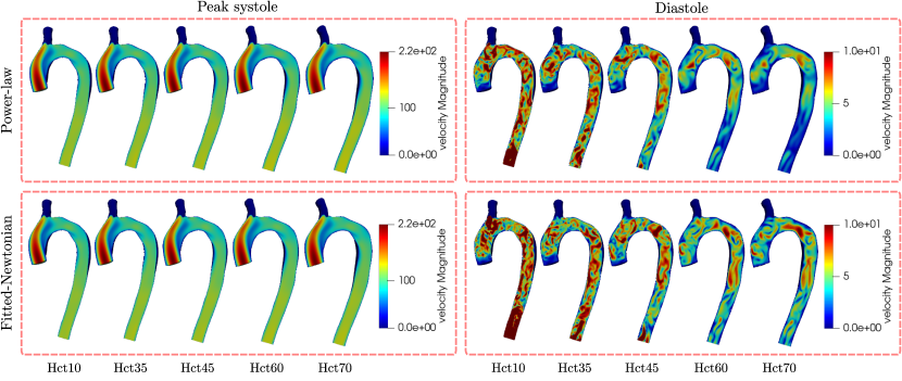
Figure 16: Velocity maps at peak systole and diastole extracted from CFD simulations obtained using power-law and fitted-Newtonian viscosities for different Hct values. Almost identical flow patterns are observed in peak systole, but differences are obtained in diastole.

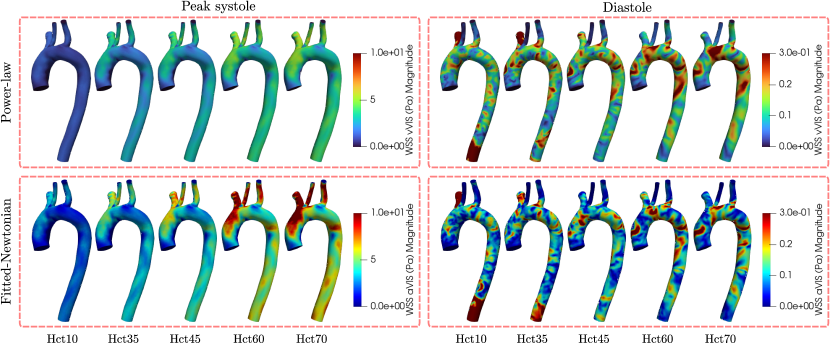
Figure 17: WSS maps at peak systole and diastole extracted from CFD simulations obtained using power-law and fitted-Newtonian viscosities for different Hct values. WSS obtained from the fitted viscosity simulations is greater in peak systole but smaller in diastole than those obtained using the power-law, indicating that both simulations cannot be used interchangeably.

References

- [1] Julio Sotelo, Pamela Franco, Andrea Guala, Lydia Dux-Santoy, Aroa Ruiz-Muñoz, Arturo Evangelista, Hernan Mella, Joaquín Mura, Daniel E. Hurtado, José F. Rodríguez-Palomares, and Sergio Uribe. Fully Three-Dimensional Hemodynamic Characterization of Altered Blood Flow in Bicuspid Aortic Valve Patients With Respect to Aortic Dilatation: A Finite Element Approach. Frontiers in Cardiovascular Medicine, 9, 2022.
- [2] John F. Jr. LaDisa, Ronak J. Dholakia, C. Alberto Figueroa, Irene E. Vignon-Clementel, Frandics P. Chan, Margaret M. Samyn, Joseph R. Cava, Charles A. Taylor, and Jeffrey A. Feinstein. Computational simulations demonstrate altered wall shear stress in aortic coarctation patients treated by resection with end-to-end anastomosis. Congenital Heart Disease, 6(5):432–443, 2011.
- [3] Emile S. Farag, Pim van Ooij, R. Nils Planken, Kayleigh C.P. Dukker, Frederiek de Heer, Berto J. Bouma, Danielle Robbers-Visser, Maarten Groenink, Aart J. Nederveen, Bas A.J.M. de Mol, Jolanda Kluin, and S. Matthijs Boekholdt. Aortic valve stenosis and aortic diameters determine the extent of increased wall shear stress in bicuspid aortic valve disease. Journal of Magnetic Resonance Imaging, 48(2):522–530, 2018.
- [4] K Takahashi, T Sekine, T Ando, Y Ishii, and S Kumita. Utility of 4d flow mri in thoracic aortic diseases: A literature review of clinical applications and current evidence. Magn Reson Med Sci, 21(2):327–339, September 2021.
- [5] Andreas Harloff, Andrea Nußbaumer, Simon Bauer, Aurélien F. Stalder, Alex Frydrychowicz, Cornelius Weiller, Jürgen Hennig, and Michael Markl. In vivo assessment of wall shear stress in the atherosclerotic aorta using flow-sensitive 4D MRI. Magnetic Resonance in Medicine, 63(6):1529–1536, 2010.
- [6] Erik T. Bieging, Alex Frydrychowicz, Andrew Wentland, Benjamin R. Landgraf, Kevin M. Johnson, Oliver Wieben, and Christopher J. François. In vivo three-dimensional MR wall shear stress estimation in ascending aortic dilatation. Journal of Magnetic Resonance Imaging, 33(3):589–597, 2011.
- [7] Pim van Ooij, Wouter V. Potters, Annetje Guédon, Joppe J. Schneiders, Henk A. Marquering, Charles B. Majoie, Ed vanBavel, and Aart J. Nederveen. Wall shear stress estimated with phase contrast MRI in an in vitro and in vivo intracranial aneurysm. Journal of Magnetic Resonance Imaging, 38(4):876–884, 2013.
- [8] AJ Barker, P van Ooij, K Bandi, J Garcia, M Albaghdadi, P McCarthy, RO Bonow, J Carr, J Collins, SC Malaisrie, and M Markl. Viscous energy loss in the presence of abnormal aortic flow. Magn Reson Med, 72(3):620–628, September 2014.
- [9] Jeremías Garay, Hernán Mella, Julio Sotelo, Cristian Cárcamo, Sergio Uribe, Cristóbal Bertoglio, and Joaquín Mura. Assessment of 4D flow MRI’s quality by verifying its Navier–Stokes compatibility. International Journal for Numerical Methods in Biomedical Engineering, 38(6):e3603, 2022.
- [10] Rick J. van Tuijl, Kimberley M. Timmins, Birgitta K. Velthuis, Pim van Ooij, Jaco J.M. Zwanenburg, Ynte M. Ruigrok, and Irene C. van der Schaaf. Hemodynamic Parameters in the Parent Arteries of Unruptured Intracranial Aneurysms Depend on Aneurysm Size and Are Different Compared to Contralateral Arteries: A 7 Tesla 4D Flow MRI Study. Journal of Magnetic Resonance Imaging, 59(1):223–230, 2024.
- [11] Prashanta Kumar Mandal. An unsteady analysis of non-Newtonian blood flow through tapered arteries with a stenosis. International Journal of Non-Linear Mechanics, 40(1):151–164, 2005.
- [12] Jessica Benitez Mendieta, Davide Fontanarosa, Jiaqiu Wang, Phani Kumari Paritala, Tim McGahan, Thomas Lloyd, and Zhiyong Li. The importance of blood rheology in patient-specific computational fluid dynamics simulation of stenotic carotid arteries. Biomechanics and Modeling in Mechanobiology, 19(5):1477–1490, 2020.
- [13] Frieke M.A. Box, Rob J. Van Der Geest, Marcel C.M. Rutten, and Johan H.C. Reiber. The influence of flow, vessel diameter, and non-Newtonian blood viscosity on the wall shear stress in a carotid bifurcation model for unsteady flow. Investigative Radiology, 40(5):277–294, 2005.
- [14] Sang Wook Lee and David A. Steinman. On the relative importance of rheology for image-based CFD models of the carotid bifurcation. Journal of Biomechanical Engineering, 129(2):273–278, 2007.
- [15] Hamidreza Gharahi, Byron A. Zambrano, David C. Zhu, J. Kevin DeMarco, and Seungik Baek. Computational fluid dynamic simulation of human carotid artery bifurcation based on anatomy and volumetric blood flow rate measured with magnetic resonance imaging. International Journal of Advances in Engineering Sciences and Applied Mathematics, 8(1):46–60, 2016.
- [16] Carolina Abugattas, Alejandro Aguirre, Ernesto Castillo, and Marcela Cruchaga. Numerical study of bifurcation blood flows using three different non-Newtonian constitutive models. Applied Mathematical Modelling, 88:529–549, 2020.
- [17] Takashi Suzuki, Hiroyuki Takao, Tomoaki Suzuki, Shunsuke Hataoka, Tomonobu Kodama, Ken Aoki, Katharina Otani, Toshihiro Ishibashi, Hideki Yamamoto, Yuichi Murayama, and Makoto Yamamoto. Proposal of hematocrit-based non-Newtonian viscosity model and its significance in intracranial aneurysm blood flow simulation. Journal of Non-Newtonian Fluid Mechanics, 290(February):1–11, 2021.
- [18] Roe E. Wells and Edward W. Merrill. Influence of flow properties upon viscosity-hematocrit relationships. The Journal of Clinical Investigation, 41(8):1591–1598, August 1962.
- [19] Frederick J. Walburn and Daniel J. Schneck. A constitutive equation for whole human blood. Biorheology, 13(3):201–210, January 1976.
- [20] Rym Mehri, Catherine Mavriplis, and Marianne Fenech. Red blood cell aggregates and their effect on non-Newtonian blood viscosity at low hematocrit in a two-fluid low shear rate microfluidic system. PLOS ONE, 13(7):e0199911, July 2018.
- [21] Milton Mendlowitz. The Effect of Anemia and Polycythemia on Digital Intravascular Blood Viscosity. The Journal of Clinical Investigation, 27(5):565–571, September 1948.
- [22] Sirisha Kundrapu and Jaime Noguez. Chapter Six - Laboratory Assessment of Anemia. In Gregory S. Makowski, editor, Advances in Clinical Chemistry, volume 83, pages 197–225. Elsevier, January 2018.
- [23] Henny H. Billett. Hemoglobin and Hematocrit. In H. Kenneth Walker, W. Dallas Hall, and J. Willis Hurst, editors, Clinical Methods: The History, Physical, and Laboratory Examinations. Butterworths, Boston, 3rd edition, 1990.
- [24] Lena Václavů, Zelonna A. V. Baldew, Sanna Gevers, Henri J. M. M. Mutsaerts, Karin Fijnvandraat, Marjon H. Cnossen, Charles B. Majoie, John C. Wood, Ed VanBavel, Bart J. Biemond, Pim van Ooij, and Aart J. Nederveen. Intracranial 4D flow magnetic resonance imaging reveals altered haemodynamics in sickle cell disease. British Journal of Haematology, 180(3):432–442, 2018.
- [25] Alessandra Riva, Francesco Sturla, Alessandro Caimi, Silvia Pica, Daniel Giese, Paolo Milani, Giovanni Palladini, Massimo Lombardi, Alberto Redaelli, and Emiliano Votta. 4D flow evaluation of blood non-Newtonian behavior in left ventricle flow analysis. Journal of Biomechanics, 119:110308, April 2021.
- [26] Catalina Farías, Camilo Bayona-Roa, Ernesto Castillo, Roberto C. Cabrales, and Ricardo Reyes. Reduced order modeling of parametrized pulsatile blood flows: Hematocrit percentage and heart rate. International Journal of Engineering Science, 193:103943, 2023.
- [27] Sarah Katz, Alfonso Caiazzo, and Volker John. Impact of viscosity modeling on the simulation of aortic blood flow. Journal of Computational and Applied Mathematics, 425:115036, June 2023.
- [28] Sabrina Lynch, Nitesh Nama, and C. Alberto Figueroa. Effects of non-Newtonian viscosity on arterial and venous flow and transport. Scientific Reports, 12(1):20568, November 2022.
- [29] Andrew L. Cheng, Choo Phei Wee, Niema M. Pahlevan, and John C. Wood. A 4D flow MRI evaluation of the impact of shear-dependent fluid viscosity on in vitro Fontan circulation flow. American Journal of Physiology-Heart and Circulatory Physiology, 317(6):H1243–H1253, December 2019.
- [30] Han Hung Yeh, Oleksandr Barannyk, Dana Grecov, and Peter Oshkai. The influence of hematocrit on the hemodynamics of artificial heart valve using fluid-structure interaction analysis. Computers in Biology and Medicine, 110:79–92, July 2019.
- [31] L. Formaggia, A. Quarteroni, and A. Veneziani. Cardiovascular Mathematics. Modeling and simulation of the circulatory system., volume 1. Springer, 01 2009.
- [32] D. Nolte and C. Bertoglio. Inverse problems in blood flow modeling: A review. International Jorunal for Numerical Methods in Biomedical Engineering, 2022.
- [33] F. Galarce, J.F. Gerbeau, D. Lombardi, and O. Mula. Fast reconstruction of 3D blood flows from Doppler ultrasound images and reduced models. Computer Methods in Applied Mechanics and Engineering, 375:113559, 2021.
- [34] Felipe Galarce, Damiano Lombardi, and Olga Mula. Reconstructing haemodynamics quantities of interest from doppler ultrasound imaging. International Journal for Numerical Methods in Biomedical Engineering, 37(2):e3416, 2021.
- [35] G. Arbia, I.E. Vignon-Clementel, T.-Y. Hsia, and J.-F. Gerbeau. Modified navier–stokes equations for the outflow boundary conditions in hemodynamics. European Journal of Mechanics - B/Fluids, 60:175–188, 2016.
- [36] Hernán Mella, Joaquín Mura, Julio Sotelo, and Sergio Uribe. A comprehensive comparison between shortest-path HARP refinement, SinMod, and DENSEanalysis processing tools applied to CSPAMM and DENSE images. Magnetic Resonance Imaging, 83:14–26, November 2021.
- [37] Hernan Mella, Joaquin Mura, Hui Wang, Michael D. Taylor, Radomir Chabiniok, Jaroslav Tintera, Julio Sotelo, and Sergio Uribe. HARP-I: A Harmonic Phase Interpolation Method for the Estimation of Motion from Tagged MR Images. IEEE Transactions on Medical Imaging, 40(4):1240–1252, 2021.
- [38] PyMRStrain, a Python library for the generation of synthetic MR strain phantoms. https://github.com/hmella/pymrstrain/tree/4dflow.
- [39] Nathan M. Wilson, Ana K. Ortiz, and Allison B. Johnson. The vascular model repository: A public resource of medical imaging data and blood flow simulation results. Journal of Medical Devices, 7(40923), 2013-12-05.
- [40] Martin R. Pfaller, Jonathan Pham, Aekaansh Verma, Luca Pegolotti, Nathan M. Wilson, David W. Parker, Weiguang Yang, and Alison L. Marsden. Automated generation of 0d and 1d reduced-order models of patient-specific blood flow. International Journal for Numerical Methods in Biomedical Engineering, 38(10):e3639, 2022.
- [41] Vascular Model Repository. https://www.vascularmodel.com/.
- [42] V. Jhon. Finite Element Methods for Incompressible Flow Problems. Springer, 2016.
- [43] F. Brezzi and J. Pitkaranta. On the stabilization of finite element approximations of the stokes equations. Efficient Solutions of Elliptic Systems, 1984.
- [44] Alexander N. Brooks and Thomas J.R. Hughes. Streamline upwind/petrov-galerkin formulations for convection dominated flows with particular emphasis on the incompressible navier-stokes equations. Computer Methods in Applied Mechanics and Engineering, 32(1):199–259, 1982.
- [45] T. E. Tezduyar. Stabilized Finite Element Formulations for Incompressible Flow Computations. In John W. Hutchinson and Theodore Y. Wu, editors, Advances in Applied Mechanics, volume 28, pages 1–44. Elsevier, January 1991.
- [46] A. González, R.C. Cabrales, and E. Castillo. Numerical study of the use of residual- and non-residual-based stabilized vms formulations for incompressible power-law fluids. Computer Methods in Applied Mechanics and Engineering, 400:115586, 2022.
- [47] R. Reyes, O. Ruz, C. Bayona-Roa, E. Castillo, and A. Tello. Reduced order modeling for parametrized generalized newtonian fluid flows. Journal of Computational Physics, 484:112086, 2023.
- [48] Mahdi Esmaily Moghadam, Yuri Bazilevs, Tain-Yen Hsia, Irene E. Vignon-Clementel, Alison L. Marsden, and Modeling of Congenital Hearts Alliance (MOCHA). A comparison of outlet boundary treatments for prevention of backflow divergence with relevance to blood flow simulations. Computational Mechanics, 48(3):277–291, September 2011.
- [49] Mahdi Esmaily Moghadam, Irene E. Vignon-Clementel, Richard Figliola, and Alison L. Marsden. A modular numerical method for implicit 0D/3D coupling in cardiovascular finite element simulations. Journal of Computational Physics, 244:63–79, July 2013.
- [50] F. Galarce Marin. Inverse problems in hemodynamics. Fast estimation of blood flows from medical data. https://gitlab.com/felipe.galarce.m/mad/. PhD thesis, INRIA Paris & Laboratoire Jacques-Louis Lions. Sorbonne Université, 2021.
- [51] S. Balay, S. Abhyankar, Adams. M.D., J. Brown, P. Brune, K. Buschelman, L. Dalcin, V. Eijkhout, W.D. Gropp, D. Kaushik, M.G. Knepley, L.C. McInnes, K. Rupp, B.F. Smith, S. Zampini, and H. Zhang. PETSc Web page, 2015.
- [52] M. Barth and E. Moser. Proton NMR relaxation times of human blood samples at 1.5 T and implications for functional MRI. Cellular and Molecular Biology (Noisy-Le-Grand, France), 43(5):783–791, July 1997.
- [53] Jacob A. Bender, Rizwan Ahmad, and Orlando P. Simonetti. The importance of k-space trajectory on off-resonance artifact in segmented echo-planar imaging. Concepts in Magnetic Resonance Part A: Bridging Education and Research, 42 A(2):23–31, March 2013.
- [54] Hannes Dillinger, Jonas Walheim, and Sebastian Kozerke. On the limitations of echo planar 4D flow MRI. Magnetic Resonance in Medicine, 84(4):1806–1816, 2020.
- [55] Malenka M. Bissell, Francesca Raimondi, Lamia Ait Ali, Bradley D. Allen, Alex J. Barker, Ann Bolger, Nicholas Burris, Carl-Johan Carhäll, Jeremy D. Collins, Tino Ebbers, Christopher J. Francois, Alex Frydrychowicz, Pankaj Garg, Julia Geiger, Hojin Ha, Anja Hennemuth, Michael D. Hope, Albert Hsiao, Kevin Johnson, Sebastian Kozerke, Liliana E. Ma, Michael Markl, Duarte Martins, Marci Messina, Thekla H. Oechtering, Pim van Ooij, Cynthia Rigsby, Jose Rodriguez-Palomares, Arno A. W. Roest, Alejandro Roldán-Alzate, Susanne Schnell, Julio Sotelo, Matthias Stuber, Ali B. Syed, Johannes Töger, Rob van der Geest, Jos Westenberg, Liang Zhong, Yumin Zhong, Oliver Wieben, and Petter Dyverfeldt. 4D Flow cardiovascular magnetic resonance consensus statement: 2023 update. Journal of Cardiovascular Magnetic Resonance, 25(1):40, July 2023.
- [56] 4d-flow-matlab-toolbox. https://github.com/JulioSoteloParraguez/4D-Flow-Matlab-Toolbox.
- [57] Julio Sotelo, Jesus Urbina, Israel Valverde, Cristian Tejos, Pablo Irarrazaval, Marcelo E. Andia, Sergio Uribe, and Daniel E. Hurtado. 3d quantification of wall shear stress and oscillatory shear index using a finite-element method in 3d cine pc-mri data of the thoracic aorta. IEEE Transactions on Medical Imaging, 35(6):1475–1487, January 2016.
- [58] Michael Loecher, Eric Schrauben, Kevin M. Johnson, and Oliver Wieben. Phase unwrapping in 4D MR flow with a 4D single-step laplacian algorithm. Journal of Magnetic Resonance Imaging, 43(4):833–842, 2016.
- [59] Kotomi Iwata, Tetsuro Sekine, Junya Matsuda, Masaki Tachi, Yoichi Imori, Yasuo Amano, Takahiro Ando, Makoto Obara, Gerard Crelier, Masashi Ogawa, Hitoshi Takano, and Shinichiro Kumita. Measurement of Turbulent Kinetic Energy in Hypertrophic Cardiomyopathy Using Triple-velocity Encoding 4D Flow MR Imaging. Magnetic Resonance in Medical Sciences, 23(1):39–48, 2024.
- [60] Sven Petersson, Petter Dyverfeldt, and Tino Ebbers. Assessment of the accuracy of MRI wall shear stress estimation using numerical simulations. Journal of Magnetic Resonance Imaging, 36(1):128–138, 2012.
- [61] Petter Dyverfeldt, Malenka Bissell, Alex J. Barker, Ann F. Bolger, Carl-Johan Carlhäll, Tino Ebbers, Christopher J. Francios, Alex Frydrychowicz, Julia Geiger, Daniel Giese, Michael D. Hope, Philip J. Kilner, Sebastian Kozerke, Saul Myerson, Stefan Neubauer, Oliver Wieben, and Michael Markl. 4D flow cardiovascular magnetic resonance consensus statement. Journal of Cardiovascular Magnetic Resonance, 17(1):72, August 2015.
- [62] Merih Cibis, Wouter V. Potters, Frank J. Gijsen, Henk Marquering, Pim van Ooij, Ed vanBavel, Jolanda J. Wentzel, and Aart J. Nederveen. The Effect of Spatial and Temporal Resolution of Cine Phase Contrast MRI on Wall Shear Stress and Oscillatory Shear Index Assessment. PLOS ONE, 11(9):e0163316, September 2016.
- [63] José Fernando Rodríguez-Palomares, Lydia Dux-Santoy, Andrea Guala, Raquel Kale, Giuliana Maldonado, Gisela Teixidó-Turà, Laura Galian, Marina Huguet, Filipa Valente, Laura Gutiérrez, Teresa González-Alujas, Kevin M. Johnson, Oliver Wieben, David García-Dorado, and Arturo Evangelista. Aortic flow patterns and wall shear stress maps by 4D-flow cardiovascular magnetic resonance in the assessment of aortic dilatation in bicuspid aortic valve disease. Journal of Cardiovascular Magnetic Resonance, 20(1):28, April 2018.
- [64] Jeremy Szajer and Kevin Ho-Shon. A comparison of 4D flow MRI-derived wall shear stress with computational fluid dynamics methods for intracranial aneurysms and carotid bifurcations — A review. Magnetic Resonance Imaging, 48:62–69, May 2018.
- [65] Edward Ferdian, David J. Dubowitz, Charlene A. Mauger, Alan Wang, and Alistair A. Young. WSSNet: Aortic Wall Shear Stress Estimation Using Deep Learning on 4D Flow MRI. Frontiers in Cardiovascular Medicine, 8, 2022.
- [66] Molly Cherry, Zinedine Khatir, Amirul Khan, and Malenka Bissell. The impact of 4D-Flow MRI spatial resolution on patient-specific CFD simulations of the thoracic aorta. Scientific Reports, 12(1):15128, September 2022.
- [67] Paul A. Heidenreich, Biykem Bozkurt, David Aguilar, Larry A. Allen, Joni J. Byun, Monica M. Colvin, Anita Deswal, Mark H. Drazner, Shannon M. Dunlay, Linda R. Evers, James C. Fang, Savitri E. Fedson, Gregg C. Fonarow, Salim S. Hayek, Adrian F. Hernandez, Prateeti Khazanie, Michelle M. Kittleson, Christopher S. Lee, Mark S. Link, Carmelo A. Milano, Lorraine C. Nnacheta, Alexander T. Sandhu, Lynne Warner Stevenson, Orly Vardeny, Amanda R. Vest, and Clyde W. Yancy. 2022 AHA/ACC/HFSA Guideline for the Management of Heart Failure: A Report of the American College of Cardiology/American Heart Association Joint Committee on Clinical Practice Guidelines. Circulation, 145(18):e895–e1032, May 2022.
- [68] Giris Jacob, Satish R. Raj, Terry Ketch, Boris Pavlin, Italo Biaggioni, Andrew C. Ertl, and David Robertson. Postural Pseudoanemia: Posture-Dependent Change in Hematocrit. Mayo Clinic Proceedings, 80(5):611–614, May 2005.
- [69] Henriette P. Sennels, Henrik L. Jørgensen, Anne-Louise S. Hansen, Jens P. Goetze, and Jan Fahrenkrug. Diurnal variation of hematology parameters in healthy young males: The Bispebjerg study of diurnal variations. Scandinavian Journal of Clinical and Laboratory Investigation, 71(7):532–541, November 2011.
- [70] Judith M. Hilderink, Lieke J. J. Klinkenberg, Kristin M. Aakre, Norbert C. J. de Wit, Yvonne M. C. Henskens, Noreen van der Linden, Otto Bekers, Roger J. M. W. Rennenberg, Richard P. Koopmans, and Steven J. R. Meex. Within-day biological variation and hour-to-hour reference change values for hematological parameters. Clinical Chemistry and Laboratory Medicine (CCLM), 55(7):1013–1024, July 2017.
- [71] Bernard E. Statland, Per Winkel, Steven C. Harris, Mary J. Burdsall, and Alex M. Saunders. Evaluation of Biologic Sources of Variation of Leukocyte Counts and Other Hematologic Quantities Using Very Precise Automated Analyzers. American Journal of Clinical Pathology, 69(1):48–54, January 1978.
- [72] M. Maes, S. Scharpé, W. Cooreman, A. Wauters, H. Neels, R. Verkerd, F. De Meyer, P. D’Hondt, D. Peeters, and P. Cosyns. Components of biological, including seasonal, variation in hematological measurements and plasma fibrinogen concentrations in normal humans. Experientia, 51(2):141–149, February 1995.
- [73] Poul Thirup. Haematocrit. Sports Medicine, 33(3):231–243, March 2003.
- [74] Mao-Yuan Su, Yu-Sen Huang, Emi Niisato, Kelvin Chow, Jyh-Ming Jimmy Juang, Cho-Kai Wu, Hsi-Yu Yu, Lian-Yu Lin, Shun-Chung Yang, and Yeun-Chung Chang. Is a timely assessment of the hematocrit necessary for cardiovascular magnetic resonance–derived extracellular volume measurements? Journal of Cardiovascular Magnetic Resonance, 22(1):77, November 2020.