Gradient Alignment with Prototype Feature for Fully Test-time Adaptation

Abstract

In context of Test-time Adaptation(TTA), we propose a regularizer, dubbed Gradient Alignment with Prototype feature (GAP), which alleviates the inappropriate guidance from entropy minimization loss from misclassified pseudo label. We developed a gradient alignment loss to precisely manage the adaptation process, ensuring that changes made for some data don’t negatively impact the model’s performance on other data. We introduce a prototype feature of a class as a proxy measure of the negative impact. To make GAP regularizer feasible under the TTA constraints, where model can only access test data without labels, we tailored its formula in two ways: approximating prototype features with weight vectors of the classifier, calculating gradient without back-propagation. We demonstrate GAP significantly improves TTA methods across various datasets, which proves its versatility and effectiveness.

1 Introduction

Deep learning models have achieved remarkable success, largely predicated on the assumption that training and test data are drawn from the same distribution Krizhevsky et al. (2017). However, this assumption often fails to hold true in real-world scenarios, where variables like weather changes and natural corruptions, such as rain, snow, or lens spots, can significantly alter data distributions. These distribution shifts expose the vulnerability of conventional deep learning models, leading to performance degradation when faced with such natural corruptions Hendrycks and Dietterich (2019).

To address the challenge of unknown distribution shifts, various approaches have been developed, including Domain Adaptation (DA) Csurka (2017), Domain Generalization (DG) Muandet et al. (2013), Unsupervised Domain Adaptation (UDA) Ganin and Lempitsky (2015), and Source-Free Domain Adaptation (SFDA) Liang et al. (2020); Lee et al. (2022). These methods, however, typically require access to training data or a dedicated stage to adapt the model to test data, which may not be feasible in many real-world applications due to constraints like the unavailability of training data or the impracticality of allocating extensive time to adaptation.

This gap in practical application has led to the emergence of Test-time Adaptation (TTA) Wang et al. (2021). TTA focuses on adapting a model during the inference phase, using only the test data that is streamed online, without access to training data or test labels. Common strategies employed in TTA include objectives like entropy minimization Wang et al. (2021) or cross-entropy with pseudo-labels Goyal et al. (2022), designed to guide the model’s self-supervision. However, these methods are susceptible to confirmation bias Arazo et al. (2020), where data with noisy predictions can lead the model to continually learn in the wrong direction.

To address this challenge, our approach focuses on adapting to new data while concurrently evaluating its impact on other data, effectively integrating prior knowledge into the adaptation process. We introduce a novel regularizer, named Gradient Alignment with Prototype feature (GAP), designed to ensure that adaptations made on data from a specific class do not negatively impact predictions for other data within the same class. GAP regularizer employs the concept of a prototype feature as an indirect metric to represent the prediction quality over data in a given class. Thus, its objective is designed to boost the prediction quality of the data from the same class and is implemented to boost that of prototype after adaptation.

To measure the change in the loss for the prototype feature, we employ a first-order Taylor expansion. The resulting objective is to maximize the dot product between the gradients of the prototype and the test data. Given TTA constraints, such as the lack of test labels, we have reformulated the GAP regularizer for practical application. For a representative yet computationally manageable prototype feature, we utilize the classifier’s weights in the fully-connected layer as a proxy. To enable computationally efficient sample-wise gradient calculation, we have developed a method to calculate the gradient for these weights using the results from the forward pass, thereby eliminating the need for back-propagation.

Our extensive experiments on public TTA benchmark datasets, including CIFAR-10-C and ImageNet-C Hendrycks and Dietterich (2019), as well as on large-scale and domain-shifted datasets like ImageNet-3DCC Kar et al. (2022), ImageNet-R Hendrycks et al. (2021), and VISDA-2021 Bashkirova et al. (2022), demonstrate the robustness and effectiveness of the GAP regularizer. We show that GAP not only improves model accuracy on corrupted or domain-shifted data but also aligns with the practical constraints of TTA, achieving consistent performance improvements across various datasets and baseline methods.

Our contributions are summarized as follows:

• We present the Gradient Alignment with Prototype Feature (GAP) regularizer, a new method that effectively handles changes in data during test-time adaptation. It uses a concept called prototype feature to gauge how well the model predicts, helping to overcome common biases and ensuring the model adapts well to new data without affecting its accuracy on existing classes.

• Our method is not just theoretically sound but also aligns well with the practical constraints of TTA, such as the unavailability of training data and the need for computational efficiency. This makes GAP an adaptable and feasible solution for real-world applications facing domain shift challenges.

• We validate the effectiveness of the GAP regularizer through extensive experiments on a range of public benchmark datasets, including CIFAR-10-C, ImageNet-C, ImageNet-3DCC, ImageNet-R, and VISDA-2021. These experiments not only demonstrate the robustness of our method but also its versatility across different types of data and baseline methods.

2 Related Work

2.0.1 Test-Time Adaptation (TTA)

TTA is a task that performs inference while adapting to an online test data stream, without access to the training data. It shares a similar paradigm with source-free domain adaptation (SFDA) Liang et al. (2020), in which that training data is inaccessible. While SFDA performs adaptation before actual inference, TTA requires on-the-fly adaptation during inference time. To meet the tight computation constraints, NORM  Schneider et al. (2020) updates only the batch normalization statistics on mini-batch samples during test time. Furthermore, labels of the test data are absent in the TTA context, so augmentation methods or unsupervised losses are employed for the TTA task. TTT Sun et al. (2020), MEMO Zhang et al. (2022), Test-time Augmentation Ashukha et al. (2020), and DUA Mirza et al. (2022) require augmented images of the test data. There are two main types of unsupervised losses in TTA: the entropy minimization loss and the cross-entropy loss with pseudo-labels. TENT Wang et al. (2021) and EATA Niu et al. (2022) optimize entropy minimization loss while adapting batch normalization statistics during test time. PL Lee and others (2013) generates pseudo-labels based on model predictions and uses cross-entropy loss to adapt the batch normalization layer parameters to the test data. Our proposed GAP loss is generic enough to be integrated with different TTA methods.

2.0.2 Gradient Alignment

Gradient alignment techniques are gaining momentum in domain adaptation and generalization, presenting innovative solutions to domain shift challenges. Gao et al. (2021) developed Feature Gradient Distribution Alignment (FGDA) for adversarial domain adaptation, which aims at aligning feature gradients to improve error bounds for target samples. In the field of domain generalization, Shi et al. (2021) introduced an inter-domain gradient matching method. To overcome the computational burden of direct gradient inner product optimization, they devised a simpler first-order algorithm called Fish. In medical imaging,  Zeng et al. (2022) applied gradient matching in Gradient Matching Federated Domain Adaptation (GM-FedDA) for brain image classification in federated learning settings. These methods strive to minimize gradient discrepancies across domains, tackling computational complexity and overfitting risks, thus underscoring the practical value of gradient techniques in domain adaptation and generalization. Our method avoids the need for heavy second-order derivatives required for direct application of GAP. We have redesigned it to fit efficiency-centric Test-Time Adaptation (TTA) scenarios, allowing calculations solely through forward passes, making it a more streamlined and efficient solution.

3 Proposed Method

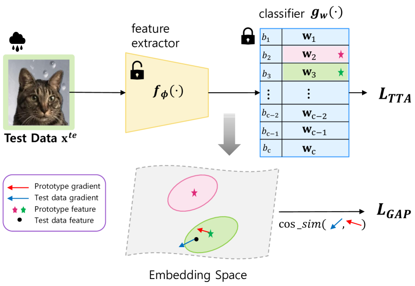
Figure 1: Overview of Gradient Alignment with Prototype feature for TTA. First, we compute and store the gradients of weights. Next, we conduct inference and determine the pseudo-label for the test data for weighting strategy. Finally, we calculate the GAP regularizer which increases the cosine similarity between the gradient of the weight and gradient of the test data.

3.1 Preliminaries

The training data is denoted as $\mathcal{D}_{\mathrm{tr}}=\{(\mathbf{x}_{i}^{tr},y_{i}^{tr}):\mathbf{x}_{i}^{tr}\sim P(\mathcal{X})\text{ and }y_{i}^{tr}\in\mathcal{Y}\}_{i=1}^{N_{\mathrm{train}}}$. The test data is denoted as $\mathcal{D}_{\mathrm{te}}=\{(\mathbf{x}_{i}^{te},y_{i}^{te}):\mathbf{x}_{i}^{te}\sim Q(\mathcal{X})\text{ and }y_{i}^{te}\in\mathcal{Y}\}_{i=1}^{N_{\mathrm{test}}}$. In TTA setting, $P(\mathcal{X})\neq Q(\mathcal{X})$ and we cannot access $y_{i}^{te}$. The training data and test data share the same label space $\mathcal{Y}=\{1,2,\dots,c\}$ with $c$ distinct classes. Let’s assume the model is structured with a feature extractor and a classifier. Here, $f_{\bm{\phi}}:\mathcal{X}\rightarrow\mathcal{Z}$ represents the pretrained feature extractor, where $\mathcal{Z}$ is the embedding space, and $\bm{\phi}$ is the parameter of the feature extractor. The pretrained classifier denoted as $g_{\bm{w}}:\mathcal{Z}\rightarrow\mathbb{R}^{c}$, consisting of a single fully-connected layer, where $\bm{w}=\{\mathbf{b},\mathbf{w}_{1},\mathbf{w}_{2},\ldots,\mathbf{w}_{c}\}$. The loss function is defined as $l:\mathbb{R}^{c}\rightarrow\mathbb{R}$.
During adaptation, test data are provided online. At time step $t$, the model receives the test data $\mathbf{x}^{te}_{i}$ as input, making prediction $(g_{\bm{w}_{t}}\circ f_{\bm{\phi}_{t}})(\mathbf{x}^{te}_{i})$. It then adjusts itself for subsequent inputs, updating $\bm{\phi}_{t},\bm{w}_{t}\rightarrow\bm{\phi}_{t+1},\bm{w}_{t+1}$ guided by the loss function.
At each time step, we define prototype features for each class in the embedding space $\mathcal{Z}$. Let’s denote the set of prototype features as $P_{t}=\{\mathbf{p}_{1}^{t},\mathbf{p}_{2}^{t},\cdots,\mathbf{p}_{c}^{t}\}$. The element $\mathbf{p}^{t}_{k}$ is prototype feature, corresponding to a specific class $k$.

3.2 GAP: Gradient Alignment with Prototype Feature

We propose a regularizer designed to ensure that adaptation with data from a specific class does not compromise the prediction quality for other data within that class. To approximate the prediction quality for a given class, we introduce the concept of a prototype feature for the class, as an indirect metric. To be specific, we optimize $\bm{w}_{t}$ with respect to test data $\mathbf{x}^{te}_{i}$ at time step $t$. The objective of the regularizer is to maximize the reduction in loss associated with the prototype feature $\mathbf{p}_{k}^{t}$. Here, $l(\mathbf{p}_{k}^{t};\bm{w}_{t})$ represents the loss $l(g_{\bm{w}_{t}}(\mathbf{p}_{k}^{t}))$.

$$\Delta l(\mathbf{p}_{k}^{t})=l(\mathbf{p}_{k}^{t};\bm{w}_{t})-l(\mathbf{p}_{k}^{t};\bm{w}_{t+1})$$ (1)

The feature of the test data $\mathbf{x}^{te}_{i}$ is represented as $\mathbf{z}^{te}_{i}=f_{\bm{\phi}_{t}}(\mathbf{x}^{te}_{i})$. The parameters are updated using gradient descent, as described by the following equation:

$$\bm{w}_{t+1}=\bm{w}_{t}-\alpha_{t}\frac{d\,l(\mathbf{z}^{te}_{i};\bm{w})}{d\bm{w}}\Bigg{|}_{\bm{w}=\bm{w}_{t}}$$ (2)

where $\alpha_{t}>0$ is the learning rate at time step $t$.
The derivative of $\bm{w}_{t+1}$ with respect to $\alpha_{t}$ is given as follows:

$$\frac{dw_{t+1}}{d\alpha_{t}}=-\frac{d\,l(\mathbf{z}^{te}_{i};\bm{w})}{d\bm{w}}\Bigg{|}_{\bm{w}=\bm{w}_{t}}=-\nabla_{\bm{w}}l(\mathbf{z}^{te}_{i};\bm{w}_{t})$$ (3)

The first-order Taylor expansion of $l(\mathbf{p}_{k}^{t};\bm{w}_{t+1})$ around $\alpha_{t}=0$ gives

$$l(\mathbf{p}_{k}^{t};\bm{w}_{t+1})\approx l(\mathbf{p}_{k}^{t};\bm{w}_{t})+\alpha_{t}\times\frac{d\,l(\mathbf{p}_{k}^{t};w_{t+1})}{d\alpha_{t}}\Bigg{|}_{\alpha_{t}=0}$$ (4)

since $\bm{w}_{t+1}=\bm{w}_{t}$ when $\alpha_{t}=0$.
Substituting Equation 4 into $\Delta l(\mathbf{p}_{k}^{t})$ and applying the chain rule, along with the use of Equation 3, we obtain the following expression:

$$\Delta l(\mathbf{p}_{k}^{t}) \approx-\alpha_{t}\times\frac{d\,l(\mathbf{p}_{k}^{t};w_{t+1})}{d\alpha_{t}}\Bigg{|}_{\alpha_{t}=0}$$ (5)

$$=-\alpha_{t}\times\nabla_{\bm{w}}l(\mathbf{p}^{t}_{k};\bm{w}_{t})^{T}\frac{dw_{t+1}}{d\alpha_{t}}\Bigg{|}_{\alpha_{t}=0}$$ (6)

$$=\alpha_{t}\times\nabla_{\bm{w}}l(\mathbf{p}^{t}_{k};\bm{w}_{t})^{T}\nabla_{\bm{w}}l(\mathbf{z}^{te}_{i};\bm{w}_{t})$$ (7)

Our objective is to maximize $\Delta l(\mathbf{p}_{k}^{t})$ . Since gradient descent assumes $\alpha_{t}$ to be positive, maximizing $\Delta l(\mathbf{p}_{k}^{t})$ is equivalent to maximizing $\nabla_{\bm{w}}l(\mathbf{p}^{t}_{k};\bm{w}_{t})^{T}\nabla_{\bm{w}}l(\mathbf{z}^{te}_{i};\bm{w}_{t})$ which is dot product of two gradients.

3.2.1 Weighting Strategy

Adapting to $\mathbf{x}_{te}$ does not uniformly affect all classes. To address this, we introduce a weighting function, which determines the extent of influence to be assigned to each class prototype. A common weighting approach is to use pseudo-label of $\mathbf{z}^{te}_{i}$. The pseudo-label of $\mathbf{z}^{te}_{i}$ is denoted as $h(\mathbf{z}^{te}_{i})$. $h(\mathbf{z}^{te}_{i})$ can be either hard or soft. The weighted GAP regularizer is:

$$\mathcal{L}_{\text{GAP}}=-\sum_{k=1}^{c}h(\mathbf{z}^{te}_{i})_{k}\nabla_{\bm{w}}l(\mathbf{p}^{t}_{k};\bm{w}_{t})^{T}\nabla_{\bm{w}}l(\mathbf{z}^{te}_{i};\bm{w}_{t})$$ (8)

3.3 Feasible Implementation of GAP for TTA

In the TTA setting, two significant constraints are imposed. First, the model can only access data from the current mini-batch, not the entire dataset, and this mini-batch data is unlabeled. This makes it infeasible to obtain prototype features at each time step. Second, the adaptation algorithm must be efficient in terms of both computation and memory usage, as it is required to operate during inference time. The GAP regularizer necessitates instance-wise gradients. A straightforward approach to achieve this would be to perform back-propagation for each sample individually. However, such a method would substantially increase the computational load, which is not feasible in the context of Test-Time Adaptation (TTA). In this section, we present two strategies specifically designed to address the aforementioned challenges.

3.3.1 Approximation for Prototype Features

We adopt the classifier weights as proxies for prototype features. Since the model’s classifier is responsible for mapping features to their respective classes Snell et al. (2017), we treat each weight vector in the classifier as a representative prototype feature for that class.

$$\mathbf{p}_{k}^{t}\approx\mathbf{w}_{k}^{t}$$ (9)

3.3.2 Efficient Computation for GAP

In TTA setting, we usually update only batch normalization (BN) layers for stability and efficiency Wang et al. (2021). Therefore we fix the classifier and update only BN layers within the feature extractor. Consequently,$\mathbf{w}_{k}^{t}=\mathbf{w}_{k}^{t_{0}}=\mathbf{w}_{k}$.
Computing gradients with respect to $\bm{w}$ can be demanding in terms of memory and time. To address this, we focus on calculating gradients solely for the classifier’s $m$-th weight, determined by the hard pseudo-label $m={\operatorname*{argmin}}_{j\in\mathcal{Y}}g_{\bm{w}_{t}}(\mathbf{z}^{te}_{i})_{j}$ of the test data.
Furthermore, we maximize cosine similarity between the gradients rather than their dot product for the stability of our model.
The final GAP regularizer for test data $\mathbf{x}_{i}^{te}$ can be expressed as follows:

$$\mathcal{L}_{\text{GAP}}=-\sum_{k=1}^{c}h(\mathbf{z}^{te}_{i})_{k}\mathrm{cos\_sim}[\nabla_{\mathbf{w}_{m}}l(\mathbf{w}_{k};\bm{w}),\nabla_{\mathbf{w}_{m}}l(\mathbf{z}^{te}_{i};\bm{w})]$$ (10)

The GAP regularizer is versatile, compatible with various loss functions. In TTA scenarios, where labels are absent and efficiency is crucial, we opt for entropy minimization (EM) loss and cross-entropy (CE) loss with pseudo-labels as suitable choices. We have reformulated the EM/CE loss, enabling the calculation of the gradient with respect to the classifier’s weight through a single forward pass.
EM loss is given by:

$$l_{EM}(z;\bm{w})\coloneqq l_{EM}(g_{\bm{w}}(\mathbf{z}))=-\sum_{j=1}^{c}g_{\bm{w}}(\mathbf{z})_{j}\log g_{\bm{w}}(\mathbf{z})_{j}$$ (11)

The gradient of the EM loss is given by:

$$\nabla_{\mathbf{w}_{k}}l_{EM}(\mathbf{z};\bm{w})=\mathbf{z}\cdot\left(-\frac{g_{\bm{w}}(\mathbf{z})_{k}}{S}-C\right)$$ (12)

where $C=g_{\bm{w}}(\mathbf{z})\cdot\exp(g_{\bm{w}}(\mathbf{z}))$ and $S=\sum_{j=1}^{c}\exp(g_{\bm{w}}(\mathbf{z}))_{j}$.
CE loss with pseudo-label is given by:

$$l_{CE}(z;\bm{w})\coloneqq l_{CE}(g_{\bm{w}}(\mathbf{z}))=-\sum_{j=1}^{c}h(\mathbf{z})_{j}\log g_{\bm{w}}(\mathbf{z})_{j}$$ (13)

The gradient of the CE loss is given by:

$$\nabla_{\mathbf{w}_{k}}l_{CE}(\mathbf{z};\bm{w})=\mathbf{z}\cdot(g_{\bm{w}}(\mathbf{z})_{k}-h(\mathbf{z})_{k})$$ (14)

where $h(\mathbf{z})$ is pseudo-label of $z$.
Considering that the classifier is fixed during adaptation, $\nabla_{\mathbf{w}_{k}}l(\mathbf{w}_{k};\bm{w})$ is a pre-computable value before adaptation.
Finally, the model update the parameter of the BN layers by following objectives.

$$\mathcal{L}_{\text{total}}=\mathcal{L}_{\text{TTA}}+\beta\mathcal{L}_{\text{GAP}}.$$ (15)

Here, $\mathcal{L}_{\text{TTA}}$ refers to any TTA loss function, and $\beta$ is a hyper-parameter that determines the weight of the GAP regularizer. We scheduled the coefficient, $\beta$, of the regularizer to follow a simple exponential decay function. The algorithm for the GAP regularizer is outlined below:

Result: Test-time adapted model

Input: Pre-trained model, test data $\mathcal{D}_{\mathrm{te}}=\{\mathbf{x}_{i}^{te}\}_{i=1}^{N_{\mathrm{test}}}$

Calculate and save gradient of weight

$\{\nabla_{\mathbf{w}_{1}}l(\mathbf{w}_{1};\bm{w}),\cdots\nabla_{\mathbf{w}_{c}}l(\mathbf{w}_{c};\bm{w})\}$.

for a batch $B=\{\mathbf{x}_{b}^{te}\}_{b=1}^{B}\subset\mathcal{D}_{\mathrm{te}}$ do

       Update batch norm statistics using B

      Perform inference by calculating $(g_{\bm{w}_{t}}\circ f_{\bm{\phi}_{t}})(B)$.

      Calculate $\mathcal{L}_{\text{GAP}}(B)$ using Equation 10

      Update parameters of BN layer using Equation 15

end for

Algorithm 1 Gradient Alignment with Prototype feature

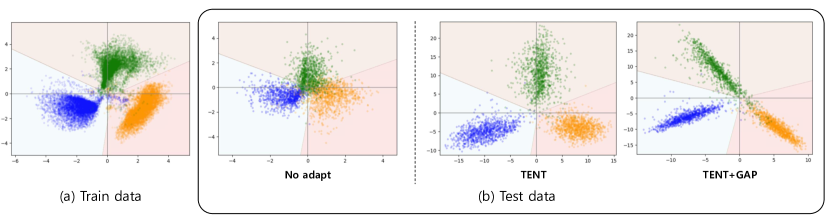
Figure 2: Conceptual Demonstration for GAP: (a) features plot of the training dataset, MNIST. (b) features plot of the test dataset, MNIST-C with dotted lines. We visualize features that were not used for adaptation.

Method	Gauss.	Shot	Impul.	Defoc.	Glass	Motion	Zoom	Snow	Frost	Fog	Brit.	Contr.	Elastic	Pixel	JPEG	AVG $\uparrow$
No adapt	27.7	34.3	27.1	53.1	45.7	65.3	58.0	74.9	58.7	74.0	90.7	53.3	73.4	41.6	69.7	56.5
Norm	71.5	73.7	63.9	87.1	64.8	86.1	87.8	82.5	82.2	84.8	91.6	86.7	76.4	80.1	72.3	79.4
PL	73.4	74.7	65.8	87.3	66.7	85.9	87.9	83.1	82.5	85.2	91.5	87.8	76.8	81.2	73.9	80.2
+GAP	77.5±0.2	80.0±0.1	71.1±0.1	88.8±0.1	70.6±0.3	87.7±0.2	89.6±0.2	85.6±0.4	85.1±0.1	87.6±0.4	92.2±0.0	89.6±0.4	79.0±0.5	84.5±0.2	78.0±0.0	83.1±0.0($+2.9$)
TENT	75.2	77.6	68.0	87.9	68.2	86.7	89.0	83.9	83.6	86.2	91.8	88.4	78.0	82.9	75.7	81.5
+GAP	77.5±0.2	80.0±0.2	71.1±0.2	88.8±0.1	70.7±0.3	87.7±0.3	89.6±0.1	85.7±0.3	85.2±0.0	87.6±0.3	92.2±0.1	89.7±0.3	79.2±0.3	84.5±0.2	78.3±0.2	83.2±0.0($+1.7$)
EATA	75.4	78.1	68.3	87.9	69.0	86.9	89.2	84.4	83.7	86.7	91.9	88.8	78.4	83.4	76.0	81.9
+GAP	78.0±0.1	80.5±0.1	71.6±0.3	89.1±0.1	71.3±0.1	88.0±0.2	89.8±0.0	85.9±0.3	85.5±0.1	87.8±0.1	92.2±0.1	89.8±0.2	79.7±0.1	85.0±0.0	78.9±0.5	83.5±0.0($+1.6$)

Table 1: Classification Accuracy (%) for each corruption in CIFAR-10-C at the highest severity (Level 5). We use WRN-28-10. Higher accuracy is shown in bold. The numbers written in red indicate the extent of performance improvement.

4 Experiments

4.1 Setup

4.1.1 Datasets

We conducted experiments on five datasets, which included two widely recognized TTA benchmark datasets: CIFAR-10-C and ImageNet-C Hendrycks and Dietterich (2019). Additionally, we included three large-scale datasets in our study: ImageNet-3DCC Kar et al. (2022), ImageNet-R Hendrycks et al. (2021), and VISDA-2021 Bashkirova et al. (2022).

Both CIFAR-10-C and ImageNet-C consist of corrupted images, each featuring 15 distinct corruption types with five levels of severity. The ImageNet 3D Common Corruptions (ImageNet-3DCC) dataset introduces 3D geometry-aware transformations to produce more realistic corruptions, offering 12 unique corruption types, each with five severity levels. In our experiments involving these three datasets, we focused specifically on level-5 severity, the most extreme form of corruption.

Complementing these, ImageNet-R and VISDA-2021 serve as benchmark datasets for domain shift. They comprise a diverse range of distributions, sourced from various style domains such as cartoons and sketches. This domain shift poses a greater challenge for model adaptation compared to image corruptions.

4.1.2 Architectures

For the CIFAR-10-C benchmark, our base model, pretrained on an uncorrupted dataset, is a Wide-ResNet-28-10 Zagoruyko and Komodakis (2016). For the other datasets, our base model is a ResNet-50 with a batch normalization(BN) layer He et al. (2016), pretrained on ImageNet Russakovsky et al. (2015).

4.1.3 Baseline Methods

We evaluate the performance improvement achieved by applying the GAP regularizer to the baseline methods described below.

• No adapt evaluates performance of the pretrained model without any adaptation.

• NORM Schneider et al. (2020) updates the BN statistics on the mini-batch samples during test time.

• PL Lee and others (2013) generates a one-hot pseudo-label based on the model’s prediction and applies cross-entropy loss to adjust BN parameters according to the test data.

• TENT Wang et al. (2021) updates the statistics and parameters of BN layer by employing an entropy minimization loss.

• EATA Niu et al. (2022) employs the Fisher regularizer to safeguard crucial parameter stability and conducts instance selection and re-weighting as part of entropy minimization loss.

• SAR Niu et al. (2023) removes partial noisy samples with large gradients and use reliable entropy minimization methods.

• DEYO Anonymous (2024) uses a novel confidence metric named Pseudo-Label Probability Difference (PLPD) to filter out noisy samples.

4.1.4 Implementation Details

For the CIFAR-10-C, we employ the pretrained model weights derived from the official implementations of TENT, adhering to the RobustBench protocol Croce et al. (2020). We set the batch size to 128 and follow the implementation details used in TENT, utilizing an NVIDIA GeForce RTX 3090 Ti GPU. For the ImageNet-C and ImageNet-3DCC dataset, we reference the base code from SAR and EATA, following the implementation details provided in each paper. We set the batch size to 64 and employ an NVIDIA A40 GPU. For the ImageNet-R and VISDA-2021 dataset, we reference the base code from DEYO. We set the batch size to 64 and employ an NVIDIA A40 GPU. We report the average performance based on three different random seeds for all experiments.

We implement a hard pseudo-label approach as the weighting strategy for the GAP regularizer. For the calculation of both the prototype gradient and the test data gradient, we employ the Entropy Minimization (EM) loss.

The GAP regularizer is governed by two hyper-parameters: $\beta$ and $\gamma$. The parameter $\beta$ sets the initial weight of the GAP regularizer. Specifically, we assign $\beta=100$ for the CIFAR-10-C dataset, $\beta=20$ for ImageNet-C dataset with DEYO, and $\beta=10$ for ImageNet-3DCC dataset with EATA. For all other experiments, $\beta$ is set to 50. The parameter $\gamma$ determines the decay rate of the exponential decay function, defined as $y=\exp[-\frac{t}{\gamma}]$. This function progressively reduces the influence of the GAP regularizer, where a larger $\gamma$ value indicates a slower decay. Specifically, for the CIFAR-10-C dataset, we set $\gamma=500$, while for other datasets, $\gamma$ is set to 100.

Method	Gauss.	Shot	Impul.	Defoc.	Glass	Motion	Zoom	Snow	Frost	Fog	Brit.	Contr.	Elastic	Pixel	JPEG	AVG $\uparrow$
No adapt	2.2	2.9	1.8	17.9	9.8	14.8	22.5	16.9	23.3	24.4	58.9	5.4	16.9	20.6	31.7	18.0
Norm	15.2	15.8	15.8	15.0	15.4	26.3	38.9	34.3	33.0	48.0	65.2	16.9	44.1	49.0	39.8	31.5
PL	25.8	27.5	26.9	25.2	24.5	37.8	47.2	44.3	39.3	55.8	66.9	24.8	52.3	56.7	49.9	40.3
+GAP	28.5±0.4	30.0±0.3	30.3±0.2	28.4±0.5	27.4±0.3	42.2±0.3	49.6±0.2	48.0±0.2	41.9±0.2	58.1±0.1	67.5±0.1	31.3±0.5	55.3±0.1	59.1±0.0	52.9±0.1	43.4±0.0($+3.1$)
TENT	28.6	30.6	30.0	28.0	27.1	41.3	49.2	47.2	40.9	57.6	67.4	26.1	54.7	58.5	52.2	42.6
+GAP	30.2±0.3	31.8±0.2	31.9±0.2	29.7±0.1	28.9±0.1	43.7±0.1	50.4±0.1	49.1±0.1	42.3±0.1	58.5±0.1	67.6±0.1	30.7±1.2	56.0±0.1	59.6±0.0	53.5±0.1	44.2±0.1($+1.6$)
EATA	34.8	37.0	35.7	33.5	33.2	46.8	52.8	51.6	45.7	60.0	68.1	44.5	57.9	60.5	55.1	47.8
+GAP	35.4±0.5	38.1±0.2	36.7±0.8	33.8±0.9	33.9±0.3	48.6±0.2	53.1±0.0	52.8±0.2	46.5±0.2	60.5±0.1	67.6±0.1	46.0±0.6	58.5±0.1	60.8±0.2	55.5±0.1	48.5±0.1($+0.7$)
SAR	30.3	30.4	31.0	28.5	28.5	41.9	49.3	47.1	42.1	57.6	67.3	36.8	54.5	58.4	52.3	43.7
+GAP	31.5±0.2	32.4±0.1	32.7±0.4	29.4±1.3	29.3±0.7	44.0±0.1	50.5±0.1	49.1±0.0	43.5±0.2	58.7±0.1	67.8±0.0	40.5±0.6	56.1±0.1	59.6±0.1	53.7±0.2	45.3±0.1($+1.6$)
DEYO	35.7	37.8	36.8	33.7	34.0	48.4	52.7	52.5	46.2	60.4	68.1	45.6	58.5	61.4	55.5	48.5
+GAP	36.1±0.1	38.5±0.1	37.4±0.3	34.4±0.1	34.1±0.2	49.3±0.2	52.9±0.2	53.0±0.2	46.8±0.1	60.7±0.1	67.9±0.1	45.9±0.9	58.6±0.0	61.5±0.1	55.7±0.0	48.9±0.2($+0.4$)

Table 2: Classification Accuracy (%) for each corruption in ImageNet-C at the highest severity (Level 5). We use RN-50(BN). Higher accuracy is shown in bold. The numbers written in red indicate the extent of performance improvement.

Method	Near_focus	Far_focus	Fog_3d	Flash	Color_quant.	Low_light	XY_motion.	Z_motion.	ISO_noise	Bit_error	H265_ABR	H265_CR	AVG $\uparrow$
No adapt	0.1	0.1	0.1	0.0	0.1	0.1	0.1	0.1	0.1	0.0	0.1	0.1	0.1
Norm	54.6	45.0	24.9	19.1	28.2	35.9	20.9	32.6	23.1	8.2	19.2	23.1	27.9
PL	58.7	49.0	30.2	22.8	35.7	46.8	27.5	40.6	35.2	9.0	24.1	28.9	34.1
+GAP	60.3±0.1	50.8±0.0	32.0±0.2	24.6±0.2	38.1±0.1	49.9±0.0	29.7±0.2	43.3±0.0	38.1±0.1	8.7±0.2	24.9±0.1	30.1±0.1	35.9±0.0(($+1.8$)
TENT	59.9	50.4	31.5	24.4	37.6	49.4	29.5	42.8	37.9	8.4	24.3	29.7	35.5
+GAP	60.6±0.1	51.1±0.1	32.0±0.1	25.0±0.3	38.7±0.1	50.8±0.1	30.9±0.1	44.1±0.1	39.4±0.1	7.6±0.1	24.2±0.1	30.0±0.2	36.2±0.0($+0.7$)
EATA	61.5	52.3	37.4	28.7	40.8	52.6	34.9	47.0	42.7	10.4	28.3	33.5	39.2
+GAP	61.7±0.1	52.6±0.2	38.1±0.1	29.4±0.3	41.3±0.1	53.1±0.1	35.6±0.1	47.5±0.1	43.3±0.1	10.5±0.3	28.6±0.2	33.8±0.1	39.6±0.0($+0.4$)
SAR	59.6	50.0	34.1	26.1	38.0	49.6	30.9	43.1	38.8	10.1	26.1	31.1	36.5
+GAP	60.5±0.1	51.3±0.1	35.8±0.2	27.9±0.0	39.7±0.1	51.5±0.2	33.3±0.1	45.1±0.2	41.0±0.3	8.9±0.5	27.0±0.1	32.2±0.2	37.9±0.1($+1.4$)
DEYO	61.7	52.3	34.7	28.0	40.9	53.7	35.2	47.2	43.7	3.7	25.5	32.5	38.3
+GAP	61.7±0.2	52.4±0.1	35.9±0.6	28.1±0.2	41.1±0.2	54.0±0.0	35.4±0.3	47.4±0.1	44.0±0.2	3.7±0.4	26.1±0.3	32.2±0.7	38.5±0.1($+0.2$)

Table 3: Classification Accuracy (%) for each corruption in ImageNet-3DCC at the highest severity (Level 5). We use RN-50(BN). Higher accuracy is shown in bold. The numbers written in red indicate the extent of performance improvement.

4.2 Conceptual Demonstration

We demonstrate the functionality of the GAP regularizer using a toy dataset. To visually showcase the adaptation of the feature extractor, we limited the embedding space to two dimensions, instead of utilizing distance-preserving dimensionality reduction methods. We employed the simpler MNIST-C Mu and Gilmer (2019) dataset, which is appropriate for the stringent information bottleneck. For this demonstration, we specifically selected three classes with dotted-line corruption.

We trained a Variational Autoencoder (VAE) equipped with several fully connected layers on MNIST dataset Deng (2012) to enable effective visualization of the latent space. Utilizing the encoder from this pre-trained VAE as a feature extractor, we proceeded to train a linear classifier for the three selected classes. For demonstration purposes, we employed TENT as the adaptation method. Given its relatively simple architecture without batch normalization layers, the entire encoder is optimized during the adaptation process. Figure 2 illustrates the evolution of the feature extractor within the latent space.

Due to the entropy-minimizing nature of TENT adaptation, embeddings crowded around the center are dispersed away from the decision boundary. This separation, by increasing the margin between classes, would typically improve classification performance. However, the straightforward application of entropy minimization often causes embeddings of initially misclassified data to be pushed towards incorrect regions, leading to a more scattered distribution of embeddings. This high variance in the feature extractor can increase the likelihood of random errors. In contrast, the GAP regularizer consistently integrates the prototype of each class within the classifier. This strategy assists in preserving the model’s prior knowledge, leading to embeddings that are more densely clustered, yet are concurrently shifted away from the decision boundary.

4.3 Main Results

We assess the efficacy of the proposed GAP regularizer by evaluating the classification accuracy after incorporating the GAP regularizer into the baseline methods. The results obtained from five benchmark datasets are shown in Tables 1, 2, 3 and 4 with performance improvements highlighted in red.

4.3.1 Results on CIFAR-10-C and ImageNet-C

Table 1 displays the CIFAR-10-C dataset results, while Table 2 showcases the results for the ImageNet-C dataset. Incorporating the GAP regularizer into the baseline methods consistently leads to a increase in classification accuracy across various corruption types for CIFAR-10-C dataset when compared to the baseline approaches. Furthermore, when applying the GAP regularizer to the ImageNet-C dataset, we observed an increase in average accuracy across all baseline methods. Remarkably, when compared to the PL, the utilization of the GAP regularizer results in a significant performance improvement of 2.9% for the CIFAR-10-C and 3.1% for the ImageNet-C.

4.3.2 Results on ImageNet-3DCC

Table 3 shows the results for the ImageNet-3DCC dataset. Similar to the smaller datasets, the GAP regularizer consistently enhance performance in terms of overall average performance, even though this dataset is highly realistic and challenging to adapt to. It demonstrates that incorporating the GAP regularizer consistently aids in better adaptation without impeding the original learning process.

Method	ImageNet-R	VISDA-2021
No adapt	36.2	35.7
Norm	39.5	35.8
PL	41.0	37.4
+GAP	43.4±0.1($+2.4$)	38.8±0.2($+1.4$)
TENT	42.0	36.6
+GAP	43.7±0.1($+1.7$)	38.5±0.2($+1.9$)
EATA	45.1	40.3
+GAP	47.9±0.1($+2.8$)	41.3±0.4($+1.0$)
SAR	42.7	38.1
+GAP	45.0±0.2($+2.3$)	40.1±0.1($+2.0$)
DEYO	46.5	41.0
+GAP	47.8±0.3($+1.3$)	41.5±0.1($+0.5$)

Table 4: Classification Accuracy (%) on ImageNet-R and VISDA-2021. We use RN-50(BN). Higher accuracy is shown in bold. The red numbers indicate the extent of performance improvement.

4.3.3 Results on ImageNet-R and VISDA-2021

Table 4 shows the results for the ImageNet-R and VISDA-2021 dataset. In both datasets, the GAP regularizer demonstrated consistent performance improvement across all baselines. Particularly on the ImageNet-R dataset, it exhibited a performance improvement ranging from a minimum of 1.3% to a maximum of 2.8%.

Method	CIFAR-10-C	ImageNet-C	ImageNet-3DCC
TENT	81.5	42.6	35.5
+$\textrm{GAP}_{\textrm{hard}}$	83.2±0.0	44.2±0.1	36.2±0.0
+$\textrm{GAP}_{\textrm{soft}}$	82.6±0.1	42.6±0.1	35.5±0.0

Table 5: Average Classification Accuracy (%) on CIFAR-10-C for each weighting strategy. Higher accuracy is shown in bold.

TENT+GAP	$\nabla_{\mathbf{w}_{m}}l_{EM}(\mathbf{w}_{k};\bm{w})$	$\nabla_{\mathbf{w}_{m}}l_{CE}(\mathbf{w}_{k};\bm{w})$
$\nabla_{\mathbf{w}_{m}}l_{EM}(\mathbf{z}^{te}_{i};\bm{w})$	$16.83_{\pm 0.0}$	$16.83_{\pm 0.1}$
$\nabla_{\mathbf{w}_{m}}l_{CE}(\mathbf{z}^{te}_{i};\bm{w})$	$20.40_{\pm 0.2}$	$20.41_{\pm 0.2}$

Table 6: Average Classification Accuracy (%) on CIFAR-10-C for each loss choice. Higher accuracy is shown in bold.

PL+GAP	$\nabla_{\mathbf{w}_{m}}l_{EM}(\mathbf{w}_{k};\bm{w})$	$\nabla_{\mathbf{w}_{m}}l_{CE}(\mathbf{w}_{k};\bm{w})$
$\nabla_{\mathbf{w}_{m}}l_{EM}(\mathbf{z}^{te}_{i};\bm{w})$	$16.89_{\pm 0.0}$	$16.90_{\pm 0.0}$
$\nabla_{\mathbf{w}_{m}}l_{CE}(\mathbf{z}^{te}_{i};\bm{w})$	$20.40_{\pm 0.2}$	$20.40_{\pm 0.2}$

Table 7: Average Classification Accuracy (%) on CIFAR-10-C for each loss choice. Higher accuracy is shown in bold.

4.4 Ablation Study

4.4.1 Effects of Weighting Strategies

In Equation 8, $h(\mathbf{z}^{te}_{i})$ determines the extent of weighting applied to each class prototype feature. There are two options: hard weighting and soft weighting. Hard weighting is to use one-hot pseudo-label for $h(\mathbf{z}^{te}_{i})$ and soft label is to use prediction $g(\mathbf{z^{te}_{i}})$ for $h(\mathbf{z}^{te}_{i})$. Table 5 presents the outcomes of two weighting strategies. The experimental results reveal that $\textrm{GAP}_{\textrm{soft}}$ exhibits lower performance and higher computational costs compared to $\textrm{GAP}_{\textrm{hard}}$. $\textrm{GAP}_{\textrm{soft}}$ utilizes the gradients of prototype features for all classes, unlike $\textrm{GAP}_{\textrm{hard}}$. Given that $\textrm{GAP}_{\textrm{hard}}$ consistently demonstrates strong performance across all datasets, we have chosen the hard weighting approach.

4.4.2 Effects of Loss Choice

In Equation 10, we demonstrate that gradients can be computed for any loss. However, for obtaining gradients through the forward pass only, we opted for the EM loss and CE loss. Tables 6 and 7 illustrate how the choice of loss for prototype feature gradient and test data feature gradient affects the results. The experimental findings indicate a notable performance decline when using CE loss for the test data. This deterioration can be attributed to the noisy pseudo-labels employed by the CE loss. On the contrary, both EM loss and CE loss performed well when utilizing prototype loss. For the computation of prototype gradient and test data gradient, we selected the EM loss.

4.4.3 Effects of Hyper-parameters

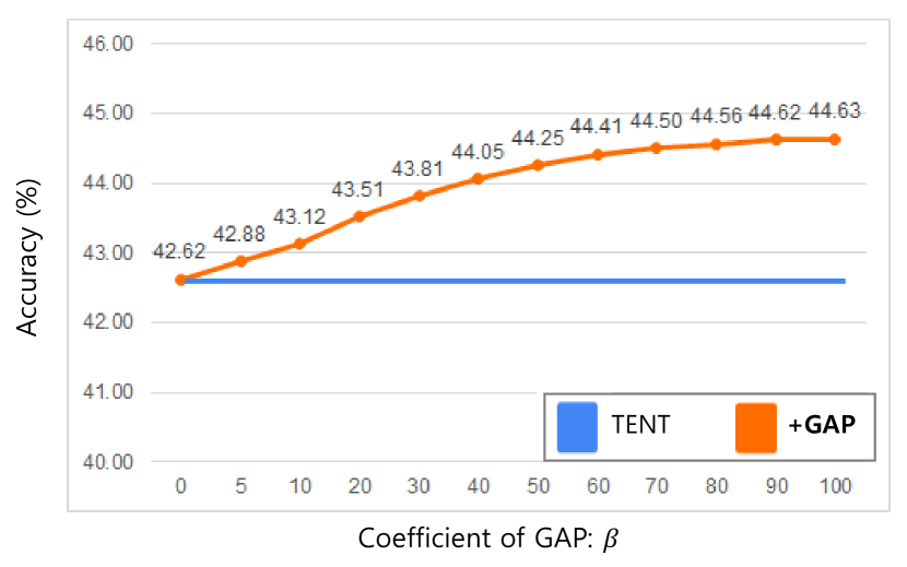
Figure 3: Sensitivity of the Average Classification Accuracy on ImageNet-C with respect tothe hyper-parameter $\beta$

$\gamma$	0	10	50	100	150	200
$Acc(\%)$	42.70	43.00	43.80	44.25	44.40	44.42

Table 8: Sensitivity of the Average classification Accuracy on ImageNet-C with respect tothe hyper-parameter $\gamma$

Figure 3 depicts the variation in the performance of the ImageNet-C dataset as the hyper-parameter $\beta$ changes. The plot illustrates the impact of incorporating the GAP regularizer compared to its absence and highlights sustained robust performance beyond a certain threshold. Table 8 presents the performance of the ImageNet-C dataset with respect to the variation in the hyper-parameter $\gamma$, which determines the decay rate. We chose $\gamma=100$, and it is observed that the performance remains nearly unchanged beyond 100.

5 Conclusion

In this study, we present a new approach called Gradient Alignment with Prototype feature (GAP) to improve the performance of test-time adaptation (TTA) scenarios. Our goal is to fine-tune the model for test data while maintaining high prediction accuracy for other data within the same class, ensuring robust generalization to unseen data. To achieve this, we introduce a prototype feature, aiming to maximize the reduction in loss associated with this feature. We employ the first-order Taylor expansion, expanding the equation and obtaining the dot product between the gradients of test data and prototype features. Next, we reformulate the GAP regularizer to make it computationally feasible for TTA situations. We approximate the prototype feature using the classifier’s weights and compute the gradient only for the weights corresponding to pseudo-labels while keeping the classifier fixed. This efficient computation allows us to calculate the GAP regularizer effectively. Our GAP regularizer is versatile and can be applied to any loss function where the gradient of the last layer can be efficiently computed. Furthermore, it can be combined with various existing methods. Experimental results demonstrate the effectiveness and robustness of the GAP regularizer across different benchmarks. In conclusion, our approach enhances model adaptability in TTA scenarios while maintaining broad applicability to diverse loss functions and methods.

References

- Anonymous [2024] Anonymous. Entropy is not enough for test-time adaptation: From the perspective of disentangled factors. In The Twelfth International Conference on Learning Representations, 2024.
- Arazo et al. [2020] Eric Arazo, Diego Ortego, Paul Albert, Noel E O’Connor, and Kevin McGuinness. Pseudo-labeling and confirmation bias in deep semi-supervised learning. In 2020 International Joint Conference on Neural Networks (IJCNN), pages 1–8. IEEE, 2020.
- Ashukha et al. [2020] Arsenii Ashukha, Alexander Lyzhov, Dmitry Molchanov, and Dmitry Vetrov. Pitfalls of in-domain uncertainty estimation and ensembling in deep learning. arXiv preprint arXiv:2002.06470, 2020.
- Bashkirova et al. [2022] Dina Bashkirova, Dan Hendrycks, Donghyun Kim, Haojin Liao, Samarth Mishra, Chandramouli Rajagopalan, Kate Saenko, Kuniaki Saito, Burhan Ul Tayyab, Piotr Teterwak, et al. Visda-2021 competition: Universal domain adaptation to improve performance on out-of-distribution data. In NeurIPS 2021 Competitions and Demonstrations Track, pages 66–79. PMLR, 2022.
- Croce et al. [2020] Francesco Croce, Maksym Andriushchenko, Vikash Sehwag, Edoardo Debenedetti, Nicolas Flammarion, Mung Chiang, Prateek Mittal, and Matthias Hein. Robustbench: a standardized adversarial robustness benchmark. arXiv preprint arXiv:2010.09670, 2020.
- Csurka [2017] Gabriela Csurka. Domain adaptation for visual applications: A comprehensive survey. arXiv preprint arXiv:1702.05374, 2017.
- Deng [2012] Li Deng. The mnist database of handwritten digit images for machine learning research [best of the web]. IEEE signal processing magazine, 29(6):141–142, 2012.
- Ganin and Lempitsky [2015] Yaroslav Ganin and Victor Lempitsky. Unsupervised domain adaptation by backpropagation. In International conference on machine learning, pages 1180–1189. PMLR, 2015.
- Gao et al. [2021] Zhiqiang Gao, Shufei Zhang, Kaizhu Huang, Qiufeng Wang, and Chaoliang Zhong. Gradient distribution alignment certificates better adversarial domain adaptation. In Proceedings of the IEEE/CVF International Conference on Computer Vision, pages 8937–8946, 2021.
- Goyal et al. [2022] Sachin Goyal, Mingjie Sun, Aditi Raghunathan, and Zico Kolter. Test-time adaptation via conjugate pseudo-labels. arXiv preprint arXiv:2207.09640, 2022.
- He et al. [2016] Kaiming He, Xiangyu Zhang, Shaoqing Ren, and Jian Sun. Deep residual learning for image recognition. In Proceedings of the IEEE conference on computer vision and pattern recognition, pages 770–778, 2016.
- Hendrycks and Dietterich [2019] Dan Hendrycks and Thomas Dietterich. Benchmarking neural network robustness to common corruptions and perturbations. arXiv preprint arXiv:1903.12261, 2019.
- Hendrycks et al. [2021] Dan Hendrycks, Steven Basart, Norman Mu, Saurav Kadavath, Frank Wang, Evan Dorundo, Rahul Desai, Tyler Zhu, Samyak Parajuli, Mike Guo, et al. The many faces of robustness: A critical analysis of out-of-distribution generalization. In Proceedings of the IEEE/CVF International Conference on Computer Vision, pages 8340–8349, 2021.
- Kar et al. [2022] Oğuzhan Fatih Kar, Teresa Yeo, Andrei Atanov, and Amir Zamir. 3d common corruptions and data augmentation. In Proceedings of the IEEE/CVF Conference on Computer Vision and Pattern Recognition, pages 18963–18974, 2022.
- Krizhevsky et al. [2017] Alex Krizhevsky, Ilya Sutskever, and Geoffrey E Hinton. Imagenet classification with deep convolutional neural networks. Communications of the ACM, 60(6):84–90, 2017.
- Lee and others [2013] Dong-Hyun Lee et al. Pseudo-label: The simple and efficient semi-supervised learning method for deep neural networks. In Workshop on challenges in representation learning, ICML, volume 3, page 896, 2013.
- Lee et al. [2022] Jonghyun Lee, Dahuin Jung, Junho Yim, and Sungroh Yoon. Confidence score for source-free unsupervised domain adaptation. In International Conference on Machine Learning, pages 12365–12377. PMLR, 2022.
- Liang et al. [2020] Jian Liang, Dapeng Hu, and Jiashi Feng. Do we really need to access the source data? source hypothesis transfer for unsupervised domain adaptation. In International Conference on Machine Learning, pages 6028–6039. PMLR, 2020.
- Mirza et al. [2022] M Jehanzeb Mirza, Jakub Micorek, Horst Possegger, and Horst Bischof. The norm must go on: dynamic unsupervised domain adaptation by normalization. In Proceedings of the IEEE/CVF Conference on Computer Vision and Pattern Recognition, pages 14765–14775, 2022.
- Mu and Gilmer [2019] Norman Mu and Justin Gilmer. Mnist-c: A robustness benchmark for computer vision. arXiv preprint arXiv:1906.02337, 2019.
- Muandet et al. [2013] Krikamol Muandet, David Balduzzi, and Bernhard Schölkopf. Domain generalization via invariant feature representation. In International conference on machine learning, pages 10–18. PMLR, 2013.
- Niu et al. [2022] Shuaicheng Niu, Jiaxiang Wu, Yifan Zhang, Yaofo Chen, Shijian Zheng, Peilin Zhao, and Mingkui Tan. Efficient test-time model adaptation without forgetting. In International conference on machine learning, pages 16888–16905. PMLR, 2022.
- Niu et al. [2023] Shuaicheng Niu, Jiaxiang Wu, Yifan Zhang, Zhiquan Wen, Yaofo Chen, Peilin Zhao, and Mingkui Tan. Towards stable test-time adaptation in dynamic wild world. arXiv preprint arXiv:2302.12400, 2023.
- Russakovsky et al. [2015] Olga Russakovsky, Jia Deng, Hao Su, Jonathan Krause, Sanjeev Satheesh, Sean Ma, Zhiheng Huang, Andrej Karpathy, Aditya Khosla, Michael Bernstein, et al. Imagenet large scale visual recognition challenge. International journal of computer vision, 115:211–252, 2015.
- Schneider et al. [2020] Steffen Schneider, Evgenia Rusak, Luisa Eck, Oliver Bringmann, Wieland Brendel, and Matthias Bethge. Improving robustness against common corruptions by covariate shift adaptation. Advances in Neural Information Processing Systems, 33:11539–11551, 2020.
- Shi et al. [2021] Yuge Shi, Jeffrey Seely, Philip HS Torr, N Siddharth, Awni Hannun, Nicolas Usunier, and Gabriel Synnaeve. Gradient matching for domain generalization. arXiv preprint arXiv:2104.09937, 2021.
- Snell et al. [2017] Jake Snell, Kevin Swersky, and Richard Zemel. Prototypical networks for few-shot learning. Advances in neural information processing systems, 30, 2017.
- Sun et al. [2020] Yu Sun, Xiaolong Wang, Zhuang Liu, John Miller, Alexei Efros, and Moritz Hardt. Test-time training with self-supervision for generalization under distribution shifts. In International conference on machine learning, pages 9229–9248. PMLR, 2020.
- Wang et al. [2021] Dequan Wang, Evan Shelhamer, Shaoteng Liu, Bruno Olshausen, and Trevor Darrell. Tent: Fully test-time adaptation by entropy minimization. In International Conference on Learning Representations, 2021.
- Zagoruyko and Komodakis [2016] Sergey Zagoruyko and Nikos Komodakis. Wide residual networks. arXiv preprint arXiv:1605.07146, 2016.
- Zeng et al. [2022] Ling-Li Zeng, Zhipeng Fan, Jianpo Su, Min Gan, Limin Peng, Hui Shen, and Dewen Hu. Gradient matching federated domain adaptation for brain image classification. IEEE Transactions on Neural Networks and Learning Systems, 2022.
- Zhang et al. [2022] Marvin Zhang, Sergey Levine, and Chelsea Finn. Memo: Test time robustness via adaptation and augmentation. Advances in Neural Information Processing Systems, 35:38629–38642, 2022.