Chiral Interaction Induced Near-Perfect Photon Blockade

Abstract

Based on the scattering matrix method, we theoretically demonstrate that the chiral interaction can induce the almost perfect photon blockade (PB) in the waveguide-cavity quantum electrodynamics (QED) system. The mechanism relies on the multi-photon-paths interference within the waveguide, which is clearly shown by the analytical parameter regime for $g^{(2)}(0)\approx 0$. When $N$ cavities are introduced into the system, there are $N$ optimal parameter points accordingly for the almost perfect PB, and the required chirality decreases exponentially with increasing $N$. Under the conditions of resonant driving and specific chirality, the output light only relies on the parity of $N$ ($N\geq 2$), where the coherent state and single-photon state correspond to the case of system including the odd and even number of cavities, respectively. Our work offers an alternative route for achieving almost perfect PB effects by employing the chirality of system, with potential application in the on-chip single-photon source with integrability.

Photon blockade [1], i.e., blockade of the subsequent photons by absorbing the first one [2, 3, 4], has attracted many significant theoretical and experimental attention in recent years, since its fundamental interest in exploring the quantum behavior of light [5, 6, 7] and potential applications in quantum information processing [8, 9, 10]. Considering the underlying physical mechanisms, PB effects generally can be categorized into conventional [1] and unconventional PBs [11, 12]. The conventional PB effect is induced by the anharmonicity in the spectrum of physical systems, and thus requires strong optical nonlinearities. This regime might be achieved in various systems, such as cavity QED systems [13, 14, 15, 16, 17], superconducting circuits [18, 19, 20], optomechanical resonators [21, 22, 23, 24], and so on [25, 26]. While the unconventional PB effect is caused by the interference effect among different transition paths within physical systems, and it can be achieved even in the weakly nonlinear regime.

With the rapid development of quantum computing, quantum simulation, and other emerging quantum technologies [27, 28, 29, 30, 31], the near-perfect PB effect, i.e., $g^{(2)}(0)\approx 0$, becomes increasingly significant for a large number of precision quantum devices, such as high-precision quantum gates [32, 33, 34], high-efficient single-photon devices [35, 36, 37], and other quantum devices [38, 39, 40, 41, 42, 43]. The waveguide QED systems offer an important platform for achieving the above precision quantum devices due to its unique design and operating principles, such as easy integration [44, 45], tunability, and high efficiency [46]. In particular, it is possible to achieve an interesting chiral interaction [47, 48] between the waveguide and cavity, i.e., the emission or scattering of photons from the cavity relies strongly on the photon’s propagation direction in a one-dimensional waveguide. Here the directionality originates from the interaction of elliptical dipoles with finely structured light fields of nanophotonic systems [49], such as nanowaveguides [50, 51], resonators [52, 53], and photonic-crystal (PhC) waveguides [54, 55, 48]. It has been demonstrated that the chiral interactions can induce interesting and important quantum effects, such as the directionality of spontaneous emission [48, 56] and chiral Purcell [57]. A natural question is whether it could influence the statistical properties of outgoing light significantly, and ultimately lead to the almost perfect PB effect.

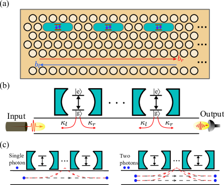
Figure 1: (a) The implementation of coupled waveguide-cavity QED system with PhC structure, including multiple point-defect H1-type PhC cavities coupled to semiconductor quantum dots, and a line-defect waveguide. (b) The general model of coupled waveguide-cavity QED system. Each cavity can emit photons to the left and right propagating waveguide modes, i.e., $b_{l}$ and $b_{r}$. The chirality of the cavity-waveguide interaction means the asymmetry of the corresponding decay rates $\kappa_{l}\neq\kappa_{r}$. (c) Illustrations of the single- and two-photon scattering processes in a waveguide.

Here we propose how to utilize the chiral interactions to achieve an almost perfect PB effect in a coupled waveguide-cavity QED system, which is experimentally feasible [58]. Based on the scattering matrix method, we provide a general analytical expression for the $n$th-order correlation functions with zero-time delay, and demonstrate the chiral interaction induced multi-photon-paths interference within waveguide. This interference effect can induce the near-perfect single-photon blockade (1PB), two-photon blockade (2PB), and photon-induced tunneling (PIT) by modulating the chiral waveguide-cavity interaction. In the case of system including $N$ cavities, we find that there are $N$ optimal parameter points for the almost perfect PB due to the increased interference paths. The chirality required for near-perfect PB decreases exponentially as the number of cavities $N$ increases. We also find and prove that, under the resonance driving condition, the almost perfect PB appears and disappears in the case of system including the odd and even number of cavities, respectively. Our work opens up a door for exploring the crossover between chiral quantum optics and the quantum state engineering, and offers potential applications in designing new types of high-purified single-photon devices.

Model and Hamiltonian.—As shown in Fig. 1(a), the system consists of multiple PhC cavities, and each cavity (denoted by annihilation operator $a_{j}$) is coupled to a two-level atom (denoted by lowering operator $\sigma_{j}\equiv|g\rangle_{j}\langle e|$) with the coupling strength g. Meanwhile, these cavities both are chirally side-coupled to a PhC waveguide, and the waveguide mode is described by a frequency-dependent annihilation operator $b_{\mu}(\omega)$, where $\mu=l$ and $r$ represent the left and right propagating modes, respectively. The annihilation operators satisfy a commutation relation $[b_{\mu}(\omega),b_{\mu^{\prime}}^{\dagger}(\omega^{\prime})]=\delta_{\mu,\mu^{\prime}}\delta(\omega-\omega^{\prime})$, and the interaction between the cavities and the waveguide is characterized by the decay rate $\kappa_{\mu}$. Here we find that the small decay rates of the atom does not essentially affect our results [59]. Therefore, we neglect the atom decay rates for simplicity since the decay rate of the cavity is much larger than that of the atom decay rates. Then, the total Hamiltonian of the coupled cavity-waveguide system is ($\hbar=1$) [60]

$$H_{\text{tot}}=H_{\text{sys}}+H_{\text{wg}}+H_{\text{int}}$$ (1)

with

$$H_{\text{sys}} =\sum_{j=1}^{N}[\omega_{c}a_{j}^{\dagger}a_{j}+\omega_{e}\sigma_{j}^{\dagger}\sigma_{j}+\text{g}(a_{j}^{\dagger}\sigma_{j}+\sigma_{j}^{\dagger}a_{j})],$$

$$H_{\text{wg}} =\sum_{\mu=l,r}{\int\differential\omega\ \omega b^{\dagger}_{\mu}(\omega)b_{\mu}(\omega)},$$ (2)

$$H_{\text{int}} =\sum_{j=1}^{N}\sum_{\mu=l,r}\sqrt{\frac{\kappa_{\mu}}{2\pi}}\int\differential\omega[b_{\mu}^{\dagger}(\omega)a_{j}e^{-i\omega x_{j}/v_{\mu}}+\text{h.c.}],$$

where $\omega_{c}$ is the cavity resonance frequency, $\omega_{e}$ is the transition frequency of atom, $\kappa_{l}$ and $\kappa_{r}$ are the decay rates into the left ($v_{l}<0$) and right ($v_{r}>0$) propagating waveguide modes, respectively. Moreover, $v_{\mu}$ denotes the corresponding group velocities in the waveguide (assuming $\absolutevalue{v_{r}}=\absolutevalue{v_{l}}=v$), and $x_{j}$ denotes the position of $j^{\text{th}}$ cavity. Without loss of generality, we assume the spacing of neighboring cavities is constant $d$ in the waveguide, and the atomic resonant frequency is the same as the cavity mode frequency, i.e., $\omega_{c}=\omega_{e}$. The chirality is defined as $\alpha\equiv\kappa_{l}/\kappa_{r}$ ($\alpha\in[0,1]$), with the perfectly chiral and nonchiral cases corresponding to $\alpha=0$ and $\alpha=1$, respectively.

Based on the scattering theory, we regard the cavity QED system as a potential field (or scatterer) [61] influencing the incident photons propagation within the waveguide, and the statistical properties of the output state could be completely described by the scattering processes of photons. As shown in Fig. 1(c), when a single photon is incident along the waveguide, there are two possible paths that the photon is scattered into the right-side output port. One is the free propagation along the waveguide shown by the black dotted line. The other is that the photon first is absorbed by the cavity QED system and then emitted into the right-side output port (i.e., right-moving mode), shown by the red dotted line. Similarly, for the incident of two photons without interaction, there are four possible paths: two photons are scattered into the right-side output port, and the photon-photon interactions can be induced by the presence of a potential field, as shown in the two red-dotted lines. Meanwhile, the two black-dotted lines represent the free propagating path without the influence of the potential field, and it cannot bring photon-photon interactions. The scattering matrix methods [62, 63, 64, 65, 66, 67, 68, 69, 70, 71, 72, 73, 74] are the optimal option to describe the scattering processes, and we only need to discuss few-photon scattering processes for our purpose. For the sake of simplicity, we consider the incident single-photon and two-photon with the frequencies $\omega_{d}$, and therefore the output states are given by [59]

$$|\Psi_{\text{out}}^{(1)}\rangle^{r} =\int\differential pS^{rr}_{p;\omega_{d}}b^{\dagger}_{r}(p)\ket{0},$$

$$|\Psi_{\text{out}}^{(2)}\rangle^{r} =\int\frac{\differential p_{1}\differential p_{2}}{2!\sqrt{2!}}S^{rr}_{p_{1}p_{2};\omega_{d}\omega_{d}}b^{\dagger}_{r}(p_{1})b^{\dagger}_{r}(p_{2})\ket{0},$$ (3)

where $S_{p;\omega_{d}}^{rr},S_{p_{1}p_{2};\omega_{d}\omega_{d}}^{rr}$ are the single- and two-photon scattering matrix elements, respectively. Here the superscripts $rr$ represent the input and output channels, respectively, which actually both are the right-moving waveguide mode. Notably, the scattering matrix elements completely can be characterized by the effective Hamiltonian [59]

$$H_{\text{eff}}\!=\!H_{\text{sys}} \!-\!i\sum_{j=1}^{N}\frac{\kappa}{2}a_{j}^{\dagger}a_{j}\!-\!i\sum_{j>k}^{N}e^{i\phi(j-k)}[\kappa_{r}a_{j}^{\dagger}a_{k}+\kappa_{l}a_{k}^{\dagger}a_{j}],$$ (4)

where $\kappa=\kappa_{l}+\kappa_{r}$ and $\phi=\omega_{c}d/v$. From now on, we only consider the case of mirror configuration ($\phi=2m\pi$ with $m\in\mathbb{N}$), which leads to $e^{i\phi(j-k)}=1$. For the other cases, it is analyzed in the Supplemental Materials [59].

Analytical nth-order correlation functions.—We consider a weak coherent state with amplitude $\beta$ entering into the waveguide from the left side channel, as shown in Fig. 1(b). The initial state of the total system is then given by

$$|\psi_{\text{in}}\rangle=\mathcal{N}\sum_{n=0}^{\infty}\frac{\beta^{n}}{\sqrt{n!}}|\Psi^{(n)}_{\text{in}}\rangle^{r}_{\omega_{d}}|0\rangle_{l}|0\rangle_{s},$$ (5)

where $|\Psi^{(n)}_{\text{in}}\rangle^{r}_{\omega_{d}}=[b_{r}^{\dagger n}(\omega_{d})/\sqrt{n!}]|0\rangle_{r}$ denotes the Fock state of $n$ photons with frequency $\omega_{d}$ in the right-moving waveguide mode. Here $|0\rangle_{r}$ and $|0\rangle_{l}$ are photonic vacuum states in the right-moving and left-moving waveguide modes, respectively. Moreover, $|0\rangle_{s}$ is the zero excitations eigenstate of the effective Hamiltonian, i.e., $H_{\text{eff}}|0\rangle_{s}=0$, and $\mathcal{N}$ is a normalization factor relying on $\beta$. According to the scattering theory, the output state could be written as $|\psi_{\text{out}}\rangle=S|\psi_{\text{in}}\rangle$, where $S$ is the scattering operator. Under the condition of weak-driving approximation, we establish a common expression for the $n$th-order correlation functions with zero-time delay in the output channel [75]

$$g_{rr}^{(n)}(0)=\lim\limits_{\absolutevalue{\beta}\to 0}\frac{\langle\psi_{\text{out}}|b_{r}^{\dagger n}(t)b_{r}^{n}(t)|\psi_{\text{out}}\rangle}{\ \langle\psi_{\text{out}}|b^{\dagger}_{r}(t)b_{r}(t)|\psi_{\text{out}}\rangle^{n}}=\frac{|\mathcal{P}_{n}|^{2}}{\ \ |\mathcal{P}_{1}|^{2n}},$$ (6)

where $\mathcal{P}_{n}$ represents the total probability amplitude of probing $n$-photon with zero-time delay in the right-side of waveguide. Considering all the possible scattering paths of $n$ incident photons, the total probability amplitude is actually a linear combination of probability amplitude of each possible path, which is given by

$$\begin{aligned} \mathcal{P}_{n}&=(2\pi)^{-\frac{n}{2}}\sum_{m=0}^{n}{C_{n}^{m}P^{N}_{m}\mathcal{I}_{n-m}}.\end{aligned}$$ (7)

Here, $P_{m}^{N}$ ($P^{N}_{0}=1$) represents the probability amplitude that $m$ photons first are absorbed by the system including $N$ cavities and then emitted into the right-moving waveguide mode, and $C_{n}^{m}$ is the combination number formula, including all the above possible paths. Moreover, $\mathcal{I}_{n-m}=\exp[-i(n-m)\omega_{d}t]$ denotes the probability amplitude of $(n-m)$ photons free propagation along the waveguide. Meanwhile, the incoming $n$ photons have $2^{n}$ possible paths if we numbered each photon, i.e., $\sum_{m=0}^{n}C_{n}^{m}=2^{n}$, and here the number $2$ represents two kinds of scattering paths of each single-photon, as shown in Fig. 1(c). The superposition of probability amplitude between these different paths produces the unique interference effect in the waveguide QED system, which ultimately induces the near-perfect photon blockade.

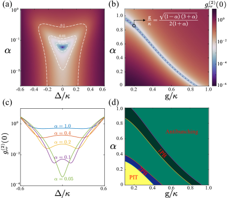
Figure 2: The equal-time second-order quantum correlation function $g_{rr}^{(2)}(0)$ versus the chirality $\alpha$ and (a) the detuning $\Delta/\kappa$, (b) the coupling strength $\text{g}/\kappa$. The white dotted lines in panel (a) represent the contour lines, corresponding to $g_{rr}^{(2)}(0)=0.1,\,0.01,\,0.001$. The dotted line in (b) indicates the parameter regime of $g_{rr}^{(2)}(0)=0$. (c) $g_{rr}^{(2)}(0)$ versus the detuning $\Delta/\kappa$ for different chirality. (d) Phase diagram illustrating the statistical properties of output photons. Here, the coupling strength $\text{g}/\kappa=0.8$ in (a, c), and the detuning $\Delta/\kappa=0$ in (b, d).

Near-perfect PB and phase diagram.—The above path interference in waveguide mainly depends on the chirality $\alpha=\kappa_{l}/\kappa_{r}$ of system and the number $N$ of cavities. We first consider the effect of chirality on PB in a single-cavity case ($N=1$). To obtain the second- and third-order quantum correlation function, we just need to compute $P^{N=1}_{n}$ with $n=1,2,3$ according to Eqs. (6-7). These probability amplitudes are given by

$$P^{N=1}_{1} =\frac{\xi_{\alpha}\Delta}{\Delta\Delta_{c}-\text{g}^{2}},P^{N=1}_{2}=\frac{\xi_{\alpha}^{2}(\text{g}^{2}+\Delta\Delta_{c}+\Delta^{2})}{\prod_{n=0}^{1}(n\Delta_{c}^{2}+\Delta\Delta_{c}-\text{g}^{2})},$$

$$P^{N=1}_{3} =\frac{\xi_{\alpha}^{3}[\prod_{n=0}^{2}(n\Delta_{c}+\Delta)+(4\Delta_{c}+3\Delta)\text{g}^{2}]}{\prod_{n=0}^{2}(n\Delta_{c}^{2}+\Delta\Delta_{c}-\text{g}^{2})},$$ (8)

where $\Delta=\omega_{c}-\omega_{d}$, $\Delta_{c}=\Delta-i\kappa/2$, and $\xi_{\alpha}/\kappa=ie^{-i\omega_{d}t}/(1+\alpha)$. Figures 2(a) and 2(c) show that the second-order correlation function approaches to zero around $\Delta/\kappa=0$ as decreasing the value of $\alpha$, i.e., $g_{rr}^{(2)}(0)|_{\alpha=1}\approx 1$ and $g_{rr}^{(2)}(0)|_{\alpha=0.05}\approx 10^{-4}$. For the ideal case of perfect PB, $g_{rr}^{(2)}(0)=0$ corresponds to the probability of equal-time probing two-photon in the output channel is equal to zero, i.e., $\mathcal{P}_{2}=0$. Physically, only when the two-photon paths destructive interference happens, the second-order quantum correlation function will be zero. At the resonant condition, i.e., $\Delta=0$, the analytical parameters condition for perfect PB, i.e., $g_{rr}^{(2)}(0)=0$, is

$$\text{g}/\kappa=\frac{\sqrt{(1-\alpha)(3+\alpha)}}{2(1+\alpha)}\ (0\leq\alpha<1)$$ (9)

corresponding to the white dotted line in Fig. 2(b). Equation (9) clearly demonstrates that the perfect PB effect only happens in the situation of the system being chirality, i.e., $\alpha<1$, which induces the two-photon paths destructive interference. In addition, we also study some interesting quantum phenomena besides 1PB, such as 2PB and PIT. For the criterion of 2PB, the correlation functions have to fulfill $g_{rr}^{(3)}(0)<1$ and $g_{rr}^{(2)}(0)\geq 1$ [43]. The criterion for PIT is $g_{rr}^{(n)}(0)>1$ for $n=2,3$ [43]. Combining these criteria, we present the phase diagram describing the statistical properties of output photons in Fig. 2(d). Note that the criterion of 1PB corresponds to $g_{rr}^{(2)}(0)<0.01$ here. It is clearly shown that the 2PB and PIT only appear in the region with chirality. This phase diagram brings an intuitive understanding of the statistical properties of outgoing light in different parameter regions.

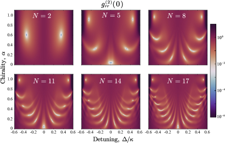
Figure 3: The equal-time second-order quantum correlation function $g_{rr}^{(2)}(0)$ versus the chirality $\alpha$ and the detuning $\Delta/\kappa$, for various sizes $N$. The parameters, for each $N$, are the same as in Fig. 2(a).

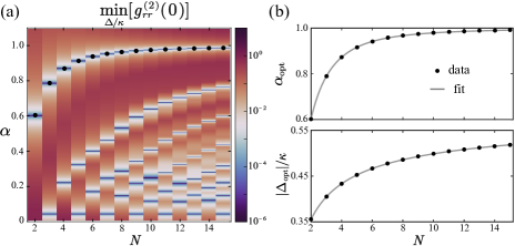
Figure 4: (a) The minimum second-order correlation function as a function of the chirality $\alpha$ and the number of cavities $N$. Dots indicate the lowest chirality $\alpha_{\text{opt}}$ leading to the near-perfect PB effect: $\alpha_{\text{opt}}$ tends to the nonchiral case for large $N$. (b) Top: optimal chirality $\alpha_{\text{opt}}$ as a function of $N$. Gray line is a fit with the function $f(N)=1-N^{\eta}\sum_{i=1}^{2}c_{i}\exp(-a_{i}N)$ for $N>1$ (main: $a_{1}=0.456,a_{2}=0.089,c_{1}=1.103,c_{2}=0.294,\eta=-0.795$). Bottom: the correspondingly optimal detuning $|\Delta_{\text{opt}}|/\kappa$ as a function of $N$. Gray line is a fit with the function $h(N)=0.593-c_{3}N^{\gamma}$ for $N>1$ (main: $c_{3}=0.534,\gamma=-0.574$). The other parameters are the same as in Fig. 2(a).

The case of multi-cavity.—As the number of cavities increases, the possible interference paths of the incoming photons among different cavities will increase accordingly. This results in an increase of the number of antibunching points corresponding to $g_{rr}^{(2)}(0)\ll 1$. Figure 3 illustrates that the system exhibits $N$ near-perfect PB points, and a larger $N$ also leads to wider PB windows. These observations highlight the progressive enhancement of PB effects with the expansion of the cavity-atom array. Furthermore, our results reveal another intriguing phenomenon: under the resonant condition ($\Delta=0$), the near perfect PB effect completely disappears for systems with an even number of cavities [$N=2j$ with $j\in\mathbb{N}$], i.e., $g_{rr}^{(2)}(0)=1$. However, it remarkably reappears for systems with an odd number of cavities [$N=2j+1$ with $j\in\mathbb{N}$]. To elucidate this intriguing phenomenon, we begin by investigating the case of single-photon scattering processes. Referring to Eq. (8), we have $P^{N=1}_{1}=0$ at the resonant condition, which also holds for multiple cavities, i.e., $P_{1}^{N}=0$. Subsequently, for multi-photon scattering processes, we regard the two adjacent-cavity systems as a single unit cell to simplify the calculation. For each cell, we find that the $n$-photon scattering matrix is characterized by $S^{rr}_{p_{1}\ldots p_{n};\omega_{c}\ldots\omega_{c}}=n!\prod_{j=1}^{n}\delta(p_{j}-\omega_{c})$, which implies $P_{n}^{N=2}=0$. As a result, we can obtain $P_{n}^{N=2j}=0$ with $j\in\mathbb{N}$ [59], and the output light naturally retains the statistical properties of input state for systems with the even number of cavities, i.e., $|\psi_{\text{out}}\rangle=|\psi_{\text{in}}\rangle$. However, in the case of the odd number of cavities, although the scattering processes of two photons align with the previously discussed behavior for the first $2j$ cavities, there exits multi-photon path interference between the first $2j$ cavities and the last cavity, which leads to [59]

$$P_{2}^{N=2j+1}=\frac{-4e^{-2i\omega_{c}t}(1-\alpha)^{2}/(1+\alpha^{2})}{\left[4(\text{g}/\kappa)^{2}(1+\alpha)^{2}+(1-\alpha)^{2}\right]}.$$ (10)

Comparing with the case of the even number of cavities, Eq. (10) clearly show that the near-perfect PB reemerges when the system is in the appropriate chirality. Note that, the scattering matrix method used in this main text agrees perfectly with the matrix product states simulations [59].

To extract more information regarding the PB property, we iterate over all the detuning values for the fixed chirality and $N$ to obtain the minimum second-order correlation function $\min\limits_{\Delta/\kappa}[g_{rr}^{(2)}(0)]$ in Fig. 4(a). Each dark-blue transverse fringe corresponds to a near-perfect PB point, and interestingly, the number of fringes equals $\lceil N/2\rceil$ for any given $N$. More importantly, Fig. 4(b) shows that the lowest chirality required for achieving near perfect PB exhibits an exponential decrease with the number of cavities $N$, i.e., $1-\alpha_{\text{opt}}\propto\exp(-a_{i}N)\text{ with }a_{i}>0$. Additionally, the corresponding detuning also obeys power law relationship, i.e., $0.593-\absolutevalue{\Delta_{\text{opt}}}/\kappa\propto N^{\gamma}\text{ with }\gamma<0$. These intriguing findings stem from the exponential growth of interference paths between different cavities, resulting in the emergence of PB even in systems with weak chirality. This property opens the door to significantly reducing the required chirality rate for obtaining a high purified single-photon source.

Conclusion.—In conclusion, we have demonstrated a condition inducing near-perfect PB when the cavity couples asymmetrically to the left and right propagating modes of the waveguide. We have provided analytically the optimal parameter region in the case of a single cavity based on the scattering matrix method. Moreover, we also numerically showed that the required chirality for near-perfect PB decreases exponentially with the number of cavities. Our work can be used to realize scalable single-photon sources [76, 44] using a mature PhC waveguide platform, which might have a significant impact for quantum information science applications. It also can inspire the following studies of other quantum effects induced by a chiral couping of the cavities to the waveguide modes and provides a promising scheme to probe the underlying many-body states of the system.

This work is supported by the National Key Research and Development Program of China grant 2021YFA1400700 and the National Natural Science Foundation of China (Grant No. 11974125).

Supplemental Material for
“Chiral Interaction Induced Near-Perfect Photon Blockade”

Zhi-Guang Lu¹, Ying Wu¹, Xin-You Lü¹

¹School of Physics and Institute for Quantum Science and Engineering, Huazhong University of Science and Technology, Wuhan 430074, China

This supplement material contains five parts: I. A detailed derivation for the connection between the scattering matrix ($S$ matrix) and the effective Hamiltonian; II. A detailed discussion of the case of multi-cavity under the resonance condition; III. A detailed discussion about the effect of non-mirror configuration; IV. A detailed discussion about the effect of atomic dissipation. V. A detail about the matrix product states (MPS) simulations.

S1 Proof for the connection between the $S$ matrix and the effective Hamiltonian

In this section, we provide a detailed proof to support Eq. (4) in the main text, explaining the connection between the $S$ matrix elements and the effective Hamiltonian in the waveguide-cavity quantum electrodynamics (QED) system under the Markovian approximation.

S1.1 The input-output formalism and the quantum causality relation

Firstly, the total Hamiltonian describing multiple cavities coupling to a two-mode waveguide reads as

$$H_{\text{tot}}=H_{\text{sys}}+\sum_{\mu=l,r}\int\differential{\omega}\ \omega b_{\mu}^{\dagger}(\omega)b_{\mu}(\omega)+\sum_{j=1}^{N}\sum_{\mu=l,r}\sqrt{\frac{\kappa_{\mu}}{2\pi}}\int\differential{\omega}[b_{\mu}^{\dagger}(\omega)a_{j}e^{-i\omega x_{j}/v_{\mu}}+a^{\dagger}_{j}b_{\mu}(\omega)e^{i\omega x_{j}/v_{\mu}}],$$ (S1)

where $H_{\text{sys}}=\sum_{j=1}^{N}[\omega_{c}a_{j}^{\dagger}a_{j}+\omega_{e}\sigma_{j}^{\dagger}\sigma_{j}+\text{g}(a_{j}^{\dagger}\sigma_{j}+\sigma_{j}^{\dagger}a_{j})]$ and $x_{j}=(j-1)d$. Then, we select a rotating frame, and the corresponding unitary transformation is represented by $U_{0}=\exp(iH_{0}t)$, where

$$H_{0}=\omega_{d}\sum_{j=1}^{N}[a_{j}^{\dagger}a_{j}+\sigma^{\dagger}_{j}\sigma_{j}]+\omega_{d}\sum_{\mu=l,r}\int\differential{\omega}b_{\mu}^{\dagger}(\omega)b_{\mu}(\omega).$$ (S2)

Thus, the total Hamiltonian under the rotating frame can be written as

$$\tilde{H}_{\text{tot}}=U_{0}H_{\text{tot}}U_{0}^{\dagger}+i(\partial_{t}U_{0})U_{0}^{\dagger},$$ (S3)

and the Heisenberg equations of motion are

$$\frac{\differential}{\differential t}\tilde{b}_{\mu}(\omega) =-i(\omega-\omega_{d})\tilde{b}_{\mu}(\omega)-i\sum_{j=1}^{N}\sqrt{\frac{\kappa_{\mu}}{2\pi}}\tilde{a}_{j}e^{-i\omega x_{j}/v_{\mu}},$$ (S4a)

$$\frac{\differential}{\differential t}\tilde{a}_{m} =-i[\tilde{a}_{m},\tilde{H}_{\text{sys}}]-i\sum_{\mu=l,r}\sqrt{\frac{\kappa_{\mu}}{2\pi}}\int\differential{\omega}\tilde{b}_{\mu}(\omega)e^{i\omega x_{m}/v_{\mu}},$$ (S4b)

where $\tilde{H}_{\text{sys}}=\sum_{j=1}^{N}[(\omega_{c}-\omega_{d})\tilde{a}_{j}^{\dagger}\tilde{a}_{j}+(\omega_{e}-\omega_{d})\tilde{\sigma}_{j}^{\dagger}\tilde{\sigma}_{j}+\text{g}(\tilde{a}_{j}^{\dagger}\tilde{\sigma}_{j}+\tilde{\sigma}_{j}^{\dagger}\tilde{a}_{j})]$, and the tildes indicate operators after transformation $U_{0}$ (i.e., in the rotating frame). We then define the input and output operators as

$$\tilde{b}_{\mu,\text{in}}(t) \equiv\int\frac{\differential{\omega}}{\sqrt{2\pi}}\tilde{b}_{\mu}(\omega,t_{0})e^{-i(\omega-\omega_{d})(t-t_{0})},\quad t_{0}\to-\infty,$$ (S5a)

$$\tilde{b}_{\mu,\text{out}}(t) \equiv\int\frac{\differential{\omega}}{\sqrt{2\pi}}\tilde{b}_{\mu}(\omega,t_{1})e^{-i(\omega-\omega_{d})(t-t_{1})},\quad t_{1}\to+\infty.$$ (S5b)

After multiplying Eq. (S4a) by the integration factor $\exp[i(\omega-\omega_{d})t]$, we integrate it from an initial time $t_{0}<t$ to obtain

$$\tilde{b}_{\mu}(\omega,t)=\tilde{b}_{\mu}(\omega,t_{0})e^{-i(\omega-\omega_{d})(t-t_{0})}-i\sum_{j=1}^{N}\sqrt{\frac{\kappa_{\mu}}{2\pi}}\int_{t_{0}}^{t}\differential{t^{\prime}}\tilde{a}_{j}(t^{\prime})e^{-i(\omega-\omega_{d})(t+x_{j}/v_{\mu}-t^{\prime})}e^{-i\omega_{d}x_{j}/v_{\mu}}.$$ (S6)

Combining with Eq. (S5a), we integrate Eq. (S6) with respect to $\omega$ and obtain

$$\int\frac{\differential{\omega}}{\sqrt{2\pi}}\tilde{b}_{\mu}(\omega,t)=\tilde{b}_{\mu,\text{in}}(t)-i\sqrt{\kappa_{\mu}}\sum_{j=1}^{N}e^{-i\omega_{d}x_{j}/v_{\mu}}\int_{t_{0}}^{t}\differential{t^{\prime}}\tilde{a}_{j}(t^{\prime})\delta(t+x_{j}/v_{\mu}-t^{\prime}).$$ (S7)

Similarly, we integrate Eq. (S4a) up to a final time $t_{1}>t$, and take advantage of Eq. (S5b), which results in

$$\int\frac{\differential{\omega}}{\sqrt{2\pi}}\tilde{b}_{\mu}(\omega,t)=\tilde{b}_{\mu,\text{out}}(t)+i\sqrt{\kappa_{\mu}}\sum_{j=1}^{N}e^{-i\omega_{d}x_{j}/v_{\mu}}\int_{t}^{t_{1}}\differential{t^{\prime}}\tilde{a}_{j}(t^{\prime})\delta(t+x_{j}/v_{\mu}-t^{\prime}).$$ (S8)

Under the usual Markovian approximation, i.e., $\absolutevalue{\omega_{c}-\omega_{d}},\absolutevalue{\omega_{e}-\omega_{d}},\text{g},\kappa_{\mu}\ll\absolutevalue{v_{\mu}}/\max\limits_{j,l}\absolutevalue{x_{j}-x_{l}}$, we have $\tilde{a}_{j}(t\pm\absolutevalue{x_{j}/v_{\mu}})\approx\tilde{a}_{j}(t)$ and $\exp(-i\omega_{d}x_{j}/v_{\mu})\approx\exp(-i\omega_{c}x_{j}/v_{\mu})$. As a result, we could derive the following input-output formalism from the above Eqs. (S7,S8) and obtain

$$\tilde{b}_{\mu,\text{out}}(t)=\tilde{b}_{\mu,\text{in}}(t)-i\sqrt{\kappa_{\mu}}\sum_{j=1}^{N}e^{-i\omega_{c}x_{j}/v_{\mu}}\tilde{a}_{j}(t).$$ (S9)

Furthermore, substituting Eq. (S7) and Eq. (S8) into Eq. (S4b) results in

$$\frac{\differential}{\differential t}\tilde{a}_{m}(t)= -i[\tilde{a}_{m}(t),\tilde{H}_{\text{sys}}]-i\sum_{\mu=l,r}\sqrt{\frac{\kappa_{\mu}}{2\pi}}\tilde{b}_{\mu,\text{in}}(t)e^{i\omega_{d}x_{m}/v_{\mu}}-\frac{\kappa_{l}+\kappa_{r}}{2}\tilde{a}_{m}(t)$$

$$-\sum_{n=1}^{m-1}\kappa_{r}e^{-i\omega_{d}(x_{n}-x_{m})/v_{r}}\tilde{a}_{n}(t)-\sum_{n=m+1}^{N}\kappa_{l}e^{-i\omega_{d}(x_{n}-x_{m})/v_{l}}\tilde{a}_{n}(t),$$ (S10a)

$$\frac{\differential}{\differential t}\tilde{a}_{m}(t)= -i[\tilde{a}_{m}(t),\tilde{H}_{\text{sys}}]-i\sum_{\mu=l,r}\sqrt{\frac{\kappa_{\mu}}{2\pi}}\tilde{b}_{\mu,\text{out}}(t)e^{i\omega_{d}x_{m}/v_{\mu}}+\frac{\kappa_{l}+\kappa_{r}}{2}\tilde{a}_{m}(t)$$

$$+\sum_{n=1}^{m-1}\kappa_{r}e^{-i\omega_{d}(x_{n}-x_{m})/v_{r}}\tilde{a}_{n}(t)+\sum_{n=m+1}^{N}\kappa_{l}e^{-i\omega_{d}(x_{n}-x_{m})/v_{l}}\tilde{a}_{n}(t).$$ (S10b)

Based on Eqs. (S10a,S10b), we could obtain a crucial property, namely quantum causality relation, which states that

$$[\tilde{a}_{m}(t),\tilde{b}_{\mu,\text{in}}(t^{\prime})]=[\tilde{a}^{\dagger}_{m}(t),\tilde{b}_{\mu,\text{in}}(t^{\prime})]=[\tilde{a}_{m}(t),\tilde{b}^{\dagger}_{\mu,\text{in}}(t^{\prime})]=[\tilde{a}^{\dagger}_{m}(t),\tilde{b}^{\dagger}_{\mu,\text{in}}(t^{\prime})]=0,\text{for}\ t\leq t^{\prime},$$ (S11a)

$$[\tilde{a}_{m}(t),\tilde{b}_{\mu,\text{out}}(t^{\prime})]=[\tilde{a}^{\dagger}_{m}(t),\tilde{b}_{\mu,\text{out}}(t^{\prime})]=[\tilde{a}_{m}(t),\tilde{b}^{\dagger}_{\mu,\text{out}}(t^{\prime})]=[\tilde{a}^{\dagger}_{m}(t),\tilde{b}^{\dagger}_{\mu,\text{out}}(t^{\prime})]=0,\text{for}\ t\geq t^{\prime}.$$ (S11b)

S1.2 The $S$ matrix and the effective Hamiltonian

Here, we consider such a scattering process, i.e., incoming $n$ photons from the left-side input port being scattered into the right-side output port, and the process can be described by $n$-photon $S$ matrix elements. Combining with the definitions of input and output operators (S5a, S5b), the $n$-photon $S$ matrix elements can be written as

$$\tilde{S}_{p_{1}\ldots p_{n};k_{1}\ldots k_{n}}^{rr}=\left[\prod_{l=1}^{n}\frac{\differential{t_{l}^{\prime}}}{\sqrt{2\pi}}e^{i(p_{l}-\omega_{d})t_{l}^{\prime}}\prod_{j=1}^{n}\frac{\differential{t_{j}}}{\sqrt{2\pi}}e^{-i(k_{j}-\omega_{d})t_{j}}\right]\langle 0|\prod_{l=1}^{n}\tilde{b}_{r,\text{out}}(t^{\prime}_{l})\prod_{j=1}^{n}\tilde{b}^{\dagger}_{r,\text{in}}(t_{j})|0\rangle,$$ (S12)

and we need to compute the time-domain $n$-photon $S$ matrix,

$$\tilde{S}^{rr}_{t_{1}^{\prime}\ldots t_{n}^{\prime};t_{1}\ldots t_{n}}\equiv\langle 0|\prod_{l=1}^{n}\tilde{b}_{r,\text{out}}(t_{l}^{\prime})\prod_{j=1}^{n}\tilde{b}^{\dagger}_{r,\text{in}}(t_{j})|0\rangle.$$ (S13)

Here for simplicity, let us set $\tilde{A}_{\mu,\omega}(t)\equiv\sqrt{\kappa_{\mu}}\sum_{j=1}^{N}e^{-i\omega x_{j}/v_{\mu}}\tilde{a}_{j}(t)$, where $\mu\in\{l,r\}$. By utilizing the input-output relation Eq. (S9) and the quantum causality relation Eqs. (S11a,S11b), we can simplify the computation of the $S$ matrix. This simplification transforms the computation into that of the Green’s function, which solely consists of the operator $\tilde{A}_{r,\omega_{c}}$ [1]. Consequently, we focus on evaluating the time-ordered $2M$-point Green’s function

$$\tilde{G}^{rr}(t^{\prime}_{1},\ldots,t^{\prime}_{M};t_{1},\ldots,t_{M})\equiv(-1)^{M}\langle 0|\mathcal{T}[\tilde{A}_{r,\omega_{c}}(t_{1}^{\prime})\cdots\tilde{A}_{r,\omega_{c}}(t_{M}^{\prime})\tilde{A}^{\dagger}_{r,\omega_{c}}(t_{1})\cdots\tilde{A}^{\dagger}_{r,\omega_{c}}(t_{M})]|0\rangle,$$ (S14)

where $\mathcal{T}$ is a time-ordered symbol. In order to prove the Green’s functions can be computed by using the effective Hamiltonian, we start by the path integral formulation of the Green’s function, i.e.,

$$\tilde{G}^{rr}(t_{1}^{\prime},\ldots,t_{M}^{\prime};t_{1},\ldots,t_{M})=(-1)^{M}\frac{\int\mathcal{D}[\{\tilde{b}_{\mu}(\omega),\tilde{b}^{*}_{\mu}(\omega)\},\{\tilde{a}_{j},\tilde{a}^{*}_{j}\}]\prod_{j=1}^{M}\tilde{A}_{r,\omega_{c}}(t^{\prime}_{j})\prod_{l=1}^{M}\tilde{A}_{r,\omega_{c}}^{*}(t_{l})e^{i\int\differential{t}\tilde{\mathcal{L}}}}{\int\mathcal{D}[\{\tilde{b}_{\mu}(\omega),\tilde{b}^{*}_{\mu}(\omega)\},\{\tilde{a}_{j},\tilde{a}^{*}_{j}\}]e^{i\int\differential{t}\tilde{\mathcal{L}}}},$$ (S15)

where

$$\tilde{\mathcal{L}}=\sum_{\mu=l,r}\int\differential{\omega}\{\tilde{b}_{\mu}^{*}(\omega)[i\partial_{t}-(\omega-\omega_{d})]\tilde{b}_{\mu}(\omega)-[\tilde{b}_{\mu}^{*}(\omega)\tilde{A}_{\mu,\omega}(t)+\tilde{A}_{\mu,\omega}\tilde{b}_{\mu}(\omega)]/\sqrt{2\pi}\}+\tilde{\mathcal{L}}_{\text{sys}}$$ (S16)

is the Lagrangian associated with the total Hamiltonian (S3) and $\tilde{\mathcal{L}}_{\text{sys}}$ is the local system’s Lagrangian obtained by Legendre transformation on the system’s Hamiltonian $\tilde{H}_{\text{sys}}$. Meanwhile, we define a symbol $\mathcal{A}=\partial_{t}+i(\omega-\omega_{d})$ and introduce the propagator of the free waveguide photon

$$G_{\omega}^{(0)}(t-t^{\prime})\equiv\int\frac{\differential{k}}{2\pi}e^{-ik(t-t^{\prime})}\frac{i}{k-\omega+i0^{+}}=e^{-i\omega(t-t^{\prime})}\Theta(t-t^{\prime}),$$ (S17)

where $\Theta(t)$ is the step function. Notably, the propagator is the inverse of $\mathcal{A}$, i.e., $\mathcal{A}G_{\omega-\omega_{d}}^{(0)}(t-t^{\prime})=\delta(t-t^{\prime})$.

Finally, we integrate out the waveguide degrees of freedom

$$\int\mathcal{D}[\{\tilde{b}_{\mu}(\omega),\tilde{b}^{*}_{\mu}(\omega)\}]e^{i\int\differential{t}\tilde{\mathcal{L}}} =e^{i\int\differential{t}\tilde{\mathcal{L}}_{\text{sys}}}\int\mathcal{D}[\{\tilde{b}_{\mu}(\omega),\tilde{b}^{*}_{\mu}(\omega)\}]e^{-\sum_{\mu=l,r}\int\differential{t}\int\differential{\omega}[\tilde{b}_{\mu}^{*}(\omega)\mathcal{A}\tilde{b}_{\mu}(\omega)+i\frac{\tilde{b}_{\mu}^{*}(\omega)\tilde{A}_{\mu,\omega}(t)+\tilde{A}^{*}_{\mu,\omega}(t)\tilde{b}_{\mu}(\omega)}{\sqrt{2\pi}}]}$$

$$=\mathscr{N}e^{i\int\differential{t}\tilde{\mathcal{L}}_{\text{sys}}-\sum_{\mu=l,r}\int\differential{t}\int\differential{t^{\prime}}\int\differential{\omega}\tilde{A}_{\mu,\omega}(t)G_{\omega-\omega_{d}}^{(0)}(t-t^{\prime})\tilde{A}_{\mu,\omega}(t^{\prime})/(2\pi)}$$

$$=\mathscr{N}e^{i\int\differential{t}\tilde{\mathcal{L}}_{\text{sys}}-\sum_{\mu=l,r}\int\differential{t}\int\differential{t^{\prime}}\kappa_{\mu}\sum_{j,k=1}^{N}\tilde{a}_{j}^{*}(t)\tilde{a}_{k}(t^{\prime})e^{i\omega_{d}(x_{j}-x_{k})/v_{\mu}}\delta(t-t^{\prime}-\frac{x_{j}-x_{k}}{v_{\mu}})\Theta(t-t^{\prime})}$$

$$=\mathscr{N}e^{i\int\differential{t}\tilde{\mathcal{L}}_{\text{sys}}-\int\differential{t}\sum_{\mu=l,r}\kappa_{\mu}\sum_{j,k=1}^{N}\tilde{a}_{j}^{*}(t)\tilde{a}_{k}(t)e^{-i\omega_{c}(x_{k}-x_{j})/v_{\mu}}\Theta(\frac{x_{j}-x_{k}}{v_{\mu}})}$$

$$=\mathscr{N}e^{i\int\differential{t}\tilde{\mathcal{L}}_{\text{eff}}},$$ (S18)

where $\mathscr{N}$ is the constant coefficient from the Gaussian functional integration. In the fourth step, we use the Markovian approximation. In the last step, the effective Lagrangian can be written as

$$\tilde{\mathcal{L}}_{\text{eff}}=\tilde{\mathcal{L}}_{\text{sys}}+i\sum_{j=1}^{N}\frac{\kappa_{l}+\kappa_{r}}{2}\tilde{a}_{j}^{*}\tilde{a}_{j}+i\sum_{j>k}^{N}e^{i\omega_{c}(x_{j}-x_{k})/v_{r}}[\kappa_{r}\tilde{a}_{j}^{*}\tilde{a}_{k}+\kappa_{l}\tilde{a}_{k}^{*}\tilde{a}_{j}],$$ (S19)

and the corresponding effective Hamiltonian is obtained from the effective Lagrangian by Legendre transformation, i.e.,

$$\tilde{H}_{\text{eff}}=\tilde{H}_{\text{sys}}-i\sum_{j=1}^{N}\frac{\kappa_{l}+\kappa_{r}}{2}\tilde{a}_{j}^{\dagger}\tilde{a}_{j}-i\sum_{j>k}^{N}e^{i\omega_{c}(x_{j}-x_{k})/v_{r}}[\kappa_{r}\tilde{a}_{j}^{\dagger}\tilde{a}_{k}+\kappa_{l}\tilde{a}_{k}^{\dagger}\tilde{a}_{j}].$$ (S20)

As a result, Eq. (S15) is simplified further as

$$\tilde{G}^{rr}(t_{1}^{\prime},\ldots,t_{M}^{\prime};t_{1},\ldots,t_{M}) =(-1)^{M}\frac{\int\mathcal{D}[\{\tilde{a}_{j},\tilde{a}^{*}_{j}\}]\prod_{j=1}^{M}\tilde{A}_{r,\omega_{c}}(t^{\prime}_{j})\prod_{l=1}^{M}\tilde{A}_{r,\omega_{c}}^{*}(t_{l})e^{i\int\differential{t}\tilde{\mathcal{L}}_{\text{eff}}}}{\int\mathcal{D}[\{\tilde{a}_{j},\tilde{a}^{*}_{j}\}]e^{i\int\differential{t}\tilde{\mathcal{L}}_{\text{eff}}}}$$

$$={G}^{rr}(t_{1}^{\prime},\ldots,t_{M}^{\prime};t_{1},\ldots,t_{M})\equiv(-1)^{M}\langle 0|\mathcal{T}[\prod_{j=1}^{M}{A}_{r,\omega_{c}}(t_{j}^{\prime})\prod_{l=1}^{M}{A}^{\dagger}_{r,\omega_{c}}(t_{l})]|0\rangle,$$ (S21)

with operators

$${A}_{r,\omega_{c}}(t)=e^{iH_{\text{eff}}t}A_{r,\omega_{c}}e^{-iH_{\text{eff}}t},\quad{A}^{\dagger}_{r,\omega_{c}}(t)=e^{iH_{\text{eff}}t}A^{\dagger}_{r,\omega_{c}}e^{-iH_{\text{eff}}t},$$ (S22)

where

$$H_{\text{eff}}=H_{\text{sys}}-i\sum_{j=1}^{N}\frac{\kappa_{r}+\kappa_{l}}{2}a_{j}^{\dagger}a_{j}-i\sum_{j>k}^{N}e^{i\phi(j-k)}[\kappa_{r}a_{j}^{\dagger}a_{k}+\kappa_{l}a_{k}^{\dagger}a_{j}],$$ (S23)

with $\phi=\omega_{c}d/v_{r}$. In the second and last steps of Eq. (S1.2), we have already reverted to the original frame [i.e., Eq. (S1)] and removed the tildes so as to indicate system’s operators after the corresponding transformation. Accordingly, the $S$ matrix elements should also take off the coefficient $\omega_{d}$ in Eq. (S12) when the whole system reverts to the original frame. Thus, we have obtained the effective Hamiltonian Eq. (4) in the main text, as shown in Eq. (S23), and proved that the computation of the scattering matrix elements are completely depended on the effective Hamiltonian for the system without involving the waveguide photon’s degree of freedom.

S2 Discussion of the case of multi-cavity under the resonance condition

To support Eq. (3) and the case of multi-cavity under the resonance condition in the main text, in this section, we provide the detailed derivation for the multi-photon $S$ matrix elements and the second-order equal-time correlation function. For this purpose, we again introduce the scattering process mentioned at Sec. S1.2 and assume that the frequencies of incoming $n$ photons are all $\omega_{d}$. Therefore, the input state can be defined as $|\Psi_{\text{in}}^{(n)}\rangle^{r}_{\omega_{d}}=[b^{\dagger n}_{r}(\omega_{d})/\sqrt{n!}]|0\rangle_{r}$, and the output state being scattered into the right-side waveguide is given by

$$|\Psi_{\text{out}}^{(n)}\rangle^{r}=\int\frac{\prod_{j=1}^{n}\differential{p_{j}}}{n!\sqrt{n!}}[\prod_{j=1}^{n}b^{\dagger}_{r}(p_{j})]|0\rangle\langle 0|[\prod_{j=1}^{n}b_{r}(p_{j})]{S}[b_{r}^{\dagger n}(\omega_{d})]|0\rangle_{r}=\int\frac{\prod_{j=1}^{n}\differential{p_{j}}}{n!\sqrt{n!}}{S}^{rr}_{p_{1}\ldots p_{n};\omega_{d}\ldots\omega_{d}}[\prod_{j=1}^{n}b^{\dagger}_{r}(p_{j})]|0\rangle_{r}.$$ (S24)

When we consider the cases of $n=1$ and $n=2$, Eq. (S24) will give Eq. (3) of the main text. Besides, for the single-photon $S$ matrix, we have

$${S}_{p;\omega_{d}}^{rr}=\delta(p-\omega_{d})[1+O_{0,1}\mathcal{K}^{-1}_{\omega_{d}}(1)O_{0,1}^{\dagger}],$$ (S25)

where $\mathcal{K}_{\omega}(n)=-i[H_{\text{eff}}^{(n)}-\omega]$. Here, the projection of the effective Hamiltonian on the $n$-th excitation subspace is denoted as $H_{\text{eff}}^{(n)}$, and the projection of the linear combination $A_{r,\omega_{c}}$ of annihilation operators onto the direct sum of the $n$-th and $(n+1)$-th excitation subspace is denoted as $O_{n,n+1}$. Similarly, the two-photon $S$ matrix elements can be written as

$${S}_{p_{1}p_{2};\omega_{d}\omega_{d}}^{rr}=2{S}^{rr}_{p_{1};\omega_{d}}{S}^{rr}_{p_{2};\omega_{d}}+\delta(2\omega_{d}-p_{1}-p_{2}){T}_{p_{1}p_{2};\omega_{d}\omega_{d}},$$ (S26)

with the intrinsic two-photon correlation term

$${T}_{p_{1}p_{2};\omega_{d}\omega_{d}}=\frac{1}{\pi}O_{0,1}[\mathcal{K}_{2\omega_{d}-p_{1}}^{-1}(1)+\mathcal{K}_{2\omega_{d}-p_{2}}^{-1}(1)][O_{1,2}\mathcal{K}^{-1}_{2\omega_{d}}(2)O_{1,2}^{\dagger}-O_{0,1}\mathcal{K}^{-1}_{\omega_{d}}(1)O_{0,1}^{\dagger}]\mathcal{K}^{-1}_{\omega_{d}}(1)O_{0,1}^{\dagger}.$$ (S27)

S2.1 The case of even number of cavities

Here, we consider the case of $N=2j$, i.e., an even number of cavities, and assume $\omega_{c}=\omega_{e}=\omega_{d}=\omega$, which is known as the resonance condition. Note that we only consider a mirror configuration (i.e., $\phi=2\pi$) in this section. Firstly, we analyze the case of $j=1$ to simplify the proof. Thus, in the single- and two-excitation number subspace, the effective Hamiltonian $H_{\text{eff}}$ has

$$H_{\text{eff}}^{(1)}=\left[\begin{matrix}\omega-\frac{i\kappa}{2}&\text{g}&-i\kappa_{l}&0\\ \text{g}&\omega&0&0\\ -i\kappa_{r}&0&\omega-\frac{i\kappa}{2}&\text{g}\\ 0&0&\text{g}&\omega\\ \end{matrix}\right],H_{\text{eff}}^{(2)}=\left[\begin{matrix}2\omega-i\kappa&\text{g}\sqrt{2}&-i\kappa_{l}\sqrt{2}&0&0&0&0&0\\ \text{g}\sqrt{2}&2\omega-\frac{i\kappa}{2}&0&0&-i\kappa_{l}&0&0&0\\ -i\kappa_{r}\sqrt{2}&0&2\omega-i\kappa&\text{g}&\text{g}&0&-i\kappa_{l}\sqrt{2}&0\\ 0&0&\text{g}&2\omega-\frac{i\kappa}{2}&0&\text{g}&0&-i\kappa_{l}\\ 0&-i\kappa_{r}&\text{g}&0&2\omega-\frac{i\kappa}{2}&\text{g}&0&0\\ 0&0&0&\text{g}&\text{g}&2\omega&0&0\\ 0&0&-i\kappa_{r}\sqrt{2}&0&0&0&2\omega-i\kappa&\text{g}\sqrt{2}\\ 0&0&0&-i\kappa_{r}&0&0&\text{g}\sqrt{2}&2\omega-\frac{i\kappa}{2}\end{matrix}\right],$$ (S28)

and the linear combination $A_{r,\omega}$ can be written as

$$\quad O_{0,1}=\sqrt{\kappa_{r}}\left[\begin{matrix}1&0&1&0\end{matrix}\right],\quad O_{1,2}=\sqrt{\kappa_{r}}\left[\begin{matrix}\sqrt{2}&0&1&0&0&0&0&0\\ 0&1&0&0&1&0&0&0\\ 0&0&1&0&0&0&\sqrt{2}&0\\ 0&0&0&1&0&0&0&1\end{matrix}\right].$$ (S29)

Notably, we find

$$\mathcal{K}_{\omega}^{-1}(1)O_{0,1}^{\dagger}=\frac{i\sqrt{\kappa_{r}}}{\text{g}}\left[\begin{matrix}0\\ 1\\ 0\\ 1\end{matrix}\right],\quad O_{1,2}\mathcal{K}_{2\omega}^{-1}(2)O_{1,2}^{\dagger}=-\frac{\kappa_{r}}{\kappa}\left[\begin{matrix}1&0&1&0\\ 0&1&0&-1\\ 1&0&1&0\\ 0&-1&0&1\end{matrix}\right].$$ (S30)

Therefore, according to Eq. (S25) and Eq. (S26), the single- and two-photon $S$ matrices have

$${S}_{p;\omega}^{rr}=\delta(p-\omega),\ {S}^{rr}_{p_{1}p_{2};\omega\omega}=2\delta(p_{1}-\omega)\delta(p_{2}-\omega).$$ (S31)

Similarly, the $n$-photon $S$ matrix also has the same property, i.e.,

$${S}^{rr}_{p_{1}\ldots p_{n};\omega\ldots\omega}=n!\delta(p_{1}-\omega)\delta(p_{2}-\omega)\cdots\delta(p_{n}-\omega).$$ (S32)

When we consider a coherent state with amplitude $\beta$ entering into the waveguide from the left side channel, the output state has

$$|\psi_{\text{out}}\rangle={S}|\psi_{\text{in}}\rangle =\mathcal{N}\sum_{n=0}^{\infty}\frac{\beta^{n}}{\sqrt{n!}}|\Psi_{\text{out}}^{(n)}\rangle^{r}|0\rangle_{l}|0\rangle_{s}=\mathcal{N}\sum_{n=0}^{\infty}\frac{\beta^{n}}{n!}\int\frac{\prod_{j=1}^{n}\differential{p_{j}}}{n!}{S}^{rr}_{p_{1}\ldots p_{n};\omega\ldots\omega}[\prod_{j=1}^{n}b^{\dagger}_{r}(p_{j})]|0\rangle_{r}|0\rangle_{l}|0\rangle_{s}$$

$$=\mathcal{N}\sum_{n=0}^{\infty}\frac{\beta^{n}}{n!}b^{\dagger n}_{r}(\omega)|0\rangle_{r}|0\rangle_{l}|0\rangle_{s}=|\psi_{\text{in}}\rangle,$$ (S33)

which implies that the system does not change the incident coherent state when $N=2$. Similarly, for $j>1$, we can treat the scattering process in the whole system as $j$ cascade processes, and then the output state is still a coherent state.

S2.2 The case of odd number of cavities

Here, we consider the case of $N=2j+1\ (j\geq 1)$ and use the resonance condition. In the single-excitation number subspace, the effective Hamiltonian could be written as a block-matrix, i.e.,

$${H}_{2j+1,\text{eff}}^{(1)}=\left[\begin{matrix}{H}_{2j,\text{eff}}^{(1)}&B_{l}^{T}\\ B_{r}&\mathcal{H}\end{matrix}\right],$$ (S34)

where $H_{2j,\text{eff}}^{(1)}$ represents the effective Hamiltonian of $N=2j$ in the single-excitation number subspace, i.e., the first term of Eq. (S28), and

$$B_{\mu}=-i\kappa_{\mu}\left[\begin{matrix}Z_{1}&Z_{1}&\cdots&Z_{1}\end{matrix}\right]_{1\times 2j},\ \mathcal{H}=\left[\begin{matrix}\omega-i\kappa/2&\text{g}\\ \text{g}&\omega\end{matrix}\right],\text{ with }Z_{1}=\left[\begin{matrix}1&0\\ 0&0\end{matrix}\right].$$ (S35)

Therefore, we have

$$\mathcal{K}_{\omega}^{-1}(1)=i\left[\begin{matrix}Q^{-1}&-Q^{-1}B_{l}^{T}\widetilde{\mathcal{H}}^{-1}\\ -\widetilde{\mathcal{H}}^{-1}B_{r}Q^{-1}&\widetilde{\mathcal{H}}^{-1}+\widetilde{\mathcal{H}}^{-1}B_{r}Q^{-1}B_{l}^{T}\widetilde{\mathcal{H}}^{-1}\end{matrix}\right],$$ (S36)

where $Q=[(H_{2j,\text{eff}}^{(1)}-\omega)-B_{l}^{T}\widetilde{\mathcal{H}}^{-1}B_{r}]$ and $\widetilde{\mathcal{H}}=\mathcal{H}-\omega$. On the one hand, we find

$$B_{l}^{T}\widetilde{\mathcal{H}}^{-1}B_{r}=0,\ B_{r}Q^{-1}B_{l}^{T}=0.$$ (S37)

On the other hand, the linear combination $A_{r,\omega}$ also could be written as block-matrix, i.e.,

$$O_{0,1}=\sqrt{\kappa_{r}}\left[\begin{matrix}X_{1}&X_{1}&\cdots&X_{1}\end{matrix}\right]_{1\times(2j+1)},\text{ with }X_{1}=\left[\begin{matrix}1&0\end{matrix}\right],$$ (S38)

so we have

$$\mathcal{K}_{\omega}^{-1}(1)O_{0,1}^{\dagger}=\frac{i\sqrt{\kappa_{r}}}{\text{g}}\left[\begin{matrix}X_{2}&X_{2}&\cdots&X_{2}\end{matrix}\right]_{1\times(2j+1)}^{T},\text{ with }X_{2}=\left[\begin{matrix}0&1\end{matrix}\right].$$ (S39)

Similarly, in two-excitation number subspace, we use the same steps above, and we find

$$O_{1,2}\mathcal{K}_{2\omega}^{-1}(2)O_{1,2}^{\dagger}=\frac{i}{1+\alpha}\left[\begin{matrix}F_{+}&0&C_{+}\\ 0&V&0\\ C_{-}&0&F_{-}\end{matrix}\right],$$ (S40)

where

(S41a)

with

$$Z_{2}=\left[\begin{matrix}1&0\\ 0&1\end{matrix}\right],\ Z_{3}=\left[\begin{matrix}1&0\\ 0&-1\end{matrix}\right].$$ (S41ap)

Here $\mathscr{D}\{\cdot\}$ ($\bar{\mathscr{D}}\{\cdot\}$) of a vector v is a diagonal (back-diagonal) matrix with elements of v on the diagonal (back-diagonal), and $\zeta=(1+\alpha^{2})[4(\text{g}/\kappa)^{2}(1+\alpha)^{2}+(1-\alpha)^{2}]$. Due to $X_{1}Z_{s}X_{2}^{T}=0$ for $s\in\{1,2,3\}$, the two-photon probability amplitude has

$$P_{2}^{N=2j+1} =e^{-2i\omega t}\times O_{0,1}O_{1,2}\mathcal{K}_{2\omega}^{-1}(2)O_{1,2}^{\dagger}\mathcal{K}_{\omega}^{-1}(1)O_{0,1}^{\dagger}=\frac{-e^{-2i\omega t}}{(g/\kappa)(1+\alpha)^{2}}\times X_{1}\sum_{q=\pm}(F_{q}+C_{q})X_{2}^{T}$$

$$=-\frac{4(1-\alpha)^{2}e^{-2i\omega t}}{(1+\alpha^{2})\left[4(\text{g}/\kappa)^{2}(1+\alpha)^{2}+(1-\alpha)^{2}\right]}$$ (S41aq)

corresponding to the Eq. (10) in the main text, and the single-photon probability amplitude is equal to zero, i.e., $P^{N=2j+1}_{1}=0$. When the magnitude of coherent amplitude approaches to zero, i.e., $\absolutevalue{\beta}\to 0$, we can obtain the second-order equal-time correlation function by using $P^{N=2j+1}_{1}$ and $P^{N=2j+1}_{2}$, i.e.,

$$g_{rr}^{(2)}(0)=\frac{\absolutevalue{1+2P^{N=2j+1}_{1}e^{i\omega t}+P^{N=2j+1}_{2}e^{2i\omega t}}^{2}}{\absolutevalue{1+P^{N=2j+1}_{1}e^{i\omega t}}^{4}}=\absolutevalue{\frac{4(\text{g}/\kappa)^{2}(1+\alpha)^{2}(1+\alpha^{2})-(1-\alpha)^{2}(3-\alpha^{2})}{4(\text{g}/\kappa)^{2}(1+\alpha)^{2}(1+\alpha^{2})+(1-\alpha)^{2}(1+\alpha^{2})}}^{2},$$ (S41ar)

and the analytical parameters condition for the perfect photon blockade (PB) region is

$$\text{g}/\kappa=\frac{\absolutevalue{1-\alpha}}{2(1+\alpha)}\sqrt{\frac{3-\alpha^{2}}{1+\alpha^{2}}}\ (0\leq\alpha<1).$$ (S41as)

Finally, we delve into the distinction between the cases of $N=1$ and $N=2j+1\ (j\geq 1)$. To analyze this point clearly, we partition the system with $N=2j+1$ into two parts, i.e., $N=N_{1}+N_{2}$ with $N_{1}=2j$ and $N_{2}=1$. Based on the conclusion of Eq. (S33), we observe that two incoming non-interacting photons could freely traverse the first part. However, as these photons proceed through the second part, the two photons that were initially reflected into the left-moving waveguide mode become entangled with each other. Consequently, a second reflection of the two entangled photons by the first part occurs, leading to a scenario where photons can bounces back and forth between the two parts. This accounts for why the system of $N=2j+1$ exhibits more possible scattering paths for photons compared to the system with $N=1$. As a consequence, the optimal parameters condition for perfect PB, described by Eq. (S41as), is differ from the system of $N=1$. Additionally, in the chiral case (i.e., $\alpha=0$), the distinction is eliminated due to the absence of reflection.

S3 Discussion about the effect of non-mirror configuration

Figure S1: The equal-time second-order quantum correlation function $g_{rr}^{(2)}(0)$ versus the chirality $\alpha$ and the phase $\phi/\pi$, for various sizes $N$. The calculation has been performed for $\Delta/\kappa=0$ and $\text{g}=0.8\kappa$.

Because we only consider the mirror configuration situation in the main text, in this section, we select a non-mirror configuration situation, i.e., $\phi\neq 2m\pi,m\in\mathbb{N}$, and analyse how the finite phase $\phi=\omega_{c}d/v_{r}$, which is gained by light while traveling between the cavities, affects the statistical properties of the output light.

In Fig. S3, we show how finite $\phi$ affects the second-order correlation function in the presence of chirality for different $N$. Note that, the correlation function with respect to $\phi=(2m+1)\pi$ is the same as that in the case of $\phi=2m\pi$, where $\phi=m\pi$ corresponds to the Bragg resonances. In the anti-Bragg case, $\phi=\pi/2$, two near-perfect PB points are observed in the system with even number of cavities (upper panels). The first PB point rapidly tends towards the perfect chirality point, characterized by $\alpha_{\text{opt}}\to 0$, as the number of cavities increases, while the second PB point exhibits only a tiny change. Similarly, the second PB point is also observed in systems with an odd number cavities (bottom panels), locating at the same chirality position, i.e., $\alpha_{\text{opt}}^{N=2j}=\alpha_{\text{opt}}^{N=2j+1}$. Furthermore, we observe that the correlation function is symmetric with respect to $\phi=\pi/2$, and the near-perfect PB point also exists in other phases, particularly in systems with $N=2j+1$. Additionally, the pronounced antibunching region expands as the number of cavities increases. Undoubtedly, the non-mirror configuration situation also exhibits a significant impact on the statistical properties of the output light, especially in the anti-Bragg resonances.

S4 Discussion about the effect of atomic dissipation

In the main text, the reason we neglect the presence of atomic dissipation is because the small decay rates of the atom does not essentially affect our results. In normal experimental settings, the decay rate of the atoms is significantly smaller compared to that of the cavities. In this section, we will demonstrate that this assumption in the main text always is valid.

Figure S2: The equal-time second-order quantum correlation function $g_{rr}^{(2)}(0)$ versus the chirality $\alpha$ and the detuning $\Delta/\kappa$, for different decay rates $\gamma_{e}$. In the first line, we consider the system of $N=3$, whereas in the second line, we consider the system of $N=4$. The calculation has been performed for $\phi=2\pi$ and $\text{g}=0.8\kappa$.

For the sake of simplicity, we assume that the atoms also radiate into loss channels with annihilation operators $c_{j}(\omega)$, and the Hamiltonian of the free part of loss channels and atom-channel interaction are given by $H_{\text{loss}}$ and $H_{\text{int}}$, respectively, where

$$H_{\text{loss}}=\sum_{j=1}^{N}{\int\differential{\omega}\omega c_{j}^{\dagger}(\omega)c_{j}(\omega),\ H_{\text{int}}=\sum_{j=1}^{N}\sqrt{\frac{\gamma_{j}}{2\pi}}\int\differential{\omega}[c_{j}^{\dagger}(\omega)\sigma_{j}+\sigma_{j}^{\dagger}c_{j}(\omega)]}.$$ (S41at)

Here, $\gamma_{j}$ denotes as the coupling constant between the $j$-th atom and the $j$-th loss channel, and all the coupling constants are set to identical, i.e., $\gamma_{j}=\gamma_{e}$. Thus, by adding $H_{\text{loss}}$ and $H_{\text{int}}$ in the total Hamiltonian  (S1) and following the steps of Eqs. (S1-S23), we can derive a new effective Hamiltonian, which is given by

$$H_{\text{eff}}=H_{\text{sys}}-i\sum_{j=1}^{N}\frac{\gamma_{j}}{2}\sigma_{j}^{\dagger}\sigma_{j}-i\sum_{j=1}^{N}\frac{\kappa_{r}+\kappa_{l}}{2}a_{j}^{\dagger}a_{j}-i\sum_{j>k}^{N}e^{i\phi(j-k)}[\kappa_{r}a_{j}^{\dagger}a_{k}+\kappa_{l}a_{k}^{\dagger}a_{j}].$$ (S41au)

Due to the presence of atomic dissipation, it is possible that the incoming photons are scattered into the loss channels, and the corresponding scattering probability is proportional to its coupling constant. For the case of $\gamma_{e}\ll\kappa$, this scattering probability is negligible compared to the probability of the incoming photons being scattered into the waveguide. Consequently, the second-order correlation function remains largely unaffected by the scattering into the loss channels, and this conclusion is substantiated by comparing the last three columns (with atomic dissipation) with the first column (without atomic dissipation) in Fig. S4.

S5 Matrix product states simulations

Figure S4: MPS verification of the S-matrix result for the number of cavities $N=5$ and $N=6$. The color of the heat map corresponds to $g_{rr}^{(2)}(0)$. All parameters are the same as in Fig. 3 of the main text.

Figure S3: (a) In MPS representation, the state $|\psi(t)\rangle$ at time $t$ is presented pictorially as a tensor network, where the cyan and pink squares symbolize the sets of local matrices $B^{[j]c_{j}}$ ($B^{[j]s_{j}}$) associated with the $j$-th local system surrounded by the corresponding red dashed lines. The connecting lines or bonds between the squares represent the contraction of these local tensors, yielding the state $|\psi(t)\rangle$, and the bonds have dimensions $\chi_{\text{i},j}$ and $\chi_{\text{o},j}$. The open-ended lines on the cyan squares and pink squares correspond to the Hilbert space of the cavity $c_{j}$ and the atom $s_{j}$, respectively. (b) The MPO representation of $1-i\mathcal{H}_{\text{eff}}\delta t$ with two types of bond dimensions: $\chi_{\text{w}}$ and $\chi_{\text{s}}$. (c) After the application of the time evolution (b) or jump (d) MPOs the resulting MPS has larger bond dimensions, e.g., $\chi_{\text{i},1}^{\prime}=\chi_{\text{w}}\times\chi_{\text{i},1}$ and $\chi_{\text{i},2}^{\prime}=\chi_{\text{s}}\times\chi_{\text{i},2}$, and is subsequently truncated to the initial bond dimension using the SVD. (d) The MPO representation of a quantum jump operator $A_{\mu,\omega_{c}}$ with the bond dimension $\chi_{\text{p}}$. (e) Measurement of observables. At time $t$, we may evaluate an observable $\mathcal{O}$ by sandwiching the corresponding MPO between the MPSs representing $|\psi(t)\rangle$ and $\langle\psi(t)|$, so that the corresponding tensor contraction yields the expectation value $\langle\psi(t)|\mathcal{O}|\psi(t)\rangle$. For the operators, $1-i\mathcal{H}_{\text{eff}}\delta t$, $A_{\mu,\omega_{c}}$, and $\mathcal{O}$, the corresponding MPOs have different colors respectively, as shown in (b), (c), and (d). In each MPO representation, the corresponding squares are color-coded using two distinct colors to differentiate between the physical indices of the cavity and atom modes.

With the increasing number of cavities, the Hilbert space dimension of the total system grows exponentially, making traditional numerical methods based on the tools like QuTiP [2, 3] impractical. In this section, we address this challenge by employing matrix product states (MPS) simulations. By comparing the results obtained from the MPS simulations with the second-order correlation function derived from the $S$-matrix method, we aim to validate the consistency and accuracy of the $S$-matrix method even for large-scale systems. In our system, the MPS simulations are effective for the two main reasons below:

• The weak driving approximation employed in this study ensures lower photon numbers within the total system. As a consequence, the Hilbert space of the cavity mode can be truncated to a finite number of photons.

• For a general driven-dissipation systems, it should reach a steady state over time and there will not be an indefinite growth of entanglement [4].

In particular, the wave function of many-body system can be brought into an MPS form, as illustrated in Fig. S5(a), i.e.,

$$|\psi\rangle_{\text{MPS}}=\sum_{\{c_{1},s_{1}\},\ldots,\{c_{N},s_{N}\}}B^{[1]c_{1}}B^{[1]s_{1}}B^{[2]c_{2}}B^{[2]s_{2}}\cdots B^{[N]c_{N}}B^{[N]s_{N}}|c_{1},s_{1},c_{2},s_{2},\ldots,c_{N},s_{N}\rangle,$$ (S41av)

where $c_{j}$ and $s_{j}$ represent the physical indices of the $j$-th cavity mode and the $j$-th two-level atom mode, respectively. Here, the superscript index in square brackets $[j]$ denotes the $j$-th local system that contains a cavity and a two-level atom, and $B^{[j]c_{j}}\in\mathbb{C}^{\chi_{\text{o},j-1}\times\chi_{\text{i},j}}$ ($B^{[j]s_{j}}\in\mathbb{C}^{\chi_{\text{i},j}\times\chi_{\text{i},j}}$) are the matrices corresponding to the $j$-th system and to the local state $|c_{j}\rangle$ ($|s_{j}\rangle$). Note that $B^{[1]c_{1}}$ ($B^{[N]s_{N}}$) are row (column) vectors of size $\chi_{\text{i},1}$ ($\chi_{\text{i},N}$) to make the wavefunction coefficients scalar and so $\chi_{\text{o},0}=\chi_{\text{o},N}=1$. The required bond dimension $\chi_{\cdot,\cdot}$ depends on the amount of bipartite entanglement included in $|\psi_{\text{MPS}}\rangle$. We also define $\chi=\max_{j}\{\chi_{\text{i},j},\chi_{\text{o},j}\}$ as the maximum bond dimension of the state $|\psi_{\text{MPS}}\rangle$. Besides, the Hilbert space of the cavity mode is truncated to accommodate maximum number of photons $N_{\text{max}}^{\text{cav}}=5$, while the atomic local Hilbert space dimension is 2.

In our MPS treatment of the cavity-atom array model, we utilize a quantum trajectory method to accurately model of the long time dynamics of the master equation, and the master equation for our system can be written as [5]

$$\dot{\rho}=-i\left(\mathcal{H}_{\text{eff}}\rho-\rho\mathcal{H}_{\text{eff}}^{\dagger}\right)+\sum_{\mu=l,r}A_{\mu,\omega_{c}}\rho A_{\mu,\omega_{c}}^{\dagger},$$ (S41aw)

where

$$\mathcal{H}_{\text{eff}}=\sum_{j=1}^{N}{[\Delta(a_{j}^{\dagger}a_{j}+\sigma_{j}^{\dagger}\sigma_{j})+\text{g}(a_{j}^{\dagger}\sigma_{j}+\sigma_{j}^{\dagger}a_{j})]}+\mathcal{H}_{\text{drive}}-i\sum_{j=1}^{N}\frac{\kappa_{l}+\kappa_{r}}{2}a_{j}^{\dagger}a_{j}\!-\!i\sum_{j>k}^{N}e^{i\omega_{c}(x_{j}-x_{k})/v_{r}}[\kappa_{r}a_{j}^{\dagger}a_{k}+\kappa_{l}a_{k}^{\dagger}a_{j}],$$ (S41ax)

and $A_{\mu,\omega_{c}}$ also are the “jump” operators associated with the dissipation of the cavities resulting from emission into the waveguide. Note that $\mathcal{H}_{\text{drive}}=\Omega\sum_{j=1}^{N}{(e^{i\omega_{c}x_{j}/v_{r}}a^{\dagger}_{j}+e^{-i\omega_{c}x_{j}/v_{r}}a_{j})}$ corresponds to the weak coherent state input, and we chose the drive amplitude $\Omega=5\times 10^{-3}\kappa$ in all of the other MPS results presented in this work. In the quantum trajectory method, the wave function is divided into deterministic evolution under $\mathcal{H}_{\text{eff}}$ and stochastic quantum jumps made by applying jump operators $A_{\mu,\omega_{c}}$.

For the deterministic evolution, the corresponding evolution operator is $\exp(-i\mathcal{H}_{\text{eff}}\delta t)$. Here, we take $\delta t\ll 1$ and use the first order approximation $\exp(-iH_{\text{eff}}\delta t)\approx 1-i\mathcal{H}_{\text{eff}}\delta t$. As a consequence, the evolution operator has a compact matrix product operators (MPO) form with $\chi_{\text{w}}=4$ and $\chi_{\text{s}}=6$, as illustrated in Fig. S5(b). Subsequently, we can write $\mathcal{H}_{\text{eff}}=W^{[1]c}W^{[1]s}\cdots W^{[N]c}W^{[N]s}$, where $W^{[j]c}=\sum_{c_{j}^{\prime},c_{j}}W^{c_{j}^{\prime},c_{j}}|c_{j}^{\prime}\rangle\langle c_{j}|$ and $W^{[j]s}=\sum_{s_{j}^{\prime},s_{j}}W^{s_{j}^{\prime},s_{j}}|s_{j}^{\prime}\rangle\langle s_{j}|$. Here, the matrices $W^{[j]c}$ and $W^{[j]s}$ for $1<j<N$ are given by

Then, according to quantum trajectory method [6], the state $|\psi(t+\delta t)\rangle$ at time $t+\delta t$ for a single trajectory is either kept and renormalized, or a jump is applied. This means that

• With probability $\delta p=\langle\psi^{(1)}(t+\delta t)|\psi^{(1)}(t+\delta t)\rangle$

  $$|\psi(t+\delta t)\rangle=\frac{|\psi^{(1)}(t+\delta t)\rangle}{\sqrt{\langle\psi^{(1)}(t+\delta t)|\psi^{(1)}(t+\delta t)\rangle}}.$$ (S41ay)

• With probability $1-\delta p$

  $$|\psi(t+\delta t)\rangle=\frac{A_{\mu,\omega_{c}}|\psi(t)\rangle}{\sqrt{\langle\psi(t)|A_{\mu,\omega_{c}}^{\dagger}A_{\mu,\omega_{c}}|\psi(t)\rangle}},\quad$$ (S41az)

  where we select one particular $\mu$, which is taken from all of the possible $\mu$ with probability

  $$\Pi_{\mu}=\frac{\langle\psi(t)|A_{\mu,\omega_{c}}^{\dagger}A_{\mu,\omega_{c}}|\psi(t)\rangle}{\sum_{\mu=l,r}\langle\psi(t)|A_{\mu,\omega_{c}}^{\dagger}A_{\mu,\omega_{c}}|\psi(t)\rangle}.$$ (S41ba)

Similarly, the jump operators $A_{\mu,\omega_{c}}$ also can be written in compact MPO form with bond dimension $\chi_{\text{p}}=2$, as shown in Fig. S5(d), and we can write $A_{\mu,\omega_{c}}=Z_{\mu}^{[1]c}Z^{[1]s}Z_{\mu}^{[2]c}Z^{[2]s}\cdots Z_{\mu}^{[N]c}Z^{[N]s}$ for $\mu\in\{l,r\}$ with

and end vectors

Note that, Eq. (S41az) could be denoted as the operation that an MPO is applied to an MPS and then performs a state compression. In terms of a single trajectory, we can repeat these steps of Eqs. (S41ay-S41ba) to obtain a new state at time $t=T_{\text{ss}}$, where $T_{\text{ss}}$ represents an evolving time from the vacuum to the steady state. Finally, in order to compute a particular physical quantity at time $t$, such as $\langle\mathcal{O}\rangle_{t}=\Tr[\mathcal{O}\rho(t)]$, we need to do a statistical average to the expectation value $\langle\psi(t)|\mathcal{O}|\psi(t)\rangle$ over all of the trajectories, i.e.,

$$\langle\mathcal{O}\rangle_{t}\approx\overline{\langle\psi(t)|\mathcal{O}|\psi(t)\rangle},$$ (S41bb)

where the symbol $\overline{X}$ represents the statistical average over all trajectories of $X$. Here, the expectation value is expressed as the operation that the corresponding MPO is sandwiched between $|\psi(t)\rangle$ at the top and $\langle\psi(t)|$ at the bottom, as shown in Fig. S5(e). To this end, the second-order correlation function can be written as

$$g_{rr}^{(2)}(0)=\frac{\langle b_{r}^{\dagger}b_{r}^{\dagger}b_{r}b_{r}\rangle_{t=T_{\text{ss}}}}{\langle b_{r}^{\dagger}b_{r}\rangle_{t=T_{\text{ss}}}\times\langle b_{r}^{\dagger}b_{r}\rangle_{t=T_{\text{ss}}}}\approx\frac{\overline{\langle\psi(T_{\text{ss}})|b_{r}^{\dagger}b_{r}^{\dagger}b_{r}b_{r}|\psi(T_{\text{ss}})\rangle}}{\overline{\langle\psi(T_{\text{ss}})|b_{r}^{\dagger}b_{r}|\psi(T_{\text{ss}})\rangle}\times\overline{\langle\psi(T_{\text{ss}})|b_{r}^{\dagger}b_{r}|\psi(T_{\text{ss}})\rangle}},$$ (S41bc)

where $b_{r}=\Omega/\sqrt{\kappa_{r}}-iA_{r,\omega_{c}}$. Similarly, according to Eq. (LABEL:eq54), we find that $b_{r}$ also can be written in compact MPO form. In the MPS simulations, we used $T_{\text{ss}}=10^{3}/\kappa$, the number of trajectories $N_{\text{traj}}=10^{2}$, and $\chi=50$.

Finally, as shown in Fig. S5, we see that the MPS simulations agree perfectly with the scattering matrix method for different $N$, thereby validating the scattering matrix method.

References

Xu and Fan [2015]S. Xu and S. Fan, Input-output formalism for few-photon
transport: A systematic treatment beyond two photons, Phys. Rev. A 91, 043845 (2015).
Johansson et al. [2012]J. R. Johansson, P. D. Nation, and F. Nori, QuTiP: An open-source Python
framework for the dynamics of open quantum systems, Computer Physics Communications 183, 1760 (2012).
Manzoni et al. [2017]M. T. Manzoni, D. E. Chang, and J. S. Douglas, Simulating quantum light propagation
through atomic ensembles using matrix product states, Nat Commun 8, 1743 (2017).
Pichler et al. [2015]H. Pichler, T. Ramos,
A. J. Daley, and P. Zoller, Quantum optics of chiral spin networks, Phys. Rev. A 91, 042116 (2015).