Cosmology of unimodular Born-Infeld- gravity
Abstract
We propose a novel modified gravity: unimodular generalization of the Born-Infeld- gravity within the framework of cosmology. After formulating the action corresponding to the generalized Born-Infeld- gravity, we present a reconstruction scheme of this unimodular extension to achieve various cosmological eras of the universe. Interestingly, the unimodular generalization of Born-Infeld- gravity proves to be suitable for inflation (de-Sitter and quasi de-Sitter) along with power law cosmology which actually includes from reheating to the Standard Big-Bang cosmology. Apart from the inflation, such generalized Born-Infeld- theory is also capable to trigger non-singular bouncing cosmology for suitable forms of the unimodular Lagrange multiplier, which are exotic for the standard Einstein-Hilbert gravity and cannot be realized in that case. The possible consequences are discussed.
I Introduction
Currently, we are going through a cosmological era where, on one hand, we have an ample amount of cosmological data like the spectral tilt and the amplitude of primordial curvature perturbation, the tensor-to-scalar ratio that describes the early phase of the universe; and the dark energy EoS parameter, the Om(z) parameter which are related to the late time dynamics of the universe. However, on the other hand, the theoretical cosmology is still riddled with some serious issues like — why does the universe pass through acceleration at high and low curvature regimes? Did the universe begin through a curvature singularity or through a non-singular bounce? etc. Regarding the early universe scenario, inflation earned the most attention as it successfully solves the horizon and flatness problems, and also, the primordial curvature perturbation generated from inflation turns out to be nearly scale-invariant that is indeed consistent with the Planck observations [1, 2, 3, 4, 5]. However, extrapolating backwards in time, inflation is plagued with a curvature singularity (known as Big Bang singularity) due to the geodesic incompleteness. Maybe, the Big Bang singularity is just a limitation of the classical theory of gravity which fails to describe the universe at such small scales. A yet-to-be-built quantum theory of gravity may rescue such curvature singularity, just as in the case of electrodynamics where the divergence occurred in the classical Coulomb potential gets resolved in the realm of quantum electrodynamics.
However in the absence of a fully accepted quantum gravity, one may think of some classical resolution of the disturbing aspects of such singularities. One motivation in this regard comes through the Born-Infeld (BI) theory of classical electrodynamics [6], where the self-energy of the electron, as well as the field strength, proves to be bounded, and hence remove the divergences occurred in the standard Maxwell theory. The gravitational extension of Born-Infeld theory has been explored in [7, 8] and shows some interesting consequences in cosmology as well as in black hole physics. It turns out that the Born-Infeld gravitational theory can trigger a non-singular cosmic bounce in simple scenarios involving a radiation fluid or a pressureless dust fluid, which in turn makes the universe’s evolution free from any curvature singularity [8]. Consequently, the implications of Born-Infeld gravitational theory were extensively examined in cosmology [9, 10, 11, 12, 13, 14, 15, 16, 17], astrophysics [18, 19], black holes [20] and wormhole physics [21, 22]. Attempts have been made to generalize the BI gravitational theory in the context of a higher curvature scenario, by adding a Lagrangian to the original theory [23, 24] (one may go through [25, 26, 27, 28, 29] for the reviews on standard gravity). The piece in the BI- gravity acts as some new curvature interactions which has interesting implications. For instance, it was found that the cosmic bouncing solutions are robust against the BI- gravity theory, i.e., when the quadratic serves the higher curvature part in the BI- theory.
On other hand, unimodular Einstein-Hilbert gravity [30, 31, 32, 33, 34, 35, 36, 37, 38, 39, 40, 41, 42, 43] carries a lot of success as cosmological constant appears in such theory without adding it by hand, unlike to the standard Einstein-Hilbert theory where the cosmological constant is put by hand. In particular, the cosmological constant in the unimodular theory originates from the trace-free part of the Einstein field equations. In the context of unimodular gravity, the determinant of spacetime metric is constrained to be unity, which is suitably adjusted by incorporating a Lagrange multiplier in the gravitational action. Regarding the cosmological implications, the unimodular gravity serves as a good avenue for late-time acceleration where the spacetime metric is decomposed into two parts, the unimodular metric and a scalar field [42, 44]. Owing to such interesting implications, the unimodular theory is extended in the context of gravity — dubbed as unimodular gravity [45, 46] where the basic assumption of unimodular theory, namely the determinant of the metric is unity, is used by introducing a Lagrange multiplier to the part of the action. The unimodular gravity proves a successful stand in the cosmology sector, see [45, 47].
Having the two different theories in hand, namely the BI- theory and the unimodular theory, and owing to their qualitatively interesting cosmological implications, the present work is devoted to exploring the unimodular generalization of the Born-Infeld- gravity within the framework of cosmology. After formulating the action corresponding to the unimodular Born-Infeld- gravity, we will present a reconstruction scheme of this unimodular extension to achieve various cosmological eras of the universe. Interestingly, the unimodular BI- theory serves as a good agent for various cosmic evolutions of the universe (including the early phase of the universe), which are also in agreement with the recent Planck data. The potential applications of the reconstruction method we will present in this paper are quite many since it is possible to realize various cosmological evolutions, which are exotic for the standard Einstein-Hilbert gravity and cannot be realized in that case, for example bouncing cosmologies.
The paper is organized as follows: after a brief discussion of the Born-Infeld- theory in Sec. [II], we will formulate the unimodular generalization of the Born-Infeld- theory and its various implications in the sections afterwards. For this purpose, we will investigate which metric proves to be compatible with the unimodular constraint since the standard FRW metric is unable to do so. The paper ends with some conclusions and future proposals in Sec. [IV].
II Born-Infeld- theory
Let us briefly review the standard BI- theory [23] (see also [24, 9]). In this theory, the original Einstein-BI gravity theory is combined with an additional that depends on the Ricci scalar . To avoid any ghost instabilities, the theory is formulated within the Palatini formalism (for more detail see [48]), in which the metric and the connection are treated as independent variables. The action for this theory is given by
| (1) |
where the first term represents the standard BI gravitational Lagrangian and the second term is an additional function of the Ricci scalar. is the matter action which depends on generically field and the metric tensor .
| (2) |
is the Riemann tensor of the connection . In addition, the connection is also assumed to be torsionless. The parameter is a constant with inverse dimensions to that of a cosmological constant and is a dimensionless constant. Note that is the determinant of the metric. Throughout this paper, we will use Planck units and set the speed of light to .
The variation of this action with respect to the metric tensor leads to a modified metric field equations for the standard BI gravitational model,
| (3) |
where is the derivative of with respect to the Ricci scalar, and is the standard energy-momentum tensor. We have used the notation,
| (4) |
We denoted the inverse of by and represents the determinant of . Similarly, the corresponding equation which follows by variation over the connection has the form,
| (5) |
where the covariant derivative is taken with respect to the connection which is defined for a scalar field as
| (6) |
III Unimodular generalization
Let us now present briefly the basic idea of unimodular gravity [45]. This approach is based on the assumption that the metric satisfies the following constraint
| (7) |
In addition, we assume that the metric expressed in terms of the cosmological time is a flat Friedman-Robertson-Walker (FRW) of the form,
| (8) |
The metric (8) does not satisfy the unimodular constraint (7), we redefined the cosmological time , to a new variable , as follows:
| (9) |
in which case, the metric of Eq.(8), becomes the “unimodular metric”,
| (10) |
and hence the unimodular constraint is satisfied. Note that we use . For the unimodular metric of Eq.(10), the non-vanishing components of the Levi-Civita connection and of the curvatures are given below,
| (11) |
| (12) |
where the “dot” denoting as usual differentiation with respect to and we introduced the function , which is equal to , so it is the analog Hubble rate for the variable. In addition, the corresponding Ricci scalar curvature corresponding to the metric (10), is equal to,
| (13) |
In the following, we shall refer to the metric of Eq.(10) as the unimodular FRW metric. By making use of the Lagrange multiplier method, the vacuum Jordan frame unimodular gravity action is given by
| (14) |
where stands for the Lagrange multiplier function. If one take the variation with respect to , it can be seen the unimodular constraint in Eq.(7) is satisfied.
From this idea, we modify the action in Eq.(1)
| (15) |
The variation of this action with respect to the metric tensor,
| (16) |
Similarly, has the same definition with Eq.(4) and the corresponding equation which follows by variation over the connection has the same form with Eq.(5) where the covariant derivative is defined in terms of the independent connection .
III.1 Conformal approach and applications of the reconstruction method
If we assume that is conformally proportional to the metric tensor as
| (17) |
then Eq.(5) becomes,
| (18) |
In this case, we have an auxiliary metric defined as and represents the inverse representation of . Eq.(18) tells us that the connection can be defined by this auxiliary metric as
| (19) |
By considering the conformal relation between and in Eq.(17), we can easily say that the Ricci tensor must also be proportional to the metric tensor. Thus one can write the relationship between the Ricci tensor and , as
| (20) |
For a cosmological scenario, we use the unimodular metric in Eq.(10). Now, we can define the auxiliary metric as
| (21) |
where
| (22) |
According to Eq.(20), we can define the Ricci tensor as . From this background, one can find the following expressions
| (23) |
| (24) |
Then using these two equations, one can find the following expressions as well,
| (25) |
| (26) |
The last equation shows an exact relation between and . If we solve Eq.(26) with respect to , we get the following relation
| (27) |
where
| (28) |
where and are integration constants. Note that constants and do not have real physical meaning in this equation. However, later on they enter to final form of and hence their role is in the form of which corresponds to given cosmology. Then by using this solution, Eq.(25) becomes
| (29) |
Now, from the previous definitions, it can also be shown that
| (30) |
so equating this expression with Eq.(29) we get,
| (31) |
then the general definition of function can be found as follows
| (32) |
here is another integration constant. Using Eq.(16) one can easily find the unimodular Lagrange multiplier is written
| (33) |
Finally, using Eqs.(27), (29), (31) and (32), it can also written as below,
| (34) |
Having described all the essential features of the unimodular Born-Infeld- gravity and the corresponding reconstruction method, let us now demonstrate how various cosmological scenarios can be realized in the context of unimodular Born-Infeld- gravity.
III.1.1 de Sitter expanding Universe
Let us for example consider the case that the FRW metric describes a de Sitter expanding Universe, for which the scale factor is,
| (35) |
where is the Hubble parameter and is a constant. In this case, by using Eq.(9), we get the relations between and as follows
| (36) |
then the scale factor as a function of unimodular time
| (37) |
Using this expression, one can find the following equation by solving Eq.(26)
| (38) |
then taking account of this solution, Eq.(25) becomes
| (39) |
Now, equating Eq.(30) with Eq.(29) we get,
| (40) |
then the function can be found as follows
| (41) |
where is an integration constant. From this point, by using Eq.(33) one can easily find the unimodular Lagrange multiplier is
| (42) |
where and are defined as follows
| (43) |
| (44) |
Therefore the Unimodular Born-Infeld- gravity can lead to a de-Sitter inflationary scenario during the early universe, provided the and the have the above forms. However, a de-Sitter inflation has no exit mechanism, i.e., the inflation becomes eternal; and moreover the scalar spectral index of primordial curvature perturbation gets exactly scale invariant in the context of a de-Sitter inflation, which is not consistent with the recent Planck data at all. This indicates that the constant Hubble parameter corresponding to the de-Sitter case does not lead to a good inflationary scenario of the universe.
On the other hand, eternal inflation, as demonstrated in the context of de-Sitter inflation, carries significant implications for our understanding of the cosmic landscape. This perpetual inflationary phase suggests the potential existence an expansive multiverse with infinite pocket universes [49], enriching our understanding of cosmic origins and structure within the broader cosmological framework.
III.1.2 The Starobinsky inflation model
In order to achieve a viable inflation, let us consider the Starobinsky inflation with relatively interesting inflationary phenomenology, where the Hubble rate as a function of the cosmic time is given by,
| (45) |
with , , and are arbitrary constants. Actually represents the beginning of inflation, which can be considered as the horizon crossing of the large scale mode (), and moreover, sets the inflationary energy scale at its onset. The slow roll parameter, defined by , corresponding to the above Hubble parameter comes as,
| (46) |
Clearly, for , the slow roll parameter is less than unity at which indicates an accelerated phase of the universe. Moreover, Eq. (46) also indicates that is an increasing function of time, and eventually reaches to unity at
| (47) |
which describes the end of inflation. Thereby unlike to the de-Sitter case, the Starobinsky inflation (where the Hubble parameter follows Eq. (45)) provides an exit of inflation. Furthermore the inflationary indices in the Starobinsky inflation, particularly the spectral index of scalar perturbation () and the tensor-to-scalar ratio () have the well known expressions:
where is the total e-folding number of inflationary period. For , such observable indices are in good agreement with the Planck data [50], which makes the Starobinsky inflation a viable one.
In the realm of normal theory, this model corresponds to the well known inflation Starobinsky model [51, 52, 53, 54], and the corresponding scale factor is,
| (48) |
Since the study of this model is done for early times, we can approximate this scale factor as follows,
| (49) |
which easily follows since . Then, by using Eq.(9), we easily obtain that the coordinate is related to the cosmic time , as follows,
| (50) |
which can be easily inverted to yield the function , which is,
| (51) |
with being a fiducial initial time instance. Having Eq.(51), we can express the scale factor and the Hubble rate as functions of , so the scale factor is equal to,
| (52) |
and solving Eq.(26) we obtain
| (53) |
Using these metric expressions Eq.(25) takes the following form
| (54) |
Now, we can find the expression by using Eqs.(30) and (29),
| (55) |
then solving this equation with respect to function, we can find the exact formulation as,
| (56) |
where is an integration constant. From this point, by using Eq.(33) one can easily find the unimodular Lagrange multiplier is
| (57) |
where
| (58) |
| (59) |
III.1.3 Power-law expansion factor
Consider another example, for which the Universe is described by a power-law scale factor of the form,
| (60) |
where and are constants. The constant sets
the effective EoS parameter () corresponding to the above scale
factor by . The power law scale
factor is interesting to study, as it describes the universe’s evolution
after the end of inflation. In particular, represents
a matter dominated universe, while radiation dominated era can be
described by . Apart from these two standard era,
the perturbative reheating era (that connects the inflation with the
Standard Big-Bang cosmology) may also be described by such power law
scale factor. The effective EoS parameter during the reheating era
(or equivalently, the ) can take depending on the
dynamics.
For the power law scale factor, by using Eq.(9), we
get,
| (61) |
and by substituting in Eq.(60), we easily get the scale factor in terms of the variable ,
| (62) |
where and . By using this relation, solving Eq.(26) we get
| (63) |
then substituting this result in Eq.(25), we can find
| (64) |
Now, similar to the previous calculations, if we combine Eq.(30) with Eq.(29) we get,
| (65) |
then the function can also be found as
| (66) |
where is an integration constant. The unimodular Lagrange multiplier can be found by the help of Eq.(33),
| (67) |
where
| (68) |
| (69) |
The above three subsections describe the required form of and the unimodular Lagrange multiplier to achieve inflation and the Standard Big Bang evolution of the universe. However, we would like to mention that we have not described the universe’s evolution as a unified picture. It will be interesting to address the unification of various cosmological eras in the context of unimodular gravity, which we expect to study elsewhere.
III.1.4 Bounce scenario
Another scenario with interesting phenomenology is the superbounce scenario [55, 56, 57, 58], which was firstly studied in the context of some ekpyrotic scenarios [55]. The scale factor and the Hubble rate for the superbounce are given below,
| (70) |
with being an arbitrary parameter of the theory while the bounce in this case occurs at . In this case, by using Eq.(9), we get,
| (71) |
and by substituting in Eq.(70), we easily get the scale factor in terms of the variable ,
| (72) |
where , . This is the same structure with the power law expansion case in Eq.(62). So we can say that the power law expansion of the scale factor in unimodular time lead to a bounce scenario for the evolution of our universe.
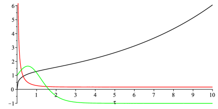
III.1.5 Exponential evolution of
Let us consider, the auxiliary metric function evolve as . In this case, If we solve Eq.(26) with respect to the then the scale factor becomes
| (73) |
where and are the integration constants. Then the Hubble parameter can be found as
| (74) |
the effective equation of state,
| (75) |
In Fig. 1, we demonstrate the time evolution of these parameters in two certain conditions. In both condition, For the late time situations, the scale factor is increasing, the analog of Hubble parameter for is almost remains constant and the EoS function behaves like dark energy ().
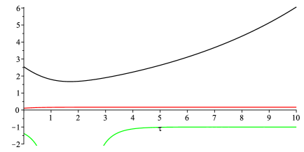
III.1.6 Power-law evolution of
Let us consider, the auxiliary metric function behave as a power-law evolution . In this case, if we solve Eq.(26) with respect to the then the scale factor becomes
| (80) |
and the Hubble parameter,
| (81) |
the effective equation of state,
| (82) |
In Fig. 2, we present the time-dependence of the scale factor and the effective EoS. In the given conditions, for increasing parameters, the scale factor growing rapidly and the EoS shows dark energy like behavior.
III.2 The Parametric Friedmann equations
Having observed that enforcing a conformal Ansatz, typically employed in pure theories, we will now demonstrate an alternative solution to the connection equation. This approach avoids imposing any constraints on the form of the function that defines the gravity Lagrangian. In order to examine the characteristics of the cosmological solutions within the framework of the generalized theory described by Eqs.(5) and (3), we adopt a method akin to the approach suggested in [23] for our specific model. Using the notation and to denote and , respectively. By defining the object , (3) can be written as follows;
| (87) |
where is the identity matrix, and denotes . This equation establishes an algebraic relation between the object and the matter. Now, multiplying this equation by and defining
We can now consider the connection equation (5), which can also be written as
| (90) |
where we have defined
| (91) |
Assuming that is invertible, as will be the case of a perfect fluid to be considered in this work, we can write the term within brackets in the above equation as and look for an auxiliary metric such that thus we can write
| (92) |
The connection equation (90) can thus be written as which implies that is the Levi- Civita connection of .
Raising one index of this equation with and using the definitions of and , we get
| (93) |
III.2.1 Perfect fluid scenarios
For a perfect fluid with energy density , pressure , and stress-energy tensor of the form
| (94) |
we find that
| (95) |
where
| (96) |
| (97) |
By using these results one can find that
| (98) |
| (99) |
where
| (100) |
In this case, if term is negligible or the constant goes to zero we recover the result of the BI case. In this scenario, if the term turns negative, the square root has the potential to reach zero or even take on negative values, which could lead to inconsistencies.
III.2.2 General expressions for and
As mentioned earlier, equations (101) and (102) establish algebraic relationships among the variables , , , and but only two of these variables are truly independent. In this context, obtaining an expression for and in relation to and is quite straightforward, and it doesn’t necessitate specifying the specific Lagrangian. This approach yields and in parametric form. The idea is to start from (101) and transforming it into the following format,
| (103) |
This relation can be inserted in (102) to remove the dependence on or to remove the dependence on . For instance, using (103) to remove the dependence on from (102) and defining , we get
| (104) |
which allows us to write as
| (105) |
A similar approach can be used to extract from
| (106) |
In this case, one gets
| (107) |
The procedure is analogous to the previous case and yields
| (108) |
As was already assumed at the beginning of this section, we focus on a cosmological symmetry and use the unimodular metric in Eq.(10) and use relations (92) to find its relation with the components of necessary to use the field equations (93). Following a notation similar to that used in [59], we can write
| (109) |
which implies
| (110) |
| (111) |
Recall that since and are functions of and , it follows that is a function of time, as we have explicitly written above. This is the only aspect we need to know so far to proceed with the derivation of the Hubble equation. After a bit of algebra, one gets
III.2.3 A model
To illustrate the procedure to deal with the theories presented in this work, we consider a simple model characterized by a function . In order to determine the impact of changing the coefficient in front of the piece from the above action on the Hubble function (114), we need to work out the dependence of and on and using formulas (105) and (108). The first step is to solve from (104). To do so, it is convenient to introduce the redefinition , which turns (104) into
| (115) |
| (116) |
With this definition, one finds that (105) can be written as
| (117) |
The equation for can be manipulated in a very similar way. Introducing the replacement , (108) becomes
| (118) |
which admits the same solution as . Therefore, one finds that (108) can be written as
| (119) |
Thus, using Eqs.(117) and (119), we can write
| (120) |
Taking into account of Eq.(116), this equation establishes a relation between and which is also allow us to show as a function of . To illustrate this point, consider the case which satisfies the conditions the BI theory () and the BI- case without the term (). For an arbitrary can be found such as , the curvature function in terms of can be found as,
| (121) |
which is valid for any .
IV Conclusion
In this paper, we propose a novel modified gravity theory, namely the extension of Born-Infeld- (BI-) gravity, in the context of unimodular gravity. In particular, we first formulate the action corresponding to the generalized BI- gravity, and then, we present a reconstruction scheme of this unimodular extension to achieve various cosmological eras of the universe.
Based on the fact that the determinant of the space-time metric is constrained to be unity in unimodular gravity, we have investigated which metric proves to be compatible with such a constraint since the standard FRW metric is unable to do so. Similar to the standard unimodular theory, it turns out that the constraint on the determinant of the metric can be imposed in the present context by introducing a Lagrange multiplier in the gravitational action. Having formulated the action of the unimodular BI- gravity (that indeed respects the constraint of the metric), we derive the equations of motion by employing the metric formalism. The resulting equations immediately propose a reconstruction method, by which, one can determine the form of unimodular BI- gravity corresponding to some given cosmological evolution. It further opens the avenue to find which cosmological evolution corresponds to a given unimodular BI- gravity. The resulting cosmological scenario seems to be different from the ordinary gravity, as was probably expected. Interestingly, the unimodular generalization of BI- gravity turns out to be suitable for inflation (de-Sitter and quasi de-Sitter) along with power law cosmology which actually includes from reheating to the Standard Big Bang cosmology (depending on the exponent of the power law scale factor). For quasi de-Sitter inflation, we consider the Starobinsky kind of inflation which has an exit, and also, the observable indices (like the spectral index and the tensor-to-scalar ratio) are in agreement with the Planck data. Here it deserves mentioning that in the case of the Starobinsky inflation, the form of in the unimodular BI- theory is different than that of the standard theory. The potential applications of the reconstruction method we present in this paper are quite many since it is possible to realize various cosmological evolutions, which are exotic for the standard Einstein-Hilbert gravity and cannot be realized in that case, for example bouncing cosmologies. In this regard, we show that apart from the inflation, such generalized BI- theory is also capable to trigger non-singular bouncing cosmology for suitable forms of the unimodular Lagrange multiplier. Thus as a whole, we determine the required form of and the unimodular Lagrange multiplier to achieve inflation and the Standard Big Bang evolution of the universe.
However, we would like to mention that we have not described the universe’s evolution as a unified picture. It will be interesting to address the unification of various cosmological eras in the context of unimodular BI- gravity, which we expect to study elsewhere. Also, an issue we did not address in this paper is the cosmological behaviour of BI- near mild singularities, like the Type IV singularity. Therefore, a concrete analysis of the unimodular BI- gravity theory near mild and even crushing types singularities is of some interest and should be appropriately addressed in a future work (for more details about the cosmological singularities, see recent reviews in [60, 61]). Moreover, it is interesting that there exists a mimetic extension of unimodular gravity [62], and by following this approach, one can extend the current theory to mimetic unimodular BI- gravity. It would be of interest to study this question in case of the gravity model under consideration. We also note that the recent review [63] is devoted to the study of modifications of early and late universe descriptions to solve the current cosmic tensions. This will be done elsewhere. We hope to address some of the aforementioned issues in a future work.
Declaration of competing interest
The authors declare no conflicts of interest.
Data Availability Statement
No data was used for the research described in the article.
Acknowledgments
This work was partially supported by MICINN (Spain), project PID2019-104397GB-I00 and by the program Unidad de Excelencia Maria de Maeztu CEX2020-001058-M, Spain (S.D.O).
References
- Guth [1981] A. H. Guth, The Inflationary Universe: A Possible Solution to the Horizon and Flatness Problems, Phys. Rev. D 23, 347 (1981).
- Linde [1990] A. D. Linde, Particle physics and inflationary cosmology, Vol. 5 (1990) arXiv:hep-th/0503203 .
- Langlois [2004] D. Langlois, Inflation, quantum fluctuations and cosmological perturbations, in Cargese School of Particle Physics and Cosmology: the Interface (2004) pp. 235–278, arXiv:hep-th/0405053 .
- Riotto [2003] A. Riotto, Inflation and the theory of cosmological perturbations, ICTP Lect. Notes Ser. 14, 317 (2003), arXiv:hep-ph/0210162 .
- Baumann [2011] D. Baumann, Inflation, in Theoretical Advanced Study Institute in Elementary Particle Physics: Physics of the Large and the Small (2011) pp. 523–686, arXiv:0907.5424 [hep-th] .
- Born and Infeld [1934] M. Born and L. Infeld, Foundations of the new field theory, Proc. Roy. Soc. Lond. A 144, 425 (1934).
- Deser and Gibbons [1998] S. Deser and G. W. Gibbons, Born-Infeld-Einstein actions?, Class. Quant. Grav. 15, L35 (1998), arXiv:hep-th/9803049 .
- Banados and Ferreira [2010] M. Banados and P. G. Ferreira, Eddington’s theory of gravity and its progeny, Phys. Rev. Lett. 105, 011101 (2010), [Erratum: Phys.Rev.Lett. 113, 119901 (2014)], arXiv:1006.1769 [astro-ph.CO] .
- Odintsov et al. [2014] S. D. Odintsov, G. J. Olmo, and D. Rubiera-Garcia, Born-Infeld gravity and its functional extensions, Phys. Rev. D 90, 044003 (2014), arXiv:1406.1205 [hep-th] .
- Du et al. [2014] X.-L. Du, K. Yang, X.-H. Meng, and Y.-X. Liu, Large Scale Structure Formation in Eddington-inspired Born-Infeld Gravity, Phys. Rev. D 90, 044054 (2014), arXiv:1403.0083 [gr-qc] .
- Kim [2014] H.-C. Kim, Origin of the universe: A hint from Eddington-inspired Born-Infeld gravity, J. Korean Phys. Soc. 65, 840 (2014), arXiv:1312.0703 [gr-qc] .
- Kruglov [2014] S. I. Kruglov, Modified arctan-gravity model mimicking a cosmological constant, Phys. Rev. D 89, 064004 (2014), arXiv:1310.6915 [gr-qc] .
- Yang et al. [2013] K. Yang, X.-L. Du, and Y.-X. Liu, Linear perturbations in Eddington-inspired Born-Infeld gravity, Phys. Rev. D 88, 124037 (2013), arXiv:1307.2969 [gr-qc] .
- Avelino and Ferreira [2012] P. P. Avelino and R. Z. Ferreira, Bouncing Eddington-inspired Born-Infeld cosmologies: an alternative to Inflation ?, Phys. Rev. D 86, 041501 (2012), arXiv:1205.6676 [astro-ph.CO] .
- Escamilla-Rivera et al. [2012] C. Escamilla-Rivera, M. Banados, and P. G. Ferreira, A tensor instability in the Eddington inspired Born-Infeld Theory of Gravity, Phys. Rev. D 85, 087302 (2012), arXiv:1204.1691 [gr-qc] .
- Cho et al. [2012] I. Cho, H.-C. Kim, and T. Moon, Universe Driven by Perfect Fluid in Eddington-inspired Born-Infeld Gravity, Phys. Rev. D 86, 084018 (2012), arXiv:1208.2146 [gr-qc] .
- Scargill et al. [2012] J. H. C. Scargill, M. Banados, and P. G. Ferreira, Cosmology with Eddington-inspired Gravity, Phys. Rev. D 86, 103533 (2012), arXiv:1210.1521 [astro-ph.CO] .
- Harko et al. [2014] T. Harko, F. S. N. Lobo, M. K. Mak, and S. V. Sushkov, Dark matter density profile and galactic metric in Eddington-inspired Born–Infeld gravity, Mod. Phys. Lett. A 29, 1450049 (2014), arXiv:1305.0820 [gr-qc] .
- Avelino [2012] P. P. Avelino, Eddington-inspired Born-Infeld gravity: astrophysical and cosmological constraints, Phys. Rev. D 85, 104053 (2012), arXiv:1201.2544 [astro-ph.CO] .
- Olmo et al. [2014] G. J. Olmo, D. Rubiera-Garcia, and H. Sanchis-Alepuz, Geonic black holes and remnants in Eddington-inspired Born-Infeld gravity, Eur. Phys. J. C 74, 2804 (2014), arXiv:1311.0815 [hep-th] .
- Lobo et al. [2014] F. S. N. Lobo, G. J. Olmo, and D. Rubiera-Garcia, Microscopic wormholes and the geometry of entanglement, Eur. Phys. J. C 74, 2924 (2014), arXiv:1402.5099 [hep-th] .
- Harko et al. [2015] T. Harko, F. S. N. Lobo, M. K. Mak, and S. V. Sushkov, Wormhole geometries in Eddington-Inspired Born–Infeld gravity, Mod. Phys. Lett. A 30, 1550190 (2015), arXiv:1307.1883 [gr-qc] .
- Makarenko et al. [2014a] A. N. Makarenko, S. Odintsov, and G. J. Olmo, Born-Infeld- gravity, Phys. Rev. D 90, 024066 (2014a), arXiv:1403.7409 [hep-th] .
- Makarenko et al. [2014b] A. N. Makarenko, S. D. Odintsov, and G. J. Olmo, Little Rip, CDM and singular dark energy cosmology from Born-Infeld- gravity, Phys. Lett. B 734, 36 (2014b).
- Nojiri and Odintsov [2011] S. Nojiri and S. D. Odintsov, Unified cosmic history in modified gravity: from F(R) theory to Lorentz non-invariant models, Phys. Rept. 505, 59 (2011), arXiv:1011.0544 [gr-qc] .
- Nojiri et al. [2017] S. Nojiri, S. D. Odintsov, and V. K. Oikonomou, Modified Gravity Theories on a Nutshell: Inflation, Bounce and Late-time Evolution, Phys. Rept. 692, 1 (2017), arXiv:1705.11098 [gr-qc] .
- Capozziello and De Laurentis [2011] S. Capozziello and M. De Laurentis, Extended Theories of Gravity, Phys. Rept. 509, 167 (2011), arXiv:1108.6266 [gr-qc] .
- Nojiri and Odintsov [2014] S. Nojiri and S. D. Odintsov, Accelerating cosmology in modified gravity: from convenient or string-inspired theory to bimetric gravity, Int. J. Geom. Meth. Mod. Phys. 11, 1460006 (2014), arXiv:1306.4426 [gr-qc] .
- de la Cruz-Dombriz and Saez-Gomez [2012] A. de la Cruz-Dombriz and D. Saez-Gomez, Black holes, cosmological solutions, future singularities, and their thermodynamical properties in modified gravity theories, Entropy 14, 1717 (2012), arXiv:1207.2663 [gr-qc] .
- Finkelstein et al. [2001] D. R. Finkelstein, A. A. Galiautdinov, and J. E. Baugh, Unimodular relativity and cosmological constant, J. Math. Phys. 42, 340 (2001), arXiv:gr-qc/0009099 .
- Alvarez [2005] E. Alvarez, Can one tell Einstein’s unimodular theory from Einstein’s general relativity?, JHEP 03, 002, arXiv:hep-th/0501146 .
- Abbassi and Abbassi [2008] A. H. Abbassi and A. M. Abbassi, Density-metric unimodular gravity: Vacuum spherical symmetry, Class. Quant. Grav. 25, 175018 (2008), arXiv:0706.0451 [gr-qc] .
- Ellis et al. [2011] G. F. R. Ellis, H. van Elst, J. Murugan, and J.-P. Uzan, On the Trace-Free Einstein Equations as a Viable Alternative to General Relativity, Class. Quant. Grav. 28, 225007 (2011), arXiv:1008.1196 [gr-qc] .
- Jain [2012] P. Jain, A flat space-time model of the Universe, Mod. Phys. Lett. A 27, 1250201 (2012), arXiv:1209.2314 [astro-ph.CO] .
- SINGH [2013] N. K. SINGH, Unimodular constraint on global scale invariance, Modern Physics Letters A 28, 1350130 (2013).
- Kluson [2015] J. Kluson, Canonical Analysis of Unimodular Gravity, Phys. Rev. D 91, 064058 (2015), arXiv:1409.8014 [hep-th] .
- Padilla and Saltas [2015] A. Padilla and I. D. Saltas, A note on classical and quantum unimodular gravity, Eur. Phys. J. C 75, 561 (2015), arXiv:1409.3573 [gr-qc] .
- Barceló et al. [2014] C. Barceló, R. Carballo-Rubio, and L. J. Garay, Unimodular gravity and general relativity from graviton self-interactions, Phys. Rev. D 89, 124019 (2014), arXiv:1401.2941 [gr-qc] .
- Barceló et al. [2018] C. Barceló, R. Carballo-Rubio, and L. J. Garay, Absence of cosmological constant problem in special relativistic field theory of gravity, Annals Phys. 398, 9 (2018), arXiv:1406.7713 [gr-qc] .
- Burger et al. [2015] D. J. Burger, G. F. Ellis, J. Murugan, and A. Weltman, The klt relations in unimodular gravity, arXiv preprint arXiv:1511.08517 (2015), arXiv:1511.08517 [hep-th] .
- Álvarez et al. [2015] E. Álvarez, S. González-Martín, M. Herrero-Valea, and C. P. Martín, Quantum Corrections to Unimodular Gravity, JHEP 08, 078, arXiv:1505.01995 [hep-th] .
- Jain et al. [2012a] P. Jain, A. Jaiswal, P. Karmakar, G. Kashyap, and N. K. Singh, Cosmological implications of unimodular gravity, JCAP 11, 003, arXiv:1109.0169 [astro-ph.CO] .
- Alvarez and Velasco-Aja [2023] E. Alvarez and E. Velasco-Aja, A Primer on Unimodular Gravity (2023) arXiv:2301.07641 [gr-qc] .
- Jain et al. [2012b] P. Jain, P. Karmakar, S. Mitra, S. Panda, and N. K. Singh, Testing Unimodular Gravity, JCAP 05, 020, arXiv:1108.1856 [gr-qc] .
- Nojiri et al. [2016a] S. Nojiri, S. D. Odintsov, and V. K. Oikonomou, Unimodular Gravity, JCAP 05, 046, arXiv:1512.07223 [gr-qc] .
- Nojiri et al. [2016b] S. Nojiri, S. D. Odintsov, and V. K. Oikonomou, Newton law in covariant unimodular gravity, Mod. Phys. Lett. A 31, 1650172 (2016b), arXiv:1605.00993 [gr-qc] .
- Nojiri et al. [2016c] S. Nojiri, S. D. Odintsov, and V. K. Oikonomou, Bounce universe history from unimodular gravity, Phys. Rev. D 93, 084050 (2016c), arXiv:1601.04112 [gr-qc] .
- Beltran Jimenez et al. [2018] J. Beltran Jimenez, L. Heisenberg, G. J. Olmo, and D. Rubiera-Garcia, Born–Infeld inspired modifications of gravity, Phys. Rept. 727, 1 (2018), arXiv:1704.03351 [gr-qc] .
- Guth [2007] A. H. Guth, Eternal inflation and its implications, J. Phys. A 40, 6811 (2007).
- Akrami et al. [2020] Y. Akrami et al. (Planck), Planck 2018 results. X. Constraints on inflation, Astron. Astrophys. 641, A10 (2020), arXiv:1807.06211 [astro-ph.CO] .
- Starobinsky [1980] A. A. Starobinsky, A New Type of Isotropic Cosmological Models Without Singularity, Phys. Lett. B 91, 99 (1980).
- Barrow and Cotsakis [1988] J. D. Barrow and S. Cotsakis, Inflation and the Conformal Structure of Higher Order Gravity Theories, Phys. Lett. B 214, 515 (1988).
- Odintsov and Oikonomou [2015a] S. D. Odintsov and V. K. Oikonomou, Bouncing cosmology with future singularity from modified gravity, Phys. Rev. D 92, 024016 (2015a).
- Odintsov and Oikonomou [2015b] S. D. Odintsov and V. K. Oikonomou, Singular Inflationary Universe from Gravity, Phys. Rev. D 92, 124024 (2015b).
- Koehn et al. [2014] M. Koehn, J.-L. Lehners, and B. A. Ovrut, Cosmological super-bounce, Phys. Rev. D 90, 025005 (2014).
- Odintsov et al. [2015] S. D. Odintsov, V. K. Oikonomou, and E. N. Saridakis, Superbounce and Loop Quantum Ekpyrotic Cosmologies from Modified Gravity: , and Theories, Annals Phys. 363, 141 (2015).
- Oikonomou [2015] V. K. Oikonomou, Superbounce and Loop Quantum Cosmology Ekpyrosis from Modified Gravity, Astrophys. Space Sci. 359, 30 (2015).
- Odintsov and Paul [2022] S. D. Odintsov and T. Paul, Bounce Universe with Finite-Time Singularity, Universe 8, 292 (2022), arXiv:2205.09447 [gr-qc] .
- Olmo and Olmo [2012] G. J. Olmo and G. J. Olmo, eds., Open Questions in Cosmology (InTech, 2012).
- de Haro et al. [2023] J. de Haro, S. Nojiri, S. D. Odintsov, V. K. Oikonomou, and S. Pan, Finite-time cosmological singularities and the possible fate of the Universe, Phys. Rept. 1034, 1 (2023).
- Trivedi [2023] O. Trivedi, Recent advances in cosmological singularities, arXiv preprint (2023), arXiv:2309.08954 [gr-qc] .
- Nojiri et al. [2016d] S. Nojiri, S. D. Odintsov, and V. K. Oikonomou, Unimodular-Mimetic Cosmology, Class. Quant. Grav. 33, 125017 (2016d), arXiv:1601.07057 [gr-qc] .
- Vagnozzi [2023] S. Vagnozzi, Seven Hints That Early-Time New Physics Alone Is Not Sufficient to Solve the Hubble Tension, Universe 9, 393 (2023).