Unraveling the emergence of quantum state designs in systems with symmetry

Abstract

Quantum state designs, by enabling an efficient sampling of random quantum states, play a quintessential role in devising and benchmarking various quantum protocols with broad applications ranging from circuit designs to black hole physics. Symmetries, on the other hand, are expected to reduce the randomness of a state. Despite being ubiquitous, the effects of symmetry on the quantum state designs remain an outstanding question. The recently introduced projected ensemble framework generates efficient approximate state $t$-designs by hinging on projective measurements and many-body quantum chaos. In this work, we examine the emergence of state designs from the random generator states exhibiting symmetries. Leveraging on translation symmetry, we analytically establish a sufficient condition for the measurement basis leading to the state $t$-designs. Then, by making use of a trace distance measure, we numerically investigate the convergence to the designs. Subsequently, we inspect the violation of the sufficient condition to identify bases that fail to converge. We further demonstrate the emergence of state designs in a physical system by studying dynamics of a chaotic tilted field Ising chain with periodic boundary conditions. We find faster convergence of the trace distance in the initial time, however, it saturates to a finite value deviating from random matrix prediction at late time, in contrast to the case with open boundary condition. To delineate the general applicability of our results, we extend our analysis to other symmetries. We expect our findings to pave the way for further exploration of deep thermalization and equilibration of closed and open quantum many-body systems.

I Introduction

Preparing random quantum states and operators is an essential ingredient to explore a variety of quantum protocols, such as randomized benchmarking Emerson et al. (2005); Knill et al. (2008); Dankert et al. (2009), randomized measurements Vermersch et al. (2019); Elben et al. (2023), circuit designs Harrow and Low (2009); Brown and Viola (2010), quantum state tomography Smith et al. (2013); Merkel et al. (2010), etc., and has vast applications ranging from quantum gravity Sekino and Susskind (2008), information scrambling Styliaris et al. (2021); Hosur et al. (2016), quantum chaos Haake (1991), information recovery Hayden and Preskill (2007); Yoshida and Kitaev (2017), machine-learning Huang et al. (2020, 2022); Holmes et al. (2021) to quantum algorithms Tilly et al. (2022). Quantum state $t$-designs were introduced to answer the pertinent question: How can one efficiently sample a Haar random state from the given Hilbert space? To this end, state designs correspond to finite ensembles of pure states uniformly distributed over the Hilbert space, replicating the behavior of Haar random states to a certain degree Renes et al. (2004); Klappenecker and Rotteler (2005); Dankert et al. (2009). However, generating such states in experiments is a challenging task since it requires precise control over the targeted degrees of freedom with fine-tuned resolution Morvan et al. (2021); Proctor et al. (2022); Boixo et al. (2018).

Motivated by the recent advances in quantum technologies Gross and Bloch (2017); Blatt and Roos (2012); Browaeys et al. (2016); Gambetta et al. (2017), the ‘projected ensemble’ framework has been introduced as a natural avenue for the emergence of state designs from quantum chaotic dynamics Cotler et al. (2023); Choi et al. (2023). Under this framework, one employs projective measurements on the larger subsystem (bath) of a single bi-partite state undergoing quantum chaotic evolution, which generates a set of pure states on the smaller subsystem. These states, together with the Born probabilities, referred to as the projected ensemble, remarkably converge to a state design when the measured part of the system is sufficiently large. This phenomenon, dubbed as emergent state design, has been closely tied to a stringent generalization of regular quantum thermalization. Under the usual framework, predominately characterized through the Eigenstate Thermalization Hypothesis (ETH) Deutsch (1991); Srednicki (1994); Rigol et al. (2008); D’Alessio et al. (2016); Deutsch (2018); Roy et al. (2023), the bath degrees of freedom are traced out and the thermalization is retrieved at level of local observables. Whereas, the projected ensemble retains the memory of the bath through the measurements such that thermalization is exlplored for the sub-system wavefunctions. This generalization has been referred to as deep thermalization Ho and Choi (2022); Ippoliti and Ho (2022, 2023). The emergence of higher-order state designs has been explicitly studied in recent years under various physical settings Cotler et al. (2023); Ho and Choi (2022); Ippoliti and Ho (2022); Lucas et al. (2023); Shrotriya and Ho (2023); Versini et al. (2023), including dual unitary circuits Claeys and Lamacraft (2022); Ippoliti and Ho (2023) and constrained physical models Bhore et al. (2023) with applications to classical shadow tomography McGinley and Fava (2023) and benchmarking quantum devices Choi et al. (2023). In the case of chaotic systems without symmetries, arbitrary measurement bases can be considered to witness the emergence of state designs. The presence of symmetries is expected to influence this property.

Symmetries in quantum systems are associated with discrete or continuous group structures. Their presence causes the decomposition of the system into charge-conserving subspaces. This results in constraining the dynamical Khemani et al. (2018); Rakovszky et al. (2018); Friedman et al. (2019) and equilibrium properties Yunger Halpern et al. (2016) of many-body systems Nakata et al. (2023); Bhattacharya et al. (2017); Balachandran et al. (2021); Kudler-Flam et al. (2022); Chen et al. (2020); Paviglianiti et al. (2023); Agarwal et al. (2023); Varikuti and Madhok (2022). When a generic system displays symmetry, ETH is known to be satisfied within each invariant subspace Deutsch (1991); Srednicki (1994); D’Alessio et al. (2016). Deep thermalization, on the other hand, depends non-trivially on the specific measurement basis Cotler et al. (2023); Bhore et al. (2023). Motivated by this, here we ask the intriguing question: What’s the general choice of measurement basis for the emergence of $t$-designs when the generator state abides by a symmetry? In order to address this question, we first adhere our analysis to generator states with translation symmetry. In particular, we consider the ensembles of the random translation invariant (or shortly T-invariant) states, and investigate the emergent state designs within the projected ensemble framework. We then elucidate the generality of our findings by extending its applicability to other discrete symmetries.

This paper is structured as follows. In Sec. II, we briefly review the projected ensemble framework, outline the central question we are trying to address, and summarize our key results. In Sec. III, we consider the ensembles of translation symmetric states and provide an analytical expression for their moments. In Sec. IV.1 and IV.2, we study the emergence of first and higher-order state designs, respectively, and outline a sufficient condition on the measurement basis for achieving these designs. This is followed by an analysis of the violation of the condition shown by various measurement bases in Sec. IV.3. We then consider a chaotic Ising chain with periodic boundary conditions in Sec. V and examine deep thermalization in a state evolved under this Hamiltonian. In Sec. VI, we generalize the results to other discrete symmetries such as $Z_{2}$ and reflection symmetries. Finally, we conclude this paper in Sec. VII.

II Framework and results

Here, we briefly outline the projected ensemble framework Ho and Choi (2022); Cotler et al. (2023) and summarize our main results. A $t$-th order quantum state design ($t$-design) is an ensemble of pure quantum states that reproduces the average behavior of any quantum state polynomial of order $t$ or less over all possible pure states, represented by the Haar average. An ensemble $\mathcal{E}\equiv\{p_{i},|\psi_{i}\rangle\}$ is an exact $t$-design if and only if its moments match those of the Haar ensemble up to order $t$, i.e.,

$$\sum_{i=1}^{|\mathcal{E}|}p_{i}\left(|\psi\rangle\langle\psi|\right)^{\otimes t}=\int_{|\psi\rangle}d\psi\left(|\psi\rangle\langle\psi|\right)^{\otimes t}$$ (1)

The projected ensemble framework aims to generate quantum state designs from a single chaotic or random many-body quantum state. The protocol involves performing local projective measurements on part of the system. First, consider a generator quantum state $|\psi\rangle\in\mathcal{H}^{\otimes N}$, where $\mathcal{H}$ denotes the local Hilbert space of dimension $d$ and $N=N_{A}+N_{B}$ denotes the size of the system constituting subsystems-$A$ and $B$. Then, projectively measuring the subsystem-$B$ gives a statistical mixture of pure states (or projected ensemble) corresponding to the subsystem-$A$. To be more precise, projective measurement of $|\psi\rangle$ in a basis $\mathcal{B}\equiv\{|b\rangle\}$ supported over the subsystem-$B$ yielding the state

$$|\tilde{\psi}(b)\rangle=\left(\mathbb{I}_{2^{N_{A}}}\otimes|b\rangle\langle b|\right)|\psi\rangle\quad\text{ (unnormalized) },$$ (2)

with the probability $p_{b}=\langle\tilde{\psi}(b)|\tilde{\psi}(b)\rangle=\langle\psi|b\rangle\langle b|\psi\rangle$. Since the projective measurements result in disentangling the subsystems, we can safely disregard the subsystem-$B$ and focus on the quantum state of subsystem-$A$. After normalizing the post-measurement state, we obtain

$$|\phi(b)\rangle=\dfrac{|\tilde{\psi}(b)\rangle}{\sqrt{p_{b}}}=\dfrac{\left(\mathbb{I}_{2^{N_{A}}}\otimes\langle b|\right)|\psi\rangle}{\sqrt{\langle\psi|b\rangle\langle b|\psi\rangle}}.$$ (3)

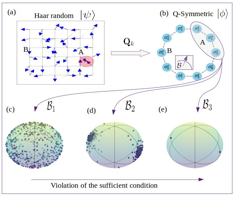
Figure 1: Schematic representation of the projected ensemble framework for a $Q$-symmetric state (an eigenstate of a symmetry operator $Q$), showcasing the interplay between measurement bases and symmetry. (a) Haar random state, wherein the spins are randomly aligned and entangled. An application of the subspace projector $Q_{k}$ takes the Haar random state to an invariant subspace with charge $k$, which is depicted in (b). For simplicity, we are showing a $Z_{2}$ symmetric state (see Sec. VI.1) in this schematic. The labels $\sigma^{x}_{j}$ indicate that the state is invariant under spin-flip operations. The resultant state is subjected to projective measurements over the subsystem-$B$. These measurements result in the so-called projected ensembles supported over $A$ (see Sec. II). (c)-(d) distributions of the resultant projected ensembles for three different measurement bases. While in (c), the measurements in $\mathcal{B}_{1}$ yield a uniformly distributed projected ensemble, $\mathcal{B}_{2}$ and $\mathcal{B}_{3}$ result in ensembles of pure states localized near $|\pm\rangle$ states. We understand that the latter cases largely violate a sufficient condition we derive in this text for the emergence of state designs.

Then, the projected ensemble on $A$ given by $\mathcal{E}(|\psi\rangle,\mathcal{B})\equiv\left\{p_{b},|\phi(b)\rangle\right\}$ approximate higher-order quantum state designs if $|\psi\rangle$ is generated by a chaotic evolution Ho and Choi (2022); Cotler et al. (2023), i.e., for $t\geq 1$,

$$\Delta^{(t)}_{\mathcal{E}}\equiv\left\|\sum_{|b\rangle\in\mathcal{B}}\dfrac{\left(\langle b|\psi\rangle\langle\psi|b\rangle\right)^{\otimes t}}{\left(\langle\psi|b\rangle\langle b|\psi\rangle\right)^{t-1}}-\int_{\phi\in\mathcal{E}^{A}_{\text{Haar}}}d\phi\left[|\phi\rangle\langle\phi|\right]^{\otimes t}\right\|_{1}\leq\varepsilon.$$ (4)

In the above equation, the trace norm (or Schatten $1$-norm) of an operator $W$, denoted as $\|W\|_{1}$, is defined as $\|W\|_{1}=\Tr(\sqrt{W^{\dagger}W})$, which is equivalent to the sum of singular values of the operator. The two terms inside the trace norm are the $t$-th moments of the projected ensemble and the ensemble of Haar random states supported over $A$, respectively. It is important to note that Renes et al. (2004)

$$\int_{|\phi\rangle\in\mathcal{E}^{A}_{\text{Haar}}}d\phi\left(|\phi\rangle\langle\phi|\right)^{\otimes t}=\dfrac{\bm{\Pi}^{A}_{t}}{\mathcal{D}_{A}},$$ (5)

where the Haar measure over $\mathcal{E}^{A}_{\text{Haar}}$ is denoted by $d\phi$, $\mathcal{D}_{A}=d^{N_{A}}(d^{N_{A}}+1)\cdots(d^{N_{A}}+t-1)$, and $\bm{\Pi}^{A}_{t}$ is the projector onto the permutation symmetric subspace of the Hilbert space $\mathcal{H}^{\otimes N_{A}}\otimes\mathcal{H}^{\otimes N_{A}}\otimes\cdots t$-times, i.e., $\bm{\Pi}^{A}_{t}=\sum_{\pi_{i}\in S_{t}}\pi_{i}$. The permutation group is represented by $S_{t}$. The permutation operators $\pi_{i}$’s act on $t$-replicas of the same Hilbert space ($\mathcal{H}^{\otimes N_{A}}$) as follows:

$$\pi_{i}\left(|\psi_{1}\rangle\otimes...\otimes|\psi_{t}\rangle\right)=|\psi_{{\pi}^{-1}(1)}\rangle\otimes...\otimes|\psi_{{\pi}^{-1}(t)}\rangle.$$ (6)

The trace distance $\Delta^{(t)}_{\mathcal{E}}$ in Eq. (4) vanishes if and only if the ensemble $\mathcal{E}(|\psi\rangle,\mathcal{B})$ forms an exact $t$-design Renes et al. (2004); Klappenecker and Rotteler (2005); Dankert et al. (2009). If the generator state $|\psi\rangle$ is Haar random, the trace distance $\Delta^{(t)}_{\mathcal{E}}$ exponentially converges to zero with $N_{B}$ for any $t\geq 1$, as demonstrated in Ref. Cotler et al. (2023). In this case, the measurement basis can be arbitrary, and the behavior is generic to the choice of basis. On the other hand, for the generator state abiding by symmetry, the choice of measurement basis becomes crucial. In this work, we address this particular aspect.

Our general result can be summarized as follows: Given a symmetry operator $Q$ and a measurement basis $\mathcal{B}$, the projected ensembles of generic $Q$-symmetric quantum states approximate state $t$-designs if for all $|b\rangle\in\mathcal{B}$, $\langle b|\mathbf{Q}_{k}|b\rangle=\mathbb{I}_{2^{N_{A}}}$, where $\mathbf{Q}_{k}$ represents the projector onto an invariant subspace with charge $k$. Here, it is to be noted that $\mathbf{Q}_{k}$ can be constructed by taking an appropriate linear combination of the elements of the corresponding symmetry group. We employ $\Delta^{t}_{\mathcal{E}}$ as a figure of merit for the state designs. We explicitly derive this condition for the ensembles of translation invariant states and provide arguments to show its generality to other symmetries. We further elucidate the emergence of state designs from translation symmetric states by explicitly considering a physical model.

III T-invariant quantum states

In this section, we construct the ensembles of translation symmetric (T-invariant) quantum states from the Haar random states and calculate the moments associated with those ensembles. The T-invariant states are well studied in condensed matter physics and quantum field theory for the ground state properties, such as entanglement and phase transitions. Due to the non-onsite nature of the symmetry, the generic T-invariant states (excluding the product states of the form $|\psi\rangle^{\otimes N}$) are necessarily long-range entangled Gioia and Wang (2022). Thus, in a generic T-invariant state, the information is uniformly spread across all the sites, somewhat mimicking the Haar random states. This makes them ideal candidates for generating state designs besides Haar random states. Moreover, in the context of ETH, generic T-invariant systems have been shown to thermalize local observables Santos and Rigol (2010); Mori et al. (2018); Sugimoto et al. (2023). Hence, studying deep thermalization in these systems is of profound interest.

Let $T=e^{iP}$ denote the lattice translation operator on a system with a total of $N$ sites, each having a local Hilbert space dimension of $d$, where $P$ is the lattice momentum operator. Then, $T$ can be defined by its action on the computational basis vectors as follows:

$$T|i_{1},i_{2},...,i_{N}\rangle=|i_{N},i_{1},...,i_{N-1}\rangle,$$ (7)

with $N$-th roots of unity as eigenvalues. A system is considered T-invariant if its Hamiltonian $H$ commutes with $T$, i.e., $[H,T]=0$. A T-invariant state $|\psi\rangle$ is an eigenstate of $T$ with an eigenvalue $e^{-2\pi ik/N}$, i.e., $T|\psi\rangle=e^{-2\pi ik/N}|\psi\rangle$, where $k\in\mathbb{Z}_{\geq 0}$ and $0\leq k\leq N-1$, characterizes the lattice momentum charge. We then represent the set of all pure T-invariant states having the momentum charge $k$ with $\mathcal{E}^{k}_{\text{TI}}$. To compute their moments, we first outline their construction from the Haar random states, followed by the Haar average.

The translation operator, $T$, generates the translation group given by $\{T^{j}\}_{j=0}^{N-1}$. Then, a Haar random state $|\psi\rangle\in\mathcal{H}^{\otimes N}$ can be projected onto a translation symmetric subspace by taking a uniform superposition of the states $\{e^{2\pi ijk/N}T^{j}|\psi\rangle\}_{j=0}^{N-1}$:

$$|\psi\rangle\rightarrow|\phi\rangle=\mathbb{T}_{k}(|\psi\rangle)=\dfrac{1}{\mathcal{N}}\mathbf{T}_{k}|\psi\rangle,$$ (8)

where

$$\mathbf{T}_{k}=\sum_{j=0}^{N-1}e^{2\pi ijk/N}T^{j}\quad\text{and }\mathcal{N}=\sqrt{\langle\psi|\mathbf{T}^{\dagger}_{k}\mathbf{T}_{k}|\psi\rangle}.$$ (9)

Here, the mapping from $|\psi\rangle$ to the T-invariant state $|\phi\rangle$ is denoted with $\mathbb{T}_{k}(|\psi\rangle)$. The Hermitian operator $\mathbf{T}_{k}$ projects any generic state onto an invariant momentum sector with the charge $k$. Therefore, $\mathbf{T}_{k}\mathbf{T}_{k^{\prime}}=N\mathbf{T}_{k}\delta_{k,k^{\prime}}$, yielding the normalizing factor $\mathcal{N}=\sqrt{N\langle\psi|\mathbf{T}_{k}|\psi\rangle}$. The resultant state $|\phi\rangle$ is an eigenstate of $T$ with the eigenvalue $e^{-2\pi ik/N}$, i.e., $T|\phi\rangle=e^{-2\pi ik/N}|\phi\rangle$. In this way, one can project the set of Haar random states to an $N$-number of disjoint sets of random T-invariant states, each characterized by the momentum charge $k$. Introducing the translation invariance causes partial de-randomization of the Haar random states. This is because a generic quantum state with support over $N$ sites can be described using $n_{\text{Haar}}\approx d^{N}$ independent complex parameters Linden et al. (1998). The translation invariance, however, reduces this number by a factor of $N$, i.e., $n_{\text{TI}}\approx d^{N}/N$. As we shall see, this results in more structure of the moments of the T-invariant states, $\mathbb{E}_{\phi\in\mathcal{E}^{k}_{\text{TI}}}\left[|\phi\rangle\langle\phi|^{\otimes t}\right]$.

Before evaluating the moments of $\mathcal{E}^{k}_{\text{TI}}$, it is useful to state the following result:

Result III.1.

Let $U_{\text{TI}}(d^{N})$ be a subset of the unitary group $U(d^{N})$, which contains all the unitaries that are T-invariant, i.e., $[v,T]=0$ for all $v\in U_{\text{TI}}(d^{N})$, then $U_{\text{TI}}(d^{N})$ is a compact subgroup of $U(d^{N})$.

Proof.

Consider the subset $U_{\text{TI}}(d^{N})$ of $U(d^{N})$ containing all the T-invariant unitaries — for every $v\in U_{\text{TI}}(d^{N})$, we have $T^{\dagger}vT=v$. Clearly, $U_{\text{TI}}(d^{N})$ is a subgroup of $U(d^{N})$. As the operator norm of any unitary matrix is bounded, $U_{\text{TI}}(d^{N})$ is bounded. Moreover, one can define $U_{\text{TI}}(d^{N})$ as the preimage of the null matrix $\mathbf{0}$ under the operation $v-T^{\dagger}vT$ for $v\in U(d^{N})$, hence it is necessarily closed. This implies that $U_{\text{TI}}(d^{N})$ is a compact subgroup of $U(d^{N})$. $\blacksquare$

A method for constructing random translation invariant unitaries using the polar decomposition is outlined in Appendix A. An immediate consequence of the above result is that there exists a natural Haar measure on the subgroup $U_{\text{TI}}(d^{N})$. It is to be noted that projecting Haar random states onto T-invariant subspaces creates uniformly random states within those subspaces. To see this, sample $|\phi\rangle$ and $|\phi^{\prime}\rangle$ from $\mathcal{E}^{k}_{\text{TI}}$ such that they are related to each other via the left invariance of the Haar measure over $U(d^{N})$, i.e., $|\phi\rangle=\mathbf{T}_{k}u|0\rangle/\mathcal{N}$ and $|\phi^{\prime}\rangle=\mathbf{T}_{k}vu|0\rangle/\mathcal{N}$, where $u\in U(d^{N})$ and $v\in U_{\text{TI}}(d^{N})$. Since $v$ and $\mathbf{T}_{k}$ commute, one can write $|\phi^{\prime}\rangle=v|\phi\rangle$. Let $v$ be sampled according to the Haar measure in $U_{\text{TI}}(d^{N})$, then, the state $v|\phi\rangle$ must be uniformly random in $\mathcal{E}^{k}_{\text{TI}}$. Now, $|\phi\rangle$ and $|\phi^{\prime}\rangle$ being sampled through the projection of $\mathbf{T}_{k}$, we can conclude that all the states similarly projected to $\mathcal{E}^{k}_{\text{TI}}$ will be uniformly random. We use this result to derive the moments of $\mathcal{E}^{k}_{\text{TI}}$.

Result III.2.

Let $|\psi\rangle$ be a pure quantum state drawn uniformly at random from the Haar ensemble, then for the mapping $|\psi\rangle\rightarrow|\phi\rangle=\mathbb{T}_{k}(|\psi\rangle)$, it holds that

$$\mathbb{E}_{|\phi\rangle\in\mathcal{E}^{k}_{\text{TI}}}\left[\left[|\phi\rangle\langle\phi|\right]^{\otimes t}\right]=\dfrac{1}{\alpha_{t}}\mathbf{T}^{\otimes t}_{k}\bm{\Pi}_{t},$$ (10)

where $\alpha_{t}$ denotes the normalizing constant, which is given by

$$\alpha_{t}=\Tr\left(\mathbf{T}^{\otimes t}_{k}\bm{\Pi}_{t}\right).$$ (11)

The proof of this result is given in Appendix B. Therefore, the T-invariance imposes an additional structure to the moments through the product of $\mathbf{T}^{\otimes t}_{k}$, where the Haar moments are uniform linear combinations of the permutation group elements. In the following section, we identify a sufficient condition for obtaining approximate state designs from the generic T-invariant generator states sampled from $\mathcal{E}^{k}_{\text{TI}}$.

IV Quantum state designs from T-invariant generator states

In this section, we construct the projected ensembles from the T-invariant generator states sampled from $\mathcal{E}^{k}_{\text{TI}}$and verify their convergence to the quantum state designs. In particular, if $|\phi\rangle$ is drawn uniformly at random from $\mathcal{E}^{k}_{\text{TI}}$, we intend to verify the following identity:

$$\mathbb{E}_{|\phi\rangle\in\mathcal{E}^{k}_{\text{TI}}}\left(\sum\limits_{|b\rangle\in\mathcal{B}}\dfrac{\left(\langle b|\phi\rangle\langle\phi|b\rangle\right)^{\otimes t}}{\left(\langle\phi|b\rangle\langle b|\phi\rangle\right)^{t-1}}\right)=\dfrac{\bm{\Pi}^{A}_{t}}{\mathcal{D}_{A,t}},$$ (12)

where $\mathcal{D}_{A,t}=2^{N_{A}}(2^{N_{A}}+1)...(2^{N_{A}}+t-1)$.

The term on the left-hand side evaluates the $t$-th moment of the projected ensemble of a T-invariant state $|\phi\rangle$, with an average taken over all such states in $\mathcal{E}^{k}_{\text{TI}}$. It has been shown that for the Haar random states, the $t$-th moments of the projected ensembles are Lipshitz continuous functions with a Lipschitz constant $\eta=2(2t-1)$ Cotler et al. (2023). Being $\mathcal{E}^{k}_{\text{TI}}\subset\mathcal{E}_{\text{Haar}}$, $\eta$ is also a Lipschitz constant for the case of $\mathcal{E}^{k}_{\text{TI}}$. Note that the number of independent parameters of a T-invariant state with momentum $k$ is $l=2\rank(\mathbf{T}_{k})-1$. Since $\mathbf{T}_{k}$ is a subspace projector, its eigenvalues assume values either $N$ or zero. Therefore, $\rank(\mathbf{T}_{k})=\Tr(\mathbf{T}_{k})/N$. Hence, a random T-invariant state can be regarded as a point on a hypersphere of dimension $l=2\Tr(\mathbf{T}_{k})/N-1$. As a consequence, if the above relation in Eq. (12) holds, Levy’s lemma guarantees that any typical state drawn from $\mathcal{E}^{k}_{\text{TI}}$ will form an approximate state design. In the following, we first verify the identity in Eq. (12) for $t=1$, followed by the more general case of $t>1$. We then compare the results against the Haar random generator states.

IV.1 Emergence of first-order state designs ($t=1$)

From Eq. (11) of the last section, the first moment of $\mathcal{E}^{k}_{\text{TI}}$ is $\mathbb{E}_{|\phi\rangle\in\mathcal{E}^{k}_{\text{TI}}}\left(|\phi\rangle\langle\phi|\right)=\mathbf{T}_{k}/\alpha^{1}_{k}$, where $\alpha^{1}_{k}$ typically scales exponentially with $N$. If $N$ is a prime number, one can write $\alpha^{1}_{k}$ explicitly as follows Nakata and Murao (2020):

$$\alpha^{1}_{k}=\Tr(\mathbf{T}_{k})=\begin{cases}d^{N}+d(N-1)&\quad\textrm{if }k=0\\ d^{N}-d&\textrm{otherwise. }\end{cases}$$ (13)

To construct the projected ensembles, we now perform the local projective measurements on the $B$-subsystem. For $t=1$, the measurement basis is irrelevant. Then, for some generator state $|\phi\rangle\in\mathcal{E}^{k}_{\text{TI}}$, the first moment of the projected ensemble is given by $\sum_{|b\rangle\in\mathcal{B}}\langle b|\phi\rangle\langle\phi|b\rangle=\Tr_{B}(|\phi\rangle\langle\phi|)$. Typically $\Tr_{B}(|\phi\rangle\langle\phi|)$ approximates the maximally mixed state in the reduced Hilbert space $\mathcal{H}^{\otimes N_{A}}$. We verify this by averaging the partial trace over the ensemble $\mathcal{E}^{k}_{\text{TI}}$:

$$\mathbb{E}_{\phi\in\mathcal{E}^{k}_{\text{TI}}}\left[\Tr_{B}\left(|\phi\rangle\langle\phi|\right)\right] =\Tr_{B}\left[\mathbb{E}_{|\phi\rangle\in\mathcal{E}^{k}_{\text{TI}}}\left(|\phi\rangle\langle\phi|\right)\right]$$

$$=\dfrac{\Tr_{B}(\mathbf{T}_{k})}{{\alpha^{1}_{k}}}.$$ (14)

To examine the closeness of $\Tr_{B}(\mathbf{T}_{k})/\alpha^{1}_{k}$ to the maximally mixed state, we first expand $\mathbf{T}_{k}$ given in Eq. (9) as

$$\Tr_{B}(\mathbf{T}_{k})=2^{N}\left[\dfrac{\mathbb{I}_{A}}{2^{N_{A}}}+\dfrac{1}{2^{N}}\sum_{j=1}^{N-1}e^{2\pi ijk/N}\Tr_{B}(T^{j})\right].$$ (15)

For $j=1$, it can be shown that $\Tr_{B}(T)=T_{A}$, where $T_{A}$ is the translation operator acting exclusively on the subsystem-$A$. For $j\geq 2$, $\Tr_{B}(T^{j})=\sum_{b}\langle b|T^{j}|b\rangle$ outputs a random permutation operator supported over $A$ whenever $N_{A}\geq\gcd{(N,j)}$. If $N_{A}<\gcd{(N,j)}$, the partial trace would result in a constant times identity operator $\mathbb{I}_{2^{N_{A}}}$. Interested readers can find more details in Appendix C. If $N$ is prime and $2\leq j<N$, we have $\gcd{(N,j)}=1$, which is less than $N_{A}$ whenever $N_{A}>2$. Then, one can explicitly show that the trace norm of the second term on the right side in Eq. (15) is bounded from above as follows:

$$\dfrac{1}{2^{N}}\left\|\sum_{j=1}^{N-1}e^{2\pi ijk/N}\Tr_{B}(T^{j})\right\|_{1}\leq\sum_{j=1}^{N-1}\dfrac{\left\|\Tr_{B}(T^{j})\right\|_{1}}{2^{N}}=\dfrac{(N-1)}{2^{N_{B}}},$$ (16)

implying that it converges to a null matrix exponentially with $N_{B}$. Hence, Eq. (IV.1) converges exponentially with $N_{B}$ to the maximally mixed state ($\rho_{A}\propto\mathbb{I}$) in the reduced Hilbert space $\mathcal{H}^{\otimes N_{A}}$ — for $N_{B}\gg\log_{2}(N)$, we have $\mathbb{E}_{\phi}[\sum_{b}\langle b|\phi\rangle\langle\phi|b\rangle]\approx\mathbb{I}_{A}/2^{N_{A}}$. Then, as mentioned before, one can invoke Levy’s lemma to argue that a typical $|\phi\rangle\in\mathcal{E}^{k}$ approximately generates a state-$1$ design.

While we initially assumed that $N$ is prime, the results also hold qualitatively for non-prime $N$. In the latter case, for $N_{A}<\gcd(N,j)$, partial traces may yield identity operators, i.e., $\sum_{b}\langle b|T^{j}|b\rangle\propto\mathbb{I}_{2^{N_{A}}}$. These instances introduce slight deviations from Eq. (16) but have a minor impact on the overall result. Since the error is exponentially suppressed, it is natural to expect that $\Delta^{(1)}$ for these states typically shows identical behavior as that of the Haar random states, and we confirm this with the help of numerical simulations.

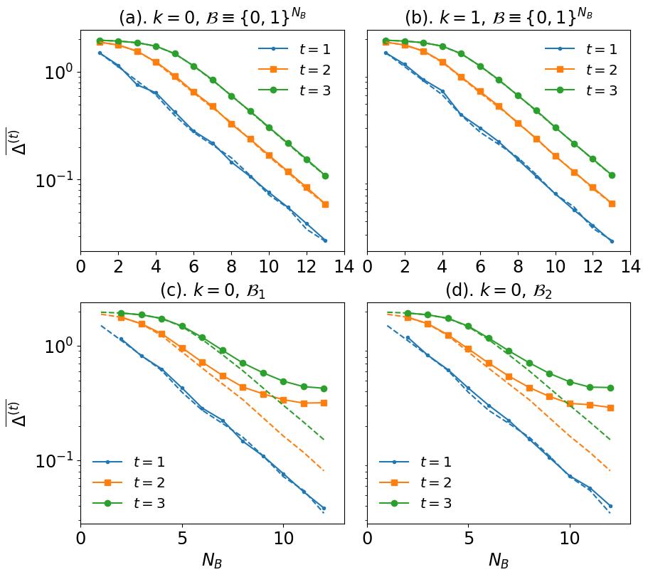
Figure 2: Illustration of $\overline{\Delta^{(t)}}$ versus $N_{B}$ for the projected ensembles of T-invariant generator states sampled uniformly at random from $\mathcal{E}^{k}_{\text{TI}}$. The results are shown for the first three moments. In the top panels (a) and (b), the measurements are performed in the computational basis: $\{\Pi_{b}=|b\rangle\langle b|$ for all $b\in\{0,1\}^{N_{B}}\}$, where $\{0,1\}^{N_{B}}$ denotes the set of all $N_{B}$-bit strings. While (a) represents the numerical computations in the $k=0$ momentum sector, $k=1$ is considered in panel (b). The results are averaged over ten initial generator states. The results appear qualitatively similar for both the momentum sectors. The trace distance falls to zero with an exponential scaling $\sim 2^{-N_{B}/2}$ for all the moments calculated. The calculations in (c) and (d) are performed in the momentum sector $k=0$ for two different measurement bases. In (c), we perform the measurements in the eigenbasis of the local translation operator supported over $B$ — $T_{B}$. In (d), we break the local translation symmetry of $T_{B}$ by applying a local Haar random unitary. We perform measurements in the eigenbasis of the resulting operator. See the main text for more details.

Figure 2 illustrates the decay of the trace distance versus $N_{B}$ for the first three moments, considering three different bases (see the description of the Fig. 2 and the next subsection) and two momentum sectors. The blue-colored curves correspond to the first moment. The blue curves, irrespective of the choice of basis and the momentum sector, always show exponential decay, i.e., $\overline{\Delta^{(1)}}\sim 2^{-N/2}$, where the overline indicates that the quantity is averaged over a few samples. We further benchmark these results against the case of Haar random generator states. For the Haar random states, the results are shown in dashed curves with the same color coding used for the first moment. We observe that the results are nearly identical in both cases, with minor fluctuations attributed to the averaging over a finite sample size.

IV.2 Higher-order state designs ($t>1$)

Here, we provide a condition for producing approximate higher-order state designs from the random T-invariant generator states.

Result IV.1.

(Sufficient condition for the identity in Eq. (12)) Given a measurement basis $\mathcal{B}$ having supported over the subsystem-$B$, then the identity in Eq. (12) holds if for all $|b\rangle\in\mathcal{B}$, $\langle b|\mathbf{T}_{k}|b\rangle=\mathbb{I}_{2^{N_{A}}}$.

The proof is given in Appendix D. For a given basis vector $|b\rangle\in\mathcal{B}$, the condition is maximally violated if it can be extended to have support over the full system such that it becomes an eigenstate (with momentum charge $k$) of the translation operator. That is, if there exists an arbitrary $|a\rangle\in\mathcal{H}^{\otimes N_{A}}$ such that $T\left(|a\rangle\otimes|b\rangle\right)=e^{-2\pi ik/N}\left(|a\rangle\otimes|b\rangle\right)$. Then, the expectation of $\mathbf{T}_{k}$ in this state becomes $\langle ab|\mathbf{T}_{k}|ab\rangle=N$, which is in maximal violation of the sufficient condition . For example, when $k=0$, the basis states $|0\rangle^{\otimes N_{B}}$ and $|1\rangle^{\otimes N_{B}}$ of the standard computational basis can be extended to $|0\rangle^{\otimes N}$ and $|1\rangle^{\otimes N}$ respectively. So, $\langle 0|^{\otimes N}\mathbf{T}_{0}|0\rangle^{\otimes N}=\langle 1|^{\otimes N}\mathbf{T}_{0}|1\rangle^{\otimes N}=N$, correspond to the maximal violation. On the other hand, most of the basis vectors of the computational basis satisfy the sufficient condition. It is also worth noting that if $|ab\rangle$ becomes a T-invariant state with a different momentum charge ($k^{\prime}\neq k$), then $\langle ab|\mathbf{T}_{k}|ab\rangle=0$.

We now calculate the trace distance $\Delta^{(t)}$ and average it over a few sample states taken from $\mathcal{E}^{k}_{\text{TI}}$. We illustrate the results in Fig. 2 for the second (orange color) and third (green color) moments by keeping $N_{A}$ and the measurement bases as before. Similar to the case of the first moment, we contrast the results with the case of Haar random generator states represented by the dashed curves. In the panels 2a and 2b corresponding to generator states with $k=0$ and $1$, projective measurements in the computational basis show an exponential decay of the average trace distance with $N_{B}$ for both the moments. Additionally, on a semilog scale, the decays for all the moments appear to align along parallel lines at sufficiently large $N_{B}$ values. From the comparison between the Figs.2a and 2b, it is evident that there are no noticeable differences when the generator states are chosen from different momentum sectors. We also consider the eigenbasis of the local translation operator $T_{B}$ for the measurements, of which a representative case for $k=0$ is shown in Fig. 2c. We observe the average trace distances deviate from the initial exponential decay and approach non-zero saturation values. In Fig. 2d, we consider the case where the translation symmetry is broken weakly by applying a single site Haar random unitary to the left of $T_{B}$, i.e., $T^{\prime}_{B}=(u\otimes\mathbb{I}_{2^{N_{B}-1}})T_{B}$. We then consider the eigenbasis of the resultant operator $T^{\prime}_{B}$ for the measurements on $B$. Surprisingly, the trace distance still saturates to a finite value for both the moments despite the broken translation symmetry. In the following subsection, we elaborate more on the interplay between the measurement bases and the sufficient condition derived in Result. IV.1.

IV.3 Overview of the bases violating the sufficient condition

From Fig. 2, it is evident that not all measurement bases furnish higher-order state designs. Here, we analyze the degree of violation of the sufficient condition by different measurement bases. Some, like the computational basis, exhibit mild violations, while others significantly deviate from the condition. Given a measurement basis $\mathcal{B}$, we quantify the average violation of the sufficient condition using the quantity $\bm{\Delta}(\mathbf{T}_{k},\mathcal{B})/2^{N_{B}}$, where

$$\bm{\Delta}(\mathbf{T}_{k},\mathcal{B})=\sum_{|b\rangle\in\mathcal{B}}\|\langle b|\mathbf{T}_{k}|b\rangle-\mathbb{I}_{2^{N_{A}}}\|_{1}.$$ (17)

In general, finding bases that fully satisfy the condition, implying $\bm{\Delta}(\mathbf{T}_{k},\mathcal{B})=0$, is hard. Depending upon $\mathcal{B}$, this quantity will display a multitude of behaviors. Also, note that for a single site unitary $u$, the local transformation of $|b\rangle$ to $|b^{\prime}\rangle=u^{\otimes N_{B}}|b\rangle$ leaves $\bm{\Delta}(\mathbf{T}_{k},\mathcal{B})$ invariant. To see the nature of the violation in a generic basis, we numerically examine $\bm{\Delta}(\mathbf{T}_{k},\mathcal{B})/2^{N_{B}}$ versus $N_{B}$ for three different bases, namely, the computational basis, a Haar random product basis, and a Haar random entangling basis, all supported over $B$.

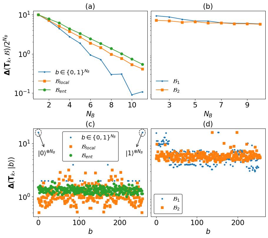
Figure 3: The figure illustrates the average violation of the sufficient condition by different bases as quantified by $\bm{\Delta}(\mathbf{T}_{k},\mathcal{B})/2^{N_{B}}$. Here, we fix $N=3$. In panel (a), $\bm{\Delta}(\mathbf{T}_{k},\mathcal{B})/2^{N_{B}}$ versus $N_{B}$ is plotted for three different bases, namely, (i) the computational basis or $\sigma^{z}$ basis (blue), (ii) basis obtained by applying local Haar random unitaries on the computational basis (orange), and (iii) an entangled basis obtained by applying a Haar unitary of dimension $2^{N_{B}}$ on the computational basis (green). For all three bases, $\bm{\Delta}(\mathbf{T}_{k},\mathcal{B})$ decays exponentially with $N_{B}$. In panel (b), the measurements are performed in the eigenbases of the operators $T_{B}$ and $u_{N_{A}+1}T_{B}$, where $T_{B}$ is the local translation operator supported over the subsystem $B$ and $u_{N_{A}+1}$ denotes a local Haar unitary acting on a site labeled with $N_{A}+1$. The violation stays nearly constant with $N_{B}$ for these two bases. In the bottom panels (c) and (d), the violation is quantified for each basis vector by fixing $N=11$. Here, we plot $\|\langle b|\mathbf{T}_{k}|b\rangle\|_{1}$ for each $|b\rangle\in\mathcal{B}$ for all the bases considered in the above panels. See the main text for more details.

The results are shown in Fig. 3. In Fig. 3a, the blue curve represents the violation for the computational basis. Clearly, the decay of the violation is exponential and faster than the other cases considered. The orange curve represents the case of local random product basis. This can be obtained by applying a tensor product of Haar random local unitaries on the computational basis vectors. As the figure depicts, the violation still decays exponentially but slower than in the case of computational basis. Finally, we consider a random entangling basis by applying global Haar unitaries on the computational basis vectors. The violation still decays exponentially but slower than the previous two. In Fig. 3c, we plot the violation for each basis vector of the above bases considered while keeping $N_{B}$ fixed. We see that, except for a few vectors, the violation stays concentrated near a value of order $O(1)$. In the computational basis, the only vectors $|0\rangle^{\otimes N_{B}}$ and $|1\rangle^{\otimes N_{B}}$ show the maximal violation, which are encircled/marked in Fig. 3c. We consider the violation is significant if $\bm{\Delta}(\mathbf{T}_{k},\mathcal{B})/2^{N_{B}}$ does not decay with $N_{B}$. If this happens, the projected ensembles may fail to converge to the state designs even in the large $N_{B}$ limit. Note that, while the exponential decay of the violation may appear generic, there exist bases that show nearly constant violation as $N_{B}$ increases, which are depicted in Fig. 2b and 2d.

To explore such measurement bases with significant violations, we consider the following.

$$\bm{\Delta}(\mathbf{T}_{k},\mathcal{B}) =\sum_{|b\rangle\in\mathcal{B}}\left\|\langle b|\sum_{j=0}^{N-1}e^{2\pi ijk/N}T^{j}|b\rangle-\mathbb{I}_{2^{N_{A}}}\right\|_{1}$$

$$=\sum_{|b\rangle\in\mathcal{B}}\left\|\sum_{j=1}^{N-1}e^{2\pi ijk/N}\langle b|T^{j}|b\rangle\right\|_{1}$$

$$=\sum_{|b\rangle\in\mathcal{B}}\left(\left\|e^{2\pi ir/N}\langle b|T^{r}|b\rangle+\sum_{j\neq r}e^{2\pi ijk/N}\langle b|T^{j}|b\rangle\right\|_{1}\right).$$ (18)

In the second line, we used the fact $\langle b|\mathbb{I}_{2^{N}}|b\rangle=\mathbb{I}_{2^{N_{A}}}$ and subtracted it from $e^{2\pi i0/N}\langle b|T^{0}|b\rangle$. In the third equality, a term corresponding to an arbitrary integer $r$ in the summation, where $1\leq r\leq N-1$, has been isolated from the remaining terms. This enables the analysis of violations with respect to each element of the translation group, facilitating the identification of the violating bases. To illustrate this, we consider the specific case where $r=1$:

$$\langle b|T|b\rangle = \langle b|S_{1,2}S_{2,3}\cdots S_{N-1,N}|b\rangle$$ (19)

$$= \left(S_{1,2}\cdots S_{N_{A}-1,N_{A}}\right)\langle b|S_{N_{A},N_{A}+1}\cdots S_{N-1,N}|b\rangle$$

$$= \int_{u}d\mu(u)\left(T_{A}u^{\dagger}_{N_{A}}\right)\langle b|u_{N_{A}+1}T_{B}|b\rangle,$$

where $S_{i,i+1}$ denotes the swap operator between $i$ and $i+1$ sites, $T_{A}$ and $T_{B}$ are translation operators locally supported over the subsystems $A$ and $B$. In the third equality, $S_{N_{A},N_{A}+1}$ is replaced by the unitary Haar integral expression of the swap operator — $S_{N_{A},N_{A}+1}=\int_{u}d\mu(u)(u^{\dagger}_{N_{A}}\otimes u_{N_{A}+1})$, where $d\mu(u)$ represents the invariant Haar measure over the unitary group $U(2)$ Zhang (2014). Then, we heuristically argue that the measurements in the eigenbasis of the operator $u_{N_{A}+1}T_{B}$ for an arbitrary $u$ would lead to $\bm{\Delta}(\mathbf{T}_{k},\mathcal{B})\sim O(2^{N})$. Consequently, the average violation $\bm{\Delta}(\mathbf{T}_{k},\mathcal{B})/2^{N_{B}}$ stays nearly a constant of order $O(2^{N_{A}})$ even in the large $N_{B}$ limit. We illustrate this by considering the eigenbases of the operator $u_{N_{A}+1}T_{B}$ in Fig. 3b and 3d for two cases of $u_{N_{B}}$, namely, $u_{N_{B}}=\mathbb{I}_{2}$ and a Haar random $u_{N_{B}}$. Infact, we considered the same measurement bases in Figs. 2c and 2d and observed that the projected ensembles do not converge to the higher-order state designs. It is interesting to notice that the measurement bases that do not respect the translation symmetry can also hinder the design formation [see Fig. 2d]. In Appendix E, we elaborate this aspect further by considering $r=2$ in Eq. (IV.3).

V Deep thermalization in a chaotic Hamiltonian

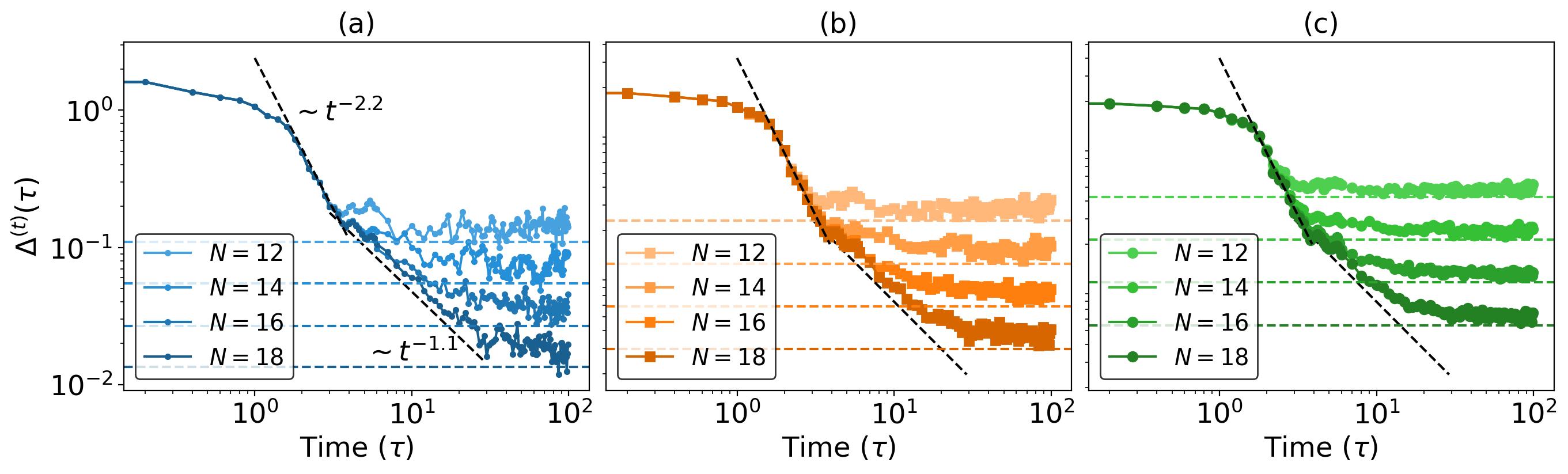
Figure 4: Deep thermalization or dynamical generation of state designs (as characterized by $\Delta^{(t)}(\tau)$) of a quantum state $|\psi(\tau)\rangle$ evolved under the dynamics of a chaotic Ising Hamiltonian with periodic boundary conditions. Here, the evolution time is denoted with $\tau$, and the initial state is taken to be $|0\rangle^{\otimes N}$. The results are shown for the first three moments ($t=1,2$, and $3$) in the sequential order along the row. The size of the projected ensembles $N_{A}$ is fixed at $3$. For each moment, the numerics are carried out for different system sizes varying from $N=12$ to $N=18$. Note the color coding: The darker colors indicate larger system sizes, and the lighter colors denote smaller system sizes. The dashed lines in all the panels with varying intensities represent the value attained by the typical random T-invariant states sampled from $\mathcal{E}^{k}_{\text{TI}}$, where $k=0$. From the numerical results, we observe a two-step relaxation of $\Delta^{(t)}(\tau)$ towards the saturation. See the main text for more details.

In the preceding section, our analysis focused on obtaining state designs from random T-invariant states. Here, we examine the dynamical generation of the state designs in a tilted field Ising chain with periodic boundary conditions (PBCs). The corresponding Hamiltonian is given by

$$H=\sum_{i=0}^{N}\sigma^{x}_{i}\sigma^{x}_{i+1}+h_{x}\sum_{i=0}^{N}\sigma^{x}_{i}+h_{y}\sum_{i=0}^{N}\sigma^{y}_{i},$$ (20)

where the PBCs correspond to $\sigma^{x,y,z}_{N+i}=\sigma^{x,y,z}_{i}$. The periodicity, along with the homogeneity of the interactions and the magnetic fields, makes the system translation invariant, i.e., $[H,T]=0$. In addition, the Hamiltonian is reflection invariant about every site. For the parameters $h_{x}=(\sqrt{5}+1)/4$ and $h_{y}=(\sqrt{5}+5)/8$, the system is chaotic, and the ETH has been thoroughly verified in Ref. Kim et al. (2014). Furthermore, deep thermalization has also been investigated in this model with open boundary conditions (OBCs) in Ref. Cotler et al. (2023) and Bhore et al. (2023). Here, we explore this aspect for the Hamiltonian in Eq. (20) and contrast the results with those of OBCs. To proceed, we consider a trivial product state $|\psi\rangle=|0\rangle^{\otimes N}$ as the initial state and evolve it under the Hamiltonian. The initial state is an eigenstate of $T$ with the eigenvalue $1$, i.e., $T|0\rangle^{\otimes N}=|0\rangle^{\otimes N}$. Since the Hamiltonian also commutes with $T$, the final state $|\psi(\tau)\rangle=e^{-i\tau H}|0\rangle^{\otimes N}$ will remain T-invariant with the same eigenvalue, where $\tau$ denotes the time of evolution. As this state evolves, we construct and examine its projected ensembles at different times. The computational basis is considered for the projective measurements on $B$. The corresponding numerical results are shown in Fig. 4.

Figures 4a-4c demonstrate the decay of $\Delta^{(t)}$ as a function of evolution time ($\tau$) for the first three moments, $t=1$, $2$, and $3$, respectively. We show this evolution for different system size $N$ by considering $N_{A}=3$ fixed and changing $N_{B}$. The evolution of $\Delta^{(t)}(\tau)$ suggests a two-step relaxation towards the saturation. Initially, over a short period, the trace distance $\Delta^{(t)}(\tau)$ scales like $\sim t^{-2.2}$ for all three moments. For the largest considered system size, $N=18$, this power law behavior spans across the region $1\lesssim\tau\lesssim 4$. Moreover, this time scale appears to grow with $N_{B}$, which can be read off from the plots. Note that in Ref. Cotler et al. (2023), the initial decay has been observed to be $\sim t^{-1.2}$ for the model with OBC [see Appendix F]. In contrast, the present case exhibits a nearly doubled exponent of the power law behavior. Interestingly, similar behavior characterized by exponential decay has been observed in Ref. Shrotriya and Ho (2023), where the authors focused on dual unitary circuits and contrasted the case of PBCs with OBCs. The doubled exponent for the PBCs in our case can be attributed to the periodicity of the Hamiltonian since the entanglement across the bi-partition $AB$ grows at a rate twice the rate in the case of OBC Mishra et al. (2015); Pal and Lakshminarayan (2018). To elucidate the role of entanglement growth at initial times, we examine the trace distance for the simplest case $t=1$, i.e., $\Delta^{(1)}(\tau)$. Since the first moment of the projected ensemble is simply the reduced density matrix of $A$, the trace distance can be written as

$$\Delta^{(1)}(\tau)=\left\|\rho_{A}(\tau)-\dfrac{\mathbb{I}}{2^{N_{A}}}\right\|_{1}=\sum_{j=0}^{2^{N_{A}}-1}\left|\gamma^{2}_{j}(\tau)-\dfrac{1}{2^{N_{A}}}\right|,$$ (21)

where $\rho_{A}(t)=\Tr_{B}(|\psi(t)\rangle\langle\psi(t)|)$ and $\{\gamma_{j}\}$ denote the Schmidt coefficients of $|\psi(t)\rangle$ across the bipartition. Above expression relates $\Delta^{(1)}(\tau)$ to the fluctuations of the Schmidt coefficients around $1/2^{N_{A}}$, corresponding to the maximally mixed value. At the time $\tau=0$, as the considered initial state is a product state, the only non-zero Schmidt coefficient is $\gamma_{0}(\tau=0)=1$. Hence, it is fair to say that $\Delta^{(1)}(0)$ is largely dominated by the decay of $\gamma_{0}$ during the early times. This regime usually witnesses inter-subsystem scrambling of the initial state mediated by the entanglement growth. Moreover, the initial decay appears across all three panels with the same power law scaling, indicating a similar early-time dependence of $\Delta^{t}(\tau)$ over $\gamma_{0}(\tau)$.

Beyond the initial power-law regime, we observe a crossover to an intermediate-time power-law decay regime with a smaller exponent, which is followed by saturation at a large time. In the intermediate decay regime, the power-law exponent depends on the system size $N$, yielding a non-universal characteristic. For $N=18$, we obtain $\Delta^{(t)}\sim t^{-1.1}$, which is to be contrasted with the early-time decay exponent. At the onset of this scaling, the largest Schmidt coefficient $\gamma_{0}$ becomes comparable with the other $\gamma_{j}$s. The corresponding timescale is referred to as collision time Žnidarič et al. (2012). At the collision time, $\gamma_{0}$ comes close to $\gamma_{1}$, the second largest Schmidt-coefficient. Hence, $\gamma_{0}$ does not solely determine the decay of $\Delta^{(1)}(\tau)$. The two-step relaxation of quantum systems has been recently studied in systems with two or more symmetries and also in quantum circuit models Bensa and Žnidarič (2022); Žnidarič (2023). Finally, we benchmark the late time saturation values for each $N$ using the random matrix theory (RMT) predictions for the T-invariant ensembles. We do this by plotting horizontal (dashed) lines corresponding to the RMT values. We notice that the saturation for the model happens slightly above the corresponding RMT predictions. This could be due to the presence of reflection symmetries, yet they do not seem to play any significant role in constraining the early and intermediate time decay behaviors. The saturation trend can be contrasted with the case having OBCs, where it is known to happen exactly at RMT predicted values Cotler et al. (2023). We intuitively expect the two-step relaxation observed in the case of PBCs to arise from its two competing features: initial faster decay and late time saturation above random matrix prediction.

VI Generalization to other symmetries

In the preceding sections, we examined the emergence of state designs from the translation symmetric generator states. In this section, we extend these findings to other symmetries, specifically considering $Z_{2}$ and reflection symmetries as representative examples.

VI.1 $Z_{2}$-symmetry

The group associated with $Z_{2}$-symmetry consists of two elements $\{\mathbb{I}_{2^{N}},\Sigma\}$, where $\Sigma=\otimes_{i=1}^{N}\sigma^{x}_{i}$. If a system is $Z_{2}$-symmetric, its Hamiltonian will be invariant under the action of $\Sigma$, i.e., $\Sigma H\Sigma=H$. On the other hand, a quantum state $|\psi\rangle$ is considered $Z_{2}$-symmetric if it is an eigenstate of the operator $\Sigma$ with an eigenvalue $\pm 1$. Here, similar to the case of translation symmetry, we first construct an ensemble of $Z_{2}$-symmetric states by projecting the Haar random states onto a $Z_{2}$-symmetric subspace. We then follow the analysis of state designs using the projected ensemble framework.

Given a Haar random state $|\psi\rangle\in\mathcal{E}_{\text{Haar}}$ that has support over $N$-sites, then

$$|\psi\rangle\rightarrow|\phi\rangle=\dfrac{1}{\mathcal{N}}\mathbf{Z}_{k}|\psi\rangle$$ (22)

is a $Z_{2}$-symmetric state with an eigenvalue $(-1)^{k}$ with $k\in\{0,1\}$, where $\mathbf{Z}_{k}=\mathbb{I}+(-1)^{k}\Sigma\quad\text{and }\mathcal{N}=\sqrt{\langle\psi|\mathbf{Z}^{\dagger}_{k}\mathbf{Z}_{k}|\psi\rangle}=\sqrt{2\langle\psi|\mathbf{Z}_{k}|\psi\rangle}$. Introducing this symmetry reduces the randomness of the Haar random state by a factor of $2$. Specifically, the number of independent complex parameters needed to describe the state scales like $\sim O(2^{N-1})$. Using similar techniques employed for the T-invariant states, the moments of $Z_{2}$-symmetric ensembles can be evaluated as

$$\mathbb{E}_{\phi\in\mathcal{E}^{k}_{Z_{2}}}\left[\left[|\phi\rangle\langle\phi|\right]^{\otimes t}\right]=\dfrac{\mathbf{Z}^{\otimes t}_{k}\bm{\Pi}_{t}}{\Tr\left(\mathbf{Z}^{\otimes t}_{k}\bm{\Pi}_{t}\right)}.$$ (23)

To analyze the projected ensembles, we first fix the measurements on $N_{B}$ sites in the computational basis, i.e., $\{|b\rangle\langle b|\}$ for all $|b\rangle\in\{0,1\}^{N_{B}}$. To get approximate state designs, it is sufficient to have $\langle b|\mathbf{Z}_{k}|b\rangle\approx\mathbb{I}_{2^{N_{A}}}$ for a sufficiently large number of $b\in\{0,1\}^{N_{B}}$. In the case of $Z_{2}$-symmetry, this is indeed satisfied as we have $\langle b|\mathbf{Z}_{k}|b\rangle=\mathbb{I}_{2^{N_{A}}}+(-1)^{k}\langle b|\Sigma|b\rangle$, where the second term can be simplified as

$$\langle b|\Sigma|b\rangle=\left(\otimes_{j=1}^{N_{A}}\sigma^{x}_{j}\right)\left(\langle b_{1}|\sigma^{x}|b_{1}\rangle...\langle b_{N_{B}}|\sigma^{x}|b_{N_{B}}\rangle\right).$$ (24)

The terms within the brackets are the diagonal elements of $\sigma^{x}$ operator, which are zeros in the computational basis, implying that $\langle b|\Sigma|b\rangle=0$. Therefore, in this case, the sufficient condition is exactly satisfied. Consequently, the projected ensembles converge to the state designs for large $N_{B}$. The numerical results for the average trace distance are shown in Fig. 5. We notice that the results nearly coincide with the case of Haar random generator states [see Fig. 5a and 5b].

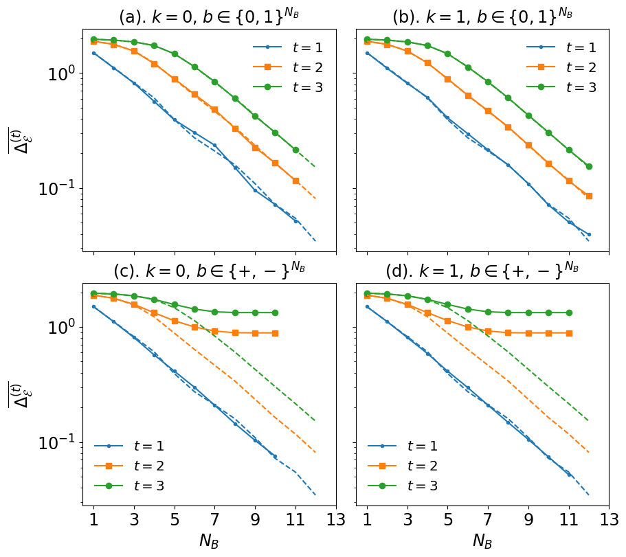
Figure 5: Average trace distance ($\overline{\Delta^{(t)}}$) between the moments of the projected ensembles and the moments of the Haar random states supported over $N_{A}$ sites, plotted against $N_{B}$. The initial states are chosen uniformly at random from the ensemble of $Z_{2}$-symmetric quantum states. The average is computed over a ten samples of the initial generator states. In (a) and (b), the measurements are performed in the computational ($\sigma^{z}$) basis — $\{|b\rangle\langle b|\}$ for all $b\in\{0,1\}^{N_{B}}$. While the states chosen in (a) have the eigenvalue $1$, the other panel is plotted for the states with eigenvalue $-1$. We repeat the same calculation in the panels (c) and (d) with the measurement basis given by $\{|b\rangle\langle b|\}$ for all $b\in\{+,-\}^{N_{B}}$, where $|+\rangle$ and $|-\rangle$ represent the eigenstates of $\sigma^{x}$ and are connected to $|0\rangle$ and $|1\rangle$ through the Hadamard transform.

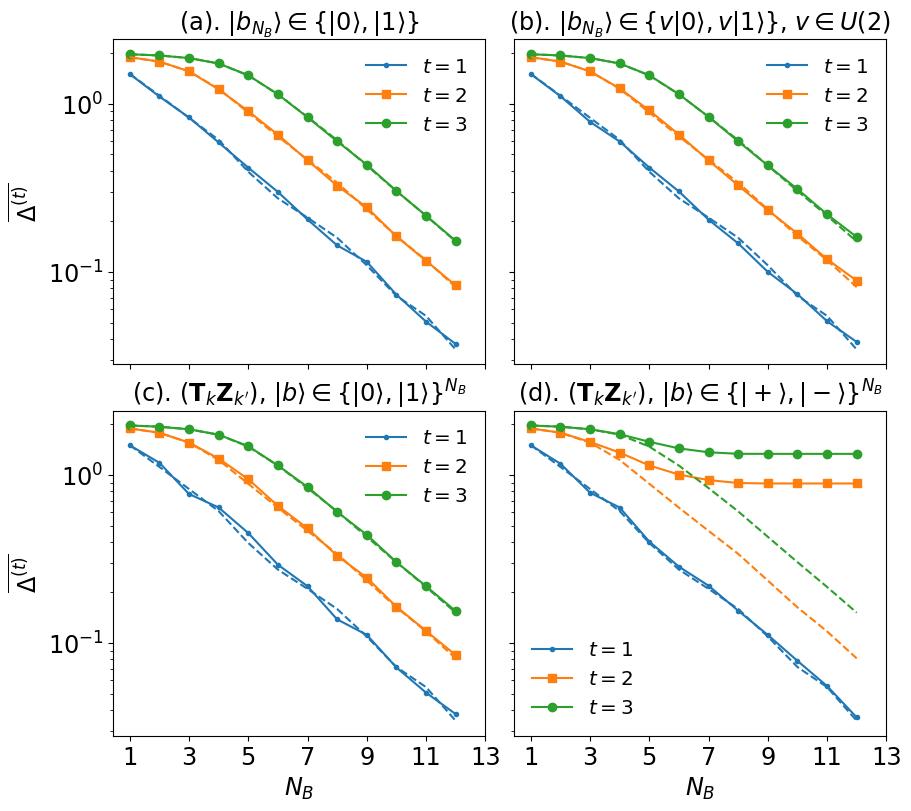
Figure 6: The figure illustrates $\overline{\Delta^{(t)}}$ versus $N_{B}$. In (a), the measurements are performed in the eigenbasis of the operator $\sigma^{x}\otimes\cdots\otimes\sigma^{x}\otimes\sigma^{z}$, where the tensor product of $\sigma^{x}$ operators have support over $N_{B}-1$ sites and $\sigma^{z}$ is supported over $N_{B}$-th site. In (b), we replace the eigenbasis of $\sigma^{z}$ on $N_{B}$-th site with an eigenbasis of single site Haar random unitary. Here, we fix the charge $k=0$. In (c) and (d), we take the random generator states that are simultaneous eigenstates of both $T$ and $\Sigma$. While the measurement basis in $c$ is the computational basis, the eigenbasis of $\sigma^{x}$ is considered for measurements in (d). Here, the charges are fixed at $k=k^{\prime}=0$.

However, if the measurements are performed in $\sigma^{x}$ basis, given by $\{|b\rangle\langle b|\}$ for all $b\in\{+,-\}^{N_{B}}$, where $|+\rangle=(|0\rangle+|1\rangle)/\sqrt{2}$ and $|-\rangle=(|0\rangle-|1\rangle)/\sqrt{2}$, then $\langle\pm|\sigma^{x}|\pm\rangle=\pm 1$. As a result, the projected ensembles deviate significantly from the quantum state designs. The violation from the sufficient condition in this case, as quantified by $\bm{\Delta}(\mathbf{Z}_{k},\mathcal{B})/2^{N_{B}}$, remains a constant for any $N_{B}$:

$$\dfrac{\bm{\Delta}(\mathbf{Z}_{k},\mathcal{B})}{2^{N_{B}}} =\dfrac{1}{2^{N_{B}}}\sum_{b\in\{+,-\}^{N_{B}}}\left\|\langle b|\mathbf{Z}_{k}|b\rangle-\mathbb{I}_{2^{N_{A}}}\right\|_{1}$$

$$=\dfrac{1}{2^{N_{B}}}\sum_{b\in\{+,-\}^{N_{B}}}\left\|(-1)^{k+\sum_{i=1}^{N_{B}}\text{sgn}(b_{i})}\otimes_{j=1}^{N_{A}}\sigma^{x}_{j}\right\|$$

$$=2^{N_{A}}.$$ (25)

We demonstrate the numerical results of the average distance in Figs. 5c and 5d. In contrast to the computational basis measurements, here, only the first moment coincides with the case of Haar random generator states, while the higher moments appear to saturate to a finite value of $\overline{\Delta^{(t)}}$.

We now consider a case where we perform the local measurements on $N_{B}$-th site in $\sigma^{z}$ basis while keeping $\sigma^{x}$ measurement basis for the remaining $N_{B}-1$ sites. We represent the resultant basis with $b^{\prime}\in\{+,1\}^{N-1}\times\{0,1\}$. Then,

$$\langle b^{\prime}|\mathbf{Z}_{k}|b^{\prime}\rangle=\mathbb{I}_{2^{N_{A}}}+(-1)^{k}\langle b^{\prime}|\Sigma|b^{\prime}\rangle,$$ (26)

where the second term vanishes as $\langle b^{\prime}_{N_{B}}|\sigma^{x}_{N_{B}}|b^{\prime}_{N_{B}}\rangle=0$. Therefore, we have $\langle b^{\prime}|\Sigma|b^{\prime}\rangle=0$ for all $|b^{\prime}\rangle$, implying the required condition for the convergence of quantum state designs. The corresponding results for the average trace distances are shown in Fig. 6a. In Fig. 6b, we replace the $\sigma^{x}$ basis on $N_{B}$-th site with a local Haar random basis. We find no significant differences between 6a and 6b within the range of $N_{B}$ considered for the numerical simulations. This demonstrates that a mild modification of the measurement basis can retrieve the state design if the sufficient condition is satisfied. So, the sufficient condition allows us to infer suitable measurement bases for obtaining higher-order state designs, which might not be apparent otherwise.

For completeness, we also demonstrate the emergence of state designs from the generator states that respect both translation and $Z_{2}$-symmetry. Since $T$ and $\Sigma$ commute, one can easily construct the states that respect both the symmetries by applying corresponding projectors consecutively on an initial state. Let $|\psi\rangle$ denote a Haar random state, then $|\phi\rangle=\mathbf{T}_{k_{1}}\mathbf{Z}_{k_{2}}|\psi\rangle/\sqrt{\mathcal{N}}$, where $\mathcal{N}=\sqrt{2N\left(\mathbf{T}_{k_{1}}\mathbf{Z}_{k_{2}}\right)}$, is a random vector that is simultaneously an eigenvector of both $T$ and $\Sigma$ with respective charges $k_{1}$ and $k_{2}$. Then, the condition to get quantum state designs from the projected ensembles would be $\langle b|\mathbf{T}_{k_{1}}\mathbf{Z}_{k_{2}}|b\rangle=0$ for all $|b\rangle\in\mathcal{B}$. The projective measurements in the standard computational basis mildly violate this condition, which results in the convergence towards state designs. The numerical results are shown in 6c and 6d. While the former is plotted by taking the computational basis measurements, the latter represents the results for the local measurements in $\sigma^{x}$ basis, i.e., $b\in\{+,-\}^{N_{B}}$.

VI.2 Reflection symmetry

Here, we employ the projected ensemble framework for the generator states having reflection or mirror symmetry. In a system exhibiting reflection symmetry, the Hamiltonian remains invariant under swapping of mirrored sites around the center. Let $R$ denote the reflection operation. Then $R$ generates a cyclic group of two elements, namely, the identity $\mathbb{I}$ and $R$ itself. In an $N$-qubit system, $R$ is defined as

$$R=\begin{cases}S_{1,N}S_{2,N-1}....S_{N/2,N/2+1}&\quad\textrm{if }N\textrm{ is even}\\ S_{1,N}S_{2,N-1}....S_{(N-1)/2,(N+3)/2}&\quad\textrm{if }N\textrm{ is odd.}\end{cases}$$ (27)

The reflection operator has $\{-1,1\}$ as its eigenvalues. Hence, the total Hilbert space admits a decomposition into two invariant sectors. Then, the Hermitian operators $\mathbf{R}_{\pm}=\mathbb{I}\pm R$ project arbitrary states onto the respective subspaces. Engineering state designs from these generator states would require $\langle b|\mathbf{R}_{\pm}|b\rangle=\mathbb{I}_{2^{N_{A}}}$ for all $|b\rangle\in\mathcal{B}$.

We consider a product basis $\mathcal{B}\equiv\{u|0\rangle,u|1\rangle\}^{\otimes N_{B}}$ for the measurements, where $u$ is an arbitrary unitary operator. For some $|b\rangle\in\mathcal{B}$, we have $\langle b|\mathbf{R}_{\pm}|b\rangle=\mathbb{I}_{2^{N_{A}}}\pm\langle b|R|b\rangle$. Since $\mathcal{B}$ is assumed to be a local product basis, we can write $|b\rangle=|b_{N_{A}+1}b_{N_{A}+2}...b_{N}\rangle$. To be explicit in calculating $\langle b|R|b\rangle$, let us consider $N_{A}=3$ and $N_{B}=N-3\geq N_{A}$. Then,

$$\langle b|R|b\rangle=$$

$$\underbrace{|b_{N}b_{N-1}b_{N-2}\rangle\langle b_{N}b_{N-1}b_{N-2}|}_{\text{Supported on }A}\underbrace{\delta_{b_{4},b_{N-3}}\delta_{b_{5},b_{N-4}}...\delta_{b_{(N-1)/2},b_{(N+3)/2}}}_{\text{palindrome condition}}.$$ (28)

Thus, $\langle b|R|b\rangle$ remains a non-zero operator only when the palindrome condition on the first $N_{B}-N_{A}$ bits of the string-$b$ is satisfied. If $N_{B}-N_{A}$ is even (odd), then we have a total of $n_{\text{even}}=2^{(N_{B}-N_{A})/2}$ ($n_{\text{odd}}=2^{(N_{B}-N_{A}+1)/2}$) distinct palindromes. Then, the total number of violations of the condition for the given measurement basis will be $n_{\text{even}(\text{odd})}2^{N_{A}}$. For even-$N$, this number is exactly $2^{N/2}$. Moreover, the violation of the sufficient condition in the considered basis is

$$\dfrac{\bm{\Delta}(\mathbf{R}_{k},\mathcal{B})}{2^{N_{B}}} = \dfrac{1}{2^{N_{B}}}\sum_{|b\rangle\in\mathcal{B}}\|\langle b|R|b\rangle\|_{1}$$ (29)

$$= \begin{cases}2^{-N/2},&\text{if }N\text{ is even}\\ 2^{-(N-1)/2},&\text{otherwise.}\end{cases}$$

Since $\bm{\Delta}(\mathbf{R}_{k},\mathcal{B})/2^{N_{B}}$ is exponentially suppressed as $N$ increases, the moments of the projected ensembles converge to the Haar moments. We plot the average $\Delta^{(t)}$ versus $N_{B}$ in Fig. 7. To illustrate, we consider the computational basis and random entangling basis for the measurement in 7a and 7b, respectively. The later basis states can be obtained by the application of a fixed Haar random unitary supported over $B$ on the computational basis vectors. The results in both panels coincide with the case of Haar random generator states, implying the generation of higher-order state designs.

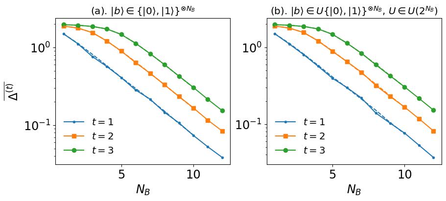
Figure 7: Illustration of $\overline{\Delta^{(t)}}$ vs $N_{B}$ for the random generator states with the reflection symmetry for the first three moments. We fix the charge $k=0$. In (a), the computational basis measurements are considered. In (b), the measurements are performed in a random product basis. We find no noticeable differences between these two. Moreover, the decay nearly coincides with the case when the generator states are Haar random.

VII Summary and Discussion

In summary, we have investigated the role of symmetries on the choice of measurement basis for quantum state designs within the projected ensemble framework. By employing the tools from Lie groups and measure theory, we have evaluated the higher-order moments of the symmetry-restricted ensembles. Using these, we have derived a sufficient condition on the measurement basis for the emergence of higher-order state designs. The condition reads as follows: Given an arbitrary measurement basis $\mathcal{B}\equiv\{|b\rangle\}$ over a subsystem-$B$, for a typical $Q$-symmetric state $|\psi_{AB}\rangle\in\mathcal{E}^{k}_{\text{Q}}$ with a charge $k$, $\langle b|\mathbf{Q}_{k}|b\rangle=\mathbb{I}_{2^{N_{A}}}$ for all $|b\rangle\in\mathcal{B}$ implies that the projected ensembles approximate higher-order state designs. Moreover, the approximation improves exponentially with $N_{B}$, the bath size. While the condition is sufficient for the emergence of state designs, the necessity of it remains an open question. We demonstrate its versatility by considering measurement bases violating the condition mildly. Our analysis further suggests that a significant violation of the condition likely prevents the convergence of projected ensembles to the designs even in the limit of large $N_{B}$. To elucidate it, we have quantified the extent to which a basis violates the sufficient condition using the quantity $\sum_{|b\rangle\in\mathcal{B}}\|\langle b|\mathbf{Q}_{k}|b\rangle-\mathbb{I}_{2^{N_{A}}}\|_{1}/2^{N_{B}}$. This quantity allows us to identify the bases that violate the condition significantly. We have shown that the measurements in these bases result in a finite value for the trace distance $\Delta^{(t)}$ even when $N_{B}$ is large. Surprisingly, these include bases that do not adhere to the symmetry in the generator states.

To begin with, we have chosen random T-invariant states as the generator states. In constructing these states, we projected the Haar random states onto the momentum-conserving subspaces to reconcile both randomness and symmetry. This allows one to construct distinct ensembles of T-invariant states, each with a different momentum. Thanks to the inherent Haar measure in these ensembles, the states in them are uniformly distributed. Given a suitable measurement basis, Levy’s lemma then ensures that the projected ensemble of a typical T-invariant state well approximates a state design. Equipped with this argument, we have numerically verified the emergence of designs for different measurement bases. These bases include the standard computational ($\sigma^{z}$) basis and the eigenbasis of $T_{B}$. While the former nearly satisfies the sufficient condition, the latter violates it significantly. Accordingly, the trace distance $\Delta^{(t)}$ decays exponentially with $N_{B}$ for the computational basis. Whereas, for the eigenbasis of $T_{B}$, $\Delta^{(t)}$ converges to a non-zero value. To further contextualize our results in a more physical setting, we have focused on deep thermalization in a tilted field Ising chain with PBCs, respecting the translation symmetry. The results indicate that the decay of the trace distance with time occurs in two steps. The initial decay is observed to be twice the rate of the case of the same model with OBCs. In the intermediate time, the decay trend is a system-dependent power law. Whereas, in a long time, the trace distance saturates to a value slightly larger than RMT prediction, a reminiscence of other symmetries.

Due to the generality of our formalism, the results can be extended to other discrete symmetries, and are expected to hold for continuous symmetries. In particular, generalization to other cyclic groups is straightforward. To illustrate this, we have examined the projected ensembles from the generator states with $Z_{2}$ and reflection symmetries. A crucial implication of our results is that the sufficient condition plays a pivotal role in identifying appropriate measurement bases, even when their suitability is not immediately apparent.

If one considers two or more non-commuting symmetries, they do not share common eigenstates. In such systems, the equilibrium states have been shown to approximate non-abelian thermal states Majidy et al. (2023); Yunger Halpern et al. (2016). These states have been experimentally realized recently in Ref. Kranzl et al. (2023). Hence, an extensive study of deep thermalization and emergent state designs in these systems is a topic of our immediate future investigation. Additionally, measurement-induced phase transitions (MIPTs) occur due to an interplay between the measurements and the dynamics in many-body chaotic systems Skinner et al. (2019). Our results can offer insights into the mechanism of the MIPTs whenever the dynamics and the measurements are chosen to respect symmetries.

Appendix A Details on the construction of random T-invariant unitaries

The QR decomposition is traditionally used to generate Haar random unitary operators from the initial random Gaussian matrices. However, QR decomposition can not produce uniformly distributed unitaries from the subgroups such as $U_{\text{TI}}(d^{N})$ as the decomposition does not preserve the symmetries of the initial operator. Here, we use polar decomposition as an alternative to the QR decomposition to generate random unitary operators. For a given initial operator $Z$, the polar decomposition is given by $Z=UP$, where $P$ is a positive semi-definite operator, $P=\sqrt{Z^{\dagger}Z}$. If $Z$ is a full rank matrix, $U=Z(Z^{\dagger}Z)^{-1/2}$ can be uniquely computed. If $Z$ is a complex Gaussian matrix with mean $\mu=0$ and standard deviation $\sigma=1$, the polar decomposition will yield the ensemble of unitaries whose moments match those of the Haar random unitaries. To see this, consider $A$, an arbitrary operator acting on $t$-replicas of the same Hilbert space $\mathcal{H}^{d}$. Then, we have

$$\langle U^{\dagger\otimes t}AU^{\otimes t}\rangle = \int_{Z}d\mu(Z)\left(Z(Z^{\dagger}Z)^{-1/2}\right)^{\dagger\otimes t}A\left(Z(Z^{\dagger}Z)^{-1/2}\right)^{\otimes t}$$ (30)

$$= \int_{Z}d\mu(Z)\left((Z^{\dagger}Z)^{-1/2}Z^{\dagger}\right)^{\otimes t}A\left(Z(Z^{\dagger}Z)^{-1/2}\right)^{\otimes t},$$

where $d\mu(Z)$ denotes the invariant measure over the Ginebre ensemble. Since the Ginibre ensemble is unitarily invariant, we replace $Z$ with $VZ$ for some $V\in U(d^{N})$ and perform Haar integral over $V$. This action keeps the overall integral in the above equation invariant.

$$\langle U^{\dagger\otimes t}AU^{\otimes t}\rangle = \int_{Z}d\mu(Z)\int_{V\in U(d^{N})}d\mu(V)\left((Z^{\dagger}Z)^{-1/2}Z^{\dagger}V^{\dagger}\right)^{\otimes t}A\left(VZ(Z^{\dagger}Z)^{-1/2}\right)^{\otimes t}$$ (31)

$$= \int_{Z}d\mu(Z)\left((Z^{\dagger}Z)^{-1/2}Z^{\dagger}\right)^{\otimes t}\left(\int_{V\in U(d^{N})}d\mu(V)V^{\dagger\otimes t}AV^{\otimes t}\right)\left(Z(Z^{\dagger}Z)^{-1/2}\right)^{\otimes t}.$$

By the Schur-Weyl duality, $\int_{V\in U(d^{N})}d\mu(V)V^{\dagger\otimes t}AV^{\otimes t}=\sum_{i=1}^{t!}c_{i}\pi_{i}$, where $\{\pi_{i}\}$s are permutation operators acting on $t$-replicas of the Hilbert space. It then follows that

$$\langle U^{\dagger\otimes t}AU^{\otimes t}\rangle=\left(\int_{V\in U(d^{N})}d\mu(V)V^{\dagger\otimes t}AV^{\otimes t}\right)\left(\int_{Z}d\mu(Z)\left((Z^{\dagger}Z)^{-1/2}Z^{\dagger}\right)^{\otimes t}\left(Z(Z^{\dagger}Z)^{-1/2}\right)^{\otimes t}\right).$$ (32)

Since $Z(Z^{\dagger}Z)^{-1/2}=U$ is a unitary operator, the integrand of the second integral becomes the Identity operator. Therefore,

$$\langle U^{\dagger\otimes t}AU^{\otimes t}\rangle=\int_{V\in U(d^{N})}d\mu(V)V^{\dagger\otimes t}AV^{\otimes t}.$$ (33)

This equation implies that the moments of the ensemble of unitaries from the polar decomposition are identical to those of the Haar ensemble of unitaries.

We now show that if the initial operator commutes with an arbitrary unitary operator, then the resulting unitary from the polar decomposition necessarily commutes with the same. For our purpose, we take the commuting unitary to be $T$, the translation operator. Let $Z$ be randomly drawn from the Ginibre ensemble. Then, the operator $Z^{\prime}=\sum_{j=0}^{N-1}T^{\dagger j}ZT^{j}$ is translation invariant as $T^{\dagger}Z^{\prime}T=Z^{\prime}$. Moreover, $P^{\prime}=\sqrt{Z^{{}^{\prime}\dagger}Z^{\prime}}$ is also $T$-invariant whenever $Z^{\prime}$ is a full rank matrix. Consequently, the resulting unitary $U^{\prime}$ commutes with $T$. One can also show that the distribution of $Z^{\prime}$ is invariant under the action of elements of $U_{\text{TI}}(d^{N})$. Therefore, the resulting ensemble of unitaries has the same moments as those of the unitary subgroup $U_{\text{TI}}(d^{N})$.

Appendix B Proof of Result III.2

Proof.

We first note that given a Haar random pure state $|\psi\rangle$, under the map $\mathbb{T}_{k}$, becomes an eigenstate of $T$ with the eigenvalue $e^{-2\pi ik/N}$, i.e., $|\phi\rangle=\mathbf{T}_{k}|\psi\rangle/\sqrt{\langle\psi|\mathbf{T}^{\dagger}_{k}\mathbf{T}_{k}|\psi\rangle}$. This generates an ensemble $\{|\phi\rangle\}$, denoted with $\mathcal{E}^{k}_{\text{TI}}$, when $|\psi\rangle\in\mathcal{E}_{\text{Haar}}$. We are interested in finding the moments associated with $\mathcal{E}^{k}_{\text{TI}}$. For any $k$, the $t$-th moment can be evaluated as follows:

$$\mathbb{E}_{\phi\in\mathcal{E}^{k}}\left[\left[|\phi\rangle\langle\phi|\right]^{\otimes t}\right]=\int_{\psi\in\mathcal{E}_{\text{Haar}}}d\psi\dfrac{\mathbf{T}^{\otimes t}_{k}\left[|\psi\rangle\langle\psi|\right]^{\otimes t}\mathbf{T}^{\dagger\otimes t}_{k}}{\langle|\psi|\mathbf{T}^{\dagger}_{k}\mathbf{T}_{k}|\psi\rangle^{t}},$$ (34)

where the integral on the right-hand side is performed over the Haar random pure states. Since the Haar random states can be generated through the action of Haar random unitaries on a fixed fiducial quantum state, we can write

$$\mathbb{E}_{\phi\in\mathcal{E}^{k}}\left[\left[|\phi\rangle\langle\phi|\right]^{\otimes t}\right]=\int_{u\in U(d^{N})}d\mu(u)\dfrac{\mathbf{T}^{\otimes t}_{k}\left[u|0\rangle\langle 0|u^{\dagger}\right]^{\otimes t}\mathbf{T}^{\dagger\otimes t}_{k}}{\langle 0|u^{\dagger}\mathbf{T}^{\dagger}_{k}\mathbf{T}_{k}u|0\rangle^{t}}.$$ (35)

Since the integrand in the above equation has $u$-dependence in both the numerator and the denominator, direct evaluation of the Haar integral is challenging. To circumvent it, let us now consider the following ensemble average:

$$\mathbb{E}\left[\left[|\phi\rangle\langle\phi|\right]^{\otimes t}\langle\psi|\mathbf{T}^{\dagger}_{k}\mathbf{T}_{k}|\psi\rangle^{t}\right]=\int_{u\in U(d^{N})}d\mu(u)\dfrac{\mathbf{T}^{\otimes t}_{k}\left[u|0\rangle\langle 0|u^{\dagger}\right]^{\otimes t}\mathbf{T}^{\dagger\otimes t}_{k}}{\langle 0|u^{\dagger}\mathbf{T}^{\dagger}_{k}\mathbf{T}_{k}u|0\rangle^{t}}\langle 0|u^{\dagger}\mathbf{T}^{\dagger}_{k}\mathbf{T}_{k}u|0\rangle^{t}.$$ (36)

By taking advantage of the left and the right invariance of the Haar measure over the unitary group $U(d^{N})$, we replace $u$ in the above equation with $vu$, where $v\in U_{\text{TI}}(d^{N})\subset U(d^{N})$. Under this action, the term $\langle 0|u^{\dagger}\mathbf{T}^{\dagger}_{k}\mathbf{T}_{k}u|0\rangle^{t}$ remains independent of $v$ as $[v,\mathbf{T}_{k}]=0$ for all $v\in U_{\text{TI}}(d^{N})$ and $k$. We then perform the Haar integration over $U_{\text{TI}}(d^{N})$, which corresponds to the following:

$$\mathbb{E}\left[\left[|\phi\rangle\langle\phi|\right]^{\otimes t}\langle\psi|\mathbf{T}^{\dagger}_{k}\mathbf{T}_{k}|\psi\rangle^{t}\right] =\int_{u\in U(d^{N})}d\mu(u)\langle 0|u^{\dagger}\mathbf{T}^{\dagger}_{k}\mathbf{T}_{k}u|0\rangle^{t}\underbrace{\int_{v\in U_{\text{TI}}(d^{N})}d\mu_{\text{TI}}(v)\dfrac{\mathbf{T}^{\otimes t}_{k}\left[vu|0\rangle\langle 0|u^{\dagger}v^{\dagger}\right]^{\otimes t}\mathbf{T}^{\dagger\otimes t}_{k}}{\langle 0|u^{\dagger}\mathbf{T}^{\dagger}_{k}\mathbf{T}_{k}u|0\rangle^{t}}}_{=\mathbb{E}_{\phi\in\mathcal{E}^{k}_{\text{TI}}}\left[\left[|\phi\rangle\langle\phi|\right]^{\otimes t}\right]}$$

$$=\mathbb{E}_{\phi\in\mathcal{E}^{k}_{\text{TI}}}\left[\left[|\phi\rangle\langle\phi|\right]^{\otimes t}\right]\int_{u\in U(d^{N})}d\mu(u)\langle 0|u^{\dagger}\mathbf{T}^{\dagger}_{k}\mathbf{T}_{k}u|0\rangle^{t}$$

$$=\mathbb{E}_{\phi\in\mathcal{E}^{k}_{\text{TI}}}\left[\left[|\phi\rangle\langle\phi|\right]^{\otimes t}\right]\int_{|\psi\rangle\in\mathcal{E}_{\text{Haar}}}d\psi\langle\psi|\mathbf{T}^{\dagger}_{k}\mathbf{T}_{k}|\psi\rangle^{t}.$$ (37)

where $d\mu_{\text{TI}}$ denotes the Haar measure over the subgroup $U_{\text{TI}}(d^{N})$. Since $v$ is uniformly random in $U_{\text{TI}}(d^{N})$, $v|\phi\rangle$ is also uniformly random in $\mathcal{E}^{k}_{\text{TI}}$ for any $|\phi\rangle\in\mathcal{E}^{k}_{\text{TI}}$. Therefore, $\mathbb{E}_{|\phi\rangle\in\mathcal{E}^{k}_{\text{TI}}}\left[\left(|\phi\rangle\langle\phi|\right)^{\otimes t}\right]=E_{v\in U_{\text{TI}}(d^{N})}\left[\left(v|\phi\rangle\langle\phi|v^{\dagger}\right)^{\otimes t}\right]$. This is substituted in the second equality above. Equation (B) implies that $\left[|\phi\rangle\langle\phi|\right]^{\otimes t}$ and $\langle\psi|\mathbf{T}^{\dagger}_{k}\mathbf{T}_{k}|\psi\rangle^{t}$ are independent random variables. Then, combining Eq. (36) and (B), we get

$$\mathbb{E}_{\phi\in\mathcal{E}^{k}_{\text{TI}}}\left[\left[|\phi\rangle\langle\phi|\right]^{\otimes t}\right] = \dfrac{\int_{u\in U(d^{N})}d\mu(u)\mathbf{T}^{\otimes t}_{k}\left[u|0\rangle\langle 0|u^{\dagger}\right]^{\otimes t}\mathbf{T}^{\dagger\otimes t}_{k}}{\int_{u\in U(d^{N})}d\mu(u)\langle 0|u^{\dagger}\mathbf{T}^{\dagger}_{k}\mathbf{T}_{k}u|0\rangle^{t}}$$ (38)

$$= \dfrac{\mathbf{T}^{\otimes t}_{k}\bm{\Pi}_{t}}{\Tr\left(\mathbf{T}^{\otimes t}_{k}\bm{\Pi}_{t}\right)},$$

implying the result. Our analysis does not require an explicit form for $\alpha^{t}_{k}=\Tr\left(\mathbf{T}^{\otimes t}_{k}\bm{\Pi}_{t}\right)$. Hence, we leave it unchanged. $\blacksquare$

Appendix C Partial trace of $T^{j}$

This appendix shows that the particle trace of $T^{j}$ results in some permutation operator whenever $N_{A}\geq\gcd(N,j)$. We first consider $j=1$. Then, $\Tr_{B}(T)$ is still a translation operator, acting on the subsystem-$A$ as shown in the following:

$$\Tr_{B}\left(T\right) = \sum_{b\in\{0,1\}^{N_{B}}}\langle b|T|b\rangle$$ (39)

$$= \sum_{b\in\{0,1\}^{N_{B}}}\sum_{a\in\{0,1\}^{N_{A}}}\sum_{a^{\prime}\in\{0,1\}^{N_{A}}}\langle a_{1}...a_{N_{A}}b_{1}...b_{N_{B}}|T|a^{\prime}_{1}...a^{\prime}_{N_{A}}b_{1}...b_{N_{B}}\rangle|a_{1}...a_{N_{A}}\rangle\langle a^{\prime}_{1}...a^{\prime}_{N_{A}}|$$

$$= \sum_{b\in\{0,1\}^{N_{B}}}\sum_{a\in\{0,1\}^{N_{A}}}\sum_{a^{\prime}\in\{0,1\}^{N_{A}}}\left(\langle a_{1}...a_{N_{A}}b_{1}...b_{N_{B}}|b_{N_{B}}a^{\prime}_{1}...a^{\prime}_{N_{A}}b_{1}...b_{N_{B}-1}\rangle\right)|a_{1}...a_{N_{A}}\rangle\langle a^{\prime}_{1}...a^{\prime}_{N_{A}}|$$

$$= \sum_{b\in\{0,1\}^{N_{B}}}\sum_{a\in\{0,1\}^{N_{A}}}\sum_{a^{\prime}\in\{0,1\}^{N_{A}}}\delta_{a_{1},b_{N_{B}}}\delta_{a_{2},a^{\prime}_{1}}\delta_{a_{3},a^{\prime}_{2}}...\delta_{a_{N_{A}},a^{\prime}_{N_{A}-1}}\delta_{b_{1},a^{\prime}_{N_{A}}}\delta_{b_{2},b_{1}}...\delta_{b_{N_{B}},b_{N_{B}-1}}|a_{1}...a_{N_{A}}\rangle\langle a^{\prime}_{1}...a^{\prime}_{N_{A}}|$$

$$= \sum_{a\in\{0,1\}^{N_{A}}}|a_{1}...a_{N_{A}}\rangle\langle a_{2}...a_{N_{A}}a_{1}|$$

$$= T_{A}.$$

In the fourth equality, on the right-hand side, the product of Kronecker deltas results in the following chains of equalities:

$$a_{1}=b_{N_{B}}=b_{N_{B}-1}=...=b_{2}=b_{1}=a^{\prime}_{N_{A}}\quad\text{and}\quad a_{i}=a^{\prime}_{i-1}\quad\text{for all }N\leq i\leq 2.$$ (40)

The first chain contains equalities of all the bits of the $b$-strings. Therefore, the summation over $b\in\{0,1\}^{N_{B}}$ disappears. Besides, the sum involving $a^{\prime}$ strings disappears due to the remaining equalities, finally leading to the translation operator on $A$.

For any $j>1$, the partial trace of $T^{j}$ also forms the product of Kronecker deltas. Every equality chain starting with $a_{i}$ of the string $a$ must end with $a^{\prime}_{j}$ of $a^{\prime}$ for some $i,j\leq N{A}$. We denote this chain as $[a_{i}-a^{\prime}_{j}]$. Constructing a sequence of distinct chains $[a_{i}-a^{\prime}_{j}][a_{j}-a^{\prime}_{k}]...[a_{l}-a^{\prime}_{i}]$, where subscripts of the last and first elements of consecutive chains match, forms a complete cycle if it covers all bits of $a$, $a^{\prime}$, and $b$. Then, for any $j>1$, we observe the following implications:

1. If $N_{A}<\gcd(N,j)$, chains starting with $a_{i}$s always end with $a^{\prime}_{i}$s, preventing a complete cycle. However, there will be exactly $\gcd(N,j)$ number of equality chains, each forming an incomplete cycle. Since the endpoints of the chains share the same subscripts, the resulting operator is a constant multiple of $\mathbb{I}_{2^{N_{A}}}$.

2. The second possibility is that all the chains can be stacked together to form a full cycle, mapping all $a^{\prime}_{i}$s to distinct $a_{j}$s. Consequently, the resulting operator becomes a permutation operator on subsystem-$A$. A complete cycle can only be formed if $N_{A}\geq\gcd(N,j)$ (See also Lemma 3.8 in Ref. Sugimoto et al. (2023)).

For $N_{A}>1$, a full cycle will always form if $N$ assumes a prime number as $N_{A}\geq\gcd(N,j)=1$ for any $j$.

Appendix D Proof of Result IV.1

Proof.

Here, we seek to obtain a sufficient condition for the emergence of state designs from randomly chosen T-invariant generator states from $\mathcal{E}^{k}_{\text{TI}}$. In particular, for a randomly chosen $|\phi_{AB}\rangle\in\mathcal{E}^{k}_{\text{TI}}$, we aim to establish a condition on the measurement basis $|\mathcal{B}\rangle\equiv\{|b\rangle\}$ for the following identity:

$$\mathbb{E}_{|\phi_{AB}\rangle\in\mathcal{E}^{k}_{\text{TI}}}\left(\sum_{|b\rangle\in\mathcal{B}}\dfrac{\left[\langle b|\phi_{AB}\rangle\langle\phi_{AB}|b\rangle\right]^{\otimes t}}{\left(\langle\phi_{AB}|b\rangle\langle b|\phi_{AB}\rangle\right)^{t-1}}\right)=\dfrac{\bm{\Pi}^{A}_{t}}{d_{A}(d_{A}+1)...(d_{A}+t-1)},$$ (41)

where $d_{A}=2^{N_{A}}$, the total Hilbert space dimension of the susbsyetm $A$. Since the expectation ($\mathbb{E}_{|\phi\rangle\in\mathcal{E}^{k}_{\text{TI}}}$) commutes with the summation ($\sum_{|b\rangle\in\mathcal{B}}$), we write

$$\mathbb{E}_{|\phi_{AB}\rangle\in\mathcal{E}^{k}_{\text{TI}}}\left(\sum_{|b\rangle\in\mathcal{B}}\dfrac{\left[\langle b|\phi_{AB}\rangle\langle\phi_{AB}|b\rangle\right]^{\otimes t}}{\left(\langle\phi_{AB}|b\rangle\langle b|\phi_{AB}\rangle\right)^{t-1}}\right)=\sum_{|b\rangle\in\mathcal{B}}\mathbb{E}_{|\phi_{AB}\rangle\in\mathcal{E}^{k}_{\text{TI}}}\left(\dfrac{\left[\langle b|\phi_{AB}\rangle\langle\phi_{AB}|b\rangle\right]^{\otimes t}}{\left(\langle\phi_{AB}|b\rangle\langle b|\phi_{AB}\rangle\right)^{t-1}}\right).$$ (42)

We note that for any $|\phi_{AB}\rangle\in\mathcal{H}^{\otimes N}$ and any $|b\rangle\in\mathcal{H}^{\otimes N_{B}}$, the scalar quantity $\langle\phi_{AB}|b\rangle\langle b|\phi_{AB}\rangle$ is always less than or equal to $1$, i.e., $\langle\phi_{AB}|b\rangle\langle b|\phi_{AB}\rangle\leq 1$. Thus, by writing $(1-(1-\langle\phi_{AB}|b\rangle\langle b|\phi_{AB}\rangle))$ in the denominator, we make use of the infinite series expansion of $1/(1-x)^{t-1}$ to evaluate the above expression. It then follows that

$$\dfrac{\left(\langle b|\phi_{AB}\rangle\langle\phi_{AB}|b\rangle\right)^{\otimes t}}{\left(\langle\phi_{AB}|b\rangle\langle b|\phi_{AB}\rangle\right)^{t-1}}=\left(\langle b|\phi_{AB}\rangle\langle\phi_{AB}|b\rangle\right)^{\otimes t}\sum_{n=0}^{\infty}\binom{n+t-2}{t-2}\sum_{r=0}^{n}\binom{n}{r}(-1)^{r}\Tr\left[\left(\langle b|\phi_{AB}\rangle\langle\phi_{AB}|b\rangle\right)^{\otimes r}\right]$$ (43)

Note that the (unnormalized) state $\langle b|\phi_{AB}\rangle\langle\phi_{AB}|b\rangle$ has support solely over the subsystem $A$. For the computational convenience, we write it as follows:

$$\langle b|\phi_{AB}\rangle\langle\phi_{AB}|b\rangle = \left(\sum_{m_{i}=0}^{2^{N_{A}}-1}|m_{i}\rangle\langle m_{i}|\right)\left(\langle b|\phi_{AB}\rangle\langle\phi_{AB}|b\rangle\right)\left(\sum_{n_{i}=0}^{2^{N_{A}}-1}|n_{i}\rangle\langle n_{i}|\right)$$ (44)

$$= \sum_{m_{i}=0}^{2^{N_{A}}-1}\sum_{n_{i}=0}^{2^{N_{A}}-1}|m_{i}\rangle\langle n_{i}|\Tr\left[|n_{i}\rangle\langle m_{i}|\left(\langle b|\phi_{AB}\rangle\langle\phi_{AB}|b\rangle\right)\right],$$

where

$$\sum_{m_{i}=0}^{2^{N_{A}}-1}|m_{i}\rangle\langle m_{i}|=\sum_{n_{i}=0}^{2^{N_{A}}-1}|n_{i}\rangle\langle n_{i}|=\mathbb{I}_{2^{N_{A}}}.$$

Incorporating Eq. (44) into Eq. (43) gives

$$\dfrac{\left[\langle b|\phi_{AB}\rangle\langle\phi_{AB}|b\rangle\right]^{\otimes t}}{\left(\langle\phi_{AB}|b\rangle\langle b|\phi_{AB}\rangle\right)^{t-1}} =\sum_{\begin{subarray}{c}m_{1},m_{2},...,m_{t}\\ n_{1},n_{2},...,n_{t}\end{subarray}}|m_{1}m_{2}...,m_{t}\rangle\langle n_{1},n_{2},...n_{t}|\sum_{n=0}^{\infty}\binom{n+t-1}{t-1}\sum_{r=0}^{n}\binom{n}{r}(-1)^{r}$$

$$\hskip 85.35826pt\Tr\left[|n_{1},n_{2},...,n_{t}\rangle\langle m_{1},m_{2},...,m_{t}|\left(\langle b|\phi_{AB}\rangle\langle\phi_{AB}|b\rangle\right)^{\otimes(t+r)}\right],$$ (45)

In this expression, all the replicas of $\langle b|\phi_{AB}\rangle\langle\phi_{AB}|b\rangle$ are stacked together within the trace operation. This allows us to perform the invariant integration over the states $|\phi_{AB}\rangle\in\mathcal{E}^{k}_{\text{TI}}$, which is evaluated as

$$\mathbb{E}_{|\phi_{AB}\rangle\in\mathcal{E}^{k}_{\text{TI}}}\left[\left(\langle b|\phi_{AB}\rangle\langle\phi_{AB}|b\rangle\right)^{\otimes(t+r)}\right]=\dfrac{\langle b|\mathbf{T}_{k}|b\rangle^{\otimes(t+r)}\bm{\Pi}^{A}_{t+r}}{\Tr(\mathbf{T}_{k}\bm{\Pi}^{AB}_{t+r})},$$ (46)

where $\bm{\Pi}^{A}_{t+r}$ and $\bm{\Pi}^{AB}_{t+r}$ denote projectors onto the permutation symmetric subspaces of $t+r$ copies. While the former acts only on the replicas of the subsystem $A$, the latter acts on the replicas of the entire system $AB$. It is now useful to write $\bm{\Pi}^{A}_{t+r}$ as follows:

$$\bm{\Pi}^{A}_{t+r}=\mathcal{D}_{A,t+r}\int_{|\psi\rangle\in\mathcal{E}_{\text{Haar}}}d\psi\left(|\psi\rangle\langle\psi|\right)^{\otimes(t+r)},\quad\text{where }|\psi\rangle\in\mathcal{H}^{\otimes N_{A}}$$ (47)

Where, $\mathcal{D}_{A,t+r}=d_{A}(d_{A}+1)...(d_{A}+t+r-1)$ and $d_{A}=2^{N_{A}}$. It then follows that

$$\sum_{|b\rangle\in\mathcal{B}}\mathbb{E}_{\phi_{AB}\in\mathcal{E}^{k}}\left(\dfrac{\left[\langle b|\phi_{AB}\rangle\langle\phi_{AB}|b\rangle\right]^{\otimes t}}{\left(\langle\phi_{AB}|b\rangle\langle b|\phi_{AB}\rangle\right)^{t-1}}\right)=\sum_{|b\rangle\in\mathcal{B}}\langle b|\mathbf{T}_{k}|b\rangle^{\otimes t}\int_{\psi\in\mathcal{E}_{\text{Haar}}}d\psi\left(|\psi\rangle\langle\psi|\right)^{\otimes t}\sum_{n=0}^{\infty}\binom{n+t-2}{t-2}\sum_{r=0}^{n}\binom{n}{r}(-1)^{r}\mathcal{D}_{A,t+r}\dfrac{\langle\psi b|\mathbf{T}_{k}|\psi b\rangle^{r}}{\Tr(\mathbf{T}_{k}\bm{\Pi}^{AB}_{t+r})}.$$ (48)

A sufficient condition, $\langle b|\mathbf{T}_{k}|b\rangle=\mathbb{I}_{2^{N_{A}}}$ for all $|b\rangle\in\mathcal{B}$, ensures the convergence of the right-hand side of the above expression to the Haar moments. If satisfied, for all $|b\rangle\in\mathcal{B}$, we will have $\langle\psi b|\mathbf{T}_{k}|\psi b\rangle=1$. As a result, both the integral and the integrand can be decoupled from the infinite series. Then, the infinite series can be understood as the normalizing factor, which necessarily converges to $1/2^{N_{B}}$. Therefore, we get

$$\mathbb{E}_{\phi_{AB}\in\mathcal{E}^{k}}\left(\sum_{|b\rangle\in\mathcal{B}}\dfrac{\left[\langle b|\phi_{AB}\rangle\langle\phi_{AB}|b\rangle\right]^{\otimes t}}{\left(\langle\phi_{AB}|b\rangle\langle b|\phi_{AB}\rangle\right)^{t-1}}\right)=\int_{\psi\in\mathcal{E}^{A}_{\text{Haar}}}d\psi\left(|\psi\rangle\langle\psi|\right)^{\otimes t}=\dfrac{\bm{\Pi^{A}_{t}}}{2^{N_{A}}(2^{N_{A}}+1)...(2^{N_{A}}+t-1)},$$ (49)

implying that the moments of the projected ensembles, on average, converge to the Haar moments. $\blacksquare$

It’s often challenging to find a basis fully satisfying the condition. The approximate state designs can still be obtained even when the given basis moderately violates the condition. In the computational basis where $b\in\equiv\{0,1\}^{N_{B}}$, the number of violations are exponentially suppressed in $N_{B}$. To further elucidate, we examine $\langle b|\mathbf{T}_{k}|b\rangle$:

$$\langle b|\mathbf{T}_{k}|b\rangle=\mathbb{I}_{2^{N_{A}}}+\sum_{j=1}^{N-1}e^{2\pi ijk/N}\langle b|T^{j}|b\rangle,$$ (50)

where the operators $\langle b|T^{j}|b\rangle$ for all $j\geq 1$ are sparse matrices with the elements either being zeros or ones. To quantify the violation, in the main text, we studied the quantity $\bm{\Delta}(\mathbf{T}_{k},\mathcal{B})/2^{N}$. We found that the violation decays exponentially with $N_{B}$, where the exponent depends on the particular basis under consideration.

Appendix E Violation of the sufficient condition for $r=2$

In this appendix, we examine Eq. (IV.3) for $r=2$ and seek to identify the measurement bases that strongly violate the sufficient condition. In the main text, we have carried out the analysis for $r=1$ and we observed that the eigenbases of the operators $u_{N_{A}+1}T_{B}$ for all $u_{N_{A}+1}\in U(d)$ significantly violate the condition, where $T_{B}$ denotes the translation operator supported over $B$ and the subscript $N_{A}+1$ denotes that the unitary acts on the site labeled $N_{A}+1$. When $u_{N_{A}+1}=\mathbb{I}_{2}$, the operator is simply a translation operator over $B$. The eigenbasis of this operator is locally translation invariant. However, for a random $u_{N_{A}+1}$, the translation symmetry gets weakly broken. As $r$ is increased further, the local translation symmetry of the measurement basis gradually disappears. To see this for $r=2$, we consider the following equality:

$$\bm{\Delta}(\mathbf{T}_{k},\mathcal{B})=\sum_{|b\rangle\in\mathcal{B}}\left(\left\|e^{2\pi ir/N}\langle b|T^{2}|b\rangle+\sum_{j\neq 2}e^{2\pi ijk/N}\langle b|T^{j}|b\rangle\right\|_{1}\right).$$ (51)

We now write $T^{2}$ as

$$T^{2} = TT$$ (52)

$$= \left(S_{12}S_{23}\cdots S_{N-1,N}\right)\left(S_{12}S_{23}\cdots S_{N-1,N}\right)$$

For simplicity, we take $N_{A}=3$. The partial expectation of $T^{2}$ with respect to a basis vector $|b\rangle\in\mathcal{B}$ can be written as

$$\langle b|T^{2}|b\rangle = S_{12}S_{23}S_{12}\langle b|S_{34}S_{23}\left(S_{45}S_{34}S_{56}\cdots S_{N-1,N}\right)\left(S_{45}S_{56}\cdots S_{N-1,N}\right)|b\rangle$$ (53)

We now substitute the integral expression of the swap operators corresponding to $S_{34}$ and $S_{23}$. It then follows that

$$\langle b|T^{2}|b\rangle = S_{13}\int_{u\in U(d)}d\mu(u)\int_{v\in U(d)}d\mu(v)\int_{w\in U(d)}d\mu(w)u_{2}v_{3}u_{3}w_{3}\langle b|v_{4}\left(S_{45}w_{4}S_{56}\cdots S_{N-1,N}\right)\left(S_{45}S_{56}\cdots S_{N-1,N}\right)|b\rangle$$ (54)

$$= S_{13}\int_{u\in U(d)}d\mu(u)\int_{v\in U(d)}d\mu(v)\int_{w\in U(d)}d\mu(w)u_{2}v_{3}u_{3}w_{3}\langle b|v_{4}T_{B}w_{4}T_{B}|b\rangle$$

If the measurement basis is the eigenbasis of the operator $(v_{4}T_{B}w_{4}T_{B})$ for some $v$ and $w$ being local Haar random unitaries, one can expect that $\sum_{|b\rangle\mathcal{B}}\|\langle b|T^{2}|b\rangle\|_{1}\sim O(2^{N_{B}})$. For $v=w=\mathbb{I}_{2}$, the above operator becomes $T^{2}_{B}$. The eigenbasis of this operator is invariant under translations by two sites. Likewise, one can show that for an arbitrary integer $r$, the eigenbasis of $T^{r}$ strongly violates the condition. Figures 8a-8c demonstrate the decay of trace distance by considering the measurements in the eigenbases of $T^{2}_{B}$ and $T^{3}_{B}$ operators. From the figure, it is evident that the design formation is obstructed. This suggests that the sufficient condition we derived could potentially be necessary as well for the emergence of higher-order state designs.

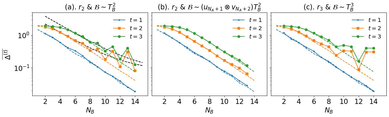
Figure 8: Illustration of $\overline{\Delta^{(t)}}$ versus $N_{B}$ for the first three moments when the measurements are performed in bases largely violating the sufficient condition. In panels (a) and (b), the measurement bases are the eigenbases of $T^{2}_{B}$ and $(u_{N_{A}+1}\otimes v_{N_{A}+1})T^{2}_{B}$, where $T_{B}$ denotes the local translation operator over the subsystem-$B$. We observe that in the former case, the trace distances for higher order moments initially decay and acquire oscillatory behavior around exponential curves decaying to finite non-zero values for larger values of $N_{B}$. Due to the applications of local Haar random unitaries, the behavior in the latter case appears to decay for smaller $N_{B}$ values. However, for larger values of $N_{B}$, we anticipate that the trace distance approaches a finite non-zero value. Panel (c) corresponds to the measurements in the eigenbasis of $T^{3}_{B}.$

Appendix F OBC case

In this appendix, we contrast the initial decay of the trace distances for the PBC case with the OBC case for the same tilted field Ising model. The corresponding results are shown in Fig. 9. In the case where the translational symmetry is absent (OBC), the system has the reflection symmetry only with respect to the central spin. In contrast, for the PBC case, the system has reflection symmetries around every site in addition to the translation symmetry. Due to the periodicity in this case, the entanglement builds up in the time-evolved state at a rate double the case of OBCs. The same is reflected in the phenomenon of emergent state designs.

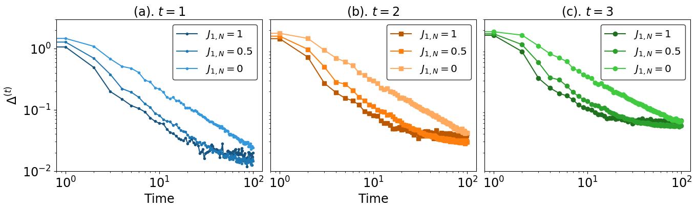
Figure 9: The figure contrasts the decay of $\Delta^{(t)}$ for the state $|0\rangle^{\otimes N}$ evolved under the dynamics of the ising chain with translation symmetry with that of moderately broken translation symmetry and the one with open ends, each characterized by the interaction strength between the first and the $N$-th qubit ($J_{1,N}$). The system size is fixed at $N=18$. The darker colors represent the cases with translation symmetry. The colors blue, orange, and green indicate the first three moments respectively. The size of the projected ensembles $N_{A}$ is fixed at $3$.