Computational Considerations for the Linear Model of Coregionalization

Abstract

In the last two decades, the linear model of coregionalization (LMC) has been widely used to model multivariate spatial processes. From a computational standpoint, the LMC is a substantially easier model to work with than other multidimensional alternatives. Up to now, this fact has been largely overlooked in the literature. Starting from an analogy with matrix normal models, we propose a reformulation of the LMC likelihood that highlights the linear, rather than cubic, computational complexity as a function of the dimension of the response vector. Further, we describe in detail how those simplifications can be included in a Gaussian hierarchical model. In addition, we demonstrate in two examples how the disentangled version of the likelihood we derive can be exploited to improve Markov chain Monte Carlo (MCMC) based computations when conducting Bayesian inference. The first is an interwoven approach that combines samples from centered and whitened parametrizations of the latent LMC distributed random fields. The second is a sparsity-inducing method that introduces structural zeros in the coregionalization matrix in an attempt to reduce the number of parameters in a principled way. It also provides a new way to investigate the strength of the correlation among the components of the outcome vector. Both approaches come at virtually no additional cost and are shown to significantly improve MCMC performance and predictive performance respectively. We apply our methodology to a dataset comprised of air pollutant measurements in the state of California.

Keywords Cross covariance  $\cdot$ Interweaving  $\cdot$ Matrix normal  $\cdot$ Multivariate processes  $\cdot$ Reversible jumps

1 Introduction

The literature concerning computational scalability for spatial Gaussian models has for the most part been concerned with applications where the number of spatial locations $n$ is large. Such situations usually forbid likelihood-based inference because of the ${\mathcal{O}}(n^{3})$ computational cost associated with evaluating the joint normal density. Two of the most prominent approximations used in the applied literature are the stochastic partial differential equation approach pioneered in Lindgren et al. (2011) or the nearest-neighbor methodology (Vecchia, 1988; Datta et al., 2016).

In multivariate spatial models where an output of dimension $p$ is modeled, the cost associated with Gaussian process likelihood evaluations is, in general, ${\mathcal{O}}(p^{3}n^{3})$. While the approximations mentioned above can be extended to multivariate settings in a relatively straightforward manner, they offer no direct computational benefit for cases where the dimensionality $p$ becomes increasingly large. They fall back on the fact that $p\ll n$ in most imaginable scenarios and, legitimately, concentrate on methods that curb the computation as a function of $n$. It is worth mentioning that the concept behind nearest-neighbor processes of pruning the conditional independence graph among locations has also been exploited in Dey et al. (2022) to reduce the computational burden in terms of the dimensionality $p$.

Multivariate spatial models necessitate the specification of a cross-covariance function. Genton and Kleiber (2015) describe the necessary conditions under which such a function will lead to a valid model. They also review some of the most widespread approaches. A lot of those fall under the category of constructive methods in which cross-covariance functions are built from univariate models. Those include the covariance convolution framework (Majumdar and Gelfand, 2007) or the approach based on latent dimensions (Apanasovich and Genton, 2010), among others. Another important example is the class of Matérn cross-covariance functions (Gneiting et al., 2010; Apanasovich et al., 2012) which offers, under some constraints, multivariate spatial models where the marginal distribution of each process has univariate Matérn covariance structure. None of the models mentioned above benefit from the type of computational simplifications we describe in this paper.

Perhaps the simplest (at least conceptually) of multivariate models, the linear model of coregionalization (LMC), is constructed as a linear combination of independent processes. From $r$ orthogonal base processes, we obtain $p$ new components that have cross-dependence. In its inception (Matheron, 1982; Bourgault and Marcotte, 1991; Goulard and Voltz, 1992), the LMC was conceptualized as a mechanism allowing for dimensionality reduction. This is accomplished by specifying a transformation matrix of dimension $p\times r$ with $r<p$. It essentially shrinks an observed $p$-dimensional process to $r$ latent and independent ones. In this work we only discuss the $r=p$ case as most results we describe do not apply otherwise. We exclusively consider the LMC as an approach to construct a $p$-variate process with cross-dependence from $p$ univariate spatial correlation structures as it is described in Schmidt and Gelfand (2003); Gelfand et al. (2004, 2005). The LMC is still used to this day in the applied sciences (see for example Ji et al. (2021); Carter et al. (2022); Heydari et al. (2023)). It is moreover an excellent candidate to incorporate into more involved methodology, such as spatiotemporal models (Mastrantonio et al., 2019; Cappello et al., 2022) or neural network architectures (Liu et al., 2022; Wang et al., 2022).

The LMC implies a likelihood that can be evaluated in a number of operations that is linear in $p$, a fact that has been mostly ignored to this date with few exceptions. This offers immense speed-ups in cases where the number of dimensions is even moderately large. This is not the result of an approximation. Instead, we achieve those computational shortcuts by exploiting the cross-covariance structure implied by the LMC. Hence, there are no drawbacks to utilizing the computational results we present in this paper.

Those computational shortcuts can be viewed as a natural extension of separable models. We review the equivalence between separable models and matrix normal distributions in Section 2. The matrix normal analogy is extended to the general LMC in Section 3. In the context of MCMC-based Bayesian inference, the structure of the LMC can be advantageous beyond the obvious computational speed-ups. In Section 4, we devise an alternate sampler that interweaves (in the sense described in Yu and Meng (2011)) updates to the coregionalization matrix based on two different parametrizations. The goal is to reduce auto-correlation in the posterior samples, specifically for quantities that summarize the cross-correlation structure. Finally, we introduce an alternative prior to the coregionalization matrix in Section 5. This introduces sparsity both in the parameter space and the resulting marginal covariance of the $p$ components, It is shown to significantly improve the accuracy of out-of-sample predictions.

2 The Separable Specification

In this section, we explore the link between multivariate Gaussian processes with a separable cross-covariance function and the matrix normal distribution as defined below. This will serve as an analogy for the computational results we present in Section 3 concerning the general LMC.

Definition 1 (Matrix Normal Distribution (Dawid, 1981)).

A random $p\times n$ matrix $\boldsymbol{\mathrm{X}}$ has the ${\mathcal{M}}{\mathcal{N}}(\boldsymbol{\mathrm{M}},\boldsymbol{\mathrm{\Sigma}},\boldsymbol{\mathrm{R}})$ distribution if its probability density function is given by

$$p(\boldsymbol{\mathrm{X}}|\boldsymbol{\mathrm{M}},\boldsymbol{\mathrm{\Sigma}},\boldsymbol{\mathrm{R}})=\frac{\exp[-\frac{1}{2}\mathrm{tr}\{\boldsymbol{\mathrm{R}}^{-1}(\boldsymbol{\mathrm{X}}-\boldsymbol{\mathrm{M}})^{\top}\boldsymbol{\mathrm{\Sigma}}^{-1}(\boldsymbol{\mathrm{X}}-\boldsymbol{\mathrm{M}})\}]}{(2\pi)^{pn/2}\mathrm{det}(\boldsymbol{\mathrm{R}})^{p/2}\mathrm{det}(\boldsymbol{\mathrm{\Sigma}})^{n/2}},$$ (1)

where $\boldsymbol{\mathrm{M}}$ is a real valued $p\times n$ matrix and $\boldsymbol{\mathrm{\Sigma}},\boldsymbol{\mathrm{R}}$ are respectively $p\times p$ and $n\times n$ positive definite matrices.

Equivalently, $\boldsymbol{\mathrm{X}}\sim{\mathcal{M}}{\mathcal{N}}(\boldsymbol{\mathrm{M}},\boldsymbol{\mathrm{\Sigma}},\boldsymbol{\mathrm{R}})$ if the vector $\mathrm{vec}(\boldsymbol{\mathrm{X}})$ obtained by stacking the columns $\boldsymbol{\mathrm{x}}_{1},\dots,\boldsymbol{\mathrm{x}}_{n}$ of $\boldsymbol{\mathrm{X}}$ has the multivariate normal distribution with mean $\mathrm{vec}(\boldsymbol{\mathrm{M}})$ and covariance $\boldsymbol{\mathrm{R}}\otimes\boldsymbol{\mathrm{\Sigma}}$ where $\otimes$ represents the Kronecker product.

In the previous definition, $\boldsymbol{\mathrm{M}}$ is the location parameter while $\boldsymbol{\mathrm{\Sigma}}$ (resp. $\boldsymbol{\mathrm{R}}$) corresponds to the marginal column (resp. row) covariance. A realization of the ${\mathcal{M}}{\mathcal{N}}(\boldsymbol{\mathrm{M}},\boldsymbol{\mathrm{\Sigma}},\boldsymbol{\mathrm{R}})$ distribution can be obtained from a $p\times n$ matrix $\boldsymbol{\mathrm{Z}}$ of independent standard normal by setting $\boldsymbol{\mathrm{X}}=\boldsymbol{\mathrm{A}}\boldsymbol{\mathrm{Z}}\boldsymbol{\mathrm{B}}^{\top}+\boldsymbol{\mathrm{M}}$ where $\boldsymbol{\mathrm{A}},\boldsymbol{\mathrm{B}}$ are such that $\boldsymbol{\mathrm{\Sigma}}=\boldsymbol{\mathrm{A}}\boldsymbol{\mathrm{A}}^{\top}$ and $\boldsymbol{\mathrm{R}}=\boldsymbol{\mathrm{B}}\boldsymbol{\mathrm{B}}^{\top}$ ($\boldsymbol{\mathrm{A}}$ and $\boldsymbol{\mathrm{B}}$ can be the lower triangular Cholesky factors of $\boldsymbol{\mathrm{\Sigma}}$ and $\boldsymbol{\mathrm{R}}$ for example). Importantly, simulation from such a matrix normal distribution can be accomplished without factorizing the full $np\times np$ matrix $\boldsymbol{\mathrm{R}}\otimes\boldsymbol{\mathrm{\Sigma}}$. The structure of the model allows us to work with individual matrices $\boldsymbol{\mathrm{R}}$ and $\boldsymbol{\mathrm{\Sigma}}$ which will be a common thread in the remainder of this article.

In the spatial modeling context, the equivalent would be to define a multivariate process as $\boldsymbol{\mathrm{v}}(\boldsymbol{\mathrm{s}})=\boldsymbol{\mathrm{A}}\boldsymbol{\mathrm{w}}(\boldsymbol{\mathrm{s}})$ where $\boldsymbol{\mathrm{A}}$ is a $p\times p$ full rank matrix and $\boldsymbol{\mathrm{w}}(\boldsymbol{\mathrm{s}})=(w_{1}(\boldsymbol{\mathrm{s}}),\dots,w_{p}(\boldsymbol{\mathrm{s}}))^{\top}$ consists of $p$ i.i.d. Gaussian random fields. This is known as the LMC with separable covariance structure (Gelfand et al., 2004). We assume that each $w_{j}(\cdot),j=1,\dots,p$ has 0 mean and a marginal variance of 1. Scaling is handled by $\boldsymbol{\mathrm{A}}$ which is referred to as the coregionalization matrix in the following. Let $\boldsymbol{\mathrm{V}}=(\boldsymbol{\mathrm{v}}(\boldsymbol{\mathrm{s}}_{1}),\dots,\boldsymbol{\mathrm{v}}(\boldsymbol{\mathrm{s}}_{n}))$ denote a $p\times n$ matrix organizing in columns some $n$ observations of this multivariate process at distinct locations $s_{1},\dots,s_{n}$ contained in some domain ${\mathcal{S}}$. Commonly, we consider ${\mathcal{S}}\subset\mathds{R}^{2}$ such as in the case of geographically indexed observations. Under the separable specification, the distribution of $\boldsymbol{\mathrm{V}}$ is ${\mathcal{M}}{\mathcal{N}}(\boldsymbol{\mathrm{0}},\boldsymbol{\mathrm{A}}\boldsymbol{\mathrm{A}}^{\top},\boldsymbol{\mathrm{R}})$ where $\boldsymbol{\mathrm{R}}$ is the common correlation matrix associated with the $w_{j}(\cdot)$ processes at locations $\boldsymbol{\mathrm{s}}_{1}.\dots,\boldsymbol{\mathrm{s}}_{n}$. It depends on the coregionalization matrix only through the product $\boldsymbol{\mathrm{A}}\boldsymbol{\mathrm{A}}^{\top}$. Such a process admits a cross-covariance function of the form $C(\boldsymbol{\mathrm{s}},\boldsymbol{\mathrm{t}})=\rho(\boldsymbol{\mathrm{s}},\boldsymbol{\mathrm{t}})\boldsymbol{\mathrm{A}}\boldsymbol{\mathrm{A}}^{T}$, where $\rho(\cdot,\cdot)$ is the common correlation function of processes $w_{j}(\cdot),j=1,\dots,p$. The term separable stems from the fact that the covariance structure factorizes in a spatial component times the marginal (at a single location) covariance among the $p$ dimensions. In this case, inference can be conducted directly on the positive definite matrix $\boldsymbol{\mathrm{\Sigma}}=\boldsymbol{\mathrm{A}}\boldsymbol{\mathrm{A}}^{\top}$ rather than the non-identifiable $\boldsymbol{\mathrm{A}}$. The remaining parameters are those contained in the common spatial correlation function defining the processes $w_{j}(\cdot),j=1,\dots,p$. We assume the correlation between two locations $\boldsymbol{\mathrm{s}},\boldsymbol{\mathrm{t}}$ to be of the form $\rho(\varphi|\boldsymbol{\mathrm{s}}-\boldsymbol{\mathrm{t}}|)$ where $\rho(\cdot)$ is some positive definite function. For ease of exposition, the spatial dependence is encapsulated by a single range parameter $\varphi>0$. More elaborate families could also be envisioned.

We focus on a Bayesian formulation of inference and consider an MCMC approach that updates parameters $\boldsymbol{\mathrm{\Sigma}}$ and $\varphi$ in turn at each iteration. This usually entails evaluating the likelihood at each step of the Markov chain which is known to be costly for multivariate Gaussian densities even with a moderate sample size. If we were to naively consider the multivariate normal distribution of $\mathrm{vec}(\boldsymbol{\mathrm{V}})$, evaluating the likelihood would require computing the inverse and determinant of the covariance matrix $\boldsymbol{\mathrm{R}}\otimes\boldsymbol{\mathrm{\Sigma}}$. This computation has overall ${\mathcal{O}}(p^{3}n^{3})$ asymptotic complexity. However, basic algebra results tell us that $(\boldsymbol{\mathrm{R}}\otimes\boldsymbol{\mathrm{\Sigma}})^{-1}=\boldsymbol{\mathrm{R}}^{-1}\otimes\boldsymbol{\mathrm{\Sigma}}^{-1}$ and $\mathrm{det}(\boldsymbol{\mathrm{R}}\otimes\boldsymbol{\mathrm{\Sigma}})=\mathrm{det}(\boldsymbol{\mathrm{R}})^{p}\mathrm{det}(\boldsymbol{\mathrm{\Sigma}})^{n}$. Exploiting the structure of this model allows us to conduct our calculation directly on the individual matrices $\boldsymbol{\mathrm{R}}$ and, $\boldsymbol{\mathrm{\Sigma}}$ which is a great advantage over a general multivariate model for a sample size of $np$. An update to the single spatial range parameter $\varphi$ requires us to compute the inverse and determinant of the $n\times n$ matrix $\boldsymbol{\mathrm{R}}$ which is the crux of the computation since we consider the number $n$ of samples to greatly exceed the dimension $p$ of each observation, i.e. $p\ll n$.

Moreover, we can rewrite the quadratic product $\mathrm{vec}(\boldsymbol{\mathrm{V}})^{\top}(\boldsymbol{\mathrm{R}}^{-1}\otimes\boldsymbol{\mathrm{\Sigma}}^{-1})\mathrm{vec}(\boldsymbol{\mathrm{V}})$ as a trace to obtain an expression similar to equation (1), thus avoiding the need to ever construct or store any $np\times np$ matrix. What is also worth mentioning is that we obtain full-conditional conjugacy by assigning an inverse-Wishart prior to $\boldsymbol{\mathrm{\Sigma}}$. Those computational considerations about the separable model are exposed in Banerjee and Gelfand (2002) among others. We solely review them here to provide some context for the more general results we present in Section 3.

However, from a modeling perspective, the separable specification is too restrictive for most applications as the components of $\boldsymbol{\mathrm{v}}(\cdot)$ have the same marginal distribution. In particular, it would imply that all the variables in the model have the same practical range. This assumption is pretty strong and rather unreasonable when modeling the spatial covariation of different environmental variables, for example. In spatiotemporal settings, separability is often assumed among spatial and time dependence. In other words, it makes sense to consider the marginal spatial dependence to be the same at any fixed time. Multivariate dynamical models in the context of the LMC are discussed in Gelfand et al. (2005).

3 The General LMC

Allowing the independent base processes $w_{j}(\cdot),j=1,\dots,p$ to have distinct covariance functions solves the issue of having identically distributed components $v_{j}(\cdot)$. In light of Section 2, a natural question that arises is how much, if any, of the computational advantages can be retained from the separable case. The essence of the computational result we propose was briefly discussed in the Ph.D. thesis of Kyzyurova (2017). To summarize, the covariance structure of the LMC implies Gaussian likelihood evaluations that scale linearly in $p$ rather than the ${\mathcal{O}}(p^{3}n^{3})$ associated with general multivariate models. It positions the LMC as a computationally advantageous alternative to other multivariate processes. In our opinion, this fact has failed to gain the traction it deserves.

The setup is as before, with a multivariate process $\boldsymbol{\mathrm{v}}(\boldsymbol{\mathrm{s}})$ defined from $p$ independent processes $w_{j}(\boldsymbol{\mathrm{s}}),j=1,\dots,p$ through the linear transformation $\boldsymbol{\mathrm{v}}(\boldsymbol{\mathrm{s}})=\boldsymbol{\mathrm{A}}\boldsymbol{\mathrm{w}}(\boldsymbol{\mathrm{s}})$. This time, however, the base processes $w_{j}(\cdot)$ do not have the same distribution. As before, we consider the processes to have a mean of 0 and a variance of 1, but we make them distinct by assigning each $w_{j}(\cdot)$ a different correlation function $\rho_{j}(\cdot)$ (Schmidt and Gelfand, 2003). We will restrict ourselves to one family of isotropic and stationary correlation functions indexed by distinct range parameters so that $\mathrm{Cov}(w_{j}(\boldsymbol{\mathrm{s}}),w_{j}(\boldsymbol{\mathrm{t}}))=\rho_{j}(\boldsymbol{\mathrm{s}},\boldsymbol{\mathrm{t}})=\rho(\varphi_{j}|\boldsymbol{\mathrm{s}}-\boldsymbol{\mathrm{t}}|)$.

Gaussian distribution properties under linear transformations tell us that the cross-covariance function of the multivariate process $\boldsymbol{\mathrm{v}}(\cdot)$ is given by, $C(\boldsymbol{\mathrm{s}},\boldsymbol{\mathrm{t}})=\sum_{j=1}^{p}\rho_{j}(\boldsymbol{\mathrm{s}},\boldsymbol{\mathrm{t}})\boldsymbol{\mathrm{a}}_{j}\boldsymbol{\mathrm{a}}_{j}^{\top}$ where $\boldsymbol{\mathrm{a}}_{j}$ is the $j^{\mathrm{th}}$ column of $\boldsymbol{\mathrm{A}}$. For a finite sample of size $n$ organized in a column vector $(\boldsymbol{\mathrm{v}}(\boldsymbol{\mathrm{s}}_{1})^{\top},\dots,\boldsymbol{\mathrm{v}}(\boldsymbol{\mathrm{s}}_{n})^{\top})^{\top}$ of length $np$, this equates to a multivariate normal distribution of mean 0 and covariance matrix $\sum_{j=1}^{p}\boldsymbol{\mathrm{R}}_{j}\otimes\boldsymbol{\mathrm{a}}_{j}\boldsymbol{\mathrm{a}}_{j}^{\top}$ (Gelfand et al., 2004) with $\boldsymbol{\mathrm{R}}_{j}$ being the spatial correlation matrix associated with $(w_{j}(\boldsymbol{\mathrm{s}}_{1}),\dots,w_{j}(\boldsymbol{\mathrm{s}}_{n}))^{\top}$.

Neither the covariance function nor matrix can be factorized under the general LMC so it is unclear how the structure of the model could be exploited. On the other hand, we know intuitively that generating LMC-distributed random variables does not require the Cholesky factor of the $np\times np$ covariance matrix. We can simulate the base point processes $w_{j}(\cdot)$ at locations $\boldsymbol{\mathrm{s}}_{1},\dots,\boldsymbol{\mathrm{s}}_{n}$ from the individual Cholesky factors ($\boldsymbol{\mathrm{B}}_{j}$, say) of the spatial correlation matrices $\boldsymbol{\mathrm{R}}_{j},j=1\dots,p$ and then apply the linear transformation $\boldsymbol{\mathrm{A}}$ at every location. In algebraic terms, we can generate an $p\times n$ LMC distributed matrix $\boldsymbol{\mathrm{V}}$ with rows (resp. columns) corresponding to processes (resp. locations) by setting

$$\boldsymbol{\mathrm{V}}=\sum_{j=1}^{p}\boldsymbol{\mathrm{a}}_{j}\boldsymbol{\mathrm{z}}_{j}\boldsymbol{\mathrm{B}}_{j}^{\top},$$

where $\boldsymbol{\mathrm{z}}_{j}$ are row vectors of independent and standard normal random variables. Just as we can circumvent the factorization of the $np\times np$ covariance matrix when simulating the LMC, we can also avoid computing the inverse and determinant directly when evaluating the likelihood.

In appendix A, we detail the following two results which have appeared in Kyzyurova (2017) under some slightly different notation. The first one tells us how to compute the precision matrix: $(\sum_{j=1}^{p}\boldsymbol{\mathrm{R}}_{j}\otimes\boldsymbol{\mathrm{a}}_{j}\boldsymbol{\mathrm{a}}_{j}^{\top})^{-1}=\sum_{j=1}^{p}\boldsymbol{\mathrm{R}}_{j}^{-1}\otimes\boldsymbol{\mathrm{a}}_{j}^{-\top}\boldsymbol{\mathrm{a}}_{j}^{-1}$, where $\boldsymbol{\mathrm{a}}_{j}^{-1}$ is the $j^{\mathrm{th}}$ line of the inverse matrix $\boldsymbol{\mathrm{A}}^{-1}$. The second one concerns the determinant and says that $\mathrm{det}(\sum_{j=1}^{p}\boldsymbol{\mathrm{R}}_{j}\otimes\boldsymbol{\mathrm{a}}_{j}\boldsymbol{\mathrm{a}}_{j}^{\top})=\mathrm{det}(\boldsymbol{\mathrm{A}})^{2n}\prod_{j=1}^{p}\mathrm{det}(\boldsymbol{\mathrm{R}}_{j})$. We go a little bit further and express the LMC likelihood in terms of the $p\times n$ matrix $\boldsymbol{\mathrm{V}}$. This facilitates the calculation a little beyond what is shown in Kyzyurova (2017) by simplifying what would be a $np\times np$ quadratic product under the vectorized form.

Proposition 1 (The LMC Density).

Let $\boldsymbol{\mathrm{w}}_{j}\stackrel{{\scriptstyle\text{ind.}}}{{\sim}}{\mathcal{N}}(\boldsymbol{\mathrm{0}},\boldsymbol{\mathrm{R}}_{j}),j=1,\dots,p$ be independent $n$-vectors forming the lines of the $p\times n$ matrix $\boldsymbol{\mathrm{W}}=(\boldsymbol{\mathrm{w}}_{1},\dots,\boldsymbol{\mathrm{w}}_{p})^{\top}$. The random matrix $\boldsymbol{\mathrm{V}}=\boldsymbol{\mathrm{A}}\boldsymbol{\mathrm{W}}$ (for some $p\times p$ full-rank matrix $\boldsymbol{\mathrm{A}}$) has a probability density function

$$p(\boldsymbol{\mathrm{V}}|\boldsymbol{\mathrm{A}},\boldsymbol{\mathrm{R}}_{j=1}^{p})=\frac{\exp[-\frac{1}{2}\sum_{j=1}^{p}\boldsymbol{\mathrm{a}}_{j}^{-1}\boldsymbol{\mathrm{V}}\boldsymbol{\mathrm{R}}_{j}^{-1}\boldsymbol{\mathrm{V}}^{\top}\boldsymbol{\mathrm{a}}_{j}^{-\top}]}{(2\pi)^{np/2}|\mathrm{det}(\boldsymbol{\mathrm{A}})|^{n}\prod_{j=1}^{p}\mathrm{det}(\boldsymbol{\mathrm{R}}_{j})^{1/2}}.$$ (2)

Equivalently, we write $\boldsymbol{\mathrm{V}}\sim{\text{LMC}}(\boldsymbol{\mathrm{A}},\boldsymbol{\mathrm{R}}_{j=1}^{p})$ if $\mathrm{vec}(\boldsymbol{\mathrm{V}})$ has the multivariate normal distribution with mean $\boldsymbol{\mathrm{0}}$ and covariance $\sum_{j=1}^{p}\boldsymbol{\mathrm{R}}_{j}\otimes\boldsymbol{\mathrm{a}}_{j}\boldsymbol{\mathrm{a}}_{j}^{\top}$ with $\boldsymbol{\mathrm{A}}=(\boldsymbol{\mathrm{a}}_{1},\dots,\boldsymbol{\mathrm{a}}_{p})$.

Expression (2) is analogous (in the case of the general LMC) to the matrix normal density in equation (1). We can see that it is again possible to evaluate the likelihood of $\boldsymbol{\mathrm{V}}$ without computing the determinant or inverse of any $np\times np$ matrix neither is it necessary to store any such matrix. Computation can be carried out directly on the coregionalization matrix $\boldsymbol{\mathrm{A}}$ and the $p$ spatial correlation matrices $\boldsymbol{\mathrm{R}}_{j}$ obtained by applying the functions $\rho(\varphi_{j}|\cdot|)$ to all pairs of locations in $\boldsymbol{\mathrm{s}}_{1},\dots,\boldsymbol{\mathrm{s}}_{n}$. In Figure 1, we empirically compare how likelihood computations scale: we can see the polynomial trend (as a function of $p$) of the naive vectorized form compared to the likelihood formulation in (2) which is linear in $p$ as expected.

Figure 1: Time elapsed after 500 likelihood evaluations for corresponding $n$ and $p$. The matrix form of the likelihood is the one described in Proposition 1 while the vector form is the naive implementation that computes both the determinant and inverse of $\sum_{j=1}^{p}\boldsymbol{\mathrm{R}}_{j}\otimes\boldsymbol{\mathrm{a}}_{j}\boldsymbol{\mathrm{a}}_{j}^{\top}$.

Marginally, the covariance matrix of the process $\boldsymbol{\mathrm{v}}(\boldsymbol{\mathrm{s}})$ at a single location $\boldsymbol{\mathrm{s}}$ is $\boldsymbol{\mathrm{A}}\boldsymbol{\mathrm{A}}^{\top}$ since the $\boldsymbol{\mathrm{w}}_{j}(\cdot)$ processes have a variance of 1. However, unlike in the separable case, the finite sample distribution is not the same in general for two different coregionalization matrices $\boldsymbol{\mathrm{A}}_{1},\boldsymbol{\mathrm{A}}_{2}$ even if $\boldsymbol{\mathrm{A}}_{1}\boldsymbol{\mathrm{A}}_{1}^{\top}=\boldsymbol{\mathrm{A}}_{2}\boldsymbol{\mathrm{A}}_{2}^{\top}$ (see Appendix B). There are still however identifiability issues with the matrix $\boldsymbol{\mathrm{A}}$ in the covariance matrix $\sum_{j=1}^{p}\boldsymbol{\mathrm{R}}_{j}\otimes\boldsymbol{\mathrm{a}}_{j}\boldsymbol{\mathrm{a}}_{j}^{\top}$. The model is equivalent even if we apply a change of sign to any column $\boldsymbol{\mathrm{a}}_{j}$. It is also invariant under any reordering/relabelling of indices $\{1,\dots,p\}$. The general LMC implies a covariance among pairs of scalar observations that is of the form

$$\mathrm{Cov}(v_{i}(\boldsymbol{\mathrm{s}}_{1}),v_{j}(\boldsymbol{\mathrm{s}}_{2}))=C_{ij}(\boldsymbol{\mathrm{s}}_{1},\boldsymbol{\mathrm{s}}_{2})=\sum_{k=1}^{p}a_{ik}a_{jk}\rho(\varphi_{k}|\boldsymbol{\mathrm{s}}_{1}-\boldsymbol{\mathrm{s}}_{2}|),$$ (3)

where the quantities $a_{ij}$ are the individual entries in the coregionalization matrix $\boldsymbol{\mathrm{A}}$. An example of a bivariate realization along with the corresponding cross-covariance function is illustrated in Figure 2. In Appendix C, we describe in more detail how the cross-covariance function described by 3 compares with other well-known alternatives (computational considerations aside).

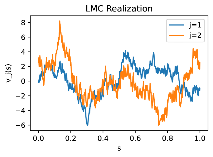
(a)

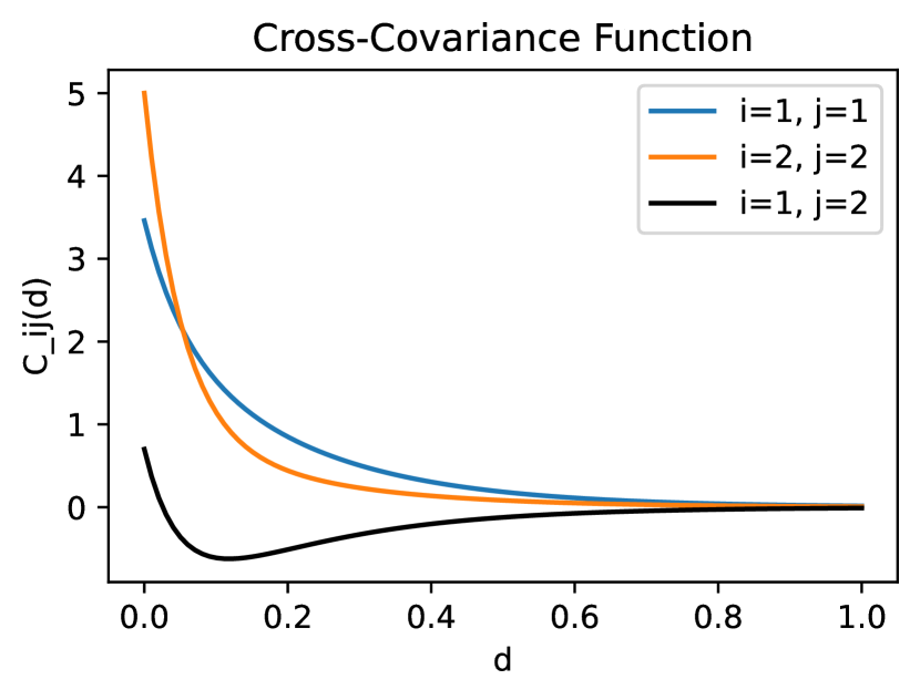
(b)

Figure 2: (a) Trajectories of a bivariate Gaussian process over $[0,1]$ with covariance structure illustrated in (b). The two processes are positively correlated at very short distances but otherwise negatively correlated with the lowest point being around $s=0.1$.

Next, we discuss predicting the multivariate process implied by the LMC at a set $\boldsymbol{\mathrm{s}}_{\mathrm{PRED}}$ of locations conditional on its values observed at locations $\boldsymbol{\mathrm{s}}_{\mathrm{OBS}}$. We start by describing the conditional distributions of the LMC. Same as before, we assume $\boldsymbol{\mathrm{V}}$ is a $p\times n$ matrix, only this time the matrix is split along the horizontal into 2 sub-matrices $\boldsymbol{\mathrm{V}}_{\mathrm{OBS}}$ and $\boldsymbol{\mathrm{V}}_{\mathrm{PRED}}$ such that $\boldsymbol{\mathrm{V}}=(\boldsymbol{\mathrm{V}}_{\mathrm{OBS}},\boldsymbol{\mathrm{V}}_{\mathrm{PRED}})$. In that case, the spatial correlation matrices $\boldsymbol{\mathrm{R}}_{j}$ are each partitioned between old and new locations, as

$$\boldsymbol{\mathrm{R}}_{j}=\left(\begin{matrix}[l]\boldsymbol{\mathrm{R}}^{(j)}_{\mathrm{OBS}}&\boldsymbol{\mathrm{R}}^{(j)}_{\mathrm{OBS},\mathrm{PRED}}\\ \boldsymbol{\mathrm{R}}^{(j)}_{\mathrm{PRED},\mathrm{OBS}}&\boldsymbol{\mathrm{R}}^{(j)}_{\mathrm{PRED}}\end{matrix}\right).$$ (4)

We are interested in the conditional distribution of $\boldsymbol{\mathrm{V}}_{\mathrm{PRED}}$ given $\boldsymbol{\mathrm{V}}_{\mathrm{OBS}}$. Importantly, the distribution of $\boldsymbol{\mathrm{V}}_{\mathrm{PRED}}$ conditional on $\boldsymbol{\mathrm{V}}_{\mathrm{OBS}}$ is Gaussian, as expected, but also preserves the LMC covariance structure. This is detailed in the following result.

Proposition 2 (Conditional Distributions of the LMC).

The distribution implied by the LMC at locations $\boldsymbol{\mathrm{s}}_{\mathrm{PRED}}$ conditional on its values $\boldsymbol{\mathrm{V}}_{\mathrm{OBS}}$ at locations $\boldsymbol{\mathrm{s}}_{\mathrm{OBS}}$ is also an LMC with coregionalization matrix $\boldsymbol{\mathrm{A}}$ and spatial correlation matrices given by $\boldsymbol{\mathrm{R}}^{(j)}_{\mathrm{PRED}}-\boldsymbol{\mathrm{R}}^{(j)}_{\mathrm{PRED},\mathrm{OBS}}{\boldsymbol{\mathrm{R}}^{(j)^{-1}}_{\mathrm{OBS}}}\boldsymbol{\mathrm{R}}^{(j)}_{\mathrm{OBS},\mathrm{PRED}}$. It is centered around the matrix

$$\sum_{j=1}^{p}\boldsymbol{\mathrm{a}}_{j}\boldsymbol{\mathrm{a}}_{j}^{-1}\boldsymbol{\mathrm{V}}_{\mathrm{OBS}}{\boldsymbol{\mathrm{R}}^{(j)^{-1}}_{\mathrm{OBS}}}\boldsymbol{\mathrm{R}}^{(j)}_{\mathrm{OBS},\mathrm{PRED}}.$$ (5)

This is equivalent to applying the inverse transformation $\boldsymbol{\mathrm{A}}^{-1}\boldsymbol{\mathrm{V}}_{\mathrm{OBS}}=\boldsymbol{\mathrm{W}}_{\mathrm{OBS}}$, computing the conditional $\boldsymbol{\mathrm{W}}_{\mathrm{PRED}}$ across the $p$ independent rows and transforming back as $\boldsymbol{\mathrm{V}}_{\mathrm{PRED}}=\boldsymbol{\mathrm{A}}\boldsymbol{\mathrm{W}}_{\mathrm{PRED}}$.

The proof can be found in Appendix D. Proposition 2 has implications for Vecchia type of approximations (Vecchia, 1988; Datta et al., 2016; Katzfuss and Guinness, 2021) which are described by conditional independence assumptions. This computational approximation offers likelihood evaluations that are linear in the number $n$ of locations. It also has been shown empirically to be accurate when compared with alternative methods (Heaton et al., 2019). That the LMC covariance structure is preserved under conditioning signifies that the computational benefits we describe here can in principle be used in conjunction with such approximations when both $n$ and $p$ are fairly large.

3.1 The triangular specification

A common thread among the statistical literature concerning the LMC (see Schmidt and Gelfand (2003); Foley and Fuentes (2008) for example) is to use a lower triangular parametrization for the coregionalization matrix $\boldsymbol{\mathrm{A}}$ where diagonal elements are restricted to positive values. It does solve the identifiability issue described in the previous section. Columns cannot change signs anymore because of the positivity of the diagonal. They cannot be reordered, either, since that would break the triangular structure.

Doing so, however, imposes an asymmetry on the components of the model. The modeling assumptions are different under a reordering of dimension indices, $\{1,\dots,p\}$ even though we usually think of such labels as superfluous. It is perhaps better appreciated by looking at the marginal covariance function implied by the lower triangular structure. For each process $v_{j}(\cdot),j=1,\dots,p$, we have from (3) that

$$C_{1}(\boldsymbol{\mathrm{s}},\boldsymbol{\mathrm{t}}) =a_{11}^{2}\rho(\varphi_{1}|\boldsymbol{\mathrm{s}}-\boldsymbol{\mathrm{t}}|),$$

$$C_{2}(\boldsymbol{\mathrm{s}},\boldsymbol{\mathrm{t}}) =a_{21}^{2}\rho(\varphi_{1}|\boldsymbol{\mathrm{s}}-\boldsymbol{\mathrm{t}}|)+a_{22}^{2}\rho(\varphi_{2}|\boldsymbol{\mathrm{s}}-\boldsymbol{\mathrm{t}}|),$$

$$\vdots$$

$$C_{p}(\boldsymbol{\mathrm{s}},\boldsymbol{\mathrm{t}}) =\sum_{k=1}^{p}a_{pk}^{2}\rho(\varphi_{k}|\boldsymbol{\mathrm{s}}-\boldsymbol{\mathrm{t}}|).$$

We can see the marginal models go up in complexity as indices increase. This limitation is also outlined in Carter et al. (2022).

As discussed in Schmidt and Gelfand (2003) and Gelfand et al. (2004), the lower triangular specification for $\boldsymbol{\mathrm{A}}$ admits a computational simplification when describing the processes conditionally as $v_{j}(\boldsymbol{\mathrm{s}})|v_{1}(\boldsymbol{\mathrm{s}}),\dots,v_{j-1}(\boldsymbol{\mathrm{s}})$. This arises because we can write $\boldsymbol{\mathrm{A}}^{-1}\boldsymbol{\mathrm{v}}(\boldsymbol{\mathrm{s}})=\boldsymbol{\mathrm{w}}(\boldsymbol{\mathrm{s}})$ and $\boldsymbol{\mathrm{A}}^{-1}$ is also lower triangular. Hence, for any $j=1,\dots,p$ we can write $v_{j}(\boldsymbol{\mathrm{s}})=\sum_{\ell=1}^{j-1}\alpha_{j\ell}v_{\ell}(\boldsymbol{\mathrm{s}})+\sigma_{j}w(\boldsymbol{\mathrm{s}})$ with $\alpha_{j\ell}=-a^{-1}_{j\ell}/a^{-1}_{jj}$ and $\sigma_{j}=1/a^{-1}_{jj}$ ($a^{-1}_{j\ell}$ are elements of the inverse matrix $\boldsymbol{\mathrm{A}}^{-1}$). Each process $v_{j}(\boldsymbol{\mathrm{s}})$ is a linear combination of the previous $v_{1}(\boldsymbol{\mathrm{s}}),\dots,v_{j-1}(\boldsymbol{\mathrm{s}})$ and the $j^{\text{th}}$ underlying process $w_{j}(\boldsymbol{\mathrm{s}})$. The covariance matrix of process $v_{j}(\cdot)$ at locations $\boldsymbol{\mathrm{s}}_{1},\dots,\boldsymbol{\mathrm{s}}_{n}$ conditional on previous $v_{\ell}(\cdot),\ell=1,\dots,j-1$ simplifies to that of $w_{j}(\cdot)$ at said locations.

To summarize, the likelihood can be computed in conditional factorization from the inverses and determinants of individual matrices $\boldsymbol{\mathrm{A}},\boldsymbol{\mathrm{R}}_{1},\dots,\boldsymbol{\mathrm{R}}_{p}$. This is an attractive formulation from a computational standpoint. Generalizing this, we demonstrated in Section 3 that any LMC parametrization benefits from a similar computational simplification. This is fortunate as the triangular approach is limiting and hard to justify. It is a fundamental (rather than circumstantial) property of the LMC to have likelihood evaluations that require a number of operations that is linear in $p$. Computational simplicity is perhaps its most attractive feature.

4 Hierarchical Models

In this section, we stir away from the approach of Kyzyurova (2017) and consider the LMC as part of a proper statistical setup rather than in the realm of computer models. We first describe what is a standard problem when discussing computational scalability in any Gaussian process model. Suppose you observe a process $\boldsymbol{\mathrm{Y}}(\boldsymbol{\mathrm{s}})=\boldsymbol{\mathrm{v}}(\boldsymbol{\mathrm{s}})+\boldsymbol{\mathrm{\epsilon}}(\boldsymbol{\mathrm{s}})$ where $\boldsymbol{\mathrm{v}}(\cdot)$ is some zero mean process accounting for spatial dependence in ${\mathcal{S}}\subset\mathds{R}^{d}$ space while $\epsilon(\cdot)$ is some form of white noise. The multivariate ${\mathcal{N}}(0,\boldsymbol{\mathrm{\Sigma}})$ distribution implied by process $\boldsymbol{\mathrm{v}}(\cdot)$ observed at locations $\boldsymbol{\mathrm{s}}_{1},\dots,\boldsymbol{\mathrm{s}}_{n}$ might benefit from some useful computational tricks when computing the likelihood. This could be the result of employing an approximation such as the nearest neighbor approach ofDatta et al. (2016) that provides a factorization (detailed in Finley et al. (2019)) of the precision matrix $\boldsymbol{\mathrm{\Sigma}}^{-1}$. It could also be because the covariance structure of $\boldsymbol{\mathrm{\Sigma}}$ can be exploited, as is the case for the LMC.

In either case, we face the same problem: the finite-dimensional distribution of $\boldsymbol{\mathrm{Y}}(\cdot)$ observed at $n$ locations will be of the form ${\mathcal{N}}(0,\boldsymbol{\mathrm{\Sigma}}+\boldsymbol{\mathrm{D}})$ for some diagonal matrix $\boldsymbol{\mathrm{D}}$. Since $\boldsymbol{\mathrm{D}}$ is of full rank, there is no simple way to evaluate the Gaussian likelihood without inverting or computing the determinant of any $np\times np$ matrix (in the multivariate setting). In other words, working with the distribution of the collapsed Gaussian process $\boldsymbol{\mathrm{Y}}(\boldsymbol{\mathrm{s}})$ forces you to relinquish any computational schemes that applied to $\boldsymbol{\mathrm{v}}(\boldsymbol{\mathrm{s}})$.

In a Bayesian context, there is always the option of sampling the latent random field $\boldsymbol{\mathrm{v}}(\cdot)$ and model parameters in turn in a Gibbs sampling approach. However, this often leads to Markov chains that exhibit high autocorrelation Papaspiliopoulos et al. (2007); Murray and Adams (2010); Yu and Meng (2011). We explore strategies to alleviate this problem for the specific case of the LMC in the following section. The distribution of $\boldsymbol{\mathrm{v}}$ conditional on $\boldsymbol{\mathrm{y}}$ is multivariate normal with covariance matrix, $(\boldsymbol{\mathrm{\Sigma}}^{-1}+\boldsymbol{\mathrm{D}}^{-1})^{-1}$ which is also cumbersome to work with. Nevertheless, sampling from the full conditionals of the $np$-dimensional distribution of $\boldsymbol{\mathrm{v}}|\boldsymbol{\mathrm{y}}$ can be accomplished without the need to invert or factorize any $np\times np$ matrix. Details are given in Appendix E.

In the context of the LMC, the finite sample equation has the form $\boldsymbol{\mathrm{Y}}=\boldsymbol{\mathrm{V}}+\boldsymbol{\mathrm{\epsilon}}$ where $\boldsymbol{\mathrm{V}}\sim{\text{LMC}}(\boldsymbol{\mathrm{A}},\boldsymbol{\mathrm{R}}_{j=1}^{p})$ and $\epsilon\sim{\mathcal{M}}{\mathcal{N}}(\boldsymbol{\mathrm{0}},\boldsymbol{\mathrm{D}},\boldsymbol{\mathrm{I}})$. The $p\times p$ matrix $\boldsymbol{\mathrm{D}}=\text{diag}\{\tau_{j},j=1,\dots,p\}$ contains the distinct observational variances associated with each of the $p$ processes. We omit the usual mean structure to focus our discussion on the sampling of covariance parameters. The LMC structure of $\boldsymbol{\mathrm{V}}$ cannot be exploited for deriving the covariance of, $\boldsymbol{\mathrm{Y}}$ even though $\boldsymbol{\mathrm{\epsilon}}$ is itself an LMC distributed matrix normal. In general, the sum of LMC-distributed matrices is not itself distributed according to the LMC. The same is true for the standard matrix normal distribution described by Definition 1.

The $2np$-dimensional normal density of the complete data $\boldsymbol{\mathrm{Y}},\boldsymbol{\mathrm{V}}$ is of the form:

$$p(\boldsymbol{\mathrm{Y}},\boldsymbol{\mathrm{V}}|\boldsymbol{\mathrm{A}},\boldsymbol{\mathrm{R}}_{j=1}^{p},\boldsymbol{\mathrm{D}})=\frac{\exp[-\frac{1}{2}\sum_{j=1}^{p}\boldsymbol{\mathrm{a}}_{j}^{-1}\boldsymbol{\mathrm{V}}\boldsymbol{\mathrm{R}}_{j}^{-1}\boldsymbol{\mathrm{V}}^{\top}\boldsymbol{\mathrm{a}}_{j}^{-\top}-\frac{1}{2}\mathrm{tr}\{(\boldsymbol{\mathrm{V}}-\boldsymbol{\mathrm{Y}})^{\top}\boldsymbol{\mathrm{D}}^{-1}(\boldsymbol{\mathrm{V}}-\boldsymbol{\mathrm{Y}})\}]}{(2\pi)^{np}|\mathrm{det}(\boldsymbol{\mathrm{A}})|^{n}\prod_{j=1}^{p}\mathrm{det}(\boldsymbol{\mathrm{R}}_{j})^{1/2}\prod_{j=1}^{p}\tau_{j}^{n/2}}.$$ (6)

Because we used the alternative formulation described in Section 3 for the latent LMC $\boldsymbol{\mathrm{V}}$, expression (6) above can be evaluated without the need to carry out computations on any $np\times np$ matrices.

The complete data likelihood in (6) describes a hierarchical model for $\boldsymbol{\mathrm{Y}}$ that is centered at $\boldsymbol{\mathrm{V}}$ with independent error terms $\boldsymbol{\mathrm{\epsilon}}$. Fittingly, we will refer to this context as the centered parameterization (Papaspiliopoulos et al., 2007). Alternatively, we could also write $\boldsymbol{\mathrm{Y}}=\boldsymbol{\mathrm{A}}\boldsymbol{\mathrm{W}}+\boldsymbol{\mathrm{\epsilon}}$ where $\boldsymbol{\mathrm{W}}\sim{\text{LMC}}(\boldsymbol{\mathrm{I}},\boldsymbol{\mathrm{R}}_{j=1}^{p})$. The rows $\boldsymbol{\mathrm{w}}_{1},\boldsymbol{\mathrm{w}}_{2},\dots,\boldsymbol{\mathrm{w}}_{p}$ of $\boldsymbol{\mathrm{W}}$ are the $p$ independent spatial processes underlying the LMC. In this context, the latent process $\boldsymbol{\mathrm{W}}$ is a priori independent of the coregionalization matrix $\boldsymbol{\mathrm{A}}$. We refer to this setup as the whitened parametrization (Murray and Adams, 2010). In essence, since the latent process $\boldsymbol{\mathrm{V}}$ is not observed, we can equivalently think of the complete data as $(\boldsymbol{\mathrm{Y}},\boldsymbol{\mathrm{W}})$. This leads to a joint likelihood of the form

$$p(\boldsymbol{\mathrm{Y}},\boldsymbol{\mathrm{W}}|\boldsymbol{\mathrm{A}},\boldsymbol{\mathrm{R}}_{j=1}^{p},\boldsymbol{\mathrm{D}})=\frac{\exp[-\frac{1}{2}\sum_{j=1}^{p}\boldsymbol{\mathrm{w}}_{j}^{\top}\boldsymbol{\mathrm{R}}_{j}^{-1}\boldsymbol{\mathrm{w}}_{j}-\frac{1}{2}\mathrm{tr}\{(\boldsymbol{\mathrm{A}}\boldsymbol{\mathrm{W}}-\boldsymbol{\mathrm{Y}})^{\top}\boldsymbol{\mathrm{D}}^{-1}(\boldsymbol{\mathrm{A}}\boldsymbol{\mathrm{W}}-\boldsymbol{\mathrm{Y}})\}]}{(2\pi)^{np}\prod_{j=1}^{p}\mathrm{det}(\boldsymbol{\mathrm{R}}_{j})^{1/2}\prod_{j=1}^{p}\tau_{j}^{n/2}}.$$ (7)

Expression (7), same as (6), factorizes in individual terms containing inverses or determinants of potentially large correlation matrices $\boldsymbol{\mathrm{R}}_{j}$. Those represent the crux of the computation when evaluating the likelihood. It seems we can benefit from similar computational advantages to those described in Section 3 by simply changing the parametrization.

However, in the context where the independent variance terms $\tau_{j}$ along the diagonal of $\boldsymbol{\mathrm{D}}$ are small, updates to $\boldsymbol{\mathrm{A}}$ conditional on fixed $\boldsymbol{\mathrm{W}}$ will tend to be very concentrated around the current value. Gibbs samplers that alternate updates to the latent variables $\boldsymbol{\mathrm{W}}$ and model parameters $\boldsymbol{\mathrm{A}},\varphi_{j=1}^{p},\tau_{j=1}^{p}$ are likely to exhibit high autocorrelation in the components of $\boldsymbol{\mathrm{A}}$ for reasons that are well outlined in Murray and Adams (2010). In other words, such a formulation of the problem is unlikely to perform very well when the signal-to-noise (StN) ratio is relatively high. In return, it is likely to perform better than the centered parametrization in the context where the StN ratio is low. However, such a scenario is not auspicious for statistical analysis in general. In the next section, we explore interweaving strategies that can, in principle, benefit from the advantages of both parametrizations.

4.1 Interweaving

Components of the model are $\boldsymbol{\mathrm{V}},\boldsymbol{\mathrm{W}},\boldsymbol{\mathrm{A}},\varphi_{j=1}^{p},\tau_{j=1}^{p}$. Model parameters are $\boldsymbol{\mathrm{A}},\varphi_{j=1}^{p},\tau_{j=1}^{p}$ while $\boldsymbol{\mathrm{V}},\boldsymbol{\mathrm{W}}$ are equivalent representations of the latent LMC linked by the 1 to 1 transformation $\boldsymbol{\mathrm{V}}=\boldsymbol{\mathrm{A}}\boldsymbol{\mathrm{W}}$. In the example we present below, we put independent Gaussian priors on the elements of the coregionalization matrix $\boldsymbol{\mathrm{A}}$. We use the exponential correlation function $\rho(\varphi_{j}|\boldsymbol{\mathrm{s}}-\boldsymbol{\mathrm{t}}|)=\exp(-\varphi_{j}|\boldsymbol{\mathrm{s}}-\boldsymbol{\mathrm{t}}|)$ for the underlying process $w_{j}(\cdot)$ and the range parameters $\varphi_{1},\dots,\varphi_{p}$ are assigned uniform priors on $[3,30]$. Roughly speaking, this corresponds to a practical range at distances between 0.1 and 1 (points are observed in the unit square). Finally, we assign independent inverse Gamma priors with high variance to the parameters $\tau_{1},\dots,\tau_{p}$ to obtain conjugate full conditional updates.

The global MCMC sampling we employ is described below. It interweaves updates for $\boldsymbol{\mathrm{A}}$ where $\boldsymbol{\mathrm{V}}$ and $\boldsymbol{\mathrm{W}}$ are conditioned on in turn.

Algorithm 1 (Interweaving MCMC for $\boldsymbol{\mathrm{A}}$).

help me

1. Update $\boldsymbol{\mathrm{V}},\boldsymbol{\mathrm{W}}$ conditional on $\boldsymbol{\mathrm{A}},\varphi_{j=1}^{p},\tau_{j=1}^{p}$ such that the transition leaves the full conditional invariant:

   • Update $\boldsymbol{\mathrm{V}}$ (with $\boldsymbol{\mathrm{A}},\varphi_{j=1}^{p},\tau_{j=1}^{p}$ fixed) from full conditionals as detailed in Appendix E,

   • Update $\boldsymbol{\mathrm{W}}$ conditional on $\boldsymbol{\mathrm{V}},\boldsymbol{\mathrm{A}},\varphi_{j=1}^{p},\tau_{j=1}^{p}$ using the deterministic relation $\boldsymbol{\mathrm{W}}=\boldsymbol{\mathrm{A}}^{-1}\boldsymbol{\mathrm{V}}$.

2. Update $\boldsymbol{\mathrm{A}},\boldsymbol{\mathrm{W}}$ conditional on $\boldsymbol{\mathrm{V}},\varphi_{j=1}^{p},\tau_{j=1}^{p}$ such that the transition leaves the full conditional invariant:

   • Update $\boldsymbol{\mathrm{A}}$ (with $\boldsymbol{\mathrm{V}},\varphi_{j=1}^{p},\tau_{j=1}^{p}$ fixed) using a slice sampling step (Neal, 2003; Murray and Adams, 2010),

   • Update $\boldsymbol{\mathrm{W}}$ conditional on $\boldsymbol{\mathrm{V}},\boldsymbol{\mathrm{A}},\varphi_{j=1}^{p},\tau_{j=1}^{p}$ using the deterministic relation $\boldsymbol{\mathrm{W}}=\boldsymbol{\mathrm{A}}^{-1}\boldsymbol{\mathrm{V}}$.

3. Update $\boldsymbol{\mathrm{A}},\boldsymbol{\mathrm{V}}$ conditional on $\boldsymbol{\mathrm{W}},\varphi_{j=1}^{p},\tau_{j=1}^{p}$ from its exact distribution:

   • Update $\boldsymbol{\mathrm{A}}$ (with $\boldsymbol{\mathrm{W}},\varphi_{j=1}^{p},\tau_{j=1}^{p}$ fixed) from its exact $p^{2}$-dimensional Gaussian distribution,

   • Update $\boldsymbol{\mathrm{V}}$ conditional on $\boldsymbol{\mathrm{W}},\boldsymbol{\mathrm{A}},\varphi_{j=1}^{p},\tau_{j=1}^{p}$ using the deterministic relation $\boldsymbol{\mathrm{V}}=\boldsymbol{\mathrm{A}}\boldsymbol{\mathrm{W}}$.

4. Update $\varphi_{j=1}^{p}$ conditional on $\boldsymbol{\mathrm{V}},\boldsymbol{\mathrm{W}},\boldsymbol{\mathrm{A}},\tau_{j=1}^{p}$ using a Metropolis-Hastings move centered at the current values.

5. Update $\tau_{j=1}^{p}$ conditional on $\boldsymbol{\mathrm{V}},\boldsymbol{\mathrm{W}},\boldsymbol{\mathrm{A}},\varphi_{j=1}^{p}$ from their conjugate inverse gamma distributions.

In Algorithm 1, components $\boldsymbol{\mathrm{V}},\boldsymbol{\mathrm{W}}$ and $\boldsymbol{\mathrm{A}}$ are sampled at multiple steps of the algorithm. This is referred to as marginalization in collapsed Gibbs samplers theory (Van Dyk and Park, 2008). We could omit either of steps 2 or 3 and still have an MCMC algorithm that leaves the joint posterior invariant. If we remove step 2, $\boldsymbol{\mathrm{A}}$ is only updated conditional on $\boldsymbol{\mathrm{W}}$ and if we remove step 3, $\boldsymbol{\mathrm{A}}$ is only updated conditional on $\boldsymbol{\mathrm{V}}$. Hence, the two situations correspond respectively to the whitened and centered parametrizations.

We are interested in comparing the interweaving approach with the more standard whitened and centered updates in terms of autocorrelation in the posterior samples relating to the matrix $\boldsymbol{\mathrm{A}}$. As detailed in Section 3, the elements of $\boldsymbol{\mathrm{A}}$ are prone to both label and sign switching. We instead look at identifiable quantities: the cross-covariances $C_{12}(0)=a_{11}a_{21}+a_{12}a_{22}$ and $C_{12}(0.1)=a_{11}a_{21}\exp(-0.1\varphi_{1})+a_{12}a_{22}\exp(-0.1\varphi_{2})$ at distances 0 and 0.1 respectively. The first is a function of $\boldsymbol{\mathrm{A}}$ while the second also depends on range parameters $\varphi_{1}$ and $\varphi_{2}$.

We chose a set of $n=200$ locations randomly and uniformly on the unit square $[0,1]^{2}$. Importantly, this is done only once and before performing any simulation to not introduce extra variability in the study. Then for each method and StN ratio value, the following is repeated 100 times. We instantiate a $p=2$ dimensional random field at said locations. We use $\boldsymbol{\mathrm{A}}=[[-1.5,1.0]^{\top},[1.1,2.0]^{\top}]$ and $[\varphi_{1},\varphi_{2}]=[5,20]$ (same as the illustration in Figure 2). For the case StN$=1$, we add independent observational noise of variance $\tau_{1}=\tau_{2}=1$ at every location; for StN$=0.1$ and StN$=10$ we multiply the noise variables $\boldsymbol{\mathrm{\epsilon}}(\boldsymbol{\mathrm{s}})$ by $\sqrt{10}$ and $\sqrt{0.1}$ respectively. We run Algorithm 1 (omitting step 2. for whitened updates and step 3. for centered updates) for 2000 iterations, discarding the first 1000 as burn-in. Finally, we evaluate the auto-correlation in the Markov chain of both quantities of interest $C_{12}(0)$ and $C_{12}(0.1)$ using the effective sample size metric. This is computed using the CODA package in R (Plummer et al., 2006). Results are presented in Figure 3.

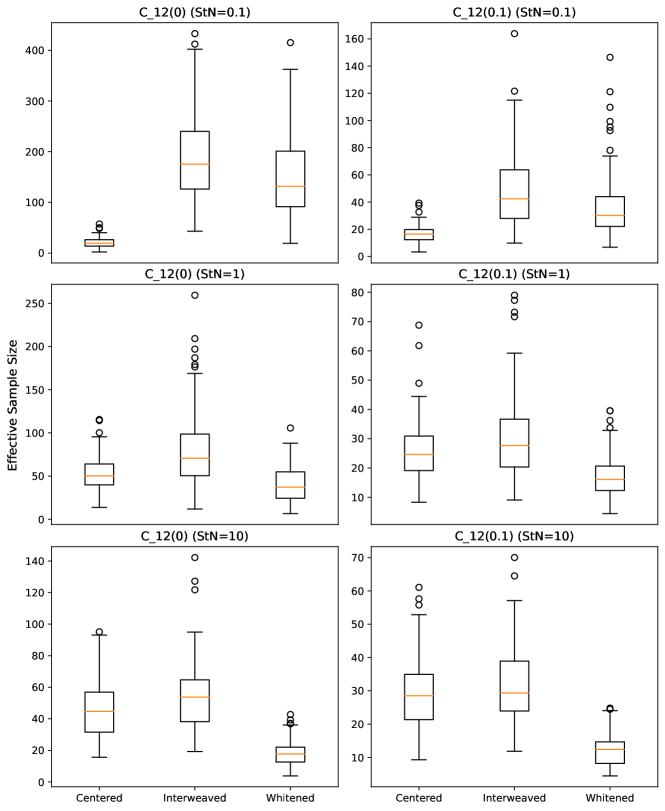
Figure 3: Results of the simulation study described in Section 4.1. Each boxplot contains 100 samples obtained by conducting inference on a new set of observations each time. The effective sample size is calculated for the two Markov chains of length $1000$ corresponding to quantities of interest $C_{12}(0)$ and $C_{12}(0.1)$. The average computing time for the centered, interweaved and whitened algorithms were respectively 33.46, 33.60 and 31.77 seconds.

As expected, the whitened (resp. centered) approach performs poorly when the StN ratio is low (resp. high). The interweaving approach seems to always perform at least slightly better than the most suitable of the other two methods. In practice, we do not know in advance how process level and observational variances compare. Interweaving, as was the objective in its conceptualization (Yu and Meng, 2011), can benefit from the advantages of both worlds, eliminating the need to decide upon an appropriate parametrization.

It is important to emphasize that interweaving samples come at no added computational cost. For all practical purposes, computing time is identical across the three methods (about 30 seconds per chain of length 2000). This is because the computation is dominated by steps 1. and 4. of Algorithm 1 which require respectively ${\mathcal{O}}(p^{2}n^{2})$ (see Appendix E) and ${\mathcal{O}}(pn^{3})$ floating point operations (flops) (inverse and determinant of the $n\times n$ matrices $\boldsymbol{\mathrm{R}}_{j},j=1,\dots,p$). In the vectorized interpretation of the LMC, updating the matrix $\boldsymbol{\mathrm{A}}$ in the centered parametrization would involve computing the inverse and determinant of the $np\times np$ covariance matrix $\sum_{j=1}^{p}\boldsymbol{\mathrm{R}}_{j}\otimes\boldsymbol{\mathrm{a}}_{j}\boldsymbol{\mathrm{a}}_{j}^{\top}$.

A consequence of Proposition 1 is that computations on the coregionalization matrix $\boldsymbol{\mathrm{A}}$ and the spatial correlation matrices $\boldsymbol{\mathrm{R}}_{1},\dots,\boldsymbol{\mathrm{R}}_{p}$ are disentangled when evaluating the likelihood. Updates to $\boldsymbol{\mathrm{A}}$ are negligible when compared to updates of spatial ranges $\varphi_{1},\dots,\varphi_{p}$. Nevertheless, there are $p^{2}$ coregionalization parameters compared to $p$ spatial parameters, hence being able to use more sophisticated samplers on $\boldsymbol{\mathrm{A}}$ (at no additional cost) improves the convergence rate of the MCMC algorithm.

5 Sparse Approach

As a function of dimensionality, the LMC introduces $p^{2}$ parameters. It makes for a model that is not very parsimonious and this might cause overfitting (in the sense of deteriorating predictions at out-of-sample locations) in cases where $p$ is moderately large. There could also exist independencies among the processes; it would perhaps be expected in high dimensional settings. We address those issues by designing a prior that puts probability mass on coregionalization matrices $\boldsymbol{\mathrm{A}}$ that have structural zeros. We introduce the concept of a mask $\boldsymbol{\mathrm{M}}$ which is a binary matrix of the same size as $\boldsymbol{\mathrm{A}}$. The true coregionalization matrix is then the element-wise (Hadamard) product $\boldsymbol{\mathrm{A}}\circ\boldsymbol{\mathrm{M}}$. This matrix still needs to be of full rank such that none of the $p$ processes end up being deterministic linear combinations of the others.

The triangular specification of the LMC discussed in section 3.1 provides an example of a coregionalization matrix with structural zeros (everywhere over the main diagonal in this case). We argued that a lower triangular $\boldsymbol{\mathrm{A}}$ is a model hypothesis that is hard to justify. In comparison, our sparse approach reduces the dimensionality of the parameter space by learning the structure of $\boldsymbol{\mathrm{A}}$ in a principled and data-driven approach.

Same as before, we put i.i.d. normal priors on the elements of, $\boldsymbol{\mathrm{A}}$ which guarantees that $\mathrm{det}(\boldsymbol{\mathrm{A}})\neq 0$ with probability 1. However, this might not hold when setting some elements to zero. For example, setting an entire row or column of $\boldsymbol{\mathrm{M}}$ to zero will always lead to $\boldsymbol{\mathrm{A}}\circ\boldsymbol{\mathrm{M}}$ being singular. For any given binary matrix $\boldsymbol{\mathrm{M}}$ and assuming we assign a distribution to the elements of $\boldsymbol{\mathrm{A}}$ that is absolutely continuous with respect to the $p^{2}$-dimensional Lebesgue measure, we have that $P(\mathrm{det}(\boldsymbol{\mathrm{A}}\circ\boldsymbol{\mathrm{M}})=0)$ is either 0 or 1. We detail below the process by which one can verify if a model, defined by the binary masking matrix $\boldsymbol{\mathrm{M}}$, is admissible in the sense that the matrix $\boldsymbol{\mathrm{A}}\circ\boldsymbol{\mathrm{M}}$ will be of full rank with probability 1.

We start with the Laplace expansion along the $i^{\text{th}}$ line of the determinant

$$\mathrm{det}(\boldsymbol{\mathrm{A}}\circ\boldsymbol{\mathrm{M}})=\sum_{j=1}^{p}a_{ij}m_{ij}C_{ij}$$ (8)

where $C_{ij}$ is the $(i,j)$ cofactor: the determinant of the matrix obtained by removing the $i^{\text{th}}$ line and $j^{\text{th}}$ column of $\boldsymbol{\mathrm{A}}\circ\boldsymbol{\mathrm{M}}$ multiplied by $(-1)^{i+j}$. Equation (8) will be equal to 0 if and only if every summand is identically 0.

The determinant can be expanded from any row or column. If any of those consists entirely of 0s, then expression (8) will be equal to 0 with probability 1. This will be a stopping condition for the recursive algorithm designed to evaluate the admissibility of a model $\boldsymbol{\mathrm{M}}$. The other stopping state is when there are globally less than $p$ zeros; in that case, expression (8) is almost surely not equal to 0. Indeed, this is trivially true for $p=1$ and can be shown to be true for any $p$ by induction using the Laplace expansion.

Equation (8) allows us to transform a statement about a $p\times p$ matrix into verifying the same condition on smaller $(p-1)\times(p-1)$ matrices. The determinant will be identically zero if and only if all the determinants of the smaller matrices are identically 0 (those corresponding to the non-zero entries of the line or column we chose to expand from). A good strategy is thus to always expand the determinant by the row or column that contains the most 0s to minimize the number of recursive calls.

This allows us to formulate a hierarchical prior where the model $\boldsymbol{\mathrm{M}}$ is selected at the first stage, regardless of $\boldsymbol{\mathrm{A}}$, among admissible ones. The respective entries of the coregionalization matrix are assigned at the later stage. The prior on the masking matrix is assumed to take the form

$$p(\boldsymbol{\mathrm{M}})\propto\pi^{\sum m_{ij}}(1-\pi)^{p^{2}-\sum m_{ij}},$$

where $\sum m_{ij}$ is the number of 1s contained in $\boldsymbol{\mathrm{M}}$ and $\pi\in[0,1]$ is a hyperparameter controlling prior belief on the degree of sparsity. It is essentially the prior probability for an entry of $\boldsymbol{\mathrm{A}}$ to be non-zero, subject to the restrictions described above.

We use the framework of reversible jump Markov chain Monte-Carlo (Green, 1995) to conceive proposals to the coregionalization matrix $\boldsymbol{\mathrm{A}}$ that allow trans-dimensional updates. At every step, we either propose to replace a non-zero entry with a 0 or to assign a new value to a previously null entry. We chain $p$ of those proposals at each iteration of the Markov chain. Everything else is just as in Algorithm 1. Again, the computational overhead is negligible in the context where we also estimate range parameters $\varphi_{j=1}^{p}$, the updates to which are orders of magnitude more costly. In the next section, we conduct an experiment designed to evaluate the effect on predictive accuracy of our sparsity-inducing approach.

5.1 Simulation Study

We start with $n=100$ irregularly spaced locations on the unit square where we instantiate our multivariate process. We then interpolate the random fields to a regular $10\times 10$ grid covering the domain and compare it with the held-out ground truth. We use the root mean squared error as our evaluation metric. The model is simulated according to the LMC for each of two examples.

In the first, the coregionalization matrix is full in the sense that it has no structural zeros. All processes are interdependent. In the second example, every entry of $\boldsymbol{\mathrm{A}}$ is zero except the main diagonal hence the $p$ resulting processes are mutually independent. In both cases, each line of the matrix $\boldsymbol{\mathrm{A}}$ is scaled so that each process has unit marginal variance. We add an observational noise of variance 0.25 to the $p$ components at each location. The underlying LMC is thus nowhere observed directly. For the range parameters $\varphi_{j},j=1,\dots,p$, we split the $[5,25]$ interval with equal gaps on the logarithmic scale so for example we use (5, 7.48, 11.18, 16.72, 25) when $p=5$. This is to ensure the $p$ underlying processes are as distinguishable as possible while having range inside the [3,30] support. For each of $p=2,3,4,5$, we simulate 100 LMC realizations. We then run the MCMC algorithm for 2000 iterations on each of them, keeping only the last 1000. We use $\pi=1/p$ throughout as our prior belief on the degree of sparsity. The results of our experiments for the full and diagonal examples are respectively showcased in Figures 4 and 5.

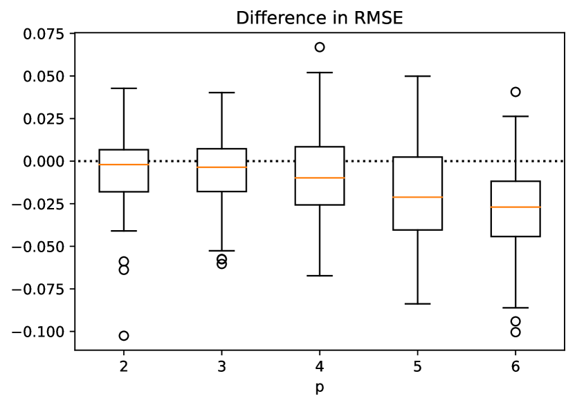
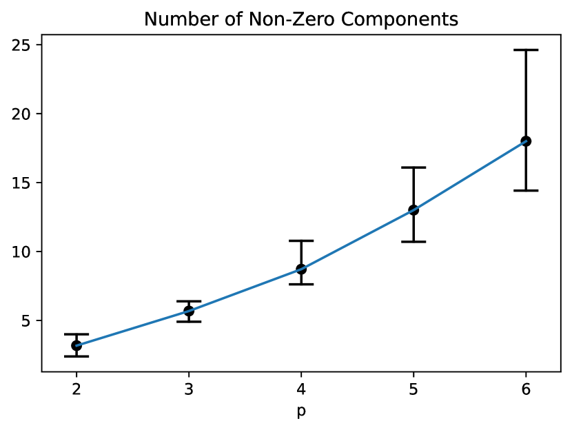
Figure 4: Comparison of our sparse method with the standard approach for the case of a full (no zeros) coregionalization matrix. On the left, the difference (sparse minus standard) in RMSE computed on each realization. On the right, the mean number of non-zero components in the matrix $\boldsymbol{\mathrm{A}}$ along with 90% credible intervals. The distributions illustrated are across the 100 simulated LMC realizations.

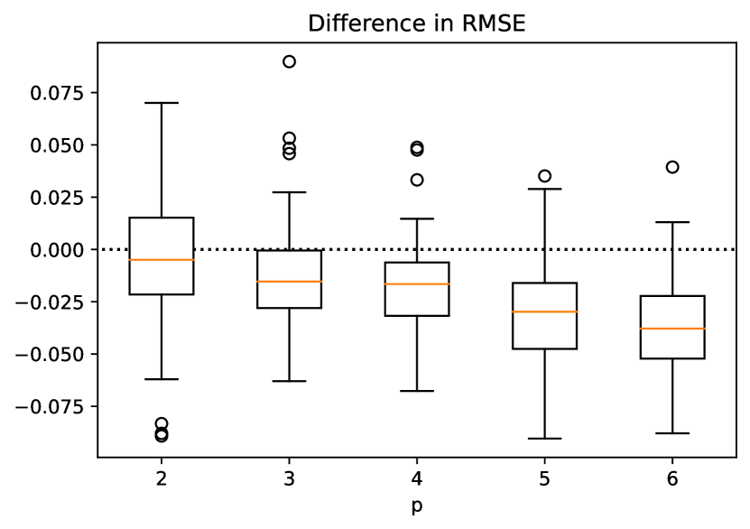
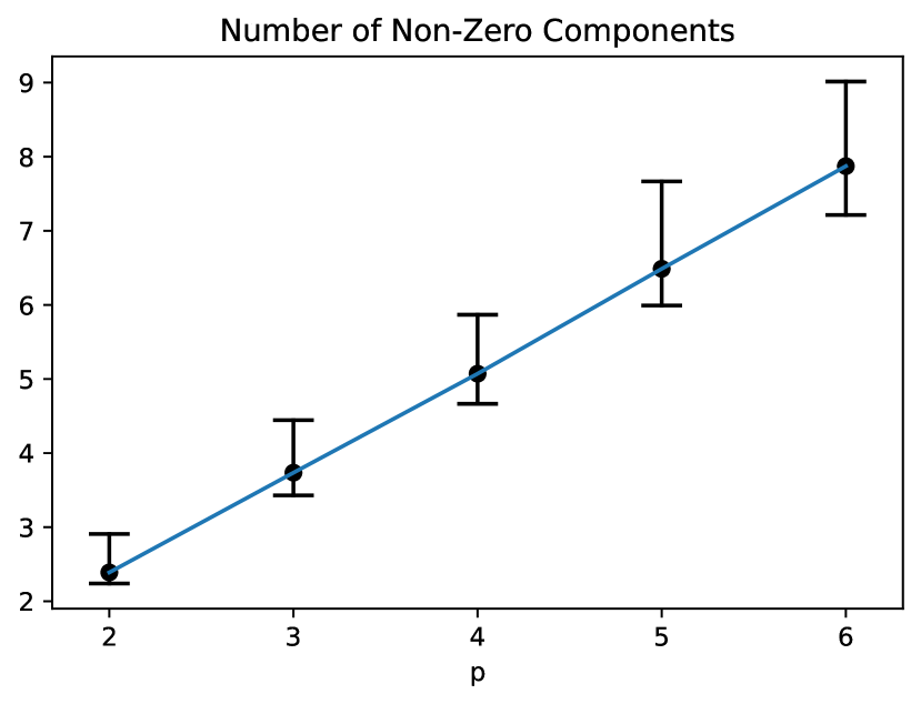
Figure 5: Comparison of our sparse method with the standard approach for the case of a diagonal coregionalization matrix (independent components). On the left, the difference (sparse minus standard) in RMSE computed on each realization. On the right, the mean number of non-zero components in the matrix $\boldsymbol{\mathrm{A}}$ along with 90% credible intervals. The distributions illustrated are across the 100 simulated LMC realizations.

In lower dimension $p$, there is little difference in using either of the two estimation methods. However, as dimensions increase, predictions from the sparse model appear more accurate than those under the standard approach with no structural zeros. This is certainly expected for the diagonal example as there are only $p$ non-zero entries in the coregionalization matrix. It is perhaps more remarkable for the full $\boldsymbol{\mathrm{A}}$ case where a misspecified but sparser model better generalizes to out-of-sample predictions. This is because the number $p^{2}$ of coregionalization parameters to estimate rapidly becomes unwieldy when compared to the number of observed locations. Our sparse approach facilitates the use of the LMC in such scenarios. We can also see on the right side of Figures 4 and 5 that our method indeed manages to curb the growth of parameters especially in the diagonal case where we observe a seemingly linear relation.

			$p$
Method	2	3	4	5	6
Sparse	19.556	29.832	41.604	56.511	74.907
Standard	19.165	29.265	40.523	54.902	72.660

Table 1: Mean time (in seconds) elapsed per model fitting for the different scenarios.

In Table 1, we compare the computing time of the sparse and standard specifications. Our approach adds very little computing time when compared to the traditional LMC. As was the case for the interweaving algorithm, this is because recomputing the likelihood upon a modification of the coregionalization matrix $\boldsymbol{\mathrm{A}}$ is negligible in terms of computations when compared to an update of the spatial range parameters. In the next section, we apply our sparse methodology to a real dataset to showcase the inferential properties of our model.

5.2 Analysis of California Air Data

In this section, we analyze a data set consisting of measurements in the concentration of four pollutants: carbon monoxide (CO), nitric oxide (NO), nitrogen dioxide (NO₂) and ozone (O₃). There are no covariates included. Our interest is mainly in inferring the cross-covariance structure. We use the reversible jump sampler for the coregionalization matrix $\boldsymbol{\mathrm{A}}$. This will help us identify potential independencies among the measured quantities.

We analyze the data on the log scale to achieve approximate normality. Those quantities are measured at monitoring sites spread across the state of California. Those locations, projected to the unit square, are illustrated in Figure 6. The data is available publicly on the California Air Resources Board website. We chose the date of 26/04/2002 as it had a high number of sites where all 4 components were measured (83 in total).

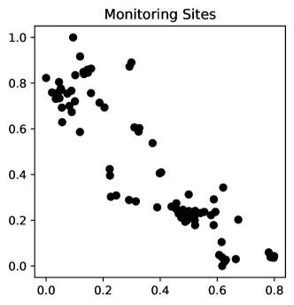
Figure 6: Projected locations of the 83 monitoring stations used in the analysis of the California air data.

Data from this database was also analyzed in Schmidt and Gelfand (2003) although in the summer rather than the spring and without the ozone component. Nevertheless, the resulting inference we present here, while not identical, seems to be at least coherent with their findings in terms of the magnitude of correlations among the three components CO, NO and NO₂.

We again assign independent Gaussian priors to the non-zero components of $\boldsymbol{\mathrm{A}}$. The range components $\varphi_{j=1}^{p}$ are constrained to the uniform [3,30] distribution, a priori. The observational noise variance parameters are given inverse gamma prior distributions. The log concentrations of each of the four pollutants do not appear to share a common mean hence we add a component-specific mean structure to the LMC. The $p$-dimensional mean vector $\boldsymbol{\mathrm{\mu}}$ is assigned a Gaussian distribution with diagonal covariance to obtain conjugate normal full conditional updates. Finally, we use $1/p=0.25$ for the hyperparameter $\pi$ that controls the degree of sparsity. We run the MCMC algorithm for 150,000 iterations, discarding the first 50,000 as burn-in.

The posterior samples of the covariance and correlation matrices are summarized in Figure 7. We can see some of the credible intervals have boundaries that are exactly 0. This is a consequence of assigning prior probability mass at 0 for the elements of $\boldsymbol{\mathrm{A}}$. Another interesting component of our sparsity-inducing approach to the LMC is that we can evaluate the posterior probability of 2 processes to be independent. Those probabilities are illustrated in Figure 8 along with the distribution of non-zero elements in the matrix $\boldsymbol{\mathrm{A}}$. It seems to potentially indicate that the CO pollutant could be uncorrelated with the other 3. Further evidence would be needed before reaching this conclusion, but this is not the object of this paper. Modeling pairwise dependencies among the other components seems to be worth it since they have 0 (or very small) probability of being independent. In Figure 9, we show the posterior probabilities of independence in an alternate scenario where we simulate an independent fifth component (D). We can see that our model appropriately captures this independency. Finally, we illustrate the cross-covariance among pollutants as functions of distance in Figure 10. We notice the strong positive correlation between the NO and NO₂ components. Also, the ozone pollutant seems to be negatively correlated with the other 3.

CO	NO	NO2	O3
0.18 (0.01;0.62)
0.21 (0.00;0.57)	0.79 (0.46;1.42)
0.13 (0.00;0.41)	0.56 (0.33;1.06)	0.58 (0.32;1.05)
-0.04 (-0.12;0.00)	-0.16 (-0.32;-0.09)	-0.13 (-0.26;-0.07)	0.04 (0.02;0.09)

(a) Covariance Matrix

CO	NO	NO2	O3
1.00 (1.00;1.00)
0.58 (0.00;0.89)	1.00 (1.00;1.00)
0.45 (0.00;0.85)	0.85 (0.69;0.96)	1.00 (1.00;1.00)
-0.56 (-0.89;0.00)	-0.95 (-1.00;-0.75)	-0.88 (-0.99;-0.67)	1.00 (1.00;1.00)

(b) Correlation Matrix

Figure 7: Posterior median of the marginal (at each location) covariance and correlation matrices along with the 0.05 and 0.95 quantiles in parenthesis. Left to right (top to bottom): CO, NO, NO₂,O₃.

	CO	NO	NO2	O3
CO	0.0000
NO	0.1787	0.0000
NO2	0.3190	0.0000	0.0000
O3	0.3229	0.0007	0.0005	0.0000

(a) Pairwise Probability of Independence

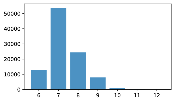
(b) Number of Non-Zero Elements of $\boldsymbol{\mathrm{A}}$

Figure 8:

	CO	NO	NO2	O3	D
CO	0.0000	0.1992	0.3852	0.3824	0.7513
NO	0.1992	0.0000	0.0000	0.0000	0.8077
NO2	0.3852	0.0000	0.0000	0.0000	0.7184
O3	0.3824	0.0000	0.0000	0.0000	0.8450
D	0.7513	0.8077	0.7184	0.8450	0.0000

Figure 9: Pairwise probability of independence with the component D being an independent Gaussian process with mean -3.92, unit variance and range parameter equal to 10.

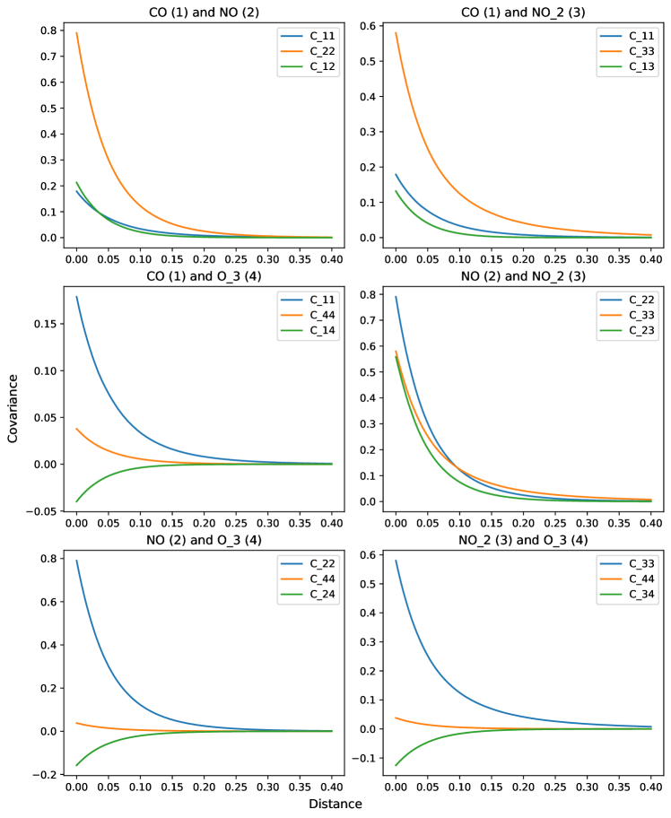
Figure 10: Pointwise posterior median of the cross-covariance functions.

6 Discussion

We revisited the LMC as a constructive approach to specifying cross-covariance functions, deriving some important characteristics in the process. Starting with the separable specification of the LMC and its link with the matrix normal distribution, we were able to make an analogous connection between the more general LMC and a new kind of Gaussian distribution for matrices. Doing so exposed a covariance structure that can be exploited to obtain likelihood evaluations in a number of operations that is linear in the dimensionality $p$. Computational scalability might just be the strongest suit of the LMC, a fact that has not been taken advantage of in the literature about multivariate Gaussian processes. Since this is not an approximation, there are only benefits to using the formulation we describe in Section 3.

Beyond the plain computational speedups, there are other advantages to the matrix normal representation of the LMC. Foremost, the coregionalization matrix $\boldsymbol{\mathrm{A}}$ is not entangled with the spatial correlation matrices $\boldsymbol{\mathrm{R}}_{1},\dots,\boldsymbol{\mathrm{R}}_{p}$ in the likelihood. In particular, an update to $\boldsymbol{\mathrm{A}}$ does not require computing the inverse and determinant of any $np\times np$ sized matrix. Even though it is generally small in comparison with the spatial correlation matrices, the matrix $\boldsymbol{\mathrm{A}}$ contains more parameters and can become difficult to estimate whenever $p$ is moderately large. However, updates now come cheap so we can incorporate more involved samplers without much of an effect on the total computing time.

We designed and evaluated two of those alternatives. The first is intended to alleviate the auto-correlation in the Markov chain of posterior samples for the elements of $\boldsymbol{\mathrm{A}}$. This strong dependence can often plague Gibbs samplers where blocks of parameters are updated in turn. We outlined an interweaving strategy that updates the coregionalization matrix twice based correspondingly on a centered and whitened parametrization of the underlying random fields. The second sampler aims to reduce the dimensionality of the parameter space by introducing structural zeros in $\boldsymbol{\mathrm{A}}$. This type of regularization can benefit the accuracy of predictions as was observed on out-of-sample data in Section 5. Moreover, our sparse approach to the LMC can offer interesting insights by discovering potential independencies among the $p$ modeled components.

In terms of future developments and applications, we can think of a few. First, since the computational structure is preserved under conditioning, we would like to see it exploited and fully integrated into the framework of Vecchia approximations like the nearest neighbor approach. This would in principle be a straightforward application of propositions 1 and 2. It would form a class of highly scalable (as a function of both $n$ and $p$) multivariate Gaussian models. Finally, we used the flexibility of the matrix normal formulation to implement two alternative MCMC algorithms. We believe researchers can get even more creative and design samplers that facilitate estimation in particular contexts and applications.

Appendix A Proof of Proposition 1

We can think of a vectorized form $\boldsymbol{\mathrm{w}}^{\prime}=(\boldsymbol{\mathrm{w}}_{1},\boldsymbol{\mathrm{w}}_{2},\dots,\boldsymbol{\mathrm{w}}_{p})^{\top}$ for the base processes where we stack the $p$ $n$-dimensional processes instead of ordering by locations. This is how it is presented in Jin et al. [2007] in the context of multivariate conditional auto-regressive models rather than continuously indexed spatial data. The authors get fairly far along the argument we use here.

Since we start with independent processes, the $np\times np$ covariance matrix of $\boldsymbol{\mathrm{w}}^{\prime}$ is block diagonal with blocks consisting of the $n\times n$ correlation matrices $\boldsymbol{\mathrm{R}}_{1},\dots,\boldsymbol{\mathrm{R}}_{p}$. In the usual representation (ordered by locations), we would consider the $np$-dimensional vector $\boldsymbol{\mathrm{w}}=(\boldsymbol{\mathrm{w}}(\boldsymbol{\mathrm{s}}_{1})^{\top},\boldsymbol{\mathrm{w}}(\boldsymbol{\mathrm{s}}_{2})^{\top},\dots,\boldsymbol{\mathrm{w}}(\boldsymbol{\mathrm{s}}_{n})^{\top})^{\top}$. Of course, $\boldsymbol{\mathrm{w}}$ is obtained by a permutation of the elements of $\boldsymbol{\mathrm{w}}^{\prime}$ so there exists a permutation matrix $\boldsymbol{\mathrm{P}}$ for which $\boldsymbol{\mathrm{w}}=\boldsymbol{\mathrm{P}}\boldsymbol{\mathrm{w}}^{\prime}$ and $\mathrm{Var}(\boldsymbol{\mathrm{w}})=\boldsymbol{\mathrm{P}}\mathrm{diag}\{\boldsymbol{\mathrm{R}}_{1},\dots,\boldsymbol{\mathrm{R}}_{p}\}\boldsymbol{\mathrm{P}}^{\top}$.

The multivariate process $\boldsymbol{\mathrm{v}}=(\boldsymbol{\mathrm{v}}(\boldsymbol{\mathrm{s}}_{1})^{\top},\boldsymbol{\mathrm{v}}(\boldsymbol{\mathrm{s}}_{2})^{\top},\dots,\boldsymbol{\mathrm{v}}(\boldsymbol{\mathrm{s}}_{n})^{\top})^{\top}$ with cross-dependence is obtained from $\boldsymbol{\mathrm{w}}$ by transforming each location as $\boldsymbol{\mathrm{v}}(\boldsymbol{\mathrm{s}})=\boldsymbol{\mathrm{A}}\boldsymbol{\mathrm{w}}(\boldsymbol{\mathrm{s}})$. For the vectorized forms, this means that $\boldsymbol{\mathrm{v}}$ is obtained by multiplying a block diagonal matrix consisting of $n$ $\boldsymbol{\mathrm{A}}$ matrices along the diagonal with $\boldsymbol{\mathrm{w}}$. Putting all the above together, we can write the covariance of the vectorized $\boldsymbol{\mathrm{v}}$ as

$$\mathrm{Var}(\boldsymbol{\mathrm{v}})=\left(\begin{matrix}\boldsymbol{\mathrm{A}}&\boldsymbol{\mathrm{0}}&\dots&\boldsymbol{\mathrm{0}}\\ \boldsymbol{\mathrm{0}}&\boldsymbol{\mathrm{A}}&\dots&\boldsymbol{\mathrm{0}}\\ \vdots&\vdots&\ddots&\vdots\\ \boldsymbol{\mathrm{0}}&\boldsymbol{\mathrm{0}}&\dots&\boldsymbol{\mathrm{A}}\end{matrix}\right)\boldsymbol{\mathrm{P}}\left(\begin{matrix}\boldsymbol{\mathrm{R}}_{1}&\boldsymbol{\mathrm{0}}&\dots&\boldsymbol{\mathrm{0}}\\ \boldsymbol{\mathrm{0}}&\boldsymbol{\mathrm{R}}_{2}&\dots&\boldsymbol{\mathrm{0}}\\ \vdots&\vdots&\ddots&\vdots\\ \boldsymbol{\mathrm{0}}&\boldsymbol{\mathrm{0}}&\dots&\boldsymbol{\mathrm{R}}_{p}\end{matrix}\right)\boldsymbol{\mathrm{P}}^{\top}\left(\begin{matrix}\boldsymbol{\mathrm{A}}^{\top}&\boldsymbol{\mathrm{0}}&\dots&\boldsymbol{\mathrm{0}}\\ \boldsymbol{\mathrm{0}}&\boldsymbol{\mathrm{A}}^{\top}&\dots&\boldsymbol{\mathrm{0}}\\ \vdots&\vdots&\ddots&\vdots\\ \boldsymbol{\mathrm{0}}&\boldsymbol{\mathrm{0}}&\dots&\boldsymbol{\mathrm{A}}^{\top}\end{matrix}\right).$$ (9)

Lemma 1.

The inverse for the covariance matrix of the vectorized form $(\boldsymbol{\mathrm{v}}(\boldsymbol{\mathrm{s}}_{1})^{\top},\dots,\boldsymbol{\mathrm{v}}(\boldsymbol{\mathrm{s}}_{n})^{\top})^{\top}$ of the LMC can be computed as

$$\left(\sum_{j=1}^{p}\boldsymbol{\mathrm{R}}_{j}\otimes\boldsymbol{\mathrm{a}}_{j}\boldsymbol{\mathrm{a}}_{j}^{\top}\right)^{-1}=\sum_{j=1}^{p}\boldsymbol{\mathrm{R}}_{j}^{-1}\otimes\boldsymbol{\mathrm{a}}_{j}^{-\top}\boldsymbol{\mathrm{a}}_{j}^{-1},$$

where $\boldsymbol{\mathrm{a}}_{j}^{-1}$ is the $j^{\text{th}}$ line of the inverse matrix $\boldsymbol{\mathrm{A}}^{-1}$.

Proof.

This can be shown by direct verification. Alternatively, from equation (9) we can guess the inverse

$$\left(\begin{matrix}\boldsymbol{\mathrm{A}}^{-\top}&\boldsymbol{\mathrm{0}}&\dots&\boldsymbol{\mathrm{0}}\\ \boldsymbol{\mathrm{0}}&\boldsymbol{\mathrm{A}}^{-\top}&\dots&\boldsymbol{\mathrm{0}}\\ \vdots&\vdots&\ddots&\vdots\\ \boldsymbol{\mathrm{0}}&\boldsymbol{\mathrm{0}}&\dots&\boldsymbol{\mathrm{A}}^{-\top}\end{matrix}\right)\boldsymbol{\mathrm{P}}\left(\begin{matrix}\boldsymbol{\mathrm{R}}_{1}^{-1}&\boldsymbol{\mathrm{0}}&\dots&\boldsymbol{\mathrm{0}}\\ \boldsymbol{\mathrm{0}}&\boldsymbol{\mathrm{R}}_{2}^{-1}&\dots&\boldsymbol{\mathrm{0}}\\ \vdots&\vdots&\ddots&\vdots\\ \boldsymbol{\mathrm{0}}&\boldsymbol{\mathrm{0}}&\dots&\boldsymbol{\mathrm{R}}_{p}^{-1}\end{matrix}\right)\boldsymbol{\mathrm{P}}^{\top}\left(\begin{matrix}\boldsymbol{\mathrm{A}}^{-1}&\boldsymbol{\mathrm{0}}&\dots&\boldsymbol{\mathrm{0}}\\ \boldsymbol{\mathrm{0}}&\boldsymbol{\mathrm{A}}^{-1}&\dots&\boldsymbol{\mathrm{0}}\\ \vdots&\vdots&\ddots&\vdots\\ \boldsymbol{\mathrm{0}}&\boldsymbol{\mathrm{0}}&\dots&\boldsymbol{\mathrm{A}}^{-1}\end{matrix}\right)$$

which is exactly the claimed solution. ∎

Lemma 2.

The determinant for the covariance matrix of the vectorized form $(\boldsymbol{\mathrm{v}}(\boldsymbol{\mathrm{s}}_{1})^{\top},\dots,\boldsymbol{\mathrm{v}}(\boldsymbol{\mathrm{s}}_{n})^{\top})^{\top}$ of the LMC can be computed as

$$\mathrm{det}\left(\sum_{j=1}^{p}\boldsymbol{\mathrm{R}}_{j}\otimes\boldsymbol{\mathrm{a}}_{j}\boldsymbol{\mathrm{a}}_{j}^{\top}\right)=\mathrm{det}(\boldsymbol{\mathrm{A}})^{2n}\prod_{j=1}^{p}\mathrm{det}(\boldsymbol{\mathrm{R}}_{j}).$$

Proof.

Evident from equation (9) since the determinant of the permutation matrix $\boldsymbol{\mathrm{P}}$ is either 1 or -1. ∎

The final step to prove Proposition 1 is to express the $p$ quadratic products $\boldsymbol{\mathrm{v}}^{\top}\left(\boldsymbol{\mathrm{R}}_{j}^{-1}\otimes\boldsymbol{\mathrm{a}}_{j}^{-\top}\boldsymbol{\mathrm{a}}_{j}^{-1}\right)\boldsymbol{\mathrm{v}}$ using the matrix form $\boldsymbol{\mathrm{V}}$ of the LMC. The $np$-vector $\boldsymbol{\mathrm{v}}$ is obtained by stacking the columns of $\boldsymbol{\mathrm{V}}$ hence we write $\boldsymbol{\mathrm{v}}=\mathrm{vec}(\boldsymbol{\mathrm{V}})$. We can then use the well known identities $(\boldsymbol{\mathrm{C}}^{\top}\otimes\boldsymbol{\mathrm{A}})\mathrm{vec}(\boldsymbol{\mathrm{B}})=\mathrm{vec}(\boldsymbol{\mathrm{A}}\boldsymbol{\mathrm{B}}\boldsymbol{\mathrm{C}})$ and $\mathrm{vec}(\boldsymbol{\mathrm{A}})^{\top}\mathrm{vec}(\boldsymbol{\mathrm{B}})=\mathrm{tr}(\boldsymbol{\mathrm{A}}^{\top}\boldsymbol{\mathrm{B}})$ in this order to obtain

$$\mathrm{vec}(\boldsymbol{\mathrm{V}})^{\top}\left(\boldsymbol{\mathrm{R}}_{j}^{-1}\otimes\boldsymbol{\mathrm{a}}_{j}^{-\top}\boldsymbol{\mathrm{a}}_{j}^{-1}\right)\mathrm{vec}(\boldsymbol{\mathrm{V}})=\mathrm{tr}(\boldsymbol{\mathrm{V}}^{\top}\boldsymbol{\mathrm{a}}_{j}^{-\top}\boldsymbol{\mathrm{a}}_{j}^{-1}\boldsymbol{\mathrm{V}}\boldsymbol{\mathrm{R}}_{j}^{-1})$$

and use the cyclic property of the trace to express it as the scalar $\boldsymbol{\mathrm{a}}_{j}^{-1}\boldsymbol{\mathrm{V}}\boldsymbol{\mathrm{R}}_{j}^{-1}\boldsymbol{\mathrm{V}}^{\top}\boldsymbol{\mathrm{a}}_{j}^{-\top}$.

The argument can be recycled for models where the coregionalization matrix varies over locations. Such is the case for the non-stationary LMC proposed by Gelfand et al. [2004] where the matrix $\boldsymbol{\mathrm{A}}$ varies smoothly across space. In that case, we can index the coregionalization matrix $\boldsymbol{\mathrm{A}}_{i}$ with location numbers $i=1,2,\dots,n$. Those would appear in sequence in place of the singular $\boldsymbol{\mathrm{A}}$ on the diagonal in equation (9). This implies that the inverse and determinant of the covariance matrix implied by the nonstationary version of the LMC can also be computed from those of the individual matrices; this time the $n$ $p\times p$ coregionalization matrices $\boldsymbol{\mathrm{A}}_{i}$ and the $p$ $n\times n$ spatial correlation matrices $\boldsymbol{\mathrm{R}}_{j}$.

Appendix B Identifiability

In the case where exponential correlation functions $\rho(\boldsymbol{\mathrm{s}},\boldsymbol{\mathrm{t}})=\exp(-\varphi_{j}|\boldsymbol{\mathrm{s}}-\boldsymbol{\mathrm{t}}|)$ are assigned to the base processes $w_{j}(\cdot),j=1,\dots,p$, we will show that one can identify both the full rank coregionalization matrix $\boldsymbol{\mathrm{A}}$ along with range parameters $\varphi_{1},\dots,\varphi_{p}$. We will assume without loss of generality that the range parameters are in increasing order such that $\varphi_{1}<\dots<\varphi_{p}$. To be clear, we mean that provided there is a sufficient number $n$ of points (to be clarified below), parameters $\boldsymbol{\mathrm{A}},\varphi_{j=1}^{p}$ and $\boldsymbol{\mathrm{B}},\psi_{j=1}^{p}$ will lead to the same model if and only if $\varphi_{j}=\psi_{j}$ for all $j$ and $\boldsymbol{\mathrm{A}}=\boldsymbol{\mathrm{B}}$ up to column sign switches. This is unlike the separable case ($\varphi_{1}=\varphi_{2}=\dots=\varphi_{p}$) where the model is a function of the product $\boldsymbol{\mathrm{A}}\boldsymbol{\mathrm{A}}^{\top}$. There exists an infinity of equivalent such factorizations. Standard examples include the lower triangular Cholesky decomposition or the positive definite square root.

To establish this result, we first look at the cross-covariance function of components $i$ and $j$ evaluated at distance $d$:

$$C_{ij}(d)=\sum_{k=1}^{p}a_{ik}a_{jk}\exp(-\varphi_{k}d).$$

We postulate for a contradiction that another set of parameters $\boldsymbol{\mathrm{B}},\psi_{j=1}^{p}$ leads to the same model. This leads to equations

$$f_{ij}(d):=\sum_{k=1}^{p}a_{ik}a_{jk}\exp(-\varphi_{k}d)-\sum_{\ell=1}^{p}b_{i\ell}b_{j\ell}\exp(-\psi_{\ell}d)=0,\qquad i,j=1,\dots,p.$$ (10)

According to Laguerre’s generalization [Laguerre, 1884] of Descartes’ rule of signs, each $f_{ij}$ above either has at most $2p-1$ positive roots or is identically 0 everywhere. We debunk the latter first.

For $f_{ij}$ to be zero everywhere, it needs to be the case that $\varphi_{k}=\psi_{k}$ for all $k$. Otherwise, if there is a $\varphi_{k}$ that is not equal to any of the alternative range parameters, then it means in particular that the coefficients $a_{ik}^{2}=0$ for each $i=1,\dots,p$. This signifies a column of 0s in $\boldsymbol{\mathrm{A}}$ which is not allowed ($\boldsymbol{\mathrm{A}}$ is of full rank). So we can assume $\varphi_{k}=\psi_{k},k=1,\dots,p$ since both sets are ordered.

Consequently, for the $f_{ii}(d)$ to be 0 everywhere we now need the coefficients $a_{ik}^{2}-b_{ik}^{2}$ to be equal to zero for all $i,k=1,\dots,p$; every entry of $\boldsymbol{\mathrm{B}}$ is equal to the corresponding entry in $\boldsymbol{\mathrm{A}}$ up to a change of sign. We also need $a_{ik}a_{jk}-b_{ik}b_{jk}=0$ for every $j=1,\dots,p$ so if an entry $a_{ik}=-b_{ik}$, then the whole column needs to be sign flipped. For all $f_{ij}(d)$ to be zero everywhere, the range parameters need to be the same, and $\boldsymbol{\mathrm{A}}$ and $\boldsymbol{\mathrm{B}}$ are equal up to column sign changes.

However, it may be the case that the $2p-1$ possible roots of the $f_{ij}$ functions are enough to obtain 2 equivalent models at least at the locations observed. However, if there are more than $2p-1$ distinct distances among the points observed, then there wouldn’t be enough roots for the 2 models to agree on all of those. For example, let’s say the multivariate process $\boldsymbol{\mathrm{v}}(\boldsymbol{\mathrm{s}})$ is observed at locations contained in the plane $\mathds{R}^{2}$. If there are $n$ such points, then we know from the Erdös distinct distances problem [Erdös, 1946] that there are at the very least $\sqrt{n-3/4}-1/2$ different pairwise distances. It means that if there is a minimum of $(2p-1/2)^{2}+3/4$ points, then the LMC is guaranteed to be identifiable in this context. Most often, points come in no regular pattern and hence present $n(n-1)/2$ distinct distances (as many as there are pairs of points) and such a number usually exceeds $2p-1$ by a large amount.

Appendix C Cross-Covariance Functions

There is a vast literature on cross-covariance functions for multivariate Gaussian processes. We review some of the modeling advantages and drawbacks, specifically when compared to the LMC.

In the approach of Apanasovich and Genton [2010] based on latent dimensions, a $p$-variate cross-covariance function is defined from a single univariate one over $\mathds{R}^{d+k}$ ($1\leq k\leq p$) by

$$C_{ij}(\boldsymbol{\mathrm{s}},\boldsymbol{\mathrm{t}})=C\{(\boldsymbol{\mathrm{s}},\boldsymbol{\mathrm{\xi}}_{i}),(\boldsymbol{\mathrm{t}},\boldsymbol{\mathrm{\xi}}_{j})\},\qquad\text{with }\boldsymbol{\mathrm{s}},\boldsymbol{\mathrm{t}}\in\mathds{R}^{d};\boldsymbol{\mathrm{\xi}}_{i},\boldsymbol{\mathrm{\xi}}_{j}\in\mathds{R}^{k}.$$ (11)

The cross-covariance above is valid by construction. The authors use this idea to generalize the class of space-time covariance functions described in Gneiting [2002] to multivariate data. Ignoring the time component for simplicity, the framework described by equation (11) is employed to construct a cross-covariance function of the form

$$C_{ij}(|\boldsymbol{\mathrm{s}}-\boldsymbol{\mathrm{t}}|)=\frac{\sigma^{2}}{|\boldsymbol{\mathrm{\xi}}_{i}-\boldsymbol{\mathrm{\xi}}_{j}|+1}\exp\left(\frac{-\alpha|\boldsymbol{\mathrm{s}}-\boldsymbol{\mathrm{t}}|}{(|\boldsymbol{\mathrm{\xi}}_{i}-\boldsymbol{\mathrm{\xi}}_{j}|+1)^{\beta/2}}\right).$$ (12)

The interesting part of expression (12) is the presence of a single parameter $\beta\in[0,1]$ controlling separability. Another notable fact is how parsimonious model (12) is in terms of parameters. It involves $p$ locations $\boldsymbol{\mathrm{\xi}}_{1},\dots,\boldsymbol{\mathrm{\xi}}_{p}$, each one in $\mathds{R}^{k}$, along with the parameters of the single covariance function over $\mathds{R}^{d+k}$. In comparison, the LMC has $p^{2}$ components in its coregionalization matrix $\boldsymbol{\mathrm{A}}$ plus the individual parameters contained in the $p$ distinct univariate correlation functions $\rho_{j}(\cdot)$. We propose an approach to curb this potential over-parametrization problem in Section 5.

An inconvenience of using (11), or the specific instance (12) of it, is that it leads to identical marginal models for each of the $p$ processes. Perhaps less apparent is the fact that the cross-covariance (for $i\neq j$) functions under (11) are themselves valid univariate covariance functions. For general $d$ and stationary-isotropic covariances that are a function of distance $|\boldsymbol{\mathrm{s}}-\boldsymbol{\mathrm{t}}|$, that restricts cross-covariances to the class of completely monotone functions (see Cressie [1993, Section 2.5.1]). In particular, negative correlation across processes is prohibited at any distance. [Apanasovich and Genton, 2010] propose to circumvent those limitations by using linear combinations of multiple processes, something that is very similar in spirit to what the LMC does.

In terms of univariate correlation functions, there are perhaps none more celebrated than those of the Matérn class [Matérn, 1960] defined by

$$M(\boldsymbol{\mathrm{s}}-\boldsymbol{\mathrm{t}}|\nu,\varphi)=\frac{2^{1-\nu}}{\Gamma(\nu)}(\varphi|\boldsymbol{\mathrm{s}}-\boldsymbol{\mathrm{t}}|)^{\nu}K_{\nu}(\varphi|\boldsymbol{\mathrm{s}}-\boldsymbol{\mathrm{t}}|),$$ (13)

where $K_{\nu}$ is the modified Bessel function and $\varphi$ is a range parameter. Smoothness is handled by $\nu$ in the sense that any stationary random field with correlation function (13) has $\lceil\nu\rceil-1$ differentiable sample paths in the mean-square sense [Guttorp and Gneiting, 2006]. The Matérn class includes the exponential correlation function, among others, as a special case when $\nu=1/2$.

The objective of a multivariate Matérn covariance function is to have Matérn marginal covariances for the $p$ processes while still allowing cross-dependence among them. Gneiting et al. [2010] specified a stationary cross-covariance function of the form,

$$C_{ij}(|\boldsymbol{\mathrm{s}}-\boldsymbol{\mathrm{t}}|)=\sigma_{ij}M(\boldsymbol{\mathrm{s}}-\boldsymbol{\mathrm{t}}|\nu_{ij},\varphi_{ij}),\qquad i,j=1,\dots,p.$$ (14)

Conditions need to be imposed on parameters $\nu_{ij},\varphi_{ij}$ to ensure a positive definite covariance. The authors first propose a parsimonious model obtained by applying the covariance convolution approach of Majumdar and Gelfand [2007] (which is itself a rich conceptual framework for constructing valid multivariate covariance functions). However, this approach imposes strong restrictions on the parameters of (3). It requires every range parameter $\varphi_{ij}$ to have the same value but still allows each process to have its own differentiability parameter $\nu_{ii}>0$.

Gneiting et al. [2010] also described a more general formulation for $p=2$ by establishing a sufficient condition on $\sigma_{ij}$ under which (14) constitutes a valid model. This method was extended to higher dimensions in Apanasovich et al. [2012] although the conditions therein are a bit more involved. The authors do provide some helpful specific case examples.

A multivariate Matérn model has a specific smoothness parameter for each of the $p$ processes. For the LMC, each component is defined as the linear combination $v_{i}(\boldsymbol{\mathrm{s}})=\sum_{j=1}^{p}a_{ij}w_{j}(\boldsymbol{\mathrm{s}})$ and therefore will have sample paths that are as differentiable as the roughest of underlying processes $w_{j}(\cdot)$ (unless structural zeros are imposed on $\boldsymbol{\mathrm{A}}$ such as in the triangular case). However, multivariate cross-covariance functions of the form described in (14) for $i\neq j$ are restricted to monotone functions, so either $C_{ij}$ is positive everywhere or it is negative everywhere. They cannot replicate the type of LMC cross-correlation structure that is illustrated in Figure 2 which is positive at close range but negative elsewhere.

Finally, we highlighted in Section 3 how the structure of the LMC can be exploited to allow evaluation of the likelihood in linear computational complexity when it comes to the number of components $p$. For the alternatives we discussed, computations still scale with $p^{3}$ and therefore quickly become prohibitive for high dimensional processes.

Appendix D Proof of Proposition 2

Proposition 2 can be verified by direct and standard calculations. Let $\boldsymbol{\mathrm{R}}_{j}$ be defined as in equation (4), the covariance matrix of the vector $(\boldsymbol{\mathrm{v}}_{\mathrm{OBS}}^{\top},\boldsymbol{\mathrm{v}}_{\mathrm{PRED}}^{\top})^{\top}$ where $\boldsymbol{\mathrm{v}}_{\mathrm{OBS}}=\mathrm{vec}(\boldsymbol{\mathrm{V}}_{\mathrm{OBS}})$ and $\boldsymbol{\mathrm{v}}_{\mathrm{PRED}}=\mathrm{vec}(\boldsymbol{\mathrm{V}}_{\mathrm{PRED}})$ is of the form $\sum_{j=1}^{p}\boldsymbol{\mathrm{R}}_{j}\otimes\boldsymbol{\mathrm{a}}_{j}\boldsymbol{\mathrm{a}}_{j}^{\top}$. Standard conditional results concerning multivariate Gaussians can be applied. We start by first deriving the conditional mean:

$$E[\boldsymbol{\mathrm{v}}_{\mathrm{PRED}}|\boldsymbol{\mathrm{v}}_{\mathrm{OBS}}]=\left(\sum_{i=1}^{p}\boldsymbol{\mathrm{R}}_{\mathrm{PRED},\mathrm{OBS}}^{(i)}\otimes\boldsymbol{\mathrm{a}}_{i}\boldsymbol{\mathrm{a}}_{i}^{\top}\right)\left(\sum_{j=1}^{p}\boldsymbol{\mathrm{R}}^{(j)^{-1}}_{\mathrm{OBS}}\otimes\boldsymbol{\mathrm{a}}_{j}^{-\top}\boldsymbol{\mathrm{a}}_{j}^{-1}\right)\boldsymbol{\mathrm{v}}_{\mathrm{OBS}}.$$

We apply the mixed product property to simplify the first matrix multiplication to

$$\sum_{j=1}^{p}\boldsymbol{\mathrm{R}}_{\mathrm{PRED},\mathrm{OBS}}^{(j)}\boldsymbol{\mathrm{R}}^{(j)^{-1}}_{\mathrm{OBS}}\otimes\boldsymbol{\mathrm{a}}_{j}\boldsymbol{\mathrm{a}}_{j}^{-1}.$$

Note that the double sum vanishes because $\boldsymbol{\mathrm{a}}_{i}^{\top}\boldsymbol{\mathrm{a}}_{j}^{-\top}$ is equal to zero whenever $i\neq j$ and 1 otherwise. The conditional mean, in matrix form, is

$$\sum_{j=1}^{p}\boldsymbol{\mathrm{a}}_{j}\boldsymbol{\mathrm{a}}_{j}^{-1}\boldsymbol{\mathrm{V}}_{\mathrm{OBS}}\boldsymbol{\mathrm{R}}^{(j)^{-1}}_{\mathrm{OBS}}\boldsymbol{\mathrm{R}}_{\mathrm{OBS},\mathrm{PRED}}^{(j)}.$$

For the conditional variance, we have

$$\mathrm{Var}(\boldsymbol{\mathrm{v}}_{\mathrm{PRED}}|\boldsymbol{\mathrm{v}}_{\mathrm{OBS}})= \sum_{j=1}^{p}\boldsymbol{\mathrm{R}}_{\mathrm{PRED}}^{(j)}\otimes\boldsymbol{\mathrm{a}}_{j}\boldsymbol{\mathrm{a}}_{j}^{\top}$$

$$\qquad-\left(\sum_{j=1}^{p}\boldsymbol{\mathrm{R}}_{\mathrm{PRED},\mathrm{OBS}}^{(j)}\otimes\boldsymbol{\mathrm{a}}_{j}\boldsymbol{\mathrm{a}}_{j}^{\top}\right)\left(\sum_{j=1}^{p}\boldsymbol{\mathrm{R}}^{(j)^{-1}}_{\mathrm{OBS}}\otimes\boldsymbol{\mathrm{a}}_{j}^{-\top}\boldsymbol{\mathrm{a}}_{j}^{-1}\right)\left(\sum_{j=1}^{p}\boldsymbol{\mathrm{R}}_{\mathrm{OBS},\mathrm{PRED}}^{(j)}\otimes\boldsymbol{\mathrm{a}}_{j}\boldsymbol{\mathrm{a}}_{j}^{\top}\right).$$

Using the same arguments as for the conditional mean, we can simplify to

$$\mathrm{Var}(\boldsymbol{\mathrm{v}}_{\mathrm{PRED}}|\boldsymbol{\mathrm{v}}_{\mathrm{OBS}})=\sum_{j=1}^{p}\{\boldsymbol{\mathrm{R}}_{\mathrm{PRED}}^{(j)}-\boldsymbol{\mathrm{R}}_{\mathrm{PRED},\mathrm{OBS}}^{(j)}\boldsymbol{\mathrm{R}}^{(j)^{-1}}_{\mathrm{OBS}}\boldsymbol{\mathrm{R}}_{\mathrm{OBS},\mathrm{PRED}}^{(j)}\}\otimes\boldsymbol{\mathrm{a}}_{j}\boldsymbol{\mathrm{a}}_{j}^{\top}.$$

The LMC covariance structure is preserved under conditioning.

Appendix E Instantiating the Latent GP

In Section 4, we described the common issue regarding computational scalability in latent Gaussian process models. We first do a high-level recap here. Suppose you have an additive Gaussian model of the form $\boldsymbol{\mathrm{y}}=\boldsymbol{\mathrm{v}}+\boldsymbol{\mathrm{\epsilon}}$ where $\boldsymbol{\mathrm{y}}$ is observed, $\boldsymbol{\mathrm{v}}$ has a multivariate normal distribution accounting for dependence among observations (such as spatial correlation accounting for proximity) and $\boldsymbol{\mathrm{\epsilon}}$ represents observational noise that is independent across observations.

We assume $\boldsymbol{\mathrm{v}}$ to have the $n$-dimensional normal distribution with mean 0 and covariance matrix $\boldsymbol{\mathrm{\Sigma}}$. In general, evaluating the density of $\boldsymbol{\mathrm{v}}$ requires ${\mathcal{O}}(n^{3})$ flops to compute both the determinant and inverse of $\boldsymbol{\mathrm{\Sigma}}$. We might be tempted to use an approximate model instead or impose some structure on $\boldsymbol{\mathrm{\Sigma}}$ such that both $\boldsymbol{\mathrm{\Sigma}}^{-1}$ and $\mathrm{det}(\boldsymbol{\mathrm{\Sigma}})$ are easier to compute. The issue is that the marginal model for $\boldsymbol{\mathrm{y}}$ has covariance matrix $\boldsymbol{\mathrm{\Sigma}}+\boldsymbol{\mathrm{D}}$ where $\boldsymbol{\mathrm{D}}$ is the diagonal covariance matrix associated with $\boldsymbol{\mathrm{\epsilon}}$. Even if we employ a scalable model for $\boldsymbol{\mathrm{\Sigma}}$, there is no simple way to extend such a strategy for computing the inverse and determinant of the covariance matrix of $\boldsymbol{\mathrm{y}}$. In other words, there is no straightforward link between the easier computed $\boldsymbol{\mathrm{\Sigma}}^{-1}$ and $\mathrm{det}(\boldsymbol{\mathrm{\Sigma}})$ and the analogous for $\boldsymbol{\mathrm{\Sigma}}+\boldsymbol{\mathrm{D}}$ because $\boldsymbol{\mathrm{D}}$ is of full rank.

Even though $\boldsymbol{\mathrm{v}}$ cannot easily be marginalized, there is always the option to rely on data augmentation and instantiate this latent vector at every step of the Markov chain. In this case, we work with the complete data likelihood given by

$$p(\boldsymbol{\mathrm{y}},\boldsymbol{\mathrm{v}})=\frac{\exp(-\frac{1}{2}[\boldsymbol{\mathrm{v}}^{\top}\boldsymbol{\mathrm{\Sigma}}^{-1}\boldsymbol{\mathrm{v}}+(\boldsymbol{\mathrm{y}}-\boldsymbol{\mathrm{v}})^{\top}\boldsymbol{\mathrm{D}}^{-1}(\boldsymbol{\mathrm{y}}-\boldsymbol{\mathrm{v}})])}{(2\pi)^{n/2}\mathrm{det}(\boldsymbol{\mathrm{\Sigma}})^{1/2}\mathrm{det}(\boldsymbol{\mathrm{D}})^{1/2}}$$ (15)

which is more amenable to likelihood-based inference since it only involves the inverse and determinant of the well-behaved $\boldsymbol{\mathrm{\Sigma}}$ matrix and the diagonal $\boldsymbol{\mathrm{D}}$.

We are left with only the matter of instantiating $\boldsymbol{\mathrm{v}}$ conditional on $\boldsymbol{\mathrm{y}}$. From standard manipulations of equation (15), which is proportional to the conditional, we conclude that $\boldsymbol{\mathrm{v}}|\boldsymbol{\mathrm{y}}$ is multivariate normal with mean $(\boldsymbol{\mathrm{\Sigma}}^{-1}+\boldsymbol{\mathrm{D}}^{-1})^{-1}\boldsymbol{\mathrm{D}}^{-1}\boldsymbol{\mathrm{y}}$ and variance $(\boldsymbol{\mathrm{\Sigma}}^{-1}+\boldsymbol{\mathrm{D}}^{-1})^{-1}$. We again deal with matrices of size $n\times n$ which we need to invert and, in this case, factorize to simulate this $n$-dimensional Gaussian. In terms of asymptotic complexity, it renders pointless our attempt to use a scalable model for $\boldsymbol{\mathrm{v}}$ as we would still need to perform ${\mathcal{O}}(n^{3})$ computations.

We have the option of updating $\boldsymbol{\mathrm{v}}$ using some variant of Metropolis-Hastings. Acceptance ratios are readily computed using (15). However, $\boldsymbol{\mathrm{v}}$ is unlikely to move a lot in high-dimensional settings unless careful attention is put into tailoring and tuning the proposals for the specific problem at hand. A more universal approach is to simulate the values of $\boldsymbol{\mathrm{v}}$ one at a time from the full conditionals described by

$$E[v_{i}|\boldsymbol{\mathrm{v}}_{-i},\boldsymbol{\mathrm{y}}] =\frac{1}{\{\boldsymbol{\mathrm{\Sigma}}^{-1}\}_{ii}+\boldsymbol{\mathrm{D}}_{ii}^{-1}}\left(\boldsymbol{\mathrm{D}}_{ii}^{-1}y_{i}-\sum_{j\neq i}\{\boldsymbol{\mathrm{\Sigma}}^{-1}\}_{ij}v_{j}\right),$$ (16)

$$\mathrm{Var}(v_{i}|\boldsymbol{\mathrm{v}}_{-i},\boldsymbol{\mathrm{y}}) =\frac{1}{\{\boldsymbol{\mathrm{\Sigma}}^{-1}\}_{ii}+\boldsymbol{\mathrm{D}}_{ii}^{-1}}.$$ (17)

Variance is directly obtained from $\boldsymbol{\mathrm{\Sigma}}^{-1}$ and $\boldsymbol{\mathrm{D}}^{-1}$ while the mean is obtained from a computation linear in $n$. Repeat that for every $i=1,\dots,n$ and $\boldsymbol{\mathrm{v}}$ is updated in ${\mathcal{O}}(n^{2})$ flops.

In the case of the LMC, we instantiate the latent $p\times n$ matrix $\boldsymbol{\mathrm{V}}$ entry by entry using the 1-dimensional Gaussian full conditionals. From Lemma 1, we have the precision matrix $\sum_{j=1}^{p}\boldsymbol{\mathrm{R}}_{j}^{-1}\otimes\boldsymbol{\mathrm{a}}_{j}^{-\top}\boldsymbol{\mathrm{a}}_{j}^{-1}$. Using equation (16) and (17), we obtain:

$$E[v_{ij}|\boldsymbol{\mathrm{V}}_{-ij},\boldsymbol{\mathrm{Y}}] =\frac{1}{\sum_{m=1}^{p}\{\boldsymbol{\mathrm{R}}_{m}^{-1}\}_{jj}\{\boldsymbol{\mathrm{A}}^{-1}\}_{mi}^{2}+\boldsymbol{\mathrm{D}}_{ii}^{-1}}\left(\boldsymbol{\mathrm{D}}_{ii}^{-1}y_{ij}-\sum_{k,\ell\neq i,j}\sum_{m=1}^{p}\{\boldsymbol{\mathrm{R}}_{m}^{-1}\}_{j\ell}\{\boldsymbol{\mathrm{A}}^{-1}\}_{mi}\{\boldsymbol{\mathrm{A}}^{-1}\}_{mk}v_{kl}\right)$$

$$\mathrm{Var}(v_{ij}|\boldsymbol{\mathrm{V}}_{-ij},\boldsymbol{\mathrm{Y}}) =\frac{1}{\sum_{m=1}^{p}\{\boldsymbol{\mathrm{R}}_{m}^{-1}\}_{jj}\{\boldsymbol{\mathrm{A}}^{-1}\}_{mi}^{2}+\boldsymbol{\mathrm{D}}_{ii}^{-1}}$$

where $\boldsymbol{\mathrm{D}}$ is the $p\times p$ matrix consisting of diagonal elements $\tau_{i},i=1,\dots,p$. The update runs in ${\mathcal{O}}(p^{3}n^{2})$ flops.

References

- Apanasovich and Genton [2010] Tatiyana V Apanasovich and Marc G Genton. Cross-covariance functions for multivariate random fields based on latent dimensions. Biometrika, 97(1):15–30, 2010.
- Apanasovich et al. [2012] Tatiyana V Apanasovich, Marc G Genton, and Ying Sun. A valid Matérn class of cross-covariance functions for multivariate random fields with any number of components. Journal of the American Statistical Association, 107(497):180–193, 2012.
- Banerjee and Gelfand [2002] S Banerjee and AE Gelfand. Prediction, interpolation and regression for spatially misaligned data. Sankhyā: The Indian Journal of Statistics, Series A, pages 227–245, 2002.
- Bourgault and Marcotte [1991] Gilles Bourgault and Denis Marcotte. Multivariable variogram and its application to the linear model of coregionalization. Mathematical Geology, 23:899–928, 1991.
- Cappello et al. [2022] Claudia Cappello, Sandra De Iaco, and Monica Palma. Computational advances for spatio-temporal multivariate environmental models. Computational Statistics, pages 1–20, 2022.
- Carter et al. [2022] J Brandon Carter, Christopher R Browning, Bethany Boettner, Nicolo Pinchak, and Catherine Calder. Land-use filtering for nonstationary prediction of collective efficacy in an urban environment. arXiv preprint arXiv:2206.04781, 2022.
- Cressie [1993] N Cressie. Statistics for spatial data. Wiley Location New York, NY, 1993.
- Datta et al. [2016] Abhirup Datta, Sudipto Banerjee, Andrew O Finley, and Alan E Gelfand. Hierarchical nearest-neighbor Gaussian process models for large geostatistical datasets. Journal of the American Statistical Association, 111(514):800–812, 2016.
- Dawid [1981] A Philip Dawid. Some matrix-variate distribution theory: notational considerations and a Bayesian application. Biometrika, 68(1):265–274, 1981.
- Dey et al. [2022] Debangan Dey, Abhirup Datta, and Sudipto Banerjee. Graphical Gaussian process models for highly multivariate spatial data. Biometrika, 109(4):993–1014, 2022.
- Erdös [1946] Paul Erdös. On sets of distances of n points. The American Mathematical Monthly, 53(5):248–250, 1946.
- Finley et al. [2019] Andrew O Finley, Abhirup Datta, Bruce D Cook, Douglas C Morton, Hans E Andersen, and Sudipto Banerjee. Efficient algorithms for bayesian nearest neighbor Gaussian processes. Journal of Computational and Graphical Statistics, 28(2):401–414, 2019.
- Foley and Fuentes [2008] Kristen M Foley and Montserrat Fuentes. A statistical framework to combine multivariate spatial data and physical models for hurricane surface wind prediction. Journal of agricultural, biological, and environmental statistics, pages 37–59, 2008.
- Gelfand et al. [2004] Alan E Gelfand, Alexandra M Schmidt, Sudipto Banerjee, and CF Sirmans. Nonstationary multivariate process modeling through spatially varying coregionalization. Test, 13:263–312, 2004.
- Gelfand et al. [2005] Alan E Gelfand, Sudipto Banerjee, and Dani Gamerman. Spatial process modelling for univariate and multivariate dynamic spatial data. Environmetrics: The official journal of the International Environmetrics Society, 16(5):465–479, 2005.
- Genton and Kleiber [2015] Marc G. Genton and William Kleiber. Cross-Covariance Functions for Multivariate Geostatistics. Statistical Science, 30(2):147 – 163, 2015. doi: 10.1214/14-STS487. URL https://doi.org/10.1214/14-STS487.
- Gneiting [2002] Tilmann Gneiting. Nonseparable, stationary covariance functions for space–time data. Journal of the American Statistical Association, 97(458):590–600, 2002.
- Gneiting et al. [2010] Tilmann Gneiting, William Kleiber, and Martin Schlather. Matérn cross-covariance functions for multivariate random fields. Journal of the American Statistical Association, 105(491):1167–1177, 2010.
- Goulard and Voltz [1992] Michel Goulard and Marc Voltz. Linear coregionalization model: tools for estimation and choice of cross-variogram matrix. Mathematical Geology, 24:269–286, 1992.
- Green [1995] Peter J Green. Reversible jump Markov chain Monte Carlo computation and Bayesian model determination. Biometrika, 82(4):711–732, 1995.
- Guttorp and Gneiting [2006] Peter Guttorp and Tilmann Gneiting. Studies in the history of probability and statistics XLIX on the Matérn correlation family. Biometrika, 93(4):989–995, 2006.
- Heaton et al. [2019] Matthew J Heaton, Abhirup Datta, Andrew O Finley, Reinhard Furrer, Joseph Guinness, Rajarshi Guhaniyogi, Florian Gerber, Robert B Gramacy, Dorit Hammerling, Matthias Katzfuss, et al. A case study competition among methods for analyzing large spatial data. Journal of Agricultural, Biological and Environmental Statistics, 24:398–425, 2019.
- Heydari et al. [2023] Ladan Heydari, Hossein Bayat, and Annamaria Castrignanò. Scale-dependent geostatistical modelling of crop-soil relationships in view of precision agriculture. Precision Agriculture, pages 1–27, 2023.
- Ji et al. [2021] Shujuan Ji, Yuanqing Wang, and Yao Wang. Geographically weighted Poisson regression under linear model of coregionalization assistance: Application to a bicycle crash study. Accident Analysis & Prevention, 159:106230, 2021.
- Jin et al. [2007] Xiaoping Jin, Sudipto Banerjee, and Bradley P Carlin. Order-free co-regionalized areal data models with application to multiple-disease mapping. Journal of the Royal Statistical Society Series B: Statistical Methodology, 69(5):817–838, 2007.
- Katzfuss and Guinness [2021] Matthias Katzfuss and Joseph Guinness. A general framework for Vecchia approximations of Gaussian processes. Statistical Science, 36(1):124 – 141, 2021.
- Kyzyurova [2017] Ksenia N Kyzyurova. On uncertainty quantification for systems of computer models. PhD thesis, Duke University, 2017.
- Laguerre [1884] E. Laguerre. Sur quelques points de la théorie des équations numériques. Acta Mathematica, 4:97 – 120, 1884.
- Lindgren et al. [2011] Finn Lindgren, Håvard Rue, and Johan Lindström. An explicit link between Gaussian fields and Gaussian Markov random fields: the stochastic partial differential equation approach. Journal of the Royal Statistical Society Series B: Statistical Methodology, 73(4):423–498, 2011.
- Liu et al. [2022] Haitao Liu, Jiaqi Ding, Xinyu Xie, Xiaomo Jiang, Yusong Zhao, and Xiaofang Wang. Scalable multi-task Gaussian processes with neural embedding of coregionalization. Knowledge-Based Systems, 247:108775, 2022.
- Majumdar and Gelfand [2007] Anandamayee Majumdar and Alan E Gelfand. Multivariate spatial modeling for geostatistical data using convolved covariance functions. Mathematical Geology, 39:225–245, 2007.
- Mastrantonio et al. [2019] Gianluca Mastrantonio, Giovanna Jona Lasinio, Alessio Pollice, Giulia Capotorti, Lorenzo Teodonio, Giulio Genova, and Carlo Blasi. A hierarchical multivariate spatio-temporal model for clustered climate data with annual cycles. The Annals of Applied Statistics, 13(2):797–823, 2019.
- Matérn [1960] Bertil Matérn. Spatial variation. Medd. Statns Skogsforskinst., 49(5), 1960.
- Matheron [1982] G Matheron. Pour une analyse krigeante des données régionalisées. Centre de Géostatistique, Report N-732, Fontainebleau, page 22, 1982.
- Murray and Adams [2010] Iain Murray and Ryan P Adams. Slice sampling covariance hyperparameters of latent Gaussian models. Advances in neural information processing systems, 23, 2010.
- Neal [2003] Radford M Neal. Slice sampling. The annals of statistics, 31(3):705–767, 2003.
- Papaspiliopoulos et al. [2007] Omiros Papaspiliopoulos, Gareth O Roberts, and Martin Sköld. A general framework for the parametrization of hierarchical models. Statistical Science, pages 59–73, 2007.
- Plummer et al. [2006] Martyn Plummer, Nicky Best, Kate Cowles, and Karen Vines. Coda: Convergence diagnosis and output analysis for mcmc. R News, 6(1):7–11, 2006. URL https://journal.r-project.org/archive/.
- Schmidt and Gelfand [2003] Alexandra M Schmidt and Alan E Gelfand. A Bayesian coregionalization approach for multivariate pollutant data. Journal of Geophysical Research: Atmospheres, 108(D24), 2003.
- Van Dyk and Park [2008] David A Van Dyk and Taeyoung Park. Partially collapsed Gibbs samplers: Theory and methods. Journal of the American Statistical Association, 103(482):790–796, 2008.
- Vecchia [1988] Aldo V Vecchia. Estimation and model identification for continuous spatial processes. Journal of the Royal Statistical Society Series B: Statistical Methodology, 50(2):297–312, 1988.
- Wang et al. [2022] Shihong Wang, Xueying Zhang, Yichen Meng, and Wei W Xing. E-lmc: Extended linear model of coregionalization for spatial field prediction. In 2022 International Joint Conference on Neural Networks (IJCNN), pages 1–8. IEEE, 2022.
- Yu and Meng [2011] Yaming Yu and Xiao-Li Meng. To center or not to center: That is not the question—an ancillarity–sufficiency interweaving strategy (asis) for boosting mcmc efficiency. Journal of Computational and Graphical Statistics, 20(3):531–570, 2011.