DeepPolar: Inventing Nonlinear Large-Kernel Polar Codes via Deep Learning
Abstract
Polar codes, developed on the foundation of Arikan’s polarization kernel, represent a breakthrough in coding theory and have emerged as the state-of-the-art error-correction-code in short-to-medium block length regimes. Importantly, recent research has indicated that the reliability of polar codes can be further enhanced by substituting Arikan’s kernel with a larger one, leading to a faster polarization. However, for short-to-medium block length regimes, the development of polar codes that effectively employ large kernel sizes has not yet been realized. In this paper, we explore a novel, non-linear generalization of polar codes with an expanded kernel size, which we call DeepPolar codes. Our results show that DeepPolar codes effectively utilize the benefits of larger kernel size, resulting in enhanced reliability compared to both the existing neural codes and conventional polar codes. Source code is available at this link.
1 Introduction
Reliable digital communication is a primary workhorse of the information age. To ensure reliable communication over a noisy channel, it is common to introduce redundancy in the transmitted data to enable faithful reconstruction of the message by receivers. This crucial process, known as error correction coding (channel coding), lies at the heart of both wired (Ethernet, cable) and wireless (cellular, WiFi, satellite) communication systems. Over the past seven decades, a significant research thrust has focused on designing reliable codes (consisting of an encoder-decoder pair) that achieve good reliability whilst having an efficient decoder. The canonical setting is one of point-to-point reliable communication over the additive white Gaussian noise (AWGN) channel, and the performance of a code in this setting is its gold standard. The figure of merit can be precisely measured: bit error rate (BER) measures the fraction of input bits that were incorrectly decoded; block error rate (BLER) measures the fraction of times at least one of the original data bits was incorrectly decoded.
The field of coding theory has experienced sporadic yet significant breakthroughs, largely propelled by human ingenuity. Polar codes, invented by Arikan in 2009 (Arikan, 2009), is one of the most profound developments in coding theory, significantly revitalizing the field. Polar codes, a combination of algebraic and graphical coding structures, are the first class of codes with a deterministic construction proven to achieve Shannon capacity. Importantly, this is achieved with low-complexity encoding and decoding. The impact of Polar codes is evident from their integration into the 5G standards within just a decade of their proposal – a remarkably swift timeline considering that it typically takes several decades for new coding methods to be incorporated into cellular standards (3GPP, 2018; Bioglio et al., 2020).
The basic building block of Polar codes is a binary matrix , called the polarization kernel. The generative matrix, which characterizes a linear code, is obtained by several Kronecker products of with itself. This construction of polar codes gives rise to a remarkable phenomenon known as “channel polarization". This process transforms views of a binary memoryless channel into synthetic “bit channels", each with distinct reliability. As the block length grows asymptotically large, these bit channels become polarized, becoming either completely noiseless or completely noisy. Polar encoding proceeds by sending information bits in the noiseless bit channels while the noisy input bits are “frozen" to a known value. Capacity is achieved via the sequential successive cancellation (SC) decoder.
Polar codes and SC decoding are optimal for large asymptotic blocklengths; however, practical finite-length performance is lacking. Recognizing this limitation, recent research has focused on augmenting the polar encoder and improving the decoding performance. Specifically, the concatenation of cyclic redundancy check (CRC) with polar codes improves distance properties. Combining this with successive cancellation list (SCL) decoding markedly enhances decoding performance (Niu & Chen, 2012). Consequently, Polar codes have emerged as the state-of-the-art in the short-to-medium block length regime, leading to their inclusion in 5G standards. Nonetheless, SCL decoding introduces considerable decoding complexity and latency, marking a trade-off between performance and computational efficiency.
In parallel, there have been efforts to improve polar encoders. One approach involves modifying the Polar encoding structure. A noteworthy improvement is polarization-adjusted convolutional (PAC) codes (Arıkan, 2019), which use convolutional precoding before polar coding. Remarkably, PAC codes approach finite-length information-theoretic bounds for binary codes in the short block length regime. However, the practical application of PAC codes is limited by their high decoding complexity, necessitating extremely large list sizes for effective decoding.
An alternative idea involves increasing the size of the polarization kernel. Indeed, (Korada et al., 2010) prove that polarization holds for all kernels provided they are not unitary and not upper triangular under any column permutation. Further, one can find large polarization kernels () that achieve faster polarization (characterized by the "scaling exponent"). Despite these theoretical advantages, binary Polar codes with large kernels exhibit poor performance at practical short-to-medium block lengths and face exponential increases in computational complexity with kernel size .
Our research delves into the innovative intersection between algebraic coding theory and machine learning by exploring non-linear generalizations of polarization-driven structures. This can be achieved by parameterizing each kernel by a neural network, combining the information-theoretic properties of polarization-driven code structures with the adaptability and learning capabilities of deep learning. This interplay between algebraic coding structures and deep learning is a relatively unchartered territory. Our algorithm builds upon the groundwork laid by (Makkuva et al., 2021), which introduced KO codes as a non-linear generalization of RM codes. Although this work marked a significant leap forward, it is limited by its dependence on Reed-Muller (RM) encoding-decoding schemes, which restricted its applicability across a broader range of rates. Importantly, the architecture of KO codes proved inapplicable for Polar codes, being only scalable upto a (64,7) code. In contrast, our work proposes DeepPolar codes, a non-linear generalization of the encoding and decoding structures of Polar codes (which encompass RM codes as a special case). This allows us to scale seamlessly to various rates and block lengths.
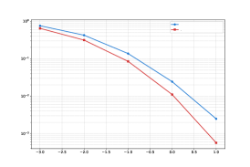
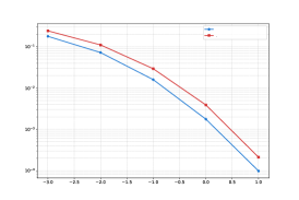
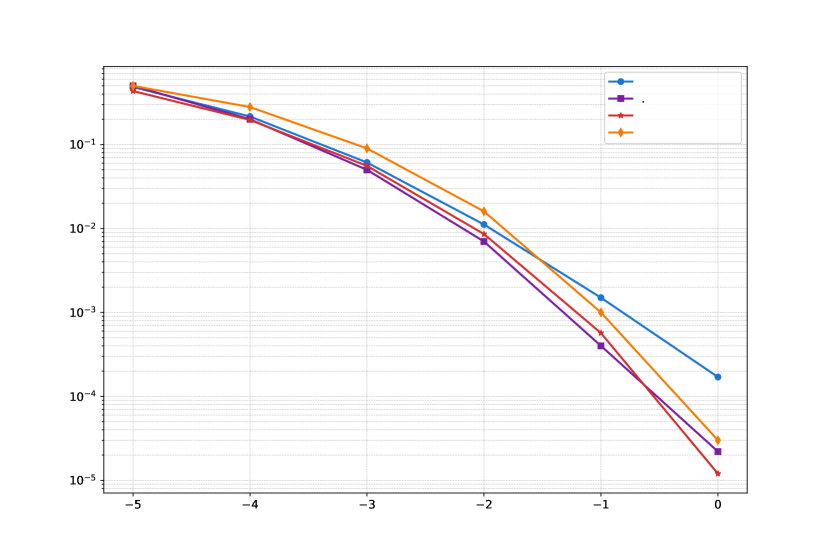
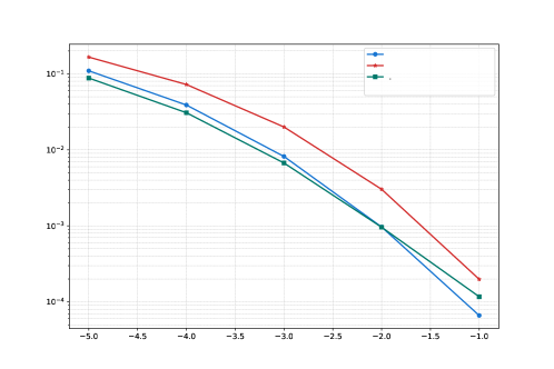
The core innovation of DeepPolar lies in its utilization of larger-size kernels, which enables the neural network to explore an expansive function space. This is complemented by a matching SC-like neural decoder, which is jointly trained on samples drawn from an AWGN channel. Larger kernel sizes are pivotal for DeepPolar achieving substantial performance improvements on the canonical AWGN channel, as evidenced in Fig. 1 for the case of . Through extensive empirical studies, we find that a kernel size is most effective in balancing bias and variance, enabling it to achieve significantly lower bit error rates over the baseline Polar and RM codes, as well as the KO(8,2) code, SOTA at this block length and rate. Additionally, we design a training curriculum that builds upon the inherent nested hierarchy of polar coding structures to accelerate training. This combination of principled coding-theoretic structures with a targeted training methodology is designed to enable effective generalization across the vast space of messages. In summary, we make the following contributions:
-
•
We propose DeepPolar, a novel generalization of Polar codes via large non-linear NN-based kernels.
-
•
DeepPolar outperforms the classical Polar and Reed-Muller codes, state-of-the-art binary linear codes, as well as KO codes, state-of-the-art ML-based codes, whilst scaling to various code rates.
-
•
We develop a principled curriculum-based training methodology that allows DeepPolar to generalize to the challenging high SNR regime.
2 Problem formulation and Background
2.1 Channel coding
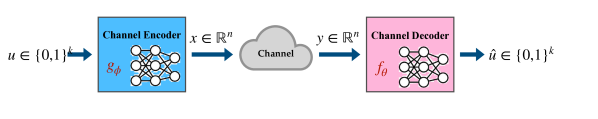
Channel coding is a technique to add redundancy to the transmission to make it robust against noise added by the communication channel. More precisely, let denote a block of information/message bits that we wish to transmit. A code consists of an encoder and decoder pair. The encoder maps these message bits into a binary codeword of length , i.e. . The codewords are mapped to real/complex values by modulation (eg, Binary Phase Shift Keying (BPSK)). The channel, denoted as , corrupts the codeword to its noisy version . Upon receiving the corrupted codeword, the decoder estimates the message bits as . The performance of the code is measured using standard error metrics such as Bit-Error-Rate (BER) or Block-Error-Rate (BLER): , whereas .
2.2 Polar codes
Polar codes, introduced by Erdal Arıkan (Arikan, 2009), are the first deterministic code construction to achieve the Shannon capacity while maintaining low encoding and decoding complexity. This section formally defines Polar codes and motivates our method.
Polar Encoding. A Polar code can be described by Polar(,,). Here, is the block length; for some integer , is the number of information bits, and represents the set of “frozen" bit positions. Typically, the positions corresponding to the noisiest bit channels arising due to polarization are chosen to be frozen. A polar encoder maps information bits to a binary codeword . The basic building block of Polar codes is the Plotkin transform: . This mapping for a pair of input bits can be represented by the matrix , transforming into , where denotes the XOR operation. Consistent with the coding theory literature, we term such a building block a kernel. The encoding matrix for block length is obtained by taking the Kronecker product of the base kernel times.
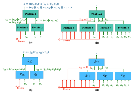
Utilizing this structure, the encoding can be efficiently performed via a recursive coordinate-wise application of the Plotkin transform on a binary tree, called the Plotkin tree. To encode a block of message bits , we first embed them into a source message vector , where and for some . Since the message block contains the information bits only at the indices pertaining to , the set is called the information set, and its complement the frozen set. We describe the encoding on a Plotkin tree via a small example, Polar(4,3) - illustrated in Fig. 3(a). Here, ={0}. Consider an input of size , . At the input level (depth 1), we freeze , i.e., and assign to the remaining positions. Applying the Plotkin transform, and . At the second level, we apply the same operation coordinatewise to these vectors i.e, and . The final encoded vector is the concatenation of the outputs from the second-level nodes i.e, . For a general polar code, the encoding proceeds similarly up to levels.
Polar decoding. The encoded messages are corrupted by a noisy channel . The successive cancellation (SC) algorithm is one of the most efficient decoders for Polar codes and is optimal asymptotically. The basic principle behind the SC algorithm is to sequentially decode each message bit according to the conditional likelihood given the corrupted codeword and previously decoded bits . LLR for bit can be computed as
| (1) |
SC decoding is described in detail in App. A.
Large kernel Polar codes. Polar codes are optimal (capacity-achieving) at asymptotic blocklengths due to the phenomenon of channel polarization. (Korada et al., 2010) prove that replacing the conventional kernel with an binary kernel () still results in polarization, provided this matrix is non-singular and not upper triangular under any column permutation. Further, large kernel polar codes that achieve capacity at shorter block lengths compared to conventional polar codes have been found, as indicated by better scaling exponents (Fazeli & Vardy, 2014; Fazeli et al., 2020). Notably, the kernel size must be expanded to 8 to surpass Arikan’s kernel, as no size 4 linear kernel offers an improved scaling exponent. While this generally translates to better finite-length performance, the complexity of decoding grows exponentially with kernel size (Trofimiuk & Trifonov, 2021); and decoders with comparable computational complexity (eg, SC decoding) are highly sub-optimal at short-to-medium block lengths (App. B).
Large kernel polar encoding and decoding proceeds similarly to conventional Polar codes via an kernel. An exemplar kernel with is simply the Kronecker product of with itself, . This is a Plotkin transform with 4 inputs, referred to as Plotkin-4. We illustrate this via an example of a code with kernel size in Fig. 3 . In this example, the message is input at the information positions . The remaining positions are frozen to 0. The kernel is applied in parallel to groups of bits. Mirroring the conventional polar encoding, we iteratively follow this process at each level of the tree. At the second level, we apply Plotkin-4 coordinatewise to the vectors to obtain the codeword .
In this work, we design a non-linear generalization of the polar coding and decoding structure by both expanding the kernel size and parameterizing them as neural networks. By expanding the design space to include non-linearity and larger kernels, we aim to discover more reliable codes within the Plotkin code family.
3 DeepPolar codes
3.1 Proposed Architecture
We design DeepPolar codes by generalizing the encoding and decoding structures of large kernel Polar codes. A DeepPolar code maps bits to a codeword , using the neural Plotkin tree of kernel size .
DeepPolar encoder. Building on the foundational encoding structure of Polar codes (Fig. 3a), which employs the recursive application of a binary kernel over a Plotkin tree, we introduce DeepPolar codes as a non-linear extension of this concept. The first major modification in our approach is expanding the conventional kernel to a larger kernel. While this generalization does not inherently lead to superior Polar codes at short blocklengths compared to the standard Arikan kernel, as discussed in the previous section (Fig. 3b), it lays the groundwork for further innovations in our design.
On the other hand, we generalize the Plotkin transform by replacing each XOR operation with a 2-input NN , where is the depth in the encoding tree, and is the index of the NN at depth . A DeepPolar inherits the same parameters as a Polar code. The encoding structure is analogous to conventional polar codes and is illustrated in Fig. 3(c) - DeepPolar (4,3) with . We use the same frozen set =0 as the conventional polar code. Applying the neural Plotkin transform, and . At the second level, we apply the kernel coordinatewise to these vectors. This coordinatewise operation is the key inductive bias in DeepPolar encoding. The final encoded vector is the concatenation of the outputs from the second-level nodes i.e, . For a general DeepPolar code, the encoding proceeds in a similar way upto levels.
Our work synergizes these two directions by employing a non-linear kernel of size . Fig. 3(d) illustrates DeepPolar , which mirrors the Plotkin-4 encoder for Polar. The encoding proceeds similarly, with neural networks replacing the Plotkin mapping. A power constraint, is enforced at the output of the encoder. App. E.5 discusses the DeepPolar encoder architecture in detail.
While large kernels in the context of Polar codes fail to improve over the standard 2x2 kernel, a critical distinguishing factor of DeepPolar is that we parameterize the kernel at each internal node of the Plotkin tree by a neural network . We hypothesize that this innovation unlocks performance gains through the expanded function space afforded by both non-linearization and the increased kernel size. Additionally, this formulation allows us to scale neural Polar codes to larger blocklengths and rates.
DeepPolar-SC decoder. To decode the received codewords corrupted by noise, we design the DeepPolar-SC decoder, a neural generalization of SC decoding. The DeepPolar-SC decoder consists of a decoding tree, consisting of decoding networks , matching every kernel . Notably, each decoding NN is applied coordinatewise and takes as input the LLR from the previous outputs, along with the inputs to the kernel. DeepPolar-SC is detailed in App. C.1.
3.2 Training methodology : Curriculum learning.
The primary challenge in training neural channel codes is the astronomical space of potential codewords; the task is to find a noise-robust mapping for each binary string in the -dimensional Boolean hypercube to a codeword in . This challenge is pronounced even in the short-to-medium blocklength regime we focus on, for instance, training a (256,37) code involves designing codewords in a 256-dimensional space. During training, we encounter a tiny fraction of the message space , making the NN’s ability to effectively generalize to unseen messages a pivotal factor in learning effective codes. While principled architectural choices are vital for generalization, the training methodology is equally important. Typically, an end-to-end training strategy would involve minimizing the binary cross entropy loss between the actual message bits and estimated message bits :
| (2) |
However, as highlighted in Sec. 4.4, direct training often does not generalize well to high SNR scenarios, characterized by infrequent error events.
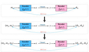
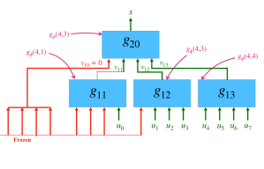
Curriculum. We address this by introducing a principled two-stage curriculum training procedure that capitalizes on the inherent nested hierarchy of Polar codes. We leverage two key properties of the Polar coding structure: (1)Hierarchy in k: A Polar subsumes all codewords of a code subsumes all the codewords of lower-rate subcodes . Curriculum training leveraging the hierarchy in improved both convergence speed and reliability in the context of neural polar decoding (Hebbar et al., 2023). In the first stage, we use a similar C2N curriculum to pretrain the parameters for each kernel. We progressively train encoder-decoder pairs for DeepPolar ( codes, for as highlighted in Fig. 4a), denoted by . (2)Hierarchy in n: In the Plotkin tree, an kernel is applied coordinatewise at each level of the Plotkin tree. In the second stage of our curriculum, we initialize each kernel in DeepPolar (,) encoder and decoder with the pre-trained kernels from the first stage, applied at all depths, as illustrated in Fig. 4b. For instance, and , which have three non-frozen inputs, are initialized by a pre-trained kernel . Such a systematic and phased training approach significantly enhances the network’s learning efficiency and generalizability (Sec. 4.4).
4 Main Results
4.1 Data generation.
We generate synthetic input data for the encoder by randomly sampling from a boolean hypercube i.e, . A randomly sampled white Gaussian noise is added to the output of the encoder. During training, the variance of the Gaussian noise is carefully chosen based on the length and rate of the desired channel code.
4.2 Results
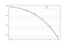
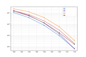
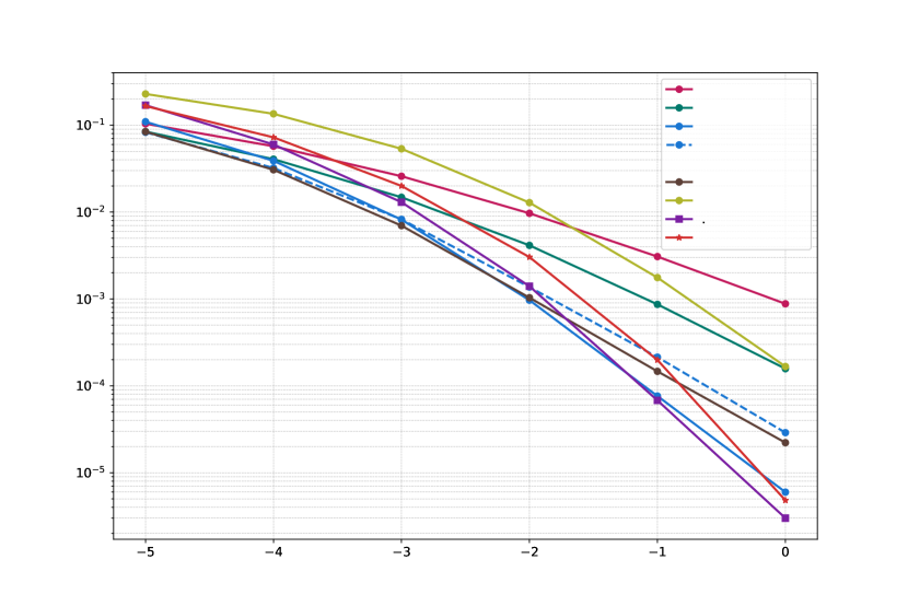
DeepPolar codes outperform Polar codes. As highlighted in Fig. 5, DeepPolar codes achieve enhanced performance over traditional Polar codes with SC decoding and Reed-Muller codes with Dumer decoding across a broad range of SNRs in the presence of additive white Gaussian noise (AWGN), in terms of bit error rate (BER). Notably, DeepPolar (256,37,) outperforms KO(8,2) (Fig. 5a), the state-of-the-art neural code mapping information bits to a length- codeword (Makkuva et al., 2021) in the short-to-medium blocklength regime. DeepPolar codes, owing to their Polar-like encoding framework, accommodate a much wider range of rates than KO codes that rely on the algebraic structure of RM codes. This versatility is illustrated in Fig. 5b and Fig. 5c, where DeepPolar codes outperform Polar codes across diverse rates and SNRs (cf. KO codes and RM codes do not exist for these rates). Further, DeepPolar is robust to non-AWGN deviations, achieving gains over Polar codes on fading channels and radar noise (App. D)
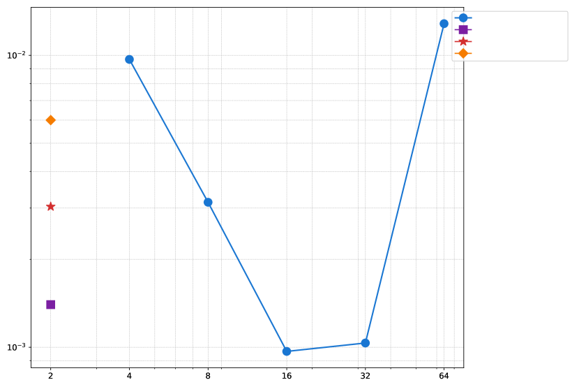
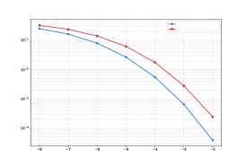
Effect of kernel size. Fig. 6 highlights that scaling the kernel size is crucial for effective training and DeepPolar outperforming baselines. An increase in kernel size expands the function space the encoder can represent, facilitating learning more robust representations. However, empirical experiments reveal that using , which results in an encoding and decoding tree of depth 2, is a good heuristic. Indeed, Fig. 1 highlights significant improvements in performance upto , whereas further scaling leads to a decline. This trend indicates a bias-variance tradeoff, suggesting the ideal kernel size strikes a balance between model complexity and its generalization capabilities.
4.3 Interpretation
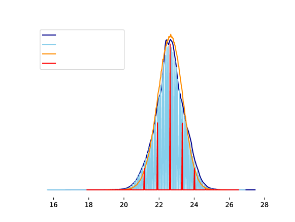
Interpreting the encoder. To interpret the encoder, we examine the distribution of pairwise distances between codewords (Fig. 7). Gaussian codebooks achieve capacity and are optimal asymptotically (Shannon, 1948). Remarkably, the distribution of DeepPolar codewords closely resembles that of the Gaussian codebook. This surprising phenomenon has also been observed in the closely related KO codes and is a testament to the potential of the marriage between efficient algebraic code structures and DL.
Interpreting the decoder. In our study, the training loss used is binary cross entropy (BCE), which serves as a surrogate for the bit error rate (BER). However, it is important to recognize that optimizing for BER does not necessarily translate to improved block error rate (BLER), an important figure of merit in practical systems. Our observations, as indicated in Fig. 8a, show that DeepPolar underperforms in BLER compared to baseline methods (See App. F for more results). The BLER, defined as , can be expressed as the cumulative probability of bit errors occurring at each position when no errors were made in the previous ones:
| (3) |
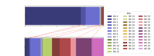
An analysis of error distribution (Fig. 8b) reveals notable differences between SC and DeepPolar-SC decoders despite both employing a sequential decoding approach. Due to the effect of channel polarization, most errors in the polar decoding tend to occur at bit position 0, which predominantly drives the BLER. In contrast, errors in DeepPolar decoding are more evenly distributed across various bit positions. This uniformity is a consequence of the BCE loss prioritizing BER over BLER. This trade-off leads to a marginal decrease in BLER performance. Identifying a stable loss function directly targeting BLER, is an interesting direction for future research.
4.4 Ablation studies
DeepPolar-Binary Compared to canonical coding schemes, a real-valued coding scheme like DeepPolar offers distinct advantages by integrating modulation and coding schemes. However, practical systems may have hard symbol-level power constraints, necessitating code bits to be integers . Hence, it is beneficial to have the ability to learn a binary code while maintaining the structure of DeepPolar.
To achieve this, a trained DeepPolar model is fine-tuned with a Straight Through Estimator (STE) (Hubara et al., 2016) and a binarization module, resulting in a binary version, DeepPolar-binary, akin to the methodology in (Jiang et al., 2019b). Fig. 5a highlights that there is a loss incurred with respect to DeepPolar. This underscores the contribution of joint coding and modulation to DeepPolar’s performance. Nevertheless, DeepPolar-binary not only surpasses the performance of the traditional Polar code but also closely matches that of KO codes. Additionally, the distance profile of DeepPolar-binary (Fig. 7) indicates it preserves Gaussian codebook-like distance properties, reinforcing the potential of non-linear binary codes derived from polarization-inducing structures. This exploration opens avenues for future research, particularly in interpreting these codes to develop novel, efficient encoders and decoders leveraging non-linear polarization-based methods.
Effect of curriculum. Ensuring reliable performance of neural codes at high SNR levels is a significant challenge, primarily due to the sparse occurrence of error events in this regime. This challenge often leads to a phenomenon known as an error floor, where the error rate improvement of a code stagnates beyond a certain SNR (Jamali et al., 2021b). This issue is not exclusive to neural codes, as it’s also encountered in classical codes like LDPC and Turbo codes. While training hyperparameters such as SNR scheduling and batch sizes affect high SNR performance - the structure of the code also plays a part. Notably, algebraic codes like polar codes do not suffer from error floors. Driven by this intuition, our curriculum design (Sec. 3.2) reinforces the Plotkin code structure, leading to better generalization. This strategy has been effective, as highlighted in Fig. 6, where implementing a curriculum markedly enhances code performance at higher SNRs.
4.5 Computational Complexity
In our study, we introduce a novel non-linear generalization of the Polar code’s encoding and decoding structures and achieve substantial improvements in reliability. Another essential aspect of evaluating an algorithm is the computational complexity, which has a direct impact on power consumption. Polar codes are favored due to their relatively low-complexity encoding and decoding algorithms. However, in practice, CRC-aided list decoders are used, which substantially increases the decoding complexity. DeepPolar is a non-linear generalization of Polar codes via neural-network-based kernels on the Plotkin tree. The DeepPolar SC-decoder is a kernel-wise sequential decoder inspired by the SC algorithm. For the case of DeepPolar , the encoder and decoder have 0.1M and 1.6M parameters, respectively, which we did not optimize in this project. Our findings serve as constructive proof that non-linear polar codes with large kernels can outperform the state-of-the-art. Further, we demonstrate the viability of effective binary codes with a large-kernel Polar structure, complete with efficient decoders. This opens avenues for further examination of these codebooks to inform the development of low-complexity solutions. Notably, the complexity of neural codes can be reduced significantly without performance degradation by complexity-aware architecture design (eg, TinyKO (Makkuva et al., 2021)). Our preliminary experiments with DeepPolar-parallel (App. C.2), which reduces the decoder parameter count by 8x, have already demonstrated improved performance at lower complexity. Further, several techniques are used in practice, like distillation, quantization, and pruning, among others, to reduce the computational overhead of a neural algorithm. This is important and interesting future work beyond the scope of this paper.
5 Related work
The application of machine learning to channel coding has been an active area of research in recent years. The majority of existing works focus on decoding existing codes, aiming to achieve better reliability and robustness, and in some cases, lower decoding complexity (Kim et al., 2018b; Nachmani et al., 2016; Dörner et al., 2017; Vasić et al., 2018; Nachmani & Wolf, 2019; Jiang et al., 2019a; Chen & Ye, 2021; Jamali et al., 2021a; Choukroun & Wolf, 2022a, b; Hebbar et al., 2022; Aharoni et al., 2023). In the context of polar codes, several neural decoders have been proposed (Cammerer et al., 2017b, a; Doan et al., 2018; Hebbar et al., 2023). In another line of work, (Ebada et al., 2019; Liao et al., 2021; Li et al., 2021; Miloslavskaya et al., 2023; Ankireddy et al., 2024) use deep learning to identify optimal polar code frozen positions without altering the design of encoder and decoder.
In contrast, jointly learning both encoders and decoders is a more challenging problem, and very few works in the literature exist. A common theme is the incorporation of principled coding-theoretic encoding and decoding structures. TurboAE (Jiang et al., 2019b), and follow-up works (Jiang et al., 2020b, a; Chahine et al., 2021; Saber et al., 2022; Chahine et al., 2022a; Wang et al., 2023), use sequential encoding and decoding along with interleaving of input bits, inspired by Turbo codes (Berrou et al., 1993). KO codes (Makkuva et al., 2021) generalize Reed-Muller encoding and Dumer decoding by replacing selected components in the Plotkin tree with neural networks. ProductAE (Jamali et al., 2021b) generalizes two-dimensional product codes to scale neural codes to larger block lengths. In a similar vein, our work generalizes the coding structures of large-kernel Polar codes by using non-linear kernels parameterized by NNs.
Deep learning-based schemes for channels with feedback is another active area of research (Kim et al., 2018a; Safavi et al., 2021; Chahine et al., 2022b; Ozfatura et al., 2022, 2023b, 2023a; Kim et al., 2023). Furthermore, breaking the conventional wisdom that neural codes are hard to interpret, (Devroye et al., 2022) derives a closed-form approximation of binarized TurboAE codes via mixed integer linear programming and other techniques. The task of analytically approximating and understanding binarized DeepPolar codes remains a promising subject for future research.
6 Conclusion
In this work, we introduce DeepPolar codes, a new class of non-linear generalizations of large-kernel Polar codes. DeepPolar codes generalize to various rates and blocklengths, and outperform the current state-of-the-art in BER.
Impact Statement. This paper presents work whose goal is to advance the field of channel coding using machine learning. There are many potential societal consequences of our work, none of which we feel must be specifically highlighted here.
References
- 3GPP (2018) 3GPP. Multiplexing and channel coding. Technical Specification 38.212, 3rd Generation Partnership Project (3GPP), 2018. Release 15.
- Abbasi & Viterbo (2020) Abbasi, F. and Viterbo, E. Large kernel polar codes with efficient window decoding. IEEE Transactions On Vehicular Technology, 69(11):14031–14036, 2020.
- Aharoni et al. (2023) Aharoni, Z., Huleihel, B., Pfister, H. D., and Permuter, H. H. Data-driven polar codes for unknown channels with and without memory. In 2023 IEEE International Symposium on Information Theory (ISIT), pp. 1890–1895. IEEE, 2023.
- Ankireddy et al. (2024) Ankireddy, S. K., Hebbar, S. A., Wan, H., Cho, J., and Zhang, C. Nested construction of polar codes via transformers. arXiv preprint arXiv:2401.17188, 2024.
- Arikan (2009) Arikan, E. Channel polarization: A method for constructing capacity-achieving codes for symmetric binary-input memoryless channels. IEEE Transactions on information Theory, 55(7):3051–3073, 2009.
- Arıkan (2019) Arıkan, E. From sequential decoding to channel polarization and back again. arXiv preprint arXiv:1908.09594, 2019.
- Berrou et al. (1993) Berrou, C., Glavieux, A., and Thitimajshima, P. Near shannon limit error-correcting coding and decoding: Turbo-codes. 1. In Proceedings of ICC’93-IEEE International Conference on Communications, volume 2, pp. 1064–1070. IEEE, 1993.
- Bioglio et al. (2020) Bioglio, V., Condo, C., and Land, I. Design of polar codes in 5g new radio. IEEE Communications Surveys & Tutorials, 23(1):29–40, 2020.
- Cammerer et al. (2017a) Cammerer, S., Gruber, T., Hoydis, J., and Ten Brink, S. Scaling deep learning-based decoding of polar codes via partitioning. In GLOBECOM 2017-2017 IEEE global communications conference, pp. 1–6. IEEE, 2017a.
- Cammerer et al. (2017b) Cammerer, S., Leible, B., Stahl, M., Hoydis, J., and ten Brink, S. Combining belief propagation and successive cancellation list decoding of polar codes on a gpu platform. In 2017 IEEE international conference on acoustics, speech and signal processing (ICASSP), pp. 3664–3668. IEEE, 2017b.
- Chahine et al. (2021) Chahine, K., Ye, N., and Kim, H. Deepic: Coding for interference channels via deep learning. arXiv preprint arXiv:2108.06028, 2021.
- Chahine et al. (2022a) Chahine, K., Jiang, Y., Nuti, P., Kim, H., and Cho, J. Turbo autoencoder with a trainable interleaver. In ICC 2022-IEEE International Conference on Communications, pp. 3886–3891. IEEE, 2022a.
- Chahine et al. (2022b) Chahine, K., Mishra, R., and Kim, H. Inventing codes for channels with active feedback via deep learning. IEEE Journal on Selected Areas in Information Theory, 3(3):574–586, 2022b.
- Chen & Ye (2021) Chen, X. and Ye, M. Cyclically equivariant neural decoders for cyclic codes. arXiv preprint arXiv:2105.05540, 2021.
- Choukroun & Wolf (2022a) Choukroun, Y. and Wolf, L. Denoising diffusion error correction codes. arXiv preprint arXiv:2209.13533, 2022a.
- Choukroun & Wolf (2022b) Choukroun, Y. and Wolf, L. Error correction code transformer. arXiv preprint arXiv:2203.14966, 2022b.
- Devroye et al. (2022) Devroye, N., Mohammadi, N., Mulgund, A., Naik, H., Shekhar, R., Turán, G., Wei, Y., and Žefran, M. Interpreting deep-learned error-correcting codes. In 2022 IEEE International Symposium on Information Theory (ISIT), pp. 2457–2462, 2022. doi: 10.1109/ISIT50566.2022.9834599.
- Doan et al. (2018) Doan, N., Hashemi, S. A., and Gross, W. J. Neural successive cancellation decoding of polar codes. In 2018 IEEE 19th international workshop on signal processing advances in wireless communications (SPAWC), pp. 1–5. IEEE, 2018.
- Dörner et al. (2017) Dörner, S., Cammerer, S., Hoydis, J., and Ten Brink, S. Deep learning based communication over the air. IEEE Journal of Selected Topics in Signal Processing, 12(1):132–143, 2017.
- Ebada et al. (2019) Ebada, M., Cammerer, S., Elkelesh, A., and ten Brink, S. Deep learning-based polar code design. In 2019 57th Annual Allerton Conference on Communication, Control, and Computing (Allerton), pp. 177–183. IEEE, 2019.
- Fazeli & Vardy (2014) Fazeli, A. and Vardy, A. On the scaling exponent of binary polarization kernels. In 2014 52nd Annual Allerton Conference on Communication, Control, and Computing (Allerton), pp. 797–804. IEEE, 2014.
- Fazeli et al. (2020) Fazeli, A., Hassani, H., Mondelli, M., and Vardy, A. Binary linear codes with optimal scaling: Polar codes with large kernels. IEEE Transactions on Information Theory, 67(9):5693–5710, 2020.
- Gupta et al. (2021) Gupta, B., Yao, H., Fazeli, A., and Vardy, A. Polar list decoding for large polarization kernels. In 2021 IEEE Globecom Workshops (GC Wkshps), pp. 1–6. IEEE, 2021.
- Hebbar et al. (2022) Hebbar, S. A., Mishra, R. K., Ankireddy, S. K., Makkuva, A. V., Kim, H., and Viswanath, P. Tinyturbo: Efficient turbo decoders on edge. In 2022 IEEE International Symposium on Information Theory (ISIT), pp. 2797–2802. IEEE, 2022.
- Hebbar et al. (2023) Hebbar, S. A., Nadkarni, V. V., Makkuva, A. V., Bhat, S., Oh, S., and Viswanath, P. Crisp: Curriculum based sequential neural decoders for polar code family. In International Conference on Machine Learning, pp. 12823–12845. PMLR, 2023.
- Hubara et al. (2016) Hubara, I., Courbariaux, M., Soudry, D., El-Yaniv, R., and Bengio, Y. Binarized neural networks. Advances in neural information processing systems, 29, 2016.
- Jamali et al. (2021a) Jamali, M. V., Liu, X., Makkuva, A. V., Mahdavifar, H., Oh, S., and Viswanath, P. Reed-muller subcodes: Machine learning-aided design of efficient soft recursive decoding. In 2021 IEEE International Symposium on Information Theory (ISIT), pp. 1088–1093. IEEE, 2021a.
- Jamali et al. (2021b) Jamali, M. V., Saber, H., Hatami, H., and Bae, J. H. Productae: Towards training larger channel codes based on neural product codes. arXiv preprint arXiv:2110.04466, 2021b.
- Jiang et al. (2019a) Jiang, Y., Kannan, S., Kim, H., Oh, S., Asnani, H., and Viswanath, P. Deepturbo: Deep turbo decoder. In 2019 IEEE 20th International Workshop on Signal Processing Advances in Wireless Communications (SPAWC), pp. 1–5. IEEE, 2019a.
- Jiang et al. (2019b) Jiang, Y., Kim, H., Asnani, H., Kannan, S., Oh, S., and Viswanath, P. Turbo autoencoder: Deep learning based channel codes for point-to-point communication channels. In Advances in Neural Information Processing Systems, pp. 2758–2768, 2019b.
- Jiang et al. (2020a) Jiang, Y., Kim, H., Asnani, H., Kannan, S., Oh, S., and Viswanath, P. Joint channel coding and modulation via deep learning. In 2020 IEEE 21st International Workshop on Signal Processing Advances in Wireless Communications (SPAWC), pp. 1–5. IEEE, 2020a.
- Jiang et al. (2020b) Jiang, Y., Kim, H., Asnani, H., Oh, S., Kannan, S., and Viswanath, P. Feedback turbo autoencoder. In ICASSP 2020-2020 IEEE International Conference on Acoustics, Speech and Signal Processing (ICASSP), pp. 8559–8563. IEEE, 2020b.
- Kim et al. (2018a) Kim, H., Jiang, Y., Kannan, S., Oh, S., and Viswanath, P. Deepcode: Feedback codes via deep learning. Advances in neural information processing systems, 31, 2018a.
- Kim et al. (2018b) Kim, H., Jiang, Y., Rana, R., Kannan, S., Oh, S., and Viswanath, P. Communication algorithms via deep learning. arXiv preprint arXiv:1805.09317, 2018b.
- Kim et al. (2023) Kim, J., Kim, T., Love, D., and Brinton, C. Robust non-linear feedback coding via power-constrained deep learning. arXiv preprint arXiv:2304.13178, 2023.
- Korada et al. (2010) Korada, S. B., Şaşoğlu, E., and Urbanke, R. Polar codes: Characterization of exponent, bounds, and constructions. IEEE Transactions on Information Theory, 56(12):6253–6264, 2010.
- Li et al. (2021) Li, Y., Chen, Z., Liu, G., Wu, Y.-C., and Wong, K.-K. Learning to construct nested polar codes: An attention-based set-to-element model. IEEE Communications Letters, 25(12):3898–3902, 2021.
- Liao et al. (2021) Liao, Y., Hashemi, S. A., Cioffi, J. M., and Goldsmith, A. Construction of polar codes with reinforcement learning. IEEE Transactions on Communications, 70(1):185–198, 2021.
- Makkuva et al. (2021) Makkuva, A. V., Liu, X., Jamali, M. V., Mahdavifar, H., Oh, S., and Viswanath, P. Ko codes: inventing nonlinear encoding and decoding for reliable wireless communication via deep-learning. In International Conference on Machine Learning, pp. 7368–7378. PMLR, 2021.
- Miloslavskaya et al. (2023) Miloslavskaya, V., Li, Y., and Vucetic, B. Design of compactly specified polar codes with dynamic frozen bits based on reinforcement learning. IEEE Transactions on Communications, 2023.
- Nachmani & Wolf (2019) Nachmani, E. and Wolf, L. Hyper-graph-network decoders for block codes. Advances in Neural Information Processing Systems, 32:2329–2339, 2019.
- Nachmani et al. (2016) Nachmani, E., Be’ery, Y., and Burshtein, D. Learning to decode linear codes using deep learning. In 2016 54th Annual Allerton Conference on Communication, Control, and Computing (Allerton), pp. 341–346. IEEE, 2016.
- Niu & Chen (2012) Niu, K. and Chen, K. Crc-aided decoding of polar codes. IEEE communications letters, 16(10):1668–1671, 2012.
- Ozfatura et al. (2022) Ozfatura, E., Shao, Y., Perotti, A. G., Popović, B. M., and Gündüz, D. All you need is feedback: Communication with block attention feedback codes. IEEE Journal on Selected Areas in Information Theory, 3(3):587–602, 2022.
- Ozfatura et al. (2023a) Ozfatura, E., Bian, C., and Gündüz, D. Do not interfere but cooperate: A fully learnable code design for multi-access channels with feedback. In 2023 12th International Symposium on Topics in Coding (ISTC), pp. 1–5. IEEE, 2023a.
- Ozfatura et al. (2023b) Ozfatura, E., Shao, Y., Ghazanfari, A., Perotti, A., Popovic, B., and Gündüz, D. Feedback is good, active feedback is better: Block attention active feedback codes. In ICC 2023-IEEE International Conference on Communications, pp. 6652–6657. IEEE, 2023b.
- Saber et al. (2022) Saber, H., Hatami, H., and Bae, J. H. List autoencoder: Towards deep learning based reliable transmission over noisy channels. In GLOBECOM 2022-2022 IEEE Global Communications Conference, pp. 1454–1459. IEEE, 2022.
- Safavi et al. (2021) Safavi, A. R., Perotti, A. G., Popovic, B. M., Mashhadi, M. B., and Gunduz, D. Deep extended feedback codes. arXiv preprint arXiv:2105.01365, 2021.
- Shannon (1948) Shannon, C. E. A mathematical theory of communication. The Bell system technical journal, 27(3):379–423, 1948.
- Trofimiuk & Trifonov (2021) Trofimiuk, G. and Trifonov, P. Window processing of binary polarization kernels. IEEE Transactions on Communications, 69(7):4294–4305, 2021.
- Vasić et al. (2018) Vasić, B., Xiao, X., and Lin, S. Learning to decode ldpc codes with finite-alphabet message passing. In 2018 Information Theory and Applications Workshop (ITA), pp. 1–9. IEEE, 2018.
- Wang et al. (2023) Wang, L., Saber, H., Hatami, H., Jamali, M. V., and Bae, J. H. Rate-matched turbo autoencoder: A deep learning based multi-rate channel autoencoder. In ICC 2023-IEEE International Conference on Communications, pp. 6355–6360. IEEE, 2023.
Appendix A Successive Cancellation decoder
Here we look at the Successive Cancellation Decoding algorithm, provided in (Arikan, 2009). As the name suggests, the SC decoding algorithm decodes the bits sequentially, starting with . A frozen bit node is always decoded as . And while decoding the , the available bits to which are represented by the vector are used according to decode according to the following rule:
| (4) |
where is the set of information positions.
The probability calculations are computationally easier and less prone to round-off errors in the log domain. Hence, we consider LLRs instead of probabilities to avoid numerical overflows. LLR for bit is defined as:
Hence, the decision rule changes as follows:
| (5) |
The binary tree structure of a polar code can be exploited to simplify the successive cancellation decoding. The binary tree has stages with numbering from . Each stage contains nodes with each node corresponding to bits.
In order, traversal of the tree is done to perform the successive cancellation decoding. At each node, messages are passed as shown:
Each node passes LLR corresponding LLR values, namely , to the child nodes and sends the estimated hard bits at the sage, namely , o the parent node. The left and right messages, and are calculated as:
| (6) |
| (7) |
We define two functions to perform these operations, namely and , defined as:
| (8) |
But the function is computationally expensive, and hence, we approximate it to a hardware-friendly version using min-sum approximation as follows:
| (9) |
where sign gives the sign of input and min gives the minimum of the two inputs.
The algorithm starts from the root node of the tree, which is level , and traverses to the leaf node, which is level . For each node, the following set of operations occurs.
-
1.
If the current node has a left child that was not visited, calculate and move to the left child.
-
2.
If the current node has a right child that was not visited, calculate and move to the right child.
-
3.
If both the messages from child nodes are available, calculate and move to the parent node.
Once the leaf node is reached, decisions are made based on the sign of the corresponding LLR using the binary quantizer function as:
| (10) |
where is defined as:
Appendix B Large kernel Polar codes
One of the drawbacks of larger kernel Polar codes in practice is the lack of efficient low-complexity decoding algorithms. The SC decoding operation for larger kernel Polar codes () is similar to the original polar codes. While the operations remain the same, iteratively computing the probabilities increases exponentially with respect to as , making it prohibitively expensive for very large kernels (Abbasi & Viterbo, 2020; Gupta et al., 2021). Iteratively, the relation can be expressed as
which is the probability for path given channel output .
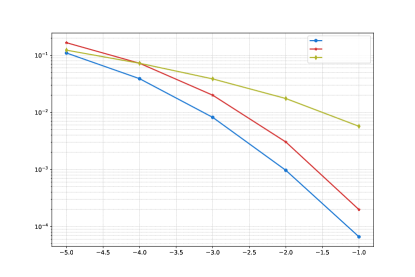
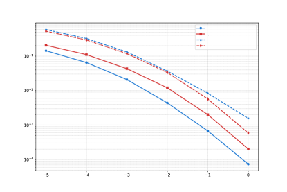
To demonstrate the ineffectiveness of current SC decoding strategies for larger kernel Polar codes at short-to-medium blocklengths, we consider a kernel size of (Trofimiuk & Trifonov, 2021) with SC list decoding and compare it with Polar code with SC decoding for and DeepPolar code of . We see from Fig. 11 that for a code, a larger kernel Polar code is orders of magnitude worse than Polar code with . Notably, the DeepPolar code of is better than the Polar code of by more than dB, demonstrating the efficacy of DeepPolar codes for larger kernels.
Appendix C DeepPolar Decoders
C.1 DeepPolar-SC Decoder
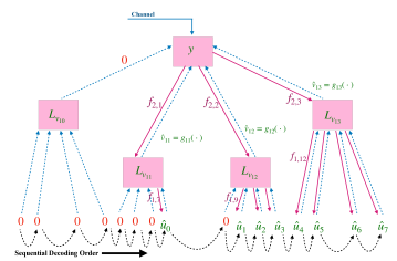
Decoding of DeepPolar for large kernels is depicted in Fig. 13 for DeepPolar (16,8,). The frozen positions are not decoded and are directly set to 0, including the full of the first kernel. Beginning with the first information position, is estimated based on the received values using sub-kernel . Now, the decoding of the two kernels is complete and sent to the parent node to begin the decoding of kernel 3. Using the received values and , sub-kernel estimates the next non-frozen position . Next, using and , sub-kernel decodes the next non-frozen position . This process is continued until kernel-3 is decoded completely, after which the decoding of kernel-4 starts in the same manner and continues until all bits are estimated.
To summarise, successive cancellation decoding of DeepPolar involves sequentially decoding one kernel of size at a time. Decoding the kernel is again performed in a successive fashion, where each bit is decoded by the corresponding component decoder or sub-kernel.
C.2 DeepPolar-parallel decoder
A major drawback of SC decoding and its variants like SCL decoders is the latency overhead due to sequential decoding. This drawback is inherently present in the DeepPolar-SC decoder. One method to break this latency barrier, whilst reducing the computational complexity of the decoder is to replace the SC-style NN decoders for a kernel at the lowest depth, by a single 3-layer FCNN, with hidden size 64, that decodes bits in one shot. We refer to this as DeepPolar-parallel. This resulted in an immediate reduction of 8x in parameter count compared to DeepPolar-SC while achieving better reliability, as highlighted in Fig. 14.
These preliminary results hint at the existence of low-complexity architectures that provide comparable performance at a much lower complexity. This is a promising direction of future exploration.
Appendix D Robustness to non-AWGN channels
Traditionally, the theoretical study of code design has been limited to AWGN channels. This is because of the difficulty in achieving a closed-form expression for the performance of the code in the presence of more complicated channel or noise conditions. But in practice, the channel experienced is far from AWGN, so testing any code on such varying channel conditions is crucial. We are specifically interested in the robustness of DeepPolar codes designs for AWGN channel, against non-AWGN channels .ie., we test and compare the performance without retaining.

First, we consider Rayleigh fast-fading channel with AWGN noise. Rayleigh fading is considered a suitable model for signal propagation in tropospheric and ionospheric environments, as well as for the effect of heavily built-up urban areas on radio signals. Mathematically, the channel model can be approximated as
where is the fading coefficient and is the Gaussian noise. Note that the fading coefficient changes for every symbol in the codeword, making it a much worse channel than the AWGN channel. As seen from Fig. 15a, the DeepPolar code demonstrates a gain of up to 0.3 dB compared to Polar(256,37), demonstrating the robustness of the learned code.
Next, we consider a bursty noise channel. Bursty noise, also known as popcorn noise, is a common type of noise encountered in semi-conductors. It can be described mathematically as
where is the Gaussian noise and with probability and with probability is the bursty noise. For our experiment, we choose and . As seen from Fig. 15b, the DeepPolar code demonstrates a gain of up to 0.25 dB compared to Polar(256,37) in the presence of bursty noise.
Appendix E Experimental details
The complete source code is provided at: https://anonymous.4open.science/r/deeppolar-ED52
E.1 Training algorithm
We follow a training strategy similar to KO codes (Makkuva et al., 2021), where the encoder and decoder networks are trained in an alternating optimization, described below.
E.2 Training SNR and number of steps
Choosing the right SNR is critical to avoid local optima during training. Choosing a very low SNR will result in the noise dominating the training data, and as a result, the training may not converge. On the contrary, choosing a very high SNR will not provide sufficient error events for the model to learn from. Through empirical testing, we find that a training SNR of 0 dB for the encoder and -2 dB for the decoder works best. Intuitively, this can be interpreted as learning a good decoder being much harder than learning a good encoder, as the decoder has to work with noisy data, whereas the encoder always takes clean input.
Continuing on this theme, we also observe that training the encoder for fewer iterations is sufficient compared to the decoder. In our experiments, we train the encoder 10x fewer steps than the decoder.
E.3 Large batch size and gradient accumulation
Having a large batch size during training is desirable for stable training. Larger batch sizes will capture the statistics of the underlying distribution more accurately, improving the accuracy of normalization using the mean and variance of the batch. Moreover, a larger batch size also reduces the noise in the gradients computed. In our experiments, we considered a batch size of up to 20000 and further used gradient accumulation techniques to simulate an even larger batch size.
E.4 Hyperparameter choices for DeepPolar (256,37)
The hyperparamters used for training DeepPolar (256,37,) are listed below.
| Hyperparameter | Value |
| Batch size () | 20,000 |
| Encoder training SNR | 0 dB |
| Decoder training SNR | -2 dB |
| Total epochs () | 2,000 |
| Encoder steps per epoch () | 20 |
| Decoder steps per epoch () | 200 |
| Encoder learning rate () | |
| Decoder learning rate () | |
| Optimizer | Adam |
E.5 Architecture for DeepPolar (256,37)
E.5.1 Encoder
The encoder is a collection of kernels of size , each of which is modeled by a neural network . The encoder kernel is responsible for encoding inputs. The architecture for is given as follows:
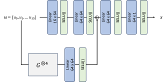
A crucial design choice is to make the polar-encoded features available to the encoding network via a skip connection. DeepPolar codes rely on the encoding and decoding structures of Polar codes, and the features corresponding to polar codes are indeed informative. Further, since it is harder for NNs to learn multiplicative policies, this side information proves to be useful in the learning process.
However, it is noteworthy that the learned DeepPolar codes, as well as DeepPolar-binary codes do not resemble polar codes, both in the mapping as well as the code distance spectrum.
E.5.2 Decoder
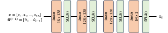
The encoder is a collection of kernels of size , each of which is modeled by a neural network . The decoder kernel contains sub-networks , each responsible for decoding the kernel’s position. The architecture for is given as follows:
Appendix F Additional results
F.1 Block Error Rate