Beyond unital noise in variational quantum algorithms: noise-induced barren plateaus and fixed points

Abstract

Variational quantum algorithms (VQAs) hold much promise but face the challenge of exponentially small gradients. Unmitigated, this barren plateau (BP) phenomenon leads to an exponential training overhead for VQAs. Perhaps the most pernicious are noise-induced barren plateaus (NIBPs), a type of unavoidable BP arising from open system effects, which have so far been shown to exist for unital noise channels. Here, we generalize the study of NIBPs to more general completely positive, trace-preserving maps, establishing the existence of NIBPs in the unital and single-qubit non-unital cases and tightening to logarithmic earlier bounds on the circuit depth at which an NIBP appears. We identify the associated phenomenon of noise-induced fixed points (NIFP) of the VQA cost function and prove its existence for both unital and single-qubit non-unital noise. Along the way, we extend the parameter shift rule of VQAs to the noisy setting. We provide rigorous bounds in terms of the relevant parameters that give rise to NIBPs and NIFPs, along with numerical simulations of the depolarizing and amplitude-damping channels that illustrate our analytical results.

I Introduction

Variational quantum algorithms (VQAs) are promising applications of quantum computing in the NISQ era [1, 2, 3, 4]. These algorithms leverage a customizable quantum circuit design, integrating both quantum and classical computation capabilities. Using parameterized quantum circuits, they compute problem-specific cost functions, followed by classical optimization to iteratively update the parameters. This hybrid quantum-classical optimization process continues until predefined termination criteria are met.

Previous studies have demonstrated that VQA circuits operable within the existing noise levels and hardware connectivity limitations of the NISQ era, already find applications across diverse domains, such as quantum optimization [5, 6, 7], quantum optimal control [8], linear systems [9, 10, 11], quantum metrology [12, 13], quantum compiling [14, 15], quantum error correction [16, 17], quantum machine learning [18, 19] and quantum simulation [20, 21, 22]. Moreover, VQA has been established as a universal model of quantum computation [23].

Despite their comparable computational power to other quantum models and demonstrated advantages, VQAs exhibit inherent constraints that present scalability challenges for problems of arbitrary scale. Specifically, VQAs for random circuits suffer from exponentially vanishing gradients, commonly referred to as the Barren Plateau (BP) phenomenon [24, 25, 26, 27, 28, 29, 30, 31, 32]. This phenomenon renders the parameter training step asymptotically impossible for circuits with a sufficiently large number of qubits $n$, even at shallow circuit depth.

Here, we study noise-induced barren plateaus (NIBPs), which emerge under decoherence-induced noise [33]. NIBPs were previously shown to be present in sufficiently deep circuits subjected to unital maps [31]. This holds true even in constant-width or non-random circuits. Alternatively, NIBPs exist under strictly contracting noise maps when the parameter shift rule (PSR) [18, 34] is applicable [35].

Unlike other BP types, for which mitigation strategies have been proposed [36, 25, 37, 38, 39, 40, 41, 42, 43, 44, 45], it remains unclear whether NIBPs can be similarly mitigated. Experimental investigations on small systems have suggested that error mitigation (EM) techniques enable VQAs to more closely approach the true ground-state energy [46]. Clifford Data Regression has proven effective in mitigating errors and reversing the concentration of cost function values [47]. Nevertheless, it is noteworthy that the majority of EM protocols do not enhance trainability or even exacerbate the lack of trainability. Additionally, post-processing expectation values of noisy circuits is not advantageous in the context of NIBP [48]. Previous work suggests that stochastic noise could be helpful for training VQAs [49]; an interesting open question that remains is whether there is an intermediate noise regime where we can train VQAs by exploiting noise.

In this work, we extend the study of NIBPs to completely positive trace-preserving (CPTP) maps, including both unital and single-qubit non-unital maps. We analytically derive the scaling of the cost function gradient as a function of circuit width $n$, circuit depth $L$, and noise strength. We find that the single-qubit non-unital noise need not necessarily give rise to NIBPs, but instead exhibits a different phenomenon, which we refer to as a noise-induced fixed point (NIFP). Moreover, we simplify the NIBP derivation compared to Ref. [31], guided by the intuition gained by considering the effect of noise on the single-qubit Bloch sphere. We generalize this to $n$-qubit systems via the coherence vector and compute derivatives of the cost function via the PSR. In addition, we investigate the applicability of the PSR under control noise and random unitary noise and assess the impact of these noise types on the bounds we derive. We find analytical expressions for the dependence of the circuit depth $L$ on relevant noise and circuit parameters that give rise to NIBP and NIFP. Our analytical results are supported by numerical simulations.

This paper is organized as follows. Background results regarding VQA, PSR, the coherence vector, and characteristics of CPTP noise maps are presented in Section II. Section III extends the PSR analysis to scenarios involving noise. We study the effects of single-qubit non-unital and general unital noise in Section IV and Section V, respectively. In the unital case, we reprove that NIBP is always present. In the single-qubit non-unital case, we find new results, in particular the phenomenon of NIFP. Our theoretical findings are supported by numerical simulations in Section VI. We summarize our findings in Section VII.

II Preliminaries

In this section, we review pertinent technical details and establish the notation we use to derive our results.

II.1 VQA and PSR

We adopt the variational quantum algorithm (VQA) framework of Ref. [31] and consider a general class of parameterized unitary ansatzes:

$$U(\boldsymbol{\theta}) =\Pi_{l=L}^{1}U_{l}(\boldsymbol{\theta}_{l}),$$ (1a)

$$U_{l}(\boldsymbol{\theta}_{l}) =\Pi_{m=G_{l}}^{1}e^{-\frac{i}{2}\theta_{lm}H_{lm}}W_{lm},$$ (1b)

where $L$ is the circuit depth and the $U_{l}(\boldsymbol{\theta}_{l})$ are unitaries sequentially applied by layers. The $l$’th layer consists of $G_{l}$ gates: the unparametrized gates denoted by $W_{lm}$ (such as CNOT) and the gates generated by dimensionless Hamiltonians denoted by $H_{lm}$ (the $m$’th gate in the $l$’th layer). In writing the various gates in Eq. 1 we implicitly assume that they are in a tensor product with the identity operator acting on all the qubits that are not explicitly labeled. The set $\boldsymbol{\theta}=\{\boldsymbol{\theta}_{l}\}_{l=1}^{L}$ consists of vectors of dimensionless continuous parameters $\boldsymbol{\theta}_{l}=\{\theta_{lm}\}_{m=1}^{G_{l}}$ that are optimized to minimize a cost function $C_{\Omega}$ expressed as the expectation value of an operator $\Omega$:

$$C_{\Omega}(\boldsymbol{\theta})=\mathrm{Tr}[\Omega\ \mathcal{U}(\boldsymbol{\theta})(\rho_{0})].$$ (2)

Here,

$$\mathcal{U}(\boldsymbol{\theta})(\rho_{0})\equiv U(\boldsymbol{\theta})\rho_{0}U^{\dagger}(\boldsymbol{\theta})=\rho(\boldsymbol{\theta})$$ (3)

is the unitary superoperator acting on the initial state $\rho_{0}$. An important special case, which we focus on, is when $\Omega=H$, the “problem Hamiltonian” whose energy one is trying to minimize, and in this case we simply write $C$ for the cost function.

For $n$ qubits, we can always parametrize the traceless gate-generating Hamiltonians as

$$H_{lm}=\sum_{j=1}^{d^{2}-1}h_{lmj}P_{j}=\boldsymbol{h}_{lm}\cdot\boldsymbol{P},$$ (4)

where $P_{j}\in\{I,\sigma^{x},\sigma^{y},\sigma^{z}\}^{\otimes n}$ is a Pauli string, i.e., a tensor product of up to $n$ Pauli matrices, $P_{0}=I^{\otimes n}$, $I$ is the identity operator, and $d=2^{n}$. We assume that the $P_{j}$’s are ordered such that $j$ increases with the Hamming weight of the Pauli string, i.e., the number of non-identity terms in $P_{j}$ (the manner in which $j$ increases at fixed Hamming weight does not matter for our purposes), and $\boldsymbol{P}=(P_{1},\dots,P_{d^{2}-1})$.

In most cases of interest, the $h_{lmj}\in\mathbb{R}$ vanish for strings involving more than two Pauli matrices, i.e., the Hamiltonians are two-local. This framework includes the Quantum Approximate Optimization Algorithm or Quantum Alternating Operator Ansatz (QAOA) [5, 7], where $H_{l}=H_{1}\delta_{l,\text{odd}}+H_{2}\delta_{l,\text{even}}$ $\forall l,m$ with $[H_{1},H_{2}]\neq 0$, the Unitary Coupled Cluster (UCC) ansatz [50], where the $h_{lmj}$ are coefficients derived from one- and two-electron integrals, which is used in the Variational Quantum Eigensolver (VQE) algorithm [20] with applications in quantum chemistry [51], and the Hardware Efficient VQE Ansatz, which tries to minimize the circuit depth (i.e., the set of non-zero $\theta_{lm}$) given a predefined gate-set tailored to particular hardware [21].

The parameter shift rule (PSR) is frequently used in evaluating derivatives of cost functions in VQAs [8, 18, 34]. For a cost function $C(\boldsymbol{\theta})$ as in Eq. 2, the PSR states that (see, e.g., [34, Table 2]):

$$\frac{\partial C(\boldsymbol{\theta})}{\partial\theta_{lm}} =\frac{1}{2}[C(\boldsymbol{\theta}+\boldsymbol{\theta}_{lm}^{\pi/2})-C(\boldsymbol{\theta}-\boldsymbol{\theta}_{lm}^{\pi/2})],$$ (5)

where

$$\boldsymbol{\theta}_{lm}^{\pi/2}=\frac{\pi}{2}\hat{e}_{lm}$$ (6)

and $\{\hat{e}_{lm}\}$ are standard unit vectors [i.e., the $(l,m)$th component of $\boldsymbol{\theta}_{lm}^{\pi/2}$ is $\pi/2$ and the rest are zero]. We reprove this result in Section III.1. The essential point is that we can compute the derivative by means of a finite difference.

II.2 Nice operator basis, norms, and useful matrix inequalities

Consider a Hilbert space $\mathcal{H}$ of dimension $d<\infty$. The space of bounded linear operators acting on $\mathcal{H}$ is denoted $\mathcal{B}(\mathcal{H})$. Let $\mathcal{M}(d,\mathbb{F})$ denote the vector space of $d\times d$ matrices with coefficients in $\mathbb{F}$, where $\mathbb{F}\in\{\mathbb{R},\mathbb{C}\}$. For our purposes it suffices to identify $\mathcal{B}(\mathcal{H})$ with $\mathcal{M}(d,\mathbb{C})$. The Hilbert-Schmidt inner product is $\langle A,B\rangle\equiv\mathrm{Tr}(A^{\dagger}B)$ for any two operators $A,B\in\mathcal{B}(\mathcal{H})$.

We define a “nice operator basis” as a set $\{F_{j}\}_{j=0}^{d^{2}-1}\in\mathcal{B}(\mathcal{H})$, where $F_{0}=\frac{1}{\sqrt{d}}I$, $\mathrm{Tr}(F_{j})=0$ $\forall j\geq 1$, that in addition satisfies the following properties:

$$F_{j}=F_{j}^{\dagger},\ \ \langle F_{j},F_{k}\rangle=\mathrm{Tr}(F_{j}F_{k})=\delta_{jk}\quad\forall j,k.$$ (7)

The normalized Pauli strings $\{\frac{1}{\sqrt{d}}P_{j}\}_{j=0}^{d^{2}-1}$ (where $d=2^{n}$) are a convenient explicit choice for the nice operator basis. Another convenient choice is the set of generalized $d\times d$ Gell-Mann matrices [52, 53], normalized such that $\mathrm{Tr}(F_{j}F_{k})=\delta_{jk}$ is satisfied.

Let $|A|\equiv\sqrt{A^{\dagger}A}$. Let $\|A\|_{1}=\mathrm{Tr}(|A|)$ denote the trace norm (sum of the singular values), $\|A\|_{2}=\sqrt{\langle A,A\rangle}=\sqrt{\mathrm{Tr}(|A|^{2})}$ the Frobenius norm, and $\|A\|$ the operator norm (largest singular value). Without risk of confusion, we also use $\|\boldsymbol{v}\|$ to denote the Euclidian norm (i.e., $2$-norm) of any vector $\boldsymbol{v}$.

II.3 The coherence vector

Quantum states are represented by density operators $\rho\in\mathcal{B}_{+}(\mathcal{H})$ (positive trace-class operators acting on $\mathcal{H}$) with unit trace: $\mathrm{Tr}\rho=1$. Elements of $\mathcal{B}[\mathcal{B}(\mathcal{H})]$, i.e., linear transformations $\mathcal{N}:\mathcal{B}(\mathcal{H})\mapsto\mathcal{B}(\mathcal{H})$, are called superoperators, or maps.

Complete positivity of a superoperator $\mathcal{N}$ is equivalent to the statement that $\mathcal{N}$ has a Kraus representation [54]: $\forall X\in\mathcal{B}(\mathcal{H})$,

$$\mathcal{N}(X)=\sum_{\alpha}K_{\alpha}XK_{\alpha}^{\dagger},$$ (8)

where the $\{K_{\alpha}\}$ are called Kraus operators. When they satisfy $\sum_{\alpha}K_{\alpha}^{\dagger}K_{\alpha}=I$, the map $\mathcal{N}$ is trace-preserving.

The density operator can be expanded in an arbitrary nice operator basis as

$$\rho=\frac{1}{d}I+\sum_{j=1}^{d^{2}-1}v_{j}F_{j}=\frac{1}{\sqrt{d}}F_{0}+\boldsymbol{v}\cdot\boldsymbol{F},$$ (9)

where $\boldsymbol{F}=\{F_{1},\dots,F_{d^{2}-1}\}^{T}$, and $\boldsymbol{v}=\{v_{1},\dots,v_{d^{2}-1}\}$ is called the coherence vector.

We summarize two well-known facts about the coherence vector. First,

$$0\leq\|\boldsymbol{v}\|=\left(P-\frac{1}{d}\right)^{1/2} \leq\left(1-\frac{1}{d}\right)^{1/2}<1,$$ (10)

where

$$P\equiv\mathrm{Tr}\rho^{2}=\langle\rho,\rho\rangle=\|\rho\|_{2}^{2}$$ (11)

is the purity. See Appendix A for a proof.

Second, let $\mathcal{N}$ be a completely positive, trace-preserving (CPTP) noise map that transforms the density matrix $\rho$ as

$$\rho^{\prime} =\mathcal{N}(\rho)=\frac{1}{\sqrt{d}}F_{0}+\boldsymbol{v}^{\prime}\cdot\boldsymbol{F}.$$ (12)

Then $\rho^{\prime}=\mathcal{N}(\rho)$ is equivalent to

$$\boldsymbol{v}^{\prime}=M\boldsymbol{v}+\boldsymbol{c},$$ (13)

where $M\in\mathcal{M}(d^{2}-1,\mathbb{R})$ and $\boldsymbol{c}\in\mathbb{R}^{d^{2}-1}$ have elements given by

$$M_{ij} =\langle F_{i},\mathcal{N}(F_{j})\rangle=\sum_{\alpha}\mathrm{Tr}[F_{i}K_{\alpha}F_{j}K_{\alpha}^{\dagger}]$$ (14a)

$$c_{i} =\frac{1}{d}\langle F_{i},\mathcal{N}(I)\rangle=\frac{1}{{d}}\sum_{\alpha}\mathrm{Tr}[F_{i}K_{\alpha}K_{\alpha}^{\dagger}].$$ (14b)

See Appendix B for a proof.

The Gell-Mann matrices reduce to the standard Pauli matrices for $d=2$, normalized such that $\boldsymbol{F}=\boldsymbol{\sigma}/\sqrt{2}=(\sigma^{x},\sigma^{y},\sigma^{z})/\sqrt{2}$. Therefore, in the case of single qubit, we can write $\rho$ in the well-known form

$$\rho=\frac{1}{2}(I+\bar{\boldsymbol{v}}\cdot\boldsymbol{\sigma})=\frac{1}{\sqrt{2}}F_{0}+{\boldsymbol{v}}\cdot\boldsymbol{F},$$ (15)

where ${\boldsymbol{v}}=\bar{\boldsymbol{v}}/\sqrt{2}$. Note that $\|\bar{\boldsymbol{v}}\|\leq 1$, which is the convention for the Bloch sphere representation. We avoid this normalization and instead use the nice operator basis convention from here on, even for $d=2$, so that $\|\boldsymbol{v}\|\leq 1/\sqrt{2}$ [Eq. 10].

II.4 Unital maps

A unital map $\mathcal{N}$ is defined as satisfying $\mathcal{N}(I)=I$, hence $\sum_{\alpha}K_{\alpha}K_{\alpha}^{\dagger}=I$.

Lemma 1.

Unital CPTP maps are purity non-increasing: $P^{\prime}\leq P$, where $P$ and $P^{\prime}$ are, respectively, the purity of $\rho$ and $\rho^{\prime}=\mathcal{N}(\rho)$. Equality holds iff the map is unitary.

See Appendix C for a proof.

Lemma 2.

For unital CPTP maps $\mathcal{N}$ we have:

$$\boldsymbol{c} =\boldsymbol{0},$$ (16a)

$$\|\boldsymbol{v}^{\prime}\| =\|M\boldsymbol{v}\|\leq\|\boldsymbol{v}\|.$$ (16b)

Equality holds in Eq. 16b iff $\mathcal{N}$ is unitary, in which case $M$ is norm-preserving (hence orthogonal).

Proof.

To prove Eq. 16a, note that it follows from Eq. 14 that $c_{i}=\frac{1}{{d}}\mathrm{Tr}[F_{i}\sum_{\alpha}K_{\alpha}K_{\alpha}^{\dagger}]=\frac{1}{{d}}\mathrm{Tr}[F_{i}]=0$.

To prove Eq. 16b, note that from Eqs. 10 and 13 we have $\|M\boldsymbol{v}\|=\|\boldsymbol{v}^{\prime}\|=\sqrt{P^{\prime}-1/d}$, where $P^{\prime}=\mathrm{Tr}[(\rho^{\prime})^{2}]$, $\rho^{\prime}=\mathcal{N}(\rho)$. If $\|M\boldsymbol{v}\|>\|\boldsymbol{v}\|=\sqrt{P-1/d}$ then $P^{\prime}>P$, which contradicts 1. Moreover, from 1, $P^{\prime}=P$ iff $\mathcal{N}$ is unitary. Since $P^{\prime}=P$ is equivalent to $\|M\boldsymbol{v}\|=\|\boldsymbol{v}^{\prime}\|=\|\boldsymbol{v}\|$, we have equality iff $\mathcal{N}$ is unitary. ∎

II.5 Non-unital maps

Using the polar decomposition, let us decompose $M$ in Eq. 14 as $M=OS$, where $O$ is orthogonal and $S=|M|$ is positive. Let $\sigma_{\max/\min}(M)$ denote the largest/smallest singular value of $M$ (the largest/smallest eigenvalue of $S$). We interpret $O$ as a rotation, $S$ as a dilation, and $\boldsymbol{c}$ [Eq. 13] as an affine shift.

For simplicity, we restrict the analysis to the single-qubit non-unital case ($d=2$), which is a contractive map as shown in 3.

Lemma 3.

For non-unital CPTP maps $\mathcal{N}$ and for $d=2$, we have:

$$\boldsymbol{c}\neq\boldsymbol{0}$$ (17a)

$$\|\boldsymbol{c}\|<1$$ (17b)

$$\sigma_{\max}(M)<1$$ (17c)

$$\|M\boldsymbol{v}\|<\|\boldsymbol{v}\|$$ (17d)

$$\sigma_{\min}(M)+\sqrt{1-1/d}\|\boldsymbol{c}\|\leq 1.$$ (17e)

See Appendix D for a proof.

Corollary 1.

If $\mathcal{N}$ is a non-unitary CPTP map and $\mathcal{U}$ is unitary, with corresponding coherence vector transformations $\boldsymbol{v}^{\prime}=M\boldsymbol{v}+\boldsymbol{c}$ and $\boldsymbol{v}^{\prime}=O\boldsymbol{v}$, where $O$ is orthogonal, then for the maps $\mathcal{N}\circ\mathcal{U}$ and $\mathcal{U}\circ\mathcal{N}$ we have:

$$\|MO\boldsymbol{v}\|,\|OM\boldsymbol{v}\|<\|\boldsymbol{v}\|.$$ (18)

Proof.

This is an immediate consequence of 2 and 3, since whether $\mathcal{N}$ is unital or non-unital we have $\|M\boldsymbol{v}\|<\|\boldsymbol{v}\|$, so that: $\|M(O\boldsymbol{v})\|<\|O\boldsymbol{v}\|=\|\boldsymbol{v}\|$, and $\|O(M\boldsymbol{v})\|=\|M\boldsymbol{v}\|<\|\boldsymbol{v}\|$. ∎

III Parameter shift rule in the presence of noise

The PSR given in Eq. 5 is valid for closed systems undergoing unitary evolution without noise. This section presents a brief rederivation for the noiseless setting, which we then adapt to accommodate scenarios involving control noise and random unitary noise. We also bound the gradient of the cost function in both of these cases.

III.1 The noiseless PSR case

For simplicity (and w.l.o.g., but at the expense of increasing the circuit depth), let us assume that each of the gate Hamiltonians $H_{lm}$ [Eq. 4] is a single Pauli string, i.e., we can write the terms in Eq. 1b as

$$\exp(-\frac{i}{2}\theta_{lm}H_{lm})=\exp(-\frac{i}{2}\theta_{\mu}P_{j(\mu)})\equiv U(\theta_{\mu}),$$ (19)

where $\mu=(l,m)$ is the location of the gate in the circuit (the $m$’th gate in the $l$’th layer), we wrote $j(\mu)$ since the Pauli string type depends on the location $\mu$, and we dropped the subscript $j$ on $U$ since, in the calculation below, the type of Pauli string will not matter. From now on we sometimes also write $j$ instead of $j(\mu)$ for notational simplicity.

Recall Eq. 1 and let us write $\boldsymbol{\theta}=\{\boldsymbol{\theta}_{a},\theta_{\mu},\boldsymbol{\theta}_{b}\}$, where $\boldsymbol{\theta}_{b}$ and $\boldsymbol{\theta}_{a}$ collect the rotation angles before and after $\theta_{\mu}$, respectively. Thus, $\mathcal{U}(\boldsymbol{\theta})=\mathcal{U}(\boldsymbol{\theta}_{a})\circ\mathcal{U}(\theta_{\mu})\circ\mathcal{U}(\boldsymbol{\theta}_{b})$, where we used the unitary superoperator notation of Eq. 3.

Anticipating the derivative with respect to $\theta_{\mu}$, we rewrite the cost function as follows:

$$C(\boldsymbol{\theta}) =\mathrm{Tr}[H\rho(\boldsymbol{\theta})]=\mathrm{Tr}[H\mathcal{U}(\boldsymbol{\theta})(\rho_{0})]$$ (20a)

$$=\mathrm{Tr}[H\mathcal{U}(\boldsymbol{\theta}_{a})\circ\mathcal{U}(\theta_{\mu})\circ\mathcal{U}(\boldsymbol{\theta}_{b})(\rho_{0})]$$ (20b)

$$=\mathrm{Tr}[\tilde{H}\mathcal{U}(\theta_{\mu})(\tilde{\rho})],$$ (20c)

where

$$\tilde{H} =\mathcal{U}^{\dagger}(\boldsymbol{\theta}_{a})(H)=U^{\dagger}(\boldsymbol{\theta}_{a})HU(\boldsymbol{\theta}_{a})$$ (21a)

$$\tilde{\rho} =\mathcal{U}(\boldsymbol{\theta}_{b})(\rho_{0}).$$ (21b)

Thus, since $\partial_{\theta}\mathcal{U}(\theta)(\cdot)=-\frac{i}{2}\mathcal{U}(\theta)([P_{j},\cdot])$ for $\mathcal{U}(\theta)(\cdot)=e^{-i\theta P_{j}/2}\cdot e^{i\theta P_{j}/2}$:

$$\frac{\partial C(\boldsymbol{\theta})}{\partial\theta_{\mu}} =-\frac{i}{2}\mathrm{Tr}[\tilde{H}\mathcal{U}(\theta_{\mu})([P_{j}(\mu),\tilde{\rho}])].$$ (22)

The following identity holds for $U(\theta)=\exp(-i\theta P_{j}/2)$, where $P_{j}$ is an arbitrary Pauli string [18]:

$$[P_{j},\rho]=i\mathcal{U}\left(\frac{\pi}{2}\right)(\rho)-i\mathcal{U}\left(-\frac{\pi}{2}\right)(\rho).$$ (23)

Using this identity in Eq. 22 we have:

$$\frac{\partial C(\boldsymbol{\theta})}{\partial\theta_{\mu}}=\frac{1}{2}\mathrm{Tr}\left[\tilde{H}\mathcal{U}(\theta_{\mu})\left(\mathcal{U}\left(\frac{\pi}{2}\right)(\tilde{\rho})-\mathcal{U}\left(-\frac{\pi}{2}\right)(\tilde{\rho})\right)\right]$$ (24a)

$$=\frac{1}{2}\left(\mathrm{Tr}[\tilde{H}\mathcal{U}\left(\theta_{\mu}+\frac{\pi}{2}\right)(\tilde{\rho})]-\mathrm{Tr}[\tilde{H}\mathcal{U}\left(\theta_{\mu}-\frac{\pi}{2}\right)(\tilde{\rho})]\right)$$ (24b)

$$=\frac{1}{2}\left(C(\{\boldsymbol{\theta}_{a},\theta_{\mu}+\frac{\pi}{2},\boldsymbol{\theta}_{b}\})-C(\{\boldsymbol{\theta}_{a},\theta_{\mu}-\frac{\pi}{2},\boldsymbol{\theta}_{b}\})\right),$$ (24c)

where in the last line we used Eq. 20c. This is the closed system PSR, Eq. 5.

III.2 Control noise

Now consider adding a small perturbation to the ideal Pauli generator of a gate, i.e., $P_{j}\mapsto P_{j}+A_{j}$, such that $\|A_{j}\|\ll 1$. In analogy to Eq. 4, we can decompose $A_{j}$ in the Pauli basis such that

$$A_{j}=\sum_{k=0}^{d^{2}-1}a_{jk}P_{k},$$ (25)

where $a_{jk}\in\mathbb{R}$. This amounts to control noise that perturbs the intended gate Hamiltonian $P_{j}$ by a bounded (but not necessarily local) operator. We may now write the noisy version of the gate as:

$$U^{\prime}(\theta_{\mu})=\exp(-i\theta_{\mu}(P_{j(\mu)}+A_{j(\mu)})/2),$$ (26)

where the prime indicates the presence of noise. Note that this noise model includes both under/over-rotation and axis-angle errors. In the former case $a_{jk}=a\delta_{jk}$, so that $\theta_{\mu}\mapsto\theta_{\mu}+a$, while in the latter case $a_{jk}\neq\delta_{jk}$, so that the rotation axis is no longer $P_{j}$. Since $j=j(\mu)$, this noise model also accounts for the location of the errors in the circuit. The errors can be deterministic or stochastic, but our model assumes that they are constant throughout the duration of each gate.

Using Eq. 20c and Eq. 22, the noisy version of the cost function and its gradient with respect to $\theta_{\mu}$ can be written as:

$$C^{\prime}(\boldsymbol{\theta}) =\mathrm{Tr}[\tilde{H}\mathcal{U}^{\prime}(\theta_{\mu})(\tilde{\rho})]$$ (27a)

$$\frac{\partial C^{\prime}(\boldsymbol{\theta})}{\partial\theta_{\mu}} =-\frac{i}{2}\mathrm{Tr}[\tilde{H}\mathcal{U}^{\prime}(\theta_{\mu})([P_{j(\mu)}+A_{j(\mu)},\tilde{\rho}])].$$ (27b)

Expanding Eq. 27b using Eq. 23:

$$\frac{\partial C^{\prime}(\boldsymbol{\theta})}{\partial\theta_{\mu}}=-\frac{i}{2}\mathrm{Tr}[\tilde{H}\mathcal{U}^{\prime}(\theta_{\mu})([P_{j}+A_{j},\tilde{\rho}])]$$ (28a)

$$\quad=-\frac{i}{2}\mathrm{Tr}[\tilde{H}\mathcal{U}^{\prime}(\theta_{\mu})([P_{j},\tilde{\rho}])]$$

$$\qquad-\frac{i}{2}\sum_{k}a_{jk}\mathrm{Tr}[\tilde{H}\mathcal{U}^{\prime}(\theta_{\mu})([P_{k},\tilde{\rho}])]$$ (28b)

$$\quad=\frac{1}{2}\mathrm{Tr}[\tilde{H}\mathcal{U}^{\prime}(\theta_{\mu})\left(\mathcal{U}_{j}\left(\frac{\pi}{2}\right)(\tilde{\rho})-\mathcal{U}_{j}\left(-\frac{\pi}{2}\right)(\tilde{\rho})\right)]$$ (28c)

$$\quad+\frac{1}{2}\sum_{k}a_{jk}\mathrm{Tr}[\tilde{H}\mathcal{U}^{\prime}(\theta_{\mu})\left(\mathcal{U}_{k}\left(\frac{\pi}{2}\right)(\tilde{\rho})-\mathcal{U}_{k}\left(-\frac{\pi}{2}\right)(\tilde{\rho})\right)].$$

We denote

$$\tilde{\rho}_{j(\mu)}^{\pm}\equiv\mathcal{U}^{\prime}(\theta_{\mu})\mathcal{U}_{j(\mu)}\left(\pm\frac{\pi}{2}\right)(\tilde{\rho})=\frac{1}{\sqrt{d}}F_{0}+\tilde{\boldsymbol{v}}_{j(\mu)}^{\pm}\cdot\boldsymbol{F},$$ (29)

where $\tilde{\boldsymbol{v}}_{j(\mu)}^{\pm}$ is the corresponding coherence vector after an expansion in a nice operator basis. This bifurcation into the two paths labeled $\pm$ will turn out to be key to the NIBP phenomenon.

Let

$$\tilde{\boldsymbol{w}}_{j(\mu)} =\tilde{\boldsymbol{v}}^{+}_{j(\mu)}-\tilde{\boldsymbol{v}}^{-}_{j(\mu)},$$ (30a)

$$\tilde{\xi}_{j(\mu)} =\tilde{\rho}_{j(\mu)}^{+}-\tilde{\rho}_{j(\mu)}^{-}=\tilde{\boldsymbol{w}}_{j(\mu)}\cdot\boldsymbol{F}.$$ (30b)

Substituting Eq. 29 into Eq. 28, we have:

$$\frac{\partial C^{\prime}(\boldsymbol{\theta})}{\partial\theta_{\mu}} =\frac{1}{2}\mathrm{Tr}[\tilde{H}(\tilde{\rho}_{j}^{+}-\tilde{\rho}_{j}^{-})]+\frac{1}{2}\sum_{k}a_{jk}\mathrm{Tr}[\tilde{H}(\tilde{\rho}_{k}^{+}-\tilde{\rho}_{k}^{-})]$$ (31a)

$$=\frac{1}{2}\mathrm{Tr}(\tilde{H}\tilde{\xi}_{j})+\frac{1}{2}\sum_{k}a_{jk}\mathrm{Tr}(\tilde{H}\tilde{\xi}_{k})$$ (31b)

$$=\frac{1}{2}\mathrm{Tr}(\tilde{H}\tilde{\boldsymbol{w}}_{j}\cdot\boldsymbol{F})+\frac{1}{2}\sum_{k}a_{jk}\mathrm{Tr}(\tilde{H}\tilde{\boldsymbol{w}}_{k}\cdot\boldsymbol{F})$$ (31c)

$$=\frac{1}{2}\sum_{l=1}^{d^{2}-1}(\tilde{\boldsymbol{w}}_{j})_{l}\tilde{h}_{l}+\frac{1}{2}\sum_{k}a_{jk}\sum_{l=1}^{d^{2}-1}(\tilde{\boldsymbol{w}}_{k})_{l}\tilde{h}_{l}$$ (31d)

$$=\frac{1}{2}\tilde{\boldsymbol{w}}_{j(\mu)}\cdot\tilde{\boldsymbol{h}}+\frac{1}{2}\sum_{k}a_{jk}\tilde{\boldsymbol{w}}_{k(\mu)}\cdot\tilde{\boldsymbol{h}},$$ (31e)

where we denoted $\tilde{h}_{l}\equiv\mathrm{Tr}(\tilde{H}F_{l})$ and selectively added the $\mu$-dependence for emphasis (though both $j$ and $k$ depend on $\mu$). Since $\tilde{H}$ is related to $H$ via a unitary transformation [Eq. 21a] they have the same norm, and likewise $\|\tilde{\boldsymbol{h}}\|=\|\boldsymbol{h}\|$. We can now bound the derivative as follows:

$$\left|\frac{\partial C^{\prime}(\boldsymbol{\theta})}{\partial\theta_{\mu}}\right| \leq\frac{1}{2}\|\tilde{\boldsymbol{w}}_{j(\mu)}\|\|\boldsymbol{h}\|+\frac{1}{2}\sum_{k}|a_{jk}|\|\tilde{\boldsymbol{w}}_{k(\mu)}\|\|\boldsymbol{h}\|.$$ (32)

The noise term in Eq. 32 (the second term) makes this bound looser than the noiseless case (just the first term), and it might seem that this could prevent the gradient from becoming vanishingly small. However, as long as $\|\tilde{\boldsymbol{w}}_{k(\mu)}\|$ is exponentially suppressed, it is not loose enough to escape the NIBP. We discuss this in more detail in Section V.

III.3 Random unitary noise

The noise model in Section III.2 is semiclassical, in that the bath is treated classically; a fully quantum noise model would replace Eq. 25 by $\sum_{k=0}^{d^{2}-1}a_{jk}P_{k}\otimes B_{k}+H_{B}$, where $\{B_{k}\}$ and $H_{B}$ are, respectively, bath operators and the bath Hamiltonian. This would change the system-only unitary $U^{\prime}(\theta_{\mu})$ into a system-bath unitary, but we do not consider this case here. Instead, to account for a quantum noise model of faulty gates, we consider a (unital) noise channel defined by a set of unitary operators and their corresponding probabilities $\{p_{k},U_{k}\}$. I.e., with probability $p_{k}$ the unitary $U_{k}=\exp(-i\theta_{\mu,k}P_{k}/2)$ is applied. Only one of these unitaries is the intended one; w.l.o.g., we call this index $j=j(\mu)$. We assume that $\sum_{k\neq j}p_{k}\ll p_{j}$ (i.e., $p_{j}\lesssim 1$).

For simplicity, we may assume that $\theta_{\mu,k}=\theta_{\mu}$, since the case $\theta_{\mu,k}=\theta_{\mu}+(\Delta\theta)_{k}$ was already accounted for in Section III.2. Hence, each $U_{k}$ is implicitly $U_{k}(\theta_{\mu})$, which has the same angle dependence as $U_{l}(\theta_{\mu})$ for $k\neq l$.

This noise model can be written in the Kraus representation as

$$\mathcal{V}(X) =\sum_{k}p_{k}U_{k}XU_{k}^{\dagger}$$ (33a)

$$=p_{j}\mathcal{U}(X)+\sum_{k\neq j}p_{k}\mathcal{V}^{\prime}_{k}(X),$$ (33b)

where $\mathcal{V}^{\prime}_{k}(X)=U_{k}XU_{k}^{\dagger}$ for $k\neq j$ and $\{\sqrt{p_{k}}U_{k}\}$ are the Kraus operators.

Using a similar approach as in the derivation of Eq. 32, we find:

$$\left|\frac{\partial C^{\prime}(\boldsymbol{\theta})}{\partial\theta_{\mu}}\right| \leq p_{j(\mu)}\left|\frac{\partial C(\boldsymbol{\theta})}{\partial\theta_{\mu}}\right|+\frac{1}{2}\sum_{k\neq j}p_{k(\mu)}\|\tilde{\boldsymbol{w}}_{k(\mu)}\|\|\boldsymbol{h}\|.$$ (34)

The details are given in Appendix E. The conclusion regarding this bound is similar to the case discussed in Section III.2.

III.4 Bounds on $\|H\|_{2}$ and $\|\boldsymbol{h}\|$

Both Eqs. 32 and 34 involve the Hamiltonian norm $\|\boldsymbol{h}\|$, so we next bound this quantity.

Consider the scaling of the Frobenius norm of the problem Hamiltonians. Writing such Hamiltonians for simplicity a $H=\sum_{j=0}^{d^{2}-1}h_{j}P_{j}$, we have $\|H\|_{2}^{2}=\sum_{j=0}^{d^{2}-1}h_{j}^{2}=h_{0}^{2}+\|\boldsymbol{h}\|^{2}$. Assume that the Pauli strings are ordered by Hamming weight $k$. We say that $H$ is $K$-local if $h_{j}=0$ for $j>K$ with $K$ a constant independent of $n$. Then the number of non-zero $h_{j}$ terms is at most $\sum_{k=0}^{K}\binom{n}{k}$, and a crude upper bound for $K\leq n/2$ (which holds in the $K$-local case) is

$$\sum_{k=0}^{K}\binom{n}{k} \leq(K+1)\max_{k\in[0,K]}\binom{n}{k}=(K+1)\binom{n}{K}$$ (35a)

$$=(K+1)\frac{n(n-1)\cdots(n-K+1)}{K!}\leq\frac{2n^{K}}{(K-1)!}.$$ (35b)

Thus,

$$\|H\|_{2}=\sqrt{h_{0}^{2}+\|\boldsymbol{h}\|^{2}}\leq\frac{\sqrt{2}h}{\sqrt{(K-1)!}}n^{K/2},$$ (36)

where

$$h\equiv\max_{j}h_{j}.$$ (37)

Using a similar procedure for $\|\boldsymbol{h}\|$, the number of non-zero $h_{j}$ terms is at most $\sum_{k=1}^{K}\binom{n}{k}$, hence,

$$\|\boldsymbol{h}\|\leq\frac{h}{\sqrt{(K-1)!}}n^{K/2}.$$ (38)

IV Cost Function Concentration: Noise-Induced Fixed Points

Under the unital channel setting of generalized Pauli noise, Ref. [31] has shown that the cost function concentrates. We now extend this to the action of non-unital noise channels.

Expanding $H$ in a nice operator basis, we have:

$$H=\sum_{j=0}^{d^{2}-1}h_{j}F_{j}=h_{0}F_{0}+\boldsymbol{h}\cdot\boldsymbol{F},$$ (39)

so that $\boldsymbol{h}$ collects the coordinates of the traceless component of $H$. The cost function can be written as:

$$C(\boldsymbol{\theta}) =\mathrm{Tr}[H\rho(\boldsymbol{\theta})]$$ (40a)

$$=\frac{1}{d}\mathrm{Tr}(H)+\boldsymbol{v}\cdot\boldsymbol{h}.$$ (40b)

We already showed that when the noise is part of the gate, the gradient of the noisy cost function is bounded as in Eqs. 32 and 34. We now consider noise between gate applications, which we model as a concatenation of non-unitary CPTP maps $\mathcal{N}_{l}$ after applying all the noisy gates in the $l$’th layer:

$$\rho_{l+1}=[\mathcal{N}_{l+1}\circ\mathcal{U}^{\prime}(\boldsymbol{\theta}_{l+1})](\rho_{l})\quad\forall l\geq 0.$$ (41)

I.e., for the evolution of a circuit of depth $L$, with the initial state $\rho_{0}$, we have

$$\rho(\boldsymbol{\theta})\equiv\rho_{L}(\boldsymbol{\theta})=[\mathcal{N}_{L}\circ\mathcal{U}^{\prime}(\boldsymbol{\theta}_{L})\circ\cdots\circ\mathcal{N}_{1}\circ\mathcal{U}^{\prime}(\boldsymbol{\theta}_{1})](\rho_{0}),$$ (42)

where, as before $\boldsymbol{\theta}=\{\boldsymbol{\theta}_{l}\}_{l=1}^{L}$, and $\mathcal{U}^{\prime}(\boldsymbol{\theta}_{l})$ denotes the noisy unitary superoperator in the $l$’th layer, formed from gates of the form given in Eq. 26.

Let $\boldsymbol{v}_{l}$ be the coherence vector corresponding to $\rho_{l}$ in Eq. 41. Let us denote the transformed coherence vector after $\mathcal{N}_{l}\circ\mathcal{U}^{\prime}_{l}(\boldsymbol{\theta}_{l})$ by

$$\boldsymbol{v}_{l}=\Omega_{l}\boldsymbol{v}_{l-1}+\boldsymbol{c}_{l}\ ,\quad\Omega_{l}\equiv M_{l}O_{l},$$ (43)

with $O_{l}$ the orthogonal rotation corresponding to $\mathcal{U}^{\prime}_{l}(\boldsymbol{\theta}_{l})$, and $M_{l}$ the rotation+dilation and $\boldsymbol{c}_{l}$ the affine shift corresponding to $\mathcal{N}_{l}$ (see Section II.5). Thus, $O_{l}$ is norm-preserving and $\boldsymbol{c}_{l}$ is either zero or non-zero, depending on whether $\mathcal{N}_{l}$ is unital or non-unital, respectively (2 and 3). The dilation part of $M_{l}$ contracts the vector it acts on. Let $q_{l}$ be the contractivity factor associated with $\Omega_{l}$, i.e., for any vector $\boldsymbol{v}$,

$$\|\Omega_{l}\boldsymbol{v}\|=q_{l}\|\boldsymbol{v}\|,\quad 0\leq q_{l}<1.$$ (44)

Expanding the recursion given by Eq. 43, with the initial condition $\boldsymbol{v}_{0}$ corresponding to $\rho_{0}$, we obtain, with $\boldsymbol{d}_{1}\equiv\boldsymbol{c}_{1}$ and $l\leq L$:

$$\boldsymbol{v}_{j} =\Omega_{j}\cdots\Omega_{1}\boldsymbol{v}_{0}+\boldsymbol{d}_{j}\ ,\qquad\quad 1\leq j\leq L\$$ (45a)

$$\boldsymbol{d}_{j} =\Omega_{j}\cdots\Omega_{2}\boldsymbol{c}_{1}+\Omega_{j}\cdots\Omega_{3}\boldsymbol{c}_{2}+\cdots+\Omega_{j}\boldsymbol{c}_{j-1}+\boldsymbol{c}_{j}$$

$$=\sum_{r=1}^{j-1}\left(\prod_{s=j}^{r+1}\Omega_{s}\right)\boldsymbol{c}_{r}+\boldsymbol{c}_{j},\qquad 1\leq j\leq L.$$ (45b)

Note that $\boldsymbol{d}_{j}$ is entirely a property of the maps and does not depend on the system state $\boldsymbol{v}_{j}$. In other words, $\boldsymbol{d}_{j}$ contains no useful information about the state of the computation carried out by the circuit. Using Eq. 45, we can write a transformed $\boldsymbol{v}$ at the end of the circuit as

$$\boldsymbol{v}_{L}=\Omega_{L}\cdots\Omega_{1}\boldsymbol{v}_{0}+\boldsymbol{d}_{L},$$ (46)

where $\boldsymbol{d}_{L}$ arises from the noise channel combined with the unitary VQA channel. Substituting this into Eq. 40 with $\boldsymbol{v}\equiv\boldsymbol{v}_{L}$, we have:

$$C(\boldsymbol{\theta})=\frac{1}{d}\mathrm{Tr}(H)+\Omega_{L}\cdots\Omega_{1}\boldsymbol{v}_{0}\cdot\boldsymbol{h}+\boldsymbol{d}_{L}\cdot\boldsymbol{h}.$$ (47)

Grouping together the terms that do not get contracted over the layers of the VQA circuit, we find:

$$|C(\boldsymbol{\theta})-\frac{1}{d}\mathrm{Tr}(H)-\boldsymbol{d}_{L}\cdot\boldsymbol{h}| =q^{L}|\boldsymbol{v}_{0}\cdot\boldsymbol{h}|$$ (48a)

$$\leq q^{L}\|\boldsymbol{v}_{0}\|\|\boldsymbol{h}\|$$ (48b)

$$\leq q^{L}\|\boldsymbol{h}\|,$$ (48c)

where

$$q^{L}\equiv q_{1}\cdots q_{L}\ ,\quad 0\leq q_{l}<1\ \forall l.$$ (49)

Here $q_{l}$ is the contractivity factor associated with $\Omega_{l}$, so that the effective contractivity factor $q<1$. Moreover, recall from Eq. 38 that $\|\boldsymbol{h}\|\leq\frac{h}{\sqrt{(K-1)!}}n^{K/2}$, where $K$ (a constant) is the locality of $H$. We have thus proven the following:

Theorem 1.

The cost function of non-unital channels concentrates for any VQA circuit with greater than logarithmic depth, i.e., if $L>O[\log(n)]$ then

$$|C(\boldsymbol{\theta})-\frac{1}{d}\mathrm{Tr}(H)-\boldsymbol{d}_{L}\cdot\boldsymbol{h}| \leq\frac{h}{\sqrt{(K-1)!}}n^{K/2}q^{L}$$ (50a)

$$\to 0\quad\text{as}\quad L\to\infty.$$ (50b)

This implies that the cost function landscape exponentially concentrates on the noise-induced fixed point (NIFP)

$$C_{\text{NIFP}}\equiv\frac{1}{d}\mathrm{Tr}(H)+\boldsymbol{d}_{L}\cdot\boldsymbol{h}\ .$$ (51)

This result holds as long as $L$ is large enough, i.e., except for circuits that are shallower than logarithmic depth, since then the $\|\boldsymbol{h}\|$ factor can counteract the $q^{L}$ factor in Eq. 48c.

Since the unital case is the case for which $\boldsymbol{d}_{L}=\boldsymbol{0}$ [all the shift vectors $\boldsymbol{c}_{j}$ vanish in Eq. 45b], we have:

Corollary 2.

The cost function of unital channels concentrates for any VQA circuit with greater than logarithmic depth, i.e., if $L>O[\log(n)]$.

This recovers the concentration result for unital channels of Ref. [31, Lemma 1], tightening their result, which holds “whenever the number of layers $L$ scales linearly with the number of qubits”, i.e., if $L=O(n)$ in our notation.

Note that the NIFP in the case of single-qubit non-unital noise is worse for VQA circuit performance than unital noise since knowledge of the location of the fixed point requires a precise characterization of each of the intermediate non-unital channels (to determine $\boldsymbol{d}_{L}$), whereas in the unital case, the NIFP is determined purely by the target Hamiltonian $H$:

$$C^{\text{unital}}_{\text{NIFP}}=\frac{1}{d}\mathrm{Tr}(H)=\langle H\rangle_{I/d},$$ (52)

i.e., the expectation value of the Hamiltonian with respect to the fully mixed state.

Next, we discuss the NIBP phenomenon for unital and single-qubit non-unital channels and show that it appears for the former (in agreement with Ref. [31]) but not for the latter.

V NIBP via parameter shift rules

From now on, when we use $C(\boldsymbol{\theta})$, we refer to the cost function in the presence of a noise channel. In this section, we bound $|\partial C(\boldsymbol{\theta})/\partial\theta_{\mu}|$, the magnitude of the cost function gradient, and show that it is exponentially small in the circuit depth $L$ for both unital and non-unital noise, for $n\geq 1$ qubits. We interchangeably use both $lm$ and $\mu$ to denote the gate location.

Our proof in the unital case is simpler and more general than that of Ref. [31], but the non-unital case is our main new result. The bound we find has implications for the many applications of VQA where the goal is to learn the optimal parameters, i.e., when one is primarily concerned with trainability, and hence the gradient is a key quantity of interest.

At this point, it is useful to provide a formal definition of noise-induced barren plateaus. The following definition is inspired by Ref. [31, Theorem 1]:

Definition 1.

A cost function $C(\boldsymbol{\theta})$ exhibits a noise-induced barren plateau (NIBP) if the magnitude of its gradient, $\left|\frac{\partial C(\boldsymbol{\theta})}{\partial\theta_{\mu}}\right|$, decays exponentially as a function of the circuit depth $L$ for all $L$ larger than some constant $L_{0}\geq 1$, independently of $l$ and $m$, even for constant-width circuits.

Thus, NIBPs flatten the entire control landscape independently of the location $\mu=(l,m)$ of the gate in the circuit at which the derivative is taken. Moreover, we impose the condition that the result holds even for constant-width circuits in order to preclude a measure concentration-type argument, which is typical of noise-free barren plateaus [24]. In this sense, NIBPs are distinct from the latter, for which the global minimum can be embedded inside a deep, narrow valley in the control landscape [26].

Using the PSR [Eq. 5], and choosing the target operator to be a Hamiltonian $H$, we have:

$$\frac{\partial C(\boldsymbol{\theta})}{\partial\theta_{\mu}}=\frac{1}{2}\mathrm{Tr}[H(\rho(\boldsymbol{\theta}_{\mu}^{+})-\rho(\boldsymbol{\theta}_{\mu}^{-}))],$$ (53)

where $\boldsymbol{\theta}_{\mu}^{\pm}\equiv\boldsymbol{\theta}\pm\boldsymbol{\theta}_{\mu}^{\pi/2}$. We use Eq. 9 to write

$$\rho(\boldsymbol{\theta}_{\mu}^{\pm})=\frac{1}{d}I+\sum_{i=1}^{d^{2}-1}({v}^{\pm}_{\mu})_{i}F_{i}=\frac{1}{\sqrt{d}}F_{0}+\boldsymbol{v}^{\pm}_{\mu}\cdot\boldsymbol{F}\ ,$$ (54)

so that

$$\rho(\boldsymbol{\theta}_{\mu}^{\pm})=\frac{1}{\sqrt{d}}F_{0}+\boldsymbol{v}_{\mu}^{\pm}\cdot\boldsymbol{F}.$$ (55)

Let

$$\tilde{\boldsymbol{v}}_{\mu}^{L}\equiv\boldsymbol{v}^{+}_{\mu}-\boldsymbol{v}^{-}_{\mu},$$ (56)

where we added the $L$ subscript as a reminder that $\tilde{\boldsymbol{v}}_{\mu}^{L}$ corresponds to the difference between two states obtained at the end of the circuit. Using Eq. 39:

$$\frac{\partial C(\boldsymbol{\theta})}{\partial\theta_{\mu}} =\frac{1}{2}\mathrm{Tr}(H\tilde{\boldsymbol{v}}_{\mu}^{L}\cdot\boldsymbol{F})=\frac{1}{2}\sum_{i=1}^{d^{2}-1}(\tilde{\boldsymbol{v}}_{\mu}^{L})_{i}\mathrm{Tr}(HF_{i})$$ (57a)

$$=\frac{1}{2}\sum_{i=1}^{d^{2}-1}(\tilde{\boldsymbol{v}}_{\mu}^{L})_{i}h_{i}.$$ (57b)

We thus arrive at the key result that the magnitude of the cost function gradient can be written simply as:

$$\left|\frac{\partial C(\boldsymbol{\theta})}{\partial\theta_{\mu}}\right|=\frac{1}{2}\left|\tilde{\boldsymbol{v}}_{\mu}^{L}\cdot\boldsymbol{h}\right|,$$ (58)

which expresses the cost function gradient in terms of the overlap of the difference between two coherence vectors with the coordinates of the traceless component of the target Hamiltonian.

V.1 NIBP in the unital case

We now prove the existence of an NIBP for unital maps, in agreement with Ref. [31], but with a tighter bound on the circuit width.

Theorem 2.

Assume that the maps $\{\mathcal{N}_{l}\}_{l=1}^{L}$ in the VQA circuits described by Eq. 42 are all unital but non-unitary and that the Hamiltonians generating the gates in the circuit and the control noise are $K$-local. Let $n$ denote the circuit width. Assume, moreover, that either $L=c[\ln(n)]^{Q}$ with $Q>1$, or $Q=1$ and $K<2c\ln(1/r)$, where $c>0$ is a constant and $0<r<1$ is a contractivity factor associated with the maps maps $\{\mathcal{N}_{l}\}_{l=1}^{L}$ [defined in Eq. 62b]. The cost function of such circuits exhibits an NIBP.

Proof.

Using the Cauchy-Schwarz inequality, Eq. 58 yields:

$$\left|\frac{\partial C(\boldsymbol{\theta})}{\partial\theta_{\mu}}\right|\leq\frac{1}{2}\|\tilde{\boldsymbol{v}}_{\mu}^{L}\|\|\boldsymbol{h}\|,$$ (59)

Since the maps $\mathcal{N}_{l}$ in Eq. 42 are all unital, $\mathcal{N}_{l}\circ\mathcal{U}^{\prime}_{l}$ is also unital since $\mathcal{U}^{\prime}_{l}$ is unitary and hence unital. Let $\boldsymbol{v}_{l}$ be the coherence vector corresponding to $\rho_{l}$ in Eq. 41. It follows from 2 that $\|\boldsymbol{v}_{l+1}\|=r_{l}\|\boldsymbol{v}_{l}\|$, where $0\leq r_{l}<1$ $\forall l$ is the contractivity factor associated with $\mathcal{N}_{l}$. Since $\boldsymbol{v}^{\pm}_{\mu}$ are the coherence vectors corresponding to $\rho(\boldsymbol{\theta}_{\mu}^{\pm})$ – the states obtained at the end of the circuit but with $\boldsymbol{\theta}$ shifted by $\boldsymbol{\theta}_{\mu}^{\pm}$ – the same reasoning applies, and we can write:

$$\|\boldsymbol{v}^{+}_{\mu}\|=p^{L}\|\boldsymbol{v}_{0}\|\ ,\quad\|\boldsymbol{v}^{-}_{\mu}\|=q^{L}\|\boldsymbol{v}_{0}\|,$$ (60)

where $\boldsymbol{v}_{0}$ is the coherence vector of $\rho_{0}$ (the initial density matrix), and

$$p^{L}\equiv p_{1}\cdots p_{L}\ ,\quad q^{L}\equiv q_{1}\cdots q_{L}\ ,\quad 0\leq p_{l},q_{l}<1\ \forall l.$$ (61)

Here $p$ and $q$ are the effective contractivity factors associated with the two paths involving Eq. 42 and $\boldsymbol{\theta}_{\mu}^{+}$ or $\boldsymbol{\theta}_{\mu}^{-}$, respectively. Using the elementary inequality $\|\boldsymbol{a}-\boldsymbol{b}\|^{2}\leq\|\boldsymbol{a}\|^{2}+\|\boldsymbol{b}\|^{2}$ we now have

$$\|\tilde{\boldsymbol{v}}_{\mu}^{L}\|^{2} =\|\boldsymbol{v}^{+}_{\mu}-\boldsymbol{v}^{-}_{\mu}\|^{2}\leq\|\boldsymbol{v}_{0}\|^{2}(p^{L}+q^{L})^{2}\leq 4r^{2L}$$ (62a)

$$r \equiv\max(q,p),$$ (62b)

where we used $\|\boldsymbol{v}_{0}\|<1$ [Eq. 10]. Thus, using Eq. 59:

$$\left|\frac{\partial C(\boldsymbol{\theta})}{\partial\theta_{\mu}}\right|\leq\|\boldsymbol{h}\|r^{L}\ ,\quad\ 0\leq r<1.$$ (63)

Now consider the situation with control noise (Section III.2). The control noise in our model only modifies one gate at a time. However, the cost function is calculated at the end of the circuit, so the state $\rho$ must still go through the noise in the entire circuit, and bifurcate as in Eq. 29. Considering the bound Eq. 32, this means that $\tilde{\boldsymbol{w}}_{k(\mu)}$ will be contracted in the same way as when there is no control noise in the same gate with parameter $\theta_{\mu}$. Therefore, if the control-noise-free case is exponentially suppressed, the case with control noise will also be suppressed (mainly due to noise in the rest of the circuit).

To make this explicit, we bound the magnitude of the gradient of the cost function given in Eq. 32 using similar quantities as in Eq. 63:

$$\left|\frac{\partial C^{\prime}(\boldsymbol{\theta})}{\partial\theta_{\mu}}\right|_{\text{ctrl}} \leq\frac{1}{2}(\|\tilde{\boldsymbol{w}}_{j(\mu)}\|+\sum_{k}|a_{jk}|\|\tilde{\boldsymbol{w}}_{k(\mu)}\|)\|\boldsymbol{h}\|$$ (64a)

$$\leq(1+\sum_{k}|a_{jk}|)\|\boldsymbol{h}\|r^{L},$$ (64b)

where the bound $\|\tilde{\boldsymbol{w}}_{k(\mu)}\|\leq r^{L}$ is derived using the same reasoning as Eq. 62a, when we consider $\tilde{\boldsymbol{w}}_{k(\mu)}$ [Eq. 30a, hence essentially the same as $\tilde{\boldsymbol{v}}_{\mu}^{L}$ in Eq. 56] at the end of the circuit, i.e., after $L$ gates. Similarly, for the situation under random unitary noise from Eq. 34, we have

$$\left|\frac{\partial C^{\prime}(\boldsymbol{\theta})}{\partial\theta_{\mu}}\right|_{\text{rand}} \leq p_{j(\mu)}\left|\frac{\partial C(\boldsymbol{\theta})}{\partial\theta_{\mu}}\right|+\frac{1}{2}\sum_{k\neq j}p_{k(\mu)}\|\tilde{\boldsymbol{w}}_{k(\mu)}\|\|\boldsymbol{h}\|$$ (65a)

$$\leq(p_{j(\mu)}r^{L}+\frac{1}{2}\sum_{k\neq j}p_{k(\mu)}\|\tilde{\boldsymbol{w}}_{k(\mu)}\|)\|\boldsymbol{h}\|$$ (65b)

$$\leq(p_{j(\mu)}+\sum_{k\neq j}p_{k(\mu)})\|\boldsymbol{h}\|r^{L}\leq\|\boldsymbol{h}\|r^{L}.$$ (65c)

Recalling Eq. 38, the magnitude of the gradient of the cost function [whether Eq. 63, Eq. 64, or Eq. 65] satisfies the bound

$$\left|\frac{\partial C(\boldsymbol{\theta})}{\partial\theta_{\mu}}\right|,\left|\frac{\partial C^{\prime}(\boldsymbol{\theta})}{\partial\theta_{\mu}}\right|_{\text{ctrl}},\left|\frac{\partial C^{\prime}(\boldsymbol{\theta})}{\partial\theta_{\mu}}\right|_{\text{rand}}\leq gn^{K/2}r^{L},$$ (66)

where $g=g^{\prime}g^{\prime\prime}$, and $g^{\prime}=\frac{h}{\sqrt{(K-1)!}}$ and $g^{\prime\prime}$ are positive constants independent of $n$.

If $L=c[\ln(n)]^{Q}$ ($c>0$), i.e., the circuit has sublogarithmic ($0<Q<1$), logarithmic ($Q=1$), or superlogarithmic ($Q>1$) depth, then $n=\exp[(L/c)^{1/Q}]$, so that

$$gn^{K/2}r^{L}=O\left(\exp[\frac{1}{2}K(L/c)^{1/Q}-\ln(1/r)L]\right).$$ (67)

This quantity decays exponentially provided $\frac{1}{2}K(L/c)^{1/Q}<\ln(1/r)L$. Solving this inequality for $L$, we see that for any $Q>1$, this is again exponentially suppressed in the circuit depth $L$ for all $L>L_{0}$, where

$$L_{0}=c^{1-Q}\left(\frac{K/2}{\ln(1/r)}\right)^{\frac{Q}{Q-1}}.$$ (68)

In both cases the cost function gradient decays exponentially with the circuit depth $L$, i.e., we have an NIBP as per 1. The circuit under extra control noise and random unitary noise could not escape NIBP if the original noisy circuit exhibits NIBP.

When $Q=1$ (logarithmic circuit depth), the r.h.s. of Eq. 67 decays exponentially in $L$ if $K<2c\ln(1/r)$. This can be interpreted as an upper bound on the locality of the Hamiltonian and the control noise in terms of the largest contractivity factor ($r$) of the unital noise maps in the circuit. If this condition is satisfied then we again find an NIBP. ∎

Note that if $K\geq 2c\ln(1/r)$, or if $Q<1$ (sublogarithmic circuit depth), then we cannot conclude from our bounds that the circuit exhibits an NIBP. In other words, an NIBP may still occur but this cannot be inferred from our analysis.

V.2 The non-unital case

Now assume that at least one of the maps $\mathcal{N}_{l}$ in Eq. 42 is non-unital. We will show that in contrast to the unital case, in the non-unital case $\left|\frac{\partial C(\boldsymbol{\theta})}{\partial\theta_{lm}}\right|$ can be lower-bounded by a quantity that is non-vanishing even for arbitrarily deep circuits. This means that there is no guarantee of an NIBP in the non-unital case.

Recall Eq. 43. The effect of shifting $\boldsymbol{\theta}$ by $\boldsymbol{\theta}_{lm}^{\pm}$ at a single location $\mu=(l,m)$ in the circuit is that in layer $l$, and only in this layer, we have two different unitaries $\mathcal{U}^{\prime}_{l}(\boldsymbol{\theta}^{\pm}_{lm})$, and correspondingly two different orthogonal rotations $O_{lm}^{\pm}$:

$$\boldsymbol{v}^{\pm,l}_{lm}=\Omega_{lm}^{\pm}\boldsymbol{v}_{l-1}+\boldsymbol{c}_{l}\ ,\quad\Omega_{lm}^{\pm}\equiv M_{l}O_{lm}^{\pm}.$$ (69)

Note that prior to this location, i.e., for all $l^{\prime}<l$, the bifurcation into the two paths labeled $\pm$ has not yet happened, which is why $\boldsymbol{v}_{l-1}$ does not carry a $\pm$ label.

V.2.1 No guarantee of an NIBP: an example

As a simple example that demonstrates why there is no guarantee of an NIBP in the non-unital case, assume that all $\mathcal{N}_{l}$ are unital except for the last two, i.e., $\mathcal{N}_{l}$ is non-unital only for $l=L-1$ and $l=L$. Writing the last two coherence vectors explicitly then gives:

$$\boldsymbol{v}_{Lm}^{\pm,L} =\Omega_{Lm}^{\pm}\boldsymbol{v}_{L-1}+\boldsymbol{c}_{L}$$ (70a)

$$\boldsymbol{v}_{L-1} =\Omega_{L-1}\boldsymbol{v}_{L-2}+\boldsymbol{c}_{L-1},$$ (70b)

and substituting Eq. 70b into Eq. 70a yields:

$$\boldsymbol{v}_{Lm}^{\pm,L}=\Omega_{Lm}^{\pm}\Omega_{L-1}\boldsymbol{v}_{L-2}+\Omega_{Lm}^{\pm}\boldsymbol{c}_{L-1}+\boldsymbol{c}_{L}.$$ (71)

The term $\Omega_{Lm}^{\pm}\Omega_{L-1}\boldsymbol{v}_{L-2}$ is identical to the terms that appear in the unital case, so we know from the proof of 2 that its norm is $O\left(e^{-L}\right)$; therefore, for simplicity, let us neglect it entirely. Subtracting then yields:

$$\tilde{\boldsymbol{v}}^{L}_{Lm}=\boldsymbol{v}_{Lm}^{+,L}-\boldsymbol{v}_{Lm}^{-,L}=M_{L}(O_{Lm}^{+}-O_{Lm}^{-})\boldsymbol{c}_{L-1}.$$ (72a)

We know from 3 that $0<\|\boldsymbol{c}_{L-1}\|<1$. Thus, the vector $(O_{Lm}^{+}-O_{Lm}^{-})\boldsymbol{c}_{L-1}$ has a non-zero $L$-independent norm determined by the two different rotations $O_{Lm}^{\pm}$. Applying $M_{L}$ to it can shrink its norm by, at most, a constant ($L$-independent) factor. Thus, the argument leading to the exponentially small upper bound on $\|\tilde{\boldsymbol{v}}^{L}_{Lm}\|$ in Eq. 62a does not hold in this case. Instead, we now have, from Eq. 58:

$$\left|\frac{\partial C(\boldsymbol{\theta})}{\partial\theta_{Lm}}\right|=\frac{1}{2}\left|\tilde{\boldsymbol{v}}^{L}_{Lm}\cdot\boldsymbol{h}\right|.$$ (73)

It follows from standard Levy’s lemma-type arguments that two randomly chosen vectors in $\mathbb{R}^{D}$ have overlap $\sim 1/\sqrt{D}$ (see, e.g., Ref. [55] for a variety of intuitive arguments); in our case $D=d^{2}-1=2^{2n}-1$ and there is no a priori relation between $\tilde{\boldsymbol{v}}^{L}_{Lm}$ and $\boldsymbol{h}$ that would compel them to lie in some joint smaller-dimensional subspace. This exponentially small overlap is, however, determined by the circuit width $n$ rather than its depth $L$, so it will not be an NIBP as per 1. See Appendix F for a proof sketch. Of course, any circuit for which width and depth are related will impose a barren plateau-type result via Eq. 73 that does depend on $L$; this type of noise-free barren plateau is the one first demonstrated in Ref. [24].

V.2.2 No guarantee of an NIBP: general argument

We now show that the example above can be generalized, in particular without assuming that $l=L$. Specifically:

Theorem 3.

Assume that a circuit described by Eq. 42 contains any sequence of non-unital maps $\{\mathcal{N}_{i}\}_{i=1}^{l-1}$ for which $\max_{1\leq i\leq l-1}\sigma_{\max}(M_{i})\in[0,\mu)$, where $\mu\in(0,1/2)$, $l\geq 3$, and $\sigma_{\max}(M_{i})$ is the largest singular value of $M_{i}$, the real rotation+dilation matrix associated with the map $\mathcal{N}_{i}$. Assume in addition that the last maps $\{\mathcal{N}_{i}\}_{i=l}^{L}$ in the circuit are all non-unital, $L-l=O(1)$, and $\{\sigma_{\min}(M_{i})>0\}_{i=l}^{L}$, where $\sigma_{\min}(M_{i})$ denotes the smallest singular value of $M_{i}$. The cost function of such a circuit does not exhibit an NIBP.

Proof.

We start from Eq. 45. There is no additional bifurcation after the $l$’th layer, so that using Eq. 69, and the recursion given by Eq. 43 again, we obtain for $1\leq j\leq L-l$:

$$\boldsymbol{v}_{lm}^{\pm,l+j} =\Omega_{l+j}\cdots\Omega_{l+1}\boldsymbol{v}^{\pm}_{lm}+\boldsymbol{d}_{l+j}$$ (74a)

$$\boldsymbol{d}_{l+j} =\Omega_{l+j}\cdots\Omega_{l+1}\boldsymbol{c}_{l}+\Omega_{l+j}\cdots\Omega_{l+2}\boldsymbol{c}_{l+1}+$$

$$\qquad\qquad\cdots+\Omega_{l+j}\boldsymbol{c}_{l+j-1}+\boldsymbol{c}_{l+j}.$$ (74b)

Note that it follows from Eq. 17b applied to Eqs. 45a and 74a that $\|\boldsymbol{d}_{j}\|<1$ for all $1\leq j\leq L$.

Combining Eqs. 45 and 74 we obtain:

$$\boldsymbol{v}_{lm}^{\pm,L} =\boldsymbol{w}_{lm}^{\pm,L}+\boldsymbol{e}_{lm}^{\pm,L}+\boldsymbol{f}_{L}$$ (75a)

$$\boldsymbol{w}_{lm}^{\pm,L} =\Omega_{L}\cdots\Omega_{l+1}\Omega_{lm}^{\pm}\Omega_{l-1}\cdots\Omega_{1}\boldsymbol{v}_{0}$$ (75b)

$$\boldsymbol{e}_{lm}^{\pm,L} =\Omega_{L}\cdots\Omega_{l+1}\Omega_{lm}^{\pm}\boldsymbol{d}_{l-1}$$ (75c)

$$\boldsymbol{f}_{L} =\Omega_{L}\cdots\Omega_{l+1}\boldsymbol{c}_{l}+\boldsymbol{d}_{L}.$$ (75d)

Let $\tilde{\boldsymbol{w}}_{lm}^{L}\equiv\boldsymbol{w}_{lm}^{+,L}-\boldsymbol{w}_{lm}^{-,L}$ and $\tilde{\boldsymbol{e}}^{L}_{lm}\equiv\boldsymbol{e}_{lm}^{+,L}-\boldsymbol{e}_{lm}^{-,L}$. Then, using Eq. 75:

$$\tilde{\boldsymbol{v}}^{L}_{lm}\equiv\boldsymbol{v}_{lm}^{+,L}-\boldsymbol{v}_{lm}^{-,L}=\tilde{\boldsymbol{w}}^{L}_{lm}+\tilde{\boldsymbol{e}}^{L}_{lm}.$$ (76)

We will show that $\tilde{\boldsymbol{w}}^{L}_{lm}$ can be neglected but $\tilde{\boldsymbol{e}}^{L}_{lm}$ cannot. First:

$$\|\tilde{\boldsymbol{w}}_{lm}^{L}\| =\|\Omega_{L}\cdots\Omega_{l+1}(\Omega_{lm}^{+}-\Omega_{lm}^{-})\Omega_{l-1}\cdots\Omega_{1}\boldsymbol{v}_{0}\|$$ (77a)

$$\leq\|\Omega_{L}\cdots\Omega_{l+1}(\Omega_{lm}^{+}-\Omega_{lm}^{-})\Omega_{l-1}\cdots\Omega_{1}\|\|\boldsymbol{v}_{0}\|$$ (77b)

$$\leq\|\Omega_{L}\|\cdots\|\Omega_{l+1}\|\|\Omega_{lm}^{+}-\Omega_{lm}^{-}\|\|\Omega_{l-1}\|\cdots\|\Omega_{1}\|$$ (77c)

$$\leq 2p_{L}\cdots p_{1}$$ (77d)

where the second line follows by definition of the operator norm, in the third line we used submultiplicativity and $\|\boldsymbol{v}_{0}\|\leq 1$, and in the last line we defined $p_{l}\equiv\|M_{l}\|$ and used $\|\Omega_{lm}^{+}-\Omega_{lm}^{-}\|=\|M_{l}(O_{lm}^{+}-O_{lm}^{-})\|$ and $\|(O_{lm}^{+}-O_{lm}^{-})\|\leq 2$ since $O_{lm}^{\pm}$ are orthogonal and the eigenvalues of any orthogonal matrix are all $\pm 1$. We have $p_{l}<1$ by 2 and 3. We may thus write

$$\|\tilde{\boldsymbol{w}}_{lm}^{L}\|\leq 2p^{L}\ ,\quad p<1,$$ (78)

where $p\equiv(\prod_{l=1}^{L}p_{l})^{1/L}$. Thus, $\|\tilde{\boldsymbol{w}}_{lm}^{L}\|$ vanishes exponentially in the circuit depth.

Next, let us consider $\tilde{\boldsymbol{e}}^{L}_{lm}$. We can rewrite Eq. 45b for $j=l-1$ as:

$$\boldsymbol{d}_{l-1}=\boldsymbol{c}_{l-1}+\sum_{l^{\prime}=1}^{l-2}\prod_{i=l-1}^{l^{\prime}+1}\Omega_{i}\boldsymbol{c}_{l^{\prime}}\ ,\quad l\geq 3\ ,$$ (79)

where the order in the product reflects operator ordering.

Next, we lower-bound $\|\boldsymbol{d}_{l-1}\|$. As a simple example for which $\|\boldsymbol{d}_{l-1}\|$ is lower bounded by a positive constant, consider the case where only the last map is non-unital, and the rest are unital, i.e., $\boldsymbol{c}_{l-1}\neq\boldsymbol{0}$ but $\{\boldsymbol{c}_{j}=\boldsymbol{0}\}_{j=1}^{l-2}$. Then $\|\boldsymbol{d}_{l-1}\|=\|\boldsymbol{c}_{l-1}\|>0$. To make the argument more general, we note that it follows from the triangle inequality $\|A+B\|\geq|\|A\|-\|B\||$ that:

$$\|\sum_{k=1}A_{k}\| \geq|\|A_{1}\|-\|\sum_{k=2}A_{k}\||$$ (80a)

$$\geq\|A_{1}\|-\|\sum_{k=2}A_{k}\|\geq\|A_{1}\|-b,$$ (80b)

where $b\geq\|\sum_{k=2}A_{k}\|$. In the context of bounding $\|\boldsymbol{d}_{l-1}\|$, we identify

$$A_{1}\equiv\boldsymbol{c}_{l-1}\ ,\quad\{A_{k}\}_{k=2}\equiv\left\{\prod_{i=l-1}^{l^{\prime}+1}\Omega_{i}\boldsymbol{c}_{l^{\prime}}\right\}_{l^{\prime}=1}^{l-2}.$$ (81)

Using the polar decomposition $M_{i}=V_{i}S_{i}$ with $V_{i}$ orthogonal and $S_{i}=\sqrt{M_{i}^{\dagger}M_{i}}$ positive semi-definite and symmetric, we have

$$\|\Omega_{i}\boldsymbol{c}\| =\|V_{i}S_{i}O_{i}\boldsymbol{c}\|=\|S_{i}O_{i}\boldsymbol{c}\|\leq\lambda_{i,1}\|O_{i}\boldsymbol{c}\|=\lambda_{i,1}\|\boldsymbol{c}\|,$$ (82)

where, using 3, $\lambda_{i,1}=\sigma_{\max}(M_{i})<1$ is the largest singular value of $M_{i}$, and $\|\boldsymbol{c}\|<1$. The same calculation, pulling out one factor from the left at a time, yields:

$$\|\prod_{i}\Omega_{i}\boldsymbol{c}\|\leq\prod_{i}\lambda_{i,1}\|\boldsymbol{c}\|.$$ (83)

Thus, letting

$$\tilde{\lambda}_{l}\equiv\max_{1\leq i\leq l-1}\lambda_{i,1}\ ,\quad\tilde{c}_{l}\equiv\max_{1\leq l^{\prime}\leq l-1}\|\boldsymbol{c}_{l^{\prime}}\|\ ,$$ (84)

we have:

$$\|\sum_{l^{\prime}=1}^{l-2}\prod_{i=l-1}^{l^{\prime}+1}\Omega_{i}\boldsymbol{c}_{l^{\prime}}\|\leq\sum_{l^{\prime}=1}^{l-2}\|\prod_{i=l-1}^{l^{\prime}+1}\Omega_{i}\boldsymbol{c}_{l^{\prime}}\|$$ (85a)

$$\qquad\leq\sum_{l^{\prime}=1}^{l-2}\prod^{l-1}_{i=l^{\prime}+1}\lambda_{i,1}\|\boldsymbol{c}_{l^{\prime}}\|\leq\sum_{l^{\prime}=1}^{l-2}\|\boldsymbol{c}_{l^{\prime}}\|\tilde{\lambda}_{l}^{l-l^{\prime}-1}$$ (85b)

$$\qquad\leq\tilde{c}_{l}r_{l}\ ,\qquad r_{l}\equiv\frac{\tilde{\lambda}_{l}^{2}-\tilde{\lambda}_{l}^{l}}{\tilde{\lambda}_{l}-\tilde{\lambda}_{l}^{2}}\ ,\quad l\geq 3,$$ (85c)

where in the first inequality in Eq. 85b we inverted the order in the product since $l^{\prime}+1\leq l-1$. Using Eqs. 79, 80 and 81 we thus have:

$$\|\boldsymbol{d}_{l-1}\|\geq|\|\boldsymbol{c}_{l-1}\|-\|\sum_{l^{\prime}=1}^{l-2}\prod_{i=l-1}^{l^{\prime}+1}\Omega_{i}\boldsymbol{c}_{l^{\prime}}\||\geq\|\boldsymbol{c}_{l-1}\|-\tilde{c}_{l}r_{l}.$$ (86)

We defined $\tilde{c}_{l}$ so that $\|\boldsymbol{c}_{l-1}\|$ is included in the maximum in Eq. 84. Therefore, if $\tilde{c}_{l}=\|\boldsymbol{c}_{l-1}\|$ and $r_{l}<1$, then the r.h.s. of Eq. 86 is positive. The condition $r_{l}<1$ holds for all $\tilde{\lambda}\in[0,1/2)$. If, instead, $\tilde{c}_{l}$ corresponds to $\max_{1\leq l^{\prime}\leq l-1}\|\boldsymbol{c}_{l^{\prime}}\|$ with $l^{\prime}<l-1$, then we still have $\|\boldsymbol{d}_{l-1}\|>0$, provided $r_{l}<\|\boldsymbol{c}_{l-1}\|/\tilde{c}_{l}$; this condition is satisfied for all $\tilde{\lambda}_{l}\in[0,\mu)$, where $\mu\in(0,1/2)$ is found by solving the transcendental equation $r_{l}=\|\boldsymbol{c}_{l-1}\|/\tilde{c}_{l}$ for $\tilde{\lambda}_{l}$. Thus, we may conclude that a sufficient condition for $\|\boldsymbol{d}_{l-1}\|>C$, where $C>0$ is a constant, is that the circuit contains any sequence of non-unital maps $\{\mathcal{N}_{i}\}_{i=1}^{l-1}$ for which $\max_{1\leq i\leq l-1}\sigma_{\max}(M_{i})\in[0,\mu)$ and $l\geq 3$, where $\sigma_{\max}(M_{i})$ is the largest singular value of $M_{i}$, i.e., the largest eigenvalue of the dilation $S_{i}=\sqrt{M_{i}^{\dagger}M_{i}}$ corresponding to $\mathcal{N}_{i}$.

Next, from Eq. 75c we need to consider $\Omega_{lm}^{\pm}\boldsymbol{d}_{l-1}=M_{l}O_{lm}^{\pm}\boldsymbol{d}_{l-1}$. The two vectors $O_{lm}^{\pm}\boldsymbol{d}_{l-1}$ are separated by a distance $d_{l}=\|(O_{lm}^{+}-O_{lm}^{-})\boldsymbol{d}_{l-1}\|$ equal to the sum of the norms of the orthogonal vectors to their projections onto $\boldsymbol{d}_{l-1}$, i.e.,

$$d_{l}=\|\boldsymbol{d}_{l-1}\|(|\sin\theta^{+}|+|\sin\theta^{-}|)\ ,\quad\cos\theta^{\pm}=\frac{(O_{lm}^{\pm}\boldsymbol{d}_{l-1})\cdot\boldsymbol{d}_{l-1}}{\|\boldsymbol{d}_{l-1}\|^{2}}\ .$$ (87)

The remaining transformations prescribed by Eq. 75c are $\Omega_{L}\cdots\Omega_{l+1}M_{l}$, where $\Omega_{i}=M_{i}O_{i}$ and, using the polar decomposition again, $M_{i}=V_{i}S_{i}$ with $V_{i}$ orthogonal and $S_{i}=\sqrt{M_{i}^{\dagger}M_{i}}$. The orthogonal rotations preserve the norms of $O_{lm}^{\pm}\boldsymbol{d}_{l-1}$; the dilations $\{S_{i}\}_{i=l}^{L}$ shrink these norms by a factor equal to the products of their smallest eigenvalues, $\sigma_{\min}(M_{i})$. Thus $d_{l}\mapsto\sigma_{\min}(M_{l})\cdots\sigma_{\min}(M_{L})d_{l}$, and as a result:

$$\|\tilde{\boldsymbol{e}}^{L}_{lm}\|=\sigma_{\min}(M_{l})\cdots\sigma_{\min}(M_{L})d_{l}\ .$$ (88)

The final step is to use Eqs. 78 and 76 and the triangle inequality to write

$$\|\tilde{\boldsymbol{v}}^{L}_{lm}\| =\|\tilde{\boldsymbol{w}}^{L}_{lm}+\tilde{\boldsymbol{e}}^{L}_{lm}\|\geq\|\tilde{\boldsymbol{e}}^{L}_{lm}\|-\|\tilde{\boldsymbol{w}}^{L}_{lm}\|$$ (89a)

$$\geq\sigma_{\min}(M_{l})\cdots\sigma_{\min}(M_{L})d_{l}-2p^{L}.$$ (89b)

Therefore, as long as

$$\{\sigma_{\min}(M_{i})>0\}_{i=l}^{L}\text{ and }L-l=O(1),$$ (90)

then $\|\tilde{\boldsymbol{v}}^{L}_{lm}\|>C$ where $C>0$.

Reverting to Eq. 58, the fact that the lower bound on $\|\tilde{\boldsymbol{v}}^{L}_{lm}\|$ is now a positive constant for any $l$ such that $L-l=O(1)$ then means that there is no NIBP in the non-unital case. As in the case of Eq. 73, the overlap in Eq. 58 could still be exponentially small (Levy’s lemma), but as argued above, this is not noise-induced. ∎

V.2.3 Example: amplitude-damping

As a physical example of a non-unital map that prevents an NIBP, consider amplitude-damping. It suffices to consider the simple case of the amplitude-damping map for a qubit coupled to a zero-temperature bath. The Kraus operators are

$$K_{0}=|{0}\rangle\!\langle 0|+\sqrt{1-p}|{1}\rangle\!\langle 1|,\quad K_{1}=\sqrt{p}|{0}\rangle\!\langle 1|,$$ (91)

where $p$ is the probability of relaxation from the excited state $\ket{1}$ to the ground state $\ket{0}$ [56]. We find, using Eq. 14, that $\vec{c}=(0,0,1-p)$ and $M=\text{diag}(\sqrt{1-p},\sqrt{1-p},1-p)$, so that $\sigma_{\max}(M)=\sqrt{1-p}$ and $\sigma_{\min}(M)=1-p$. Thus, according to 3, for any $p\in[3/4+\varepsilon,1-\varepsilon]$ and $\varepsilon>0$, a sequence of $L$ such amplitude-damping maps acting independently on each qubit of a noisy VQA circuit will prevent the cost function of such a circuit from exhibiting an NIBP.

VI Simulations

We performed numerical simulations employing the Qiskit framework [57] to ascertain the ground state energy of specific Hamiltonian under the influence of depolarizing (unital) and amplitude-damping (non-unital) noise. The single-qubit depolarizing channel is defined as:

$$\mathcal{N}(\rho)=(1-p)\rho+\frac{p}{3}\sum_{\alpha\in\{x,y,z\}}\sigma^{\alpha}\rho\sigma^{\alpha},$$ (92)

where $p$ is the probability of the error. The single-qubit Kraus operators of the amplitude-damping map are given in Eq. 91.

The simulation was conducted utilizing three-qubit VQAs incorporating the TwoLocal ansatz, composed of $RY(\theta)=\exp(-i\theta\sigma^{y}/2)$ rotation gates and CNOTs in a linear entanglement configuration, where qubit $i$ is entangled with qubit $i+1$ $\forall i$ along a chain. The optimization procedure was performed using the Stochastic Perturbation Simulated Annealing (SPSA) algorithm [58] as the classical optimizer, constrained by a maximum iteration limit of 200 (maxiter=200). The multi-qubit noise channel employed in the simulation was constructed from a composition of $n=3$ one-qubit noise channels.

We employ a stochastic procedure to generate a set of $50$ sparse three-qubit Hamiltonians. These Hamiltonians are structured as $H=\sum_{i_{1},i_{2},i_{3}}h_{i_{1}i_{2}i_{3}}\sigma_{i_{1}}\otimes\sigma_{i_{2}}\otimes\sigma_{i_{3}}$, with the constraint that each element $\sigma_{i_{j}}$ is drawn from the set ${\sigma^{0},\sigma^{x},\sigma^{z}}$ and interactions are restricted to be two-local, i.e., there is at least one $\sigma_{i_{j}}$ that is $\sigma^{0}$. The Hamiltonian for the main simulation was restricted to a maximum of three qubits to reduce the effect of non-noise-induced forms of BP.

In the simulation to demonstrate other types of BP that are not NIBP, we performed similar simulations using $50$ randomly generated $n$-body Hamiltonians $H_{n}$, with $2\leq n\leq 9$. We constructed these Hamiltonians so that each has a zero ground state and is at most two-local. These Hamiltonians are represented in the format $H_{n}=\sum_{\boldsymbol{i}}h_{\boldsymbol{i}}\sigma_{i_{1}}\otimes\cdots\otimes\sigma_{i_{n}}$, where $\sigma_{i_{j}}$ belong to the set ${\sigma_{0},\sigma_{x},\sigma_{z}}$ and $\boldsymbol{i}=(i_{1},\dots,i_{n})$.

The pseudo-code to generate random $n$-qubit Hamiltonians in this simulation is given in Algorithm 1.

1:procedure Generating a 2-local Hamiltonian

2:     Requirement: $H_{0}=0$

3:     Randomly generate a 2-local Hamiltonian $H$ of $n$ qubits such that $\|H\|_{2}=1$.

4:     Find its ground state $H_{0}$.

5:     Rescale the energy of $H$ to have $H_{0}=0$ by subtracting the ground state energy

Algorithm 1 Generating Hamiltonians for simulations

VI.1 Demonstration of Theorem 2 and 3

NIBP refers to the phenomenon where the magnitude of the cost function’s gradient with respect to control angles diminishes exponentially in the number of layers [Eq. 63]. Our analysis demonstrates this characteristic to be consistently applicable solely within the unital noise scenario (2). Conversely, in the case of non-unital noise, the magnitude of the gradient need not necessarily experience exponential suppression as a function of the number of layers (3). We now present simulation results that support these results.

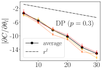
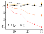
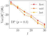
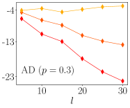
Figure 1: Mean and variance ($\log_{10}$ scale) of the magnitude of the cost function gradient for depolarizing (left) and amplitude-damping (right) channels with noise probability $p=0.3$ as a function of layers. Error bars in the upper plots represent the range between the maximum and minimum values.

Fig. 1 illustrates the magnitude of the cost function gradient (on a logarithmic scale) as a function of layers of the VQAs. Mean values (variances) are plotted in the top (bottom) two plots. Plots on the left (right) correspond to VQAs under depolarizing noise (amplitude-damping noise), both with a noise probability of $p=0.3$. We specifically present three angles corresponding to the initial, middle, and final layers of the VQA to emphasize their distinct behaviors. Additionally, the dot-dashed black line, denoted as $r^{l}$, is in proportion to the bound derived in Eq. 63 for the unital case. The solid black line is the numerical average over the three angles shown.

Under unital, depolarizing noise (upper and lower left), both the mean and variance of the gradient magnitude exhibit an exponential decay with an increasing number of layers. The error bars displayed in the upper plots represent the range between the maximum and minimum values. This suggests that all simulated mean values remain within the predicted bound. The observed behavior remains consistent irrespective of the specific layer within the VQA from which these angles were selected. The theoretical upper bound (dot-dashed line) is rather loose but consistent with the numerical results.

Under amplitude-damping noise (upper and lower right), distinct behaviors are observed among the three angles. The mean value of the magnitude of the gradient increases as the angle approaches the end of the VQA. The angle selected from the final layer consistently demonstrates a nearly constant gradient magnitude and violates the bound in Eq. 63, consistent with 3 and as anticipated in our theoretical analysis that angles within the terminal layers of the VQA circuit under non-unital noise may evade the NIBP.

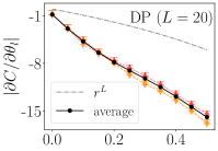
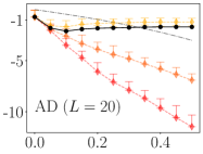
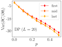
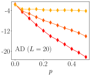
Figure 2: Mean and variance ($\log_{10}$ scale) of the magnitude of the cost function gradient for depolarizing (left) and amplitude-damping (right) channels as a function of noise probability $p$ in a VQA with 20 layers. Error bars in the upper plots represent the range between the maximum and minimum values.

Fig. 2 depicts an alternative view of Eq. 63, where the magnitude of the gradient is plotted as a function of the noise probability. The total number of layers in the VQA is fixed at $L=20$. The noise probability is varied from $p=0$ to $p=0.5$, corresponding to decreasing the parameter $r$ in Eq. 63. The behavior seen in Fig. 2 is similar to Fig. 1, where the magnitude of the gradient fully respects the derived bound only under depolarizing noise.

By fixing the noise probability and varying the number of layers (Fig. 1) or fixing the number of layers and varying the noise probability (Fig. 2), our simulations consistently demonstrate that Eq. 63 is well-respected in VQAs under unital noise and violated in VQAs under non-unital noise. This observation aligns with our theoretical predictions in 2 and 3. For a numerical examination of the standard (noise-free) BP, see Appendix F.

VI.2 Cost function behavior

Our results indicate that unital noise is subject to both NIBP and other forms of BP, and that, conversely, non-unital noise may potentially evade NIBP despite experiencing a comparable degree of other BPs. The primary question within the framework of VQA pertains to its efficacy in determining the ground state of a specific Hamiltonian. Consequently, in practical applications where the presence of noise is inevitable, the central concern revolves around identifying the type of noise that is comparatively less detrimental.

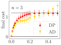
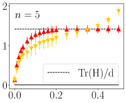
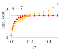
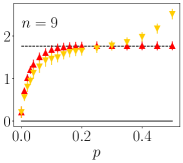
Figure 3: Final cost function averaged over $50$ random $n$-qubit Hamiltonians with zero ground state energy under depolarizing (red up-triangles) and amplitude-damping (yellow down-triangles) channels as a function of noise probability $p$ using VQA with $L=5$ layers. The solid black line at zero denotes the true minimum of the Hamiltonians used in this simulation. The error bars are the standard deviation of the final cost. The dashed black line is the predicted NIFP value in the large circuit depth limit in the unital case, Eq. 52.

To address this question, we determined the final cost function obtained by VQA circuits when subjected to unital and non-unital noise channels. The result displayed in Fig. 3 was achieved through the training of circuits responsible for generating the results illustrated in Figs. 1 and 2, showing the average of the instances for $n$-qubit Hamiltonians for $n=3,5,7$, and $9$ as a function of noise probability $p$.

The most obvious result from these simulations is that noise has a rapidly increasing, strongly detrimental effect: the final cost function rises rapidly from its optimal value of zero as soon as noise is introduced, whether unital or non-unital. Note that additionally, even at $p=0$, the final cost is greater than zero for $n\geq 5$ in our simulations, suggesting the effect of BPs.

The difference between unital and non-unital noise is small within the low-noise regime. The non-unital case exhibits a slightly better performance for small $p$, until reaching a crossover point typically observed within the range of $p=0.15-0.3$ (depending on $n$). However, a notable divergence in their behavior becomes evident as the probability of noise increases. In the case of depolarizing noise, the cost function flattens out at approximately $p=0.2$, whereas the cost function continues to rise when subjected to amplitude-damping noise, accelerating around $p=0.3$. This observation seems consistent with our NIFP result, where the cost function concentrates on a fixed point that is noise-independent in the unital case but noise-dependent in the non-unital case [Eq. 51]. Indeed, the final cost function value precisely matches the theoretically predicted $\mathrm{Tr}(H)/d$ in the unital case [Eq. 52].

Note that the theoretical prediction is concerned with the large $L$ limit, not large $p$. However, while the simulations in Fig. 3 are for fixed $L=5$, increasing $p$ at fixed $L$ is tantamount to increasing $L$ at fixed $p$, as is clear from Eq. 50a, where the factor $q^{L}$ is responsible for the NIFP, and $q$ is the contractivity factor, which is, of course, monotonic in $p$.

VII Conclusions

This work expands the study of NIBPs to incorporate arbitrary unital and single-qubit non-unital noise. Using a generalization of the parameter shift rule that includes noise, we have derived upper bounds for the scaling of the magnitude of the cost function gradient with respect to circuit width $n$, circuit depth $L$, and noise strength. In the unital case, we have shown that the onset of an NIBP occurs already for circuits of logarithmic depth (2), thereby tightening earlier bounds. In contrast, in the single-qubit non-unital case, we have shown that VQA circuits need not necessarily exhibit an NIBP. This is true, in particular, when a constant number of final layers in a VQA circuit are subject to non-unital noise (3).

We found that both unital and non-unital circuits exhibit a phenomenon we call a noise-induced fixed point (NIFP), whereby the cost function concentrates on a fixed value for circuits of greater than logarithmic depth. In the unital case, this is given by the expectation value of the problem Hamiltonian with respect to the fully mixed state [Eq. 52], but in the non-unital case, the fixed value is determined by the parameters of the noise channel as well [Eq. 51].

Our results are validated with numerical simulations for the depolarizing and amplitude-damping channels.

Overall, our work shows that NIBPs present a significant challenge for VQAs, even after mitigation of the standard (noiseless) BP problem. A combination of error suppression, mitigation, and correction methods will be necessary to realize the promise of VQAs, just as is the case for other quantum algorithms running on noisy quantum computers.

Appendix A Proof of Eq. 10

Using the purity condition $P\equiv\mathrm{Tr}\rho^{2}\leq 1$ in Eq. 9, we also have

$$1 \geq P=\mathrm{Tr}\left[\left(\frac{1}{d}I+\boldsymbol{F}\cdot\boldsymbol{v}\right)^{2}\right]$$ (93a)

$$=\frac{1}{d}+\sum_{i,j=1}^{M}\mathrm{Tr}(F_{i}F_{j})v_{i}v_{j}=\frac{1}{d}+\|\boldsymbol{v}\|^{2}\ ,$$ (93b)

i.e., $\|\boldsymbol{v}\|=\sqrt{P-1/d}$, and Eq. 10 follows.

Appendix B Proof of Eqs. 14 and 13

We use the Einstein summation convention for repeated indices. Using $\rho^{\prime}=\mathcal{N}(\rho)=K_{\alpha}\rho K_{\alpha}^{\dagger}$ and the expansion $\rho=\frac{1}{{d}}I+v_{i}F_{i}$, we have:

$$\frac{1}{{d}}I+v_{i}^{\prime}F_{i} =K_{\alpha}(\frac{1}{{d}}I+v_{i}F_{i})K_{\alpha}^{\dagger}$$ (94)

$$v_{i}^{\prime}F_{i} =\ (\frac{1}{{d}}K_{\alpha}K_{\alpha}^{\dagger}+v_{i}K_{\alpha}F_{i}K_{\alpha}^{\dagger})-\frac{1}{{d}}I$$

$$v_{i}^{\prime}\mathrm{Tr}[F_{j}F_{i}] =\frac{1}{{d}}\mathrm{Tr}[F_{j}K_{\alpha}K_{\alpha}^{\dagger}]+v_{i}\mathrm{Tr}[F_{j}K_{\alpha}F_{i}K_{\alpha}^{\dagger}]$$

$$v_{j}^{\prime} =\frac{1}{{d}}\mathrm{Tr}[F_{j}K_{\alpha}K_{\alpha}^{\dagger}]+v_{i}\mathrm{Tr}[F_{j}K_{\alpha}F_{i}K_{\alpha}^{\dagger}]$$

$$=c_{j}+M_{ji}v_{i}.$$

Eqs. 14 and 13 now follows from Eq. 94.

Appendix C Proof of 1

The $p$-norm of a matrix $A$ is defined as $\|A\|_{p}=\mathrm{Tr}(|A|^{p})^{1/p}=\sum_{i}(\lambda_{i}^{p})^{1/p}$, where $\lambda_{i}$ are the singular values of $A$, i.e., the eigenvalues of $|A|=\sqrt{A^{\dagger}A}$. The matrix Hölder inequality states that for $1\leq a,b\leq\infty$ and $\frac{1}{a}+\frac{1}{b}=1$ [59, 60] :

$$\langle A,B\rangle\leq\|A\|_{a}\|B\|_{b}.$$ (95)

An important special case for our purposes is $a=b=2$, i.e.:

$$\langle A,B\rangle\leq\sqrt{\langle A,A\rangle\langle B,B\rangle},$$ (96)

which is just the Cauchy-Schwarz inequality for matrices.

Any linear map $\Psi:\mathcal{B}(\mathcal{H})\mapsto\mathcal{B}(\mathcal{H})$ on operators $X\in\mathcal{B}(\mathcal{H})$ can be written as $\Psi(X)=\sum_{\alpha}E_{\alpha}XE_{\alpha}^{\prime{\dagger}}$, where $\{E_{\alpha},E^{\prime}_{\alpha}\}\in\mathcal{B}(\mathcal{H})$. Its Hermitian conjugate

$$\langle\Psi^{\dagger}(X),Y\rangle=\langle X,\Psi(Y)\rangle,$$ (97)

can be written explicitly as $\Psi^{\dagger}(X)=\sum_{\alpha}E_{\alpha}^{\dagger}XE_{\alpha}^{\prime}$ [61].

Therefore, if $\mathcal{N}=\{K_{\alpha}\}$ is a unital CPTP map, then so is $\mathcal{N}^{\dagger}$. The reason is that if $\mathcal{N}$ is unital then $\mathcal{N}(X)=\sum_{\alpha}K_{\alpha}XK_{\alpha}^{\dagger}$ and $\sum_{\alpha}K_{\alpha}K^{\dagger}_{\alpha}=\sum_{\alpha}K_{\alpha}^{\dagger}K_{\alpha}=I$. Thus $\mathcal{N}^{\dagger}(X)=\sum_{\alpha}K^{\dagger}_{\alpha}XK_{\alpha}$ has Kraus operators $\{L_{\alpha}=K_{\alpha}^{\dagger}\}$, and it immediately follows that $\sum_{\alpha}L^{\dagger}_{\alpha}L_{\alpha}=\sum_{\alpha}L_{\alpha}L^{\dagger}_{\alpha}=I$, i.e., also $\mathcal{N}^{\dagger}$ is a unital CPTP map.

Proof.

Consider $\rho\in\mathcal{B}_{+}(\mathcal{H})$ and let $P=\mathrm{Tr}(\rho^{2})=\langle\rho,\rho\rangle$ denote its purity. The purity $P^{\prime}$ of $\rho^{(1)}=\mathcal{N}(\rho)\equiv\mathcal{N}^{(0)}(\rho)$ can be written as:

$$P^{(1)} =\langle\rho^{(1)},\rho^{(1)}\rangle=\langle\mathcal{N}(\rho),\mathcal{N}(\rho)\rangle=\langle\rho,\mathcal{N}^{\dagger}[\mathcal{N}(\rho)]\rangle$$ (98a)

$$=\langle\rho,\mathcal{N}^{(1)}(\rho)\rangle\ ,$$ (98b)

where in the third equality we used Eq. 97. Here, $\mathcal{N}^{(1)}\equiv\mathcal{N}^{(0){\dagger}}\circ\mathcal{N}^{(0)}$ is the composition of two CPTP maps, so $\mathcal{N}^{(1)}$ is itself a CPTP map. Thus $\rho^{(2)}=\mathcal{N}^{(1)}(\rho)$ is a quantum state [i.e., $\rho^{(2)}\in\mathcal{B}_{+}(\mathcal{H})$].

Define $\forall n\geq 1$ a sequence of quantum maps $\mathcal{N}^{(n+1)}\equiv\mathcal{N}^{(n){\dagger}}\circ\mathcal{N}^{(n)}$, purities $P^{(n)}=\langle\rho^{(n)},\rho^{(n)}\rangle$, and states $\rho^{(n+1)}=\mathcal{N}^{(n)}(\rho)$. Then, using the Cauchy-Schwarz inequality for $n\geq 1$:

$$P^{(n)} =\langle\mathcal{N}^{(n-1)}(\rho),\mathcal{N}^{(n-1)}(\rho)\rangle=\langle\rho,\mathcal{N}^{(n)}(\rho)\rangle$$ (99a)

$$\leq\langle\rho,\rho\rangle^{1/2}\langle\rho^{(n+1)},\rho^{(n+1)}\rangle^{1/2}$$ (99b)

$$=P^{1/2}(P^{(n+1)})^{1/2}\ ,$$ (99c)

Expanding this recursion, we obtain:

$$P^{(1)}\leq P^{1/2}P^{1/4}\cdots P^{1/2^{n}}(P^{(n+1)})^{1/2^{n}}\ .$$ (100)

The purity is lower bounded by that of the fully mixed state $I/d$, where $d=\dim{\mathcal{H}}$: $P(I/d)=\mathrm{Tr}[(I/d)^{2}]=1/d$. Therefore $\forall n,d$ we have $1/d\leq P^{(n+1)}\leq 1$ and hence $\lim_{n\to\infty}(P^{(n+1)})^{1/2^{n}}=1$. Thus, upon taking the limit $n\to\infty$ of Eq. 100 we obtain:

$$P^{\prime}=P^{(1)}\leq P^{\sum_{n=1}^{\infty}2^{-n}}=P\ .$$ (101)

Equality in Eq. 99b holds iff $\mathcal{N}^{(n)}(\rho)=\rho$ $\forall n$, i.e., $\mathcal{N}^{(n)}=\mathcal{I}$, which means that in particular, after setting $n=1$, $\mathcal{N}^{(0){\dagger}}\circ\mathcal{N}^{(0)}=\mathcal{I}$, so that by definition $\mathcal{N}^{(0)}=\mathcal{N}$ must be a unitary superoperator: $\mathcal{N}(\rho)=\mathcal{U}(\rho)=U\rho U^{\dagger}$, where $U$ is unitary. ∎

Appendix D Proof of 3

Proof.

Note that Eq. 10 is a necessary condition on $\boldsymbol{v}$ in order for the coherence vector to represent a valid (positive semi-definite) density matrix via Eq. 9. It is also sufficient for $d=2$, but in dimensions $d>2$ additional conditions must be imposed for positive semi-definiteness [62]. For this reason, the proof of Eqs. 17a and 17b hold for arbitrary $d$, but the proof of Eqs. 17c, 17d and 17e holds for qubits only, i.e., it requires $d=2$. Indeed, using certain advanced results on Schatten $p$-norms, non-unital maps were shown to be non-contractive for $d\geq 3$ and contractive for $d=2$ [63]. The proof we give below uses only fairly elementary ideas and tools.

To prove Eq. 17a we use Eq. 14b to write $c_{i}=\frac{1}{{d}}\langle F_{i},X\rangle$ $\forall i\in\{1,\dots,d^{2}-1\}$, where $X=\sum_{\alpha}K_{\alpha}K_{\alpha}^{\dagger}$. In order for all the $c_{i}$ to vanish, $X$ must be simultaneously orthogonal to the entire basis. It follows that $X\propto I$, which is a contradiction since $\mathcal{N}$ is not unital. Hence $\boldsymbol{c}\neq\boldsymbol{0}$.

To prove Eq. 17b note that

$$\|\boldsymbol{v}^{\prime}\|=\|M\boldsymbol{v}+\boldsymbol{c}\|\leq\sqrt{1-1/d}<1\ \ \forall\boldsymbol{v}\text{ s.t. }\|\boldsymbol{v}\|\leq\sqrt{1-1/d},$$ (102)

where we used Eq. 10. This must hold in particular for the maximally mixed state, i.e., when $\boldsymbol{v}=\boldsymbol{0}$. Hence, $\|\boldsymbol{c}\|<1$.

To prove Eq. 17c, let $\boldsymbol{w}$ be the eigenvector of $S$ with the largest eigenvalue $\lambda_{1}\equiv\sigma_{\max}(M)$, i.e., $S\boldsymbol{w}=\lambda_{1}\boldsymbol{w}$. Normalizing $\boldsymbol{w}$ so that $\boldsymbol{v}=\frac{\sqrt{1-1/d}}{\|\boldsymbol{w}\|}\boldsymbol{w}$, we have $\|\boldsymbol{v}\|=\sqrt{1-1/d}<1$, and $\boldsymbol{v}$ is a pure state in $\mathcal{H}=\mathbb{C}^{d}$ that is also an eigenvector of $S$ with eigenvalue $\lambda_{1}$. Then $\|OS(\pm\boldsymbol{v})\|=\|S\boldsymbol{v}\|=\lambda_{1}\|\boldsymbol{v}\|=\lambda_{1}\sqrt{1-1/d}$. Using Eq. 102 and $M=OS$, we have:

$$1-1/d\geq\|\pm M\boldsymbol{v}+\boldsymbol{c}\|^{2}=(1-1/d)\lambda_{1}^{2}+\|\boldsymbol{c}\|^{2}\pm 2(M\boldsymbol{v})\cdot\boldsymbol{c}.$$ (103)

Now assume that $\lambda_{1}\geq 1$; this means that $\|\boldsymbol{c}\|^{2}\pm 2(M\boldsymbol{v})\cdot\boldsymbol{c}\leq 0$. Combining the two cases we thus have

$$2M\boldsymbol{v}\cdot\boldsymbol{c}\geq\|\boldsymbol{c}\|^{2}\quad\text{and}\quad 2M\boldsymbol{v}\cdot\boldsymbol{c}\leq-\|\boldsymbol{c}\|^{2}$$ (104)

which can only be true if $\boldsymbol{c}=\boldsymbol{0}$. Since we are considering the non-unital map where $\boldsymbol{c}\neq\boldsymbol{0}$, by contradiction, $\lambda_{1}<1$.

Finally, since $\|M\boldsymbol{v}\|=\|OS\boldsymbol{v}\|=\|S\boldsymbol{v}\|\leq\lambda_{1}\|\boldsymbol{v}\|$ and $\lambda_{1}<1$, it follows that $\|M\boldsymbol{v}\|<\|\boldsymbol{v}\|$, which proves Eq. 17d.

To prove Eq. 17e, let $\boldsymbol{u}=M\boldsymbol{v}$ and decompose it into the component parallel to $\boldsymbol{c}$ and the orthogonal component:

$$\boldsymbol{u}=u_{\|}\hat{\boldsymbol{c}}+u_{\bot}\hat{\boldsymbol{c}}^{\bot},$$ (105)

where $\hat{\boldsymbol{c}}=\boldsymbol{c}/\|\boldsymbol{c}\|$ and $\hat{\boldsymbol{c}}^{\bot}$ are orthonormal. Using $\|\boldsymbol{v}^{\prime}\|\leq\sqrt{1-1/d}$, we have

$$\|\boldsymbol{v}^{\prime}\|=\|\boldsymbol{u}+\boldsymbol{c}\|=\|(u_{\|}+\|\boldsymbol{c}\|)\hat{\boldsymbol{c}}+u_{\bot}\hat{\boldsymbol{c}}^{\bot}\|\leq\sqrt{1-1/d}.$$ (106)

This must be true $\forall\boldsymbol{u}$, including when $u_{\bot}=0$, where we have $|u_{\|}+\|\boldsymbol{c}\||\leq\sqrt{1-1/d}$. Assume that $u_{\|}\geq 0$; then $|u_{\|}+\|\boldsymbol{c}\||=|u_{\|}|+\|\boldsymbol{c}\|$ and $|u_{\|}|=\|M\boldsymbol{v}\|\geq\lambda_{2}\|\boldsymbol{v}\|$, where $\lambda_{2}\equiv\sigma_{\min}(M)$ is the smallest eigenvalue of $S$. The bound holds for any $\|\boldsymbol{v}\|\leq\sqrt{1-1/d}$, in particular when the state is pure, for which $\|\boldsymbol{v}\|=\sqrt{1-1/d}$. Combining the above bounds, we obtain:

$$\lambda_{2}\|\boldsymbol{v}\|+\|\boldsymbol{c}\| \leq\lambda_{2}\sqrt{1-1/d}+\|\boldsymbol{c}\|$$ (107a)

$$\leq|u_{\|}|+\|\boldsymbol{c}\|=|u_{\|}+\|\boldsymbol{c}\||$$ (107b)

$$\leq\|(u_{\|}+\|\boldsymbol{c}\|)\hat{\boldsymbol{c}}+u_{\bot}\hat{\boldsymbol{c}}^{\bot}\|\leq\sqrt{1-1/d}\ ,$$ (107c)

where in the last two lines $\boldsymbol{u}=M\boldsymbol{v}$ and we took $\boldsymbol{v}$ to be pure. We thus arrive at:

$$\sigma_{\min}(M)+\|\boldsymbol{c}\|/\sqrt{1-1/d}\leq 1.$$ (108)

If $u_{\|}<0$, then replacing $\boldsymbol{v}$ by $-\boldsymbol{v}$ makes $u_{\|}>0$ (since $u_{\|}=\hat{\boldsymbol{c}}\cdot M\boldsymbol{v}$). This replacement does not change anything about Eq. 107 or the argument that leads to it; hence, the bound in Eq. 108 still holds. ∎

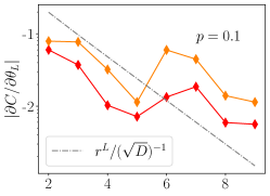
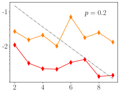
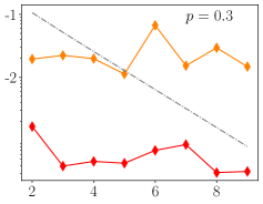
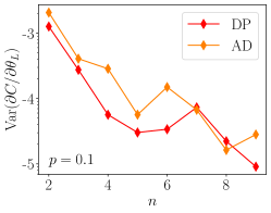
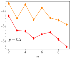
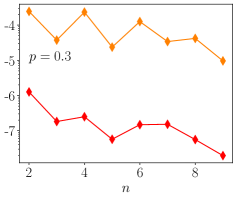
Figure 4: Magnitude and variance of the gradient of the cost functions for depolarizing (left) and amplitude-damping (right) channels as a function of the number of qubits for noise probabilities $p=0.1$, $0.2$, and $0.3$ in the leftmost, middle, and rightmost plots, respectively. Error bars in the top three plots represent the range of the values.

Appendix E Proof of Eq. 34

Using Eq. 20c, the noisy cost function is:

$$C^{\prime}(\boldsymbol{\theta})=\mathrm{Tr}[\tilde{H}\mathcal{V}(\theta_{\mu})(\tilde{\rho})]$$ (109a)

$$\quad=p_{j}\mathrm{Tr}[\tilde{H}\mathcal{U}(\theta_{\mu})(\tilde{\rho})]+\sum_{k\neq j}p_{k}\mathrm{Tr}[\tilde{H}\mathcal{V}^{\prime}_{k}(\theta_{\mu})(\tilde{\rho})].$$ (109b)

Using Eq. 22, we now have:

$$\frac{\partial C^{\prime}(\boldsymbol{\theta})}{\partial\theta_{\mu}}=p_{j}\frac{\partial C(\boldsymbol{\theta})}{\partial\theta_{\mu}}-\frac{i}{2}\sum_{k\neq j}p_{k}\mathrm{Tr}[\tilde{H}\mathcal{V}^{\prime}(\theta_{\mu})([P_{k},\tilde{\rho}])]$$ (110a)

$$=p_{j}\frac{\partial C(\boldsymbol{\theta})}{\partial\theta_{\mu}}+\frac{1}{2}\sum_{k\neq j}p_{k}\mathrm{Tr}[\tilde{H}\mathcal{V}^{\prime}(\theta_{\mu})\times$$ (110b)

$$\qquad\qquad\qquad\qquad\left(\mathcal{U}_{k}\left(\frac{\pi}{2}\right)(\tilde{\rho})-\mathcal{U}_{k}\left(-\frac{\pi}{2}\right)(\tilde{\rho})\right)]$$

$$=p_{j}\frac{\partial C(\boldsymbol{\theta})}{\partial\theta_{\mu}}+\frac{1}{2}\sum_{k\neq j}p_{k}\mathrm{Tr}(\tilde{H}\tilde{\xi}_{k}),$$ (110c)

where $\tilde{\xi}_{k}=\tilde{\rho}^{+}_{k}-\tilde{\rho}^{-}_{k}$ and $\tilde{\rho}_{k}^{\pm}=\mathcal{V}^{\prime}(\theta_{\mu})\mathcal{U}_{k}\left(\pm\frac{\pi}{2}\right)(\tilde{\rho})$. Thus,

$$\left|\frac{\partial C^{\prime}(\boldsymbol{\theta})}{\partial\theta_{\mu}}\right|\leq p_{j(\mu)}\left|\frac{\partial C(\boldsymbol{\theta})}{\partial\theta_{\mu}}\right|+\frac{1}{2}\sum_{k\neq j}p_{k(\mu)}|\tilde{\boldsymbol{w}}_{k(\mu)}\cdot\boldsymbol{h}|.$$ (111)

This directly yields the bound on the gradient given in Eq. 34.

Appendix F Upper bound dependence on circuit width

In Eq. 73, we considered the overlap of two vectors chosen at random, which suggests that the gradient of the cost function exhibits an inverse square root dependence on the dimensionality, denoted as $1/\sqrt{D}$ where $D=d^{2}-1=2^{2n}-1$ and $d$ is the Hilbert space dimension. This phenomenon was initially discussed in Ref. [24] and is the original (noise-free) barren plateau (BP). To rederive it, we follow the approach of Ref. [64].

Consider two normalized $D$-dimensional vectors $\boldsymbol{v}$ and $\boldsymbol{h}$, and choose each component of $\boldsymbol{h}$ uniformly from the surface of a normalized $D$-Ball. Two vectors $\boldsymbol{v}$ and $\boldsymbol{h}$ are orthogonal when $\boldsymbol{v}\cdot\boldsymbol{h}=0$. Using the summation convention, the expectation value of the inner product of $\boldsymbol{v}$ and $\boldsymbol{h}$ is $\mathbb{E}[\boldsymbol{v}\cdot\boldsymbol{h}]=\mathbb{E}[v_{i}h_{i}]=0$. The variance of the inner product of $\boldsymbol{v}$ and $\boldsymbol{h}$ is $\sigma^{2}[\boldsymbol{v}\cdot\boldsymbol{h}]=\mathbb{E}[v_{i}h_{i}v_{j}h_{j}]-\mathbb{E}[\boldsymbol{v}\cdot\boldsymbol{h}]^{2}=\frac{1}{D}$.

The Chernoff bound states that $\mathrm{Pr}(X>\epsilon)<\exp(-\frac{\epsilon^{2}}{\sigma[X]^{2}})$. Hence, $\mathrm{Pr}(|\boldsymbol{v}\cdot\boldsymbol{h}|>\epsilon)<e^{-D\epsilon^{2}}$. Applying this bound to Eq. 73, we have $\mathrm{Pr}\left(\left|\frac{\partial C(\boldsymbol{\theta})}{\partial\theta_{Lm}}\right|>\epsilon\right)<e^{-D\epsilon^{2}}$, where $D=2^{2n}-1$ for an $n$-qubit VQE. This result can be interpreted as stating that the cost function gradient is exponentially small in the number of qubits (circuit width) but not in the number of layers (circuit depth).

Next, we examine whether the dependence on circuit width can be observed in numerical simulations of the same type as discussed in Section VI. We again employ a set of $50$ randomly chosen $n$-qubit Hamiltonians, with $2\leq n\leq 9$. Fig. 4 shows the result of the simulation. As we explained, it is anticipated that the gradient magnitude will be proportional to $1/\sqrt{D}$. We emphasize that this does not constitute an upper bound for the magnitude; rather, it represents an excepted value obtained through averaging over a large number of randomly generated vectors.

The simulations we have conducted do not exhibit a discernible trend along the dashed-dotted gray line denoted as $1/\sqrt{D}$. Both depolarizing and amplitude-damping noise manifest analogous patterns. The magnitude of the gradient appears to remain relatively stable with respect to the number of qubits $n$ as the noise probability increases. This failure to observe the expected BP behavior is likely attributable to a combination of a small sample size of $50$ samples and $n$ being too small.