BECoTTA: Input-dependent Online Blending of Experts
for Continual Test-time Adaptation

Abstract

Continual Test Time Adaptation (CTTA) is required to adapt efficiently to continuous unseen domains while retaining previously learned knowledge. However, despite the progress of CTTA, forgetting-adaptation trade-offs and efficiency are still unexplored. Moreover, current CTTA scenarios assume only the disjoint situation, even though real-world domains are seamlessly changed. To tackle these challenges, this paper proposes BECoTTA, an input-dependent yet efficient framework for CTTA. We propose Mixture-of-Domain Low-rank Experts (MoDE) that contains two core components: (i) Domain-Adaptive Routing, which aids in selectively capturing the domain-adaptive knowledge with multiple domain routers, and (ii) Domain-Expert Synergy Loss to maximize the dependency between each domain and expert. We validate our method outperforms multiple CTTA scenarios including disjoint and gradual domain shits, while only requiring $\sim$98% fewer trainable parameters. We also provide analyses of our method, including the construction of experts, the effect of domain-adaptive experts, and visualizations.

1 Introduction

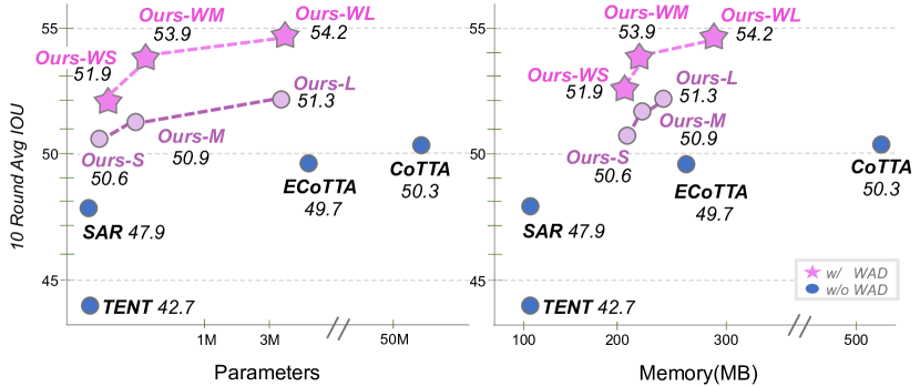
Figure 1: Our BECoTTA achieves superior performance and parameter/memory efficiency against strong CTTA baselines on the CDS-hard scenario. WAD represents the Weather-Augmented Dataset described in  Sec. 3.1

.

Test-Time Adaptation (TTA) (Wang et al., 2020; Niu et al., 2023; Wang et al., 2022a; Lim et al., 2023; Lee et al., 2023a) is a challenging task that aims to adapt the pre-trained model to new, unseen data at the time of inference, where the data distribution significantly differs from that of the source dataset. TTA approaches have become popular since they address the critical challenge of model robustness and flexibility in the face of new data.

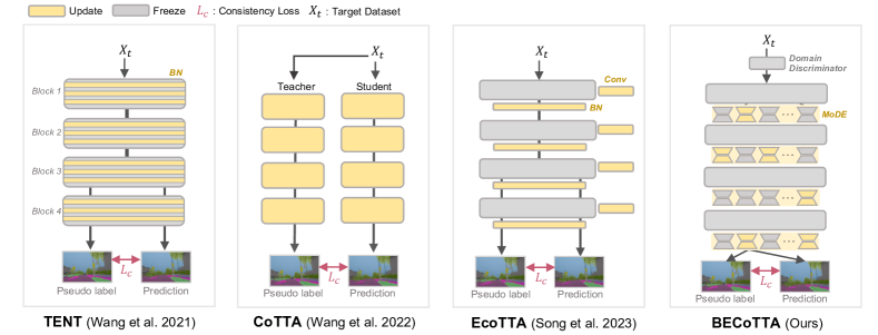
Figure 2: Comparison of TTA process with other SoTA models. We compare the existing models (Wang et al., 2020, 2022a; Song et al., 2023) and denote activated modules as yellow during CTTA process. In particular, CoTTA adopts the mean-teacher architecture and updates the entire model. TENT (Wang et al., 2020) and EcoTTA (Song et al., 2023) update a few parts of the model, however, they achieve suboptimal performance with forgetting. Meanwhile, our BECoTTA updates only MoDE layers for efficient and rapid adaptation while preserving previous knowledge.

Beyond the isolated transferability of traditional TTA approaches on the stationary target domain, Continual Test-Time Adaptation (CTTA) (Niu et al., 2023; Song et al., 2023; Lee et al., 2023a) has been increasingly investigated in recent years, whose goal is to continuously adapt to multiple unseen domains arriving in sequence. Solving the problem of CTTA is crucial because it is closely related to real-world scenarios. For example, let us assume that a vision model in an autonomous vehicle aims to understand road conditions and objects, including pedestrians, vehicles, traffic signs, etc. The agent will encounter different environments over time, according to the changes in the weather, time of the day, and location. Then, the model should rapidly and continuously adapt to these unseen environments while retaining the domain knowledge learned during adaptation as it may re-encounter prior domains in the future.

Therefore, continual TTA approaches need to address the following key challenges: (i) forgetting-adaptation trade-off: retaining previous domain knowledge while learning new domains often limits the model’s plasticity, hindering its ability to learn and adapt to new data, and (ii) computational efficiency: since CTTA models are often assumed to be embedded in edge devices, efficient adaptation is significant. However, as shown in Fig. 2, existing CTTA methods overlook computational efficiency by updating heavy teacher and student models (Wang et al., 2022a) or achieved suboptimal convergence due to updating only a few parts of modules (Wang et al., 2020; Niu et al., 2023; Gan et al., 2023; Gao et al., 2022b).

To tackle these critical issues, this paper proposes Input-dependent Online Blending of Experts for Continual Test-Time Adaptation (BECoTTA) by introducing a surprisingly efficient yet effective module, named Mixture-of-Domain Low-rank Experts (MoDE), atop each backbone block. Our BECoTTA method consists of two key components: (i) Domain Adaptive Routing and (ii) Domain-Expert Synergy Loss. We first propose Domain Adaptive Routing that aims to cluster lightweight low-rank experts (i.e., MoDE modules) with relevant domain knowledge. Next, based on the assignment of domain adaptive routers, we propose Domain-Expert Synergy Loss to maximize the mutual information between each domain and its corresponding expert. In the end, we facilitate cooperation and specialization among domain experts by ensuring strong dependencies. Our modular design allows for selective updates of multiple domain experts, ensuring the transfer of knowledge for each specific domain while preserving previously acquired knowledge. This approach also significantly improves memory and parameter efficiency through sparse updates.

Furthermore, existing CTTA scenarios assume a disjoint change of test domains, where the model encounters a static domain per time step, but do not consider a gradual shift of domains, which is more common in the real world (e.g., seamless weather change like cloudy $\rightarrow$ rainy or afternoon $\rightarrow$ night). To further consider this realistic scenario, we additionally propose Continual Gradual Shifts (CGS) benchmark for CTTA, where the domain gradually shifts over time based on domain-dependent sampling distribution, as illustrated in Fig. 3 top left. This scenario is more advanced than an existing CTTA problem as it demands the model to appropriately adapt each of the input instances, without relying on any implicit guidance from the dominant domain over a given time interval.

We compare our proposed method with strong baselines, including SAR (Niu et al., 2023), DePT (Gao et al., 2022b), VDP (Gan et al., 2023), and EcoTTA (Song et al., 2023), on multiple CTTA scenarios and our suggested CGS benchmark. Our BECoTTA achieves +2.1%p and +1.7%p IoU enhancement respectively on CDS-Hard and CDS-Easy scenarios, by utilizing 95% and 98% fewer parameters used by CoTTA (Wang et al., 2022a). In addition, for the WAD scenario where the source models were additionally pre-trained on the Weather-Augmented Datasets, our model consistently shows +16.8%p performance gain over EcoTTA, utilizing a similar number of parameters on the CDS-Hard scenario (Please see Fig. 2).

We summarize our contributions as threefold:

• We propose an efficient yet powerful CTTA method, named BECoTTA, which adapts to new domains effectively with minimal forgetting of the past domain knowledge, by transferring only beneficial representations from relevant experts.

• We introduce a new realistic CTTA benchmark, Continual Gradual Shifts (CGS) where the domain gradually shifts over time based on domain-dependent continuous sampling probabilities.

• We validate our BECoTTA on various driving scenarios, including three CTTA and one domain generalization, demonstrating the efficacy and efficiency against strong baselines, including TENT, EcoTTA, and SAR.

2 Related Works

Continual Test-Time Adaptation.

Continual Test-Time Adaptation (CTTA) (Wang et al., 2022a; Gan et al., 2023; Niu et al., 2023; Song et al., 2023) assumes that target domains are not fixed but change continuously in an online manner. TENT (Wang et al., 2020) is one of the pioneering works, which activates only BatchNorm layers to update trainable affine transform parameters. CoTTA (Wang et al., 2022a) introduces a teacher-student framework, generating pseudo labels from the teacher model and updating it using consistency loss. EcoTTA (Song et al., 2023) utilizes meta networks and self-distilled regularization while considering memory efficiency. DePT (Gao et al., 2022b) plugs visual prompts for efficiently adapting target domains and bootstraps the source representation. However, existing methods often suffer from subordinate convergence since they rely on a shared architecture for adapting test data without considering the correlation between different domains. On the other hand, our BECoTTA introduces a modularized MoE-based architecture where each expert captures domain-adaptive knowledge, and the model transfers only a few related experts for the adaptation of a new domain.

Moreover, recent works (Song et al., 2023; Niu et al., 2022; Lim et al., 2023; Choi et al., 2022a; Liu et al., 2021; Adachi et al., 2022; Jung et al., 2023; Lee et al., 2023b) allow for a slight warmup using the source dataset before deploying the model to CTTA scenario. In particular, TTA-COPE (Lee et al., 2023b) conducts pretraining with labeled source datasets in a supervised manner. EcoTTA (Song et al., 2023) also proceed warm-up to initialize their meta-network. Note that all of them are operationalized in source-free at test time and there is agreement that this setting adheres to the assumptions of CTTA.

Mixture-of-Experts.

Mixture-of-Experts (MoE) (Shazeer et al., 2017; Fedus et al., 2022; Zuo et al., 2021; Wang et al., 2022b) introduces $N$ parallel experts consisting of the feed-forward network with router modules, and sparsely activate a few experts based on their sampling policies. Adamix (Wang et al., 2022b) introduces efficient fine-tuning with Mixture-of-Adaptations structures to learn multiple views from different experts. THOR (Zuo et al., 2021) proposes a new stochastic routing function to prevent inefficiency with routers. Similarly, Meta DMoE (Zhong et al., 2022) adopts the MoE architecture as a teacher model and distills their knowledge to unlabeled target domains, but they do not consider continuous adaptation. In short, to the best of our knowledge, the feasibility of MoE structures is underestimated in the field of CTTA.

Blurry Scenario in Continual Learning.

Recently, a few continual learning appraoches (Koh et al., 2021; Bang et al., 2021, 2022; Aljundi et al., 2019) have discussed Blurry Continual Learning (Blurry-CL) to better reflect real-world scenarios, beyond the standard CL setting. Blurry-CL assumes that for each sequential task, a majority class exists, and other classes outside the majority class may also overlap and appear. The most renowned scenario setup is a Blurry-M (Aljundi et al., 2019), where the majority class occupies 100-M%, and the remaining classes are randomly composed of M%. While this benchmark handles an overlapping situation, it may not cover practical situations where the domain evolves gradually in CTTA. Therefore, we propose a new benchmark that simulates real-world continual TTA scenarios with a gradual change of domains over time.

3 Input-dependent Online Blending of Experts for Continual Test-time Adaptation

We first define the problem statement of Continual Test-Time Adaptation (CTTA) in Sec. 3.1. Next, we introduce a novel proposed CTTA method, BeCoTTA, containing Mixture-of-Domain Low-rank Experts (MoDE) and domain-expert synergy loss in Sec. 3.2. After that, we describe the overall optimization process during CTTA in Sec. 3.3.

3.1 Problem Statement

Continual Test-time Adaptation (CTTA) aims to adapt the pre-trained source model $\bm{f_{s}}$ to continuously changing target domains, as formulated to a task sequence $\bm{X_{t}}=\{X_{t}^{1},X_{t}^{2},..X_{t}^{c},\cdots\}$. The main assumption of CTTA includes two folds: (i) we should not access the source dataset after deploying model to the test time, and (ii) adaptation needs to be done online and in an unsupervised manner. For semantic segmentation tasks, the objective of CTTA is to predict the softmax output $\hat{y_{c}}=f_{c}(\bm{x}_{t}^{c})$ at target domain $c$. $\bm{x}_{t}^{c}$ is sampled from $X_{t}^{c}$, which will be represented $\bm{x}$ from the following sections for brevity.

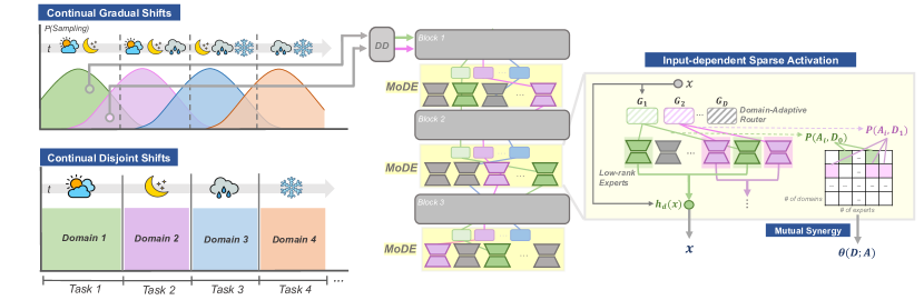
Figure 3: The overview of BECoTTA. We propose a novel CTTA framework for dynamic real-world scenarios, including disjoint and gradual shifts of domains. When the model receives a target domain input $\bm{x_{t}}$ at timestep $t$, the Domain Discriminator (DD) first estimates a pseudo domain label $d$. Based on the estimated pseudo labels, the domain router $G_{d}$ processes the input to specific experts containing domain-specific information via minimizing our proposed Domain-Expert Synergy Loss $\Theta(D;A)$. Finally, we obtain domain-adaptive representation $h_{d}(\bm{x})$, addressing downstream tasks in test-time.

Parameter Initialization for CTTA. Most CTTA methods use a pre-trained frozen backbone, which contains domain bias from the source domain. This bias impedes the effective transfer of domain-adaptive knowledge in continuous scenarios, due to the predominance of the source domain. To mitigate this limitation, we define the various candidate $D$ domains (e.g., brightness, darkness, blur) and apply the augmentation to the source domain similar to EcoTTA (Song et al., 2023) and DDA (Gao et al., 2022a), coined Weather-Augmented Dataset (WAD). For the augmentation, we utilize pre-trained style-transfer (Jiang et al., 2020) or simple transformations (Buslaev et al., 2020). Through WAD, we acquire domain-specific knowledge before deploying TTA. Note that this process is only done once when setting the source domain. More details are in the Appendix (Sec. D).

3.2 Mixture-of-Domain Low-rank Experts (MoDE)

We now introduce our new CTTA approach to efficiently capture the domain-adaptive representation via cooperation and specialization of multiple experts, dubbed Input-dependent Online Blending of Experts for Continual Test-Time Adaptation (BECoTTA). Our proposed BECoTTA employs Mixture of Domain low-rank Experts (MoDE) layers at the top of each block in the pre-trained ViT backbone.

The design of Low-rank Experts. For the efficient process during CTTA, we adopt the Sparse Mixture-of-Experts (SMoE) module with a top-k routing policy (Shazeer et al., 2017). Each MoE layer consists of the router $G$ and a set of $N$ lightweight experts, $A_{1}$, $A_{2}$, …, $A_{N}$, where each $A_{i}$ is parameterized by $\bm{W}_{i}^{down}\in\mathbb{R}^{dim\times r}$ and $\bm{W}_{i}^{up}\in\mathbb{R}^{r\times dim}$. Here, $r$ denotes the rank, and $dim$ denotes the embedding dimension of each ViT block. If the $A_{i}$ is activated, it maps the input $\bm{x}$ into the low dimensional space through the projection operation with $\bm{W}_{i}^{down}$. Next, after regularizing the features with a non-linear activation function $\sigma(\cdot)$, it recovers the features to the original dimension using $\bm{W}_{i}^{up}$:

$$A_{i}=\sigma(\bm{x}\bm{W}_{i}^{down})\bm{W}_{i}^{up}.$$ (1)

Domain-Adaptive Routing. Since each domain contains different key features, transferring them to other domains is not always advantageous. However, recent CTTA approaches, such as TENT (Wang et al., 2020), SAR (Niu et al., 2023), and EcoTTA (Song et al., 2023), continuously adapt to new domains by updating trainable parameters in a domain-agnostic manner. This means that they update the equivalent set of parameters for adapting a variety of different domains over time, which restricts the ability to learn fine-grained features for each domain due to the negative interference from irrelevant domain knowledge. In addition, adjusting all parameters for new domains causes the model to forget the past domain information, struggling to retain domain representations learned before when encountering the same or similar domains again.

Therefore, as shown in Fig. 3, we introduce $D$ independent domain-wise routers $G_{1}$, $G_{2}$..$G_{D}$ to loosely cluster experts of the model with similar domain knowledge by selecting $K$ experts per layer. We note that our modular architecture containing multiple parameter-efficient experts allows the model to efficiently yet effectively capture domain-adaptive representations while avoiding negative interference from less relevant features and preventing unintentional shifts of previously learned domains. Each router $G_{d}$ for domain $d$ is parameterized by $\bm{W}^{g}_{d}\in\mathbb{R}^{dim\times N}$ and $\bm{W}^{noise}_{d}\in\mathbb{R}^{dim\times N}$, and operates as follows:

$$P_{d}(\bm{x})=\bm{x}\bm{W}^{g}_{d}+N\left(0,1\right)\cdot\text{\text{Softplus}}\left(\bm{x}\bm{W}^{noise}_{d}\right),$$ (2)

$$G_{d}(\bm{x})=\text{Softmax}\left(TopK\left(P_{d}(\bm{x})\right)\right).$$ (3)

Based on the $G_{d}(\bm{x})$, we selectively update the activated experts associated with the specific domain, inherently isolating them from irrelevant domain knowledge while adapting new ones. In the end, the output of MoDE layer $h_{d}(x)$ aggregate the domain-adaptive features as follows:

$$h_{d}(\bm{x})=\sum_{i=1}^{N}G_{d}^{i}(\bm{x})\cdot A_{i}.$$ (4)

This trainable clustering approach allows the model to activate its own set of experts, who are specialized in specific domain knowledge. Moreover, our multi-router-based design accelerates adaptation to the current domain, avoiding interference from knowledge transfer of unrelated domain features. Finally, we perform the skip connection operation with original input $\bm{x}$: $\bm{x}\leftarrow\bm{x}+h_{d}(\bm{x})$.

We emphasize that the pre-defined $D$ domains do not need to match CTTA target domains. The main role of the WAD is to differentiate routers so the model can aggregate different visual features during continual TTA phases. Our BECoTTA is able to update relevant MODE modules with respect to the inputs and consistently achieves competitive performance even when the WAD and target domains are disjoint. (Please refer to Tab. 6 for details.)

Maximizing Domain-Expert Synergy. In cases where some domains share similar visual contexts (e.g., snow and fog), collaboration between domain experts can be beneficial. On the other hand, for unique scenes like night, it is advantageous to isolate domain features from others. That is, ensuring strong interdependence among various domains and experts is essential. To this end, we propose Domain-Expert Synergy loss based on the output from domain-adaptive routers. Let us consider $G_{d}^{i}(\bm{x})$ is assignment weight with specific domain $d$ from the $i$-th expert $A_{i}$, then $P(A_{i}|d)$ is obtained from all of the experts and domains in each MoDE layer. Then, we calculate $P(A_{i},d)$ using the Bayes’ theorem:

$$P(A_{i},d)=P(A_{i}|d)\cdot P(d),$$ (5)

where $P(d)$ represents the frequency of occurrence in domain $d$. Since it is infeasible to define $P(d)$ in most real-world scenarios, we assume the uniform distribution over $P(d)$. Next, to measure and maximize the mutual dependency among domains and experts, we adopt the probability modeling as a double sum:

$$\Theta(D;A)=\sum_{d}^{D}\sum_{i}^{N}P(A_{i},d)\cdot\log\frac{P(A_{i},d)}{P(A_{i})P(d)}.$$ (6)

Maximizing $P(A_{i},d)\log P(A_{i},d)$ leads the model to obtain a sharper conditional distribution of $P(A_{i}|d)$, facilitating the dependency between domains and experts. That is, our domain-adaptive experts can be further specialized in their respective domains and collaborate with others who share their domain knowledge.

3.3 Continual Test-time Adaptation Process

Model Initialization. We initialize our BECoTTA and baselines into two different settings: random initialization and post-pre-training with a Weather-Augmented Dataset (WAD). Following recent trends in CTTA (Song et al., 2023; Niu et al., 2022; Lim et al., 2023; Choi et al., 2022a; Liu et al., 2021; Adachi et al., 2022; Jung et al., 2023) and for a fair comparison, we perform a short pre-training for trainable parameters in models before deploying them to the CTTA problems. (Please refer to Tab. 1). For the pre-training initialization, we first build the WAD with $D$ domains. Next, we introduce a Domain Discriminator (DD) as the auxiliary head. It consists of lightweight CNN layers and is trained on WAD to classify the pre-defined $D$ domains. This helps the model distinguish between different domains and classify each test-time image input accordingly during test-time adaptation on a sequence of unseen domains. Then, we update MoDE layers and DD for only a small number of epochs. The total initialization loss $L_{init}$ is formulated below. Except for original cross-entropy loss $L_{seg}$ for semantic segmentation, we include cross-entropy loss $L_{disc}$ for DD, and domain-expert synergy loss $\Theta(D;A)$:

$$L_{init}=L_{seg}+\lambda_{disc}L_{disc}-\lambda_{s}\Theta(D;A)$$ (7)

where $\lambda_{disc}$, $\lambda_{s}$ denotes the balance term for each loss.

Source-free TTA with MoDE. Building upon the initialized MoDE, we deploy our BECoTTA to real-world continual scenarios. Note that we do not access any source dataset after the deployment, maintaining the source-free manner in the test time as other prior works. In the source-free TTA, we only activated MoDE layers to transfer the target domain knowledge efficiently. Utilizing the frozen DD trained at initialization, we get the pseudo domain label $d$ per each domain-agnostic target image $x_{t}^{c}$. Afterward, according to $d$, we initially assign the domain-wise router and proceed with the aggregation of domain-adaptive experts. This approach ensures that our BECoTTA maintains input dependency, even within a dynamic continual scenario.

Following the preliminary works (Wang et al., 2020; Song et al., 2023; Niu et al., 2022), we adopt the entropy minimization using $H(\hat{y_{c}})=-\sum p(\hat{y_{c}})\cdot\log p(\hat{y_{c}})$. To prevent forgetting and error accumulation, we conduct entropy filtering based on the confidence of the pseudo labels. Therefore, the entropy-based loss $L_{tta}$ is as follows:

$$L_{tta}=\mathds{1}_{\{{H(\hat{y_{c}})<\kappa}\}}\cdot H(\hat{y_{c}}),$$ (8)

where $\hat{y_{c}}$ is the output prediction in the current target domain stage $c$, $\kappa$ is the pre-defined entropy threshold, and $\mathds{1}\{\cdot\}$ denotes an indicator function.

4 Experiments

4.1 Data Setup

Table 1: Results on CDS-Hard (imbalanced weather & area shifts). We devise a novel scenario encompassing imbalanced weather and area shifts. We present performance results for both w/o WAD and w/ WAD across the overall baselines. We report $S$, $M$, and $L$ versions for our BECoTTA based on the number of parameters.

Round			1						10						$\Delta$	Parameter
Init	Method	Init update	B-Clear	A-Fog	A-Night	A-Snow	B-Overcast	Mean	B-clear	A-Fog	A-Night	A-Snow	B-Overcast	Mean
	Source only	-	41.0	64.4	33.4	54.3	46.3	47.9	41.0	64.4	33.4	54.3	46.3	47.9	+0.0	-
	CoTTA (Wang et al., 2022a)	-	43.3	67.3	34.8	56.9	48.8	50.2	43.3	67.3	34.8	56.9	48.8	50.2	+0.0	54.72M
	TENT (Wang et al., 2020)	-	41.1	64.9	33.2	54.3	46.3	47.9	30.9	51.5	20.4	37.0	33.0	34.6	-13.3	0.02M
w/o WAD	SAR (Niu et al., 2023)	-	41.0	64.5	33.4	54.5	46.6	48.0	41.3	64.3	31.6	54.2	46.6	47.6	-0.4	0.02M
	EcoTTA (Song et al., 2023)	MetaNet	44.1	69.6	35.3	58.2	49.6	51.3	41.9	66.1	31.5	55.3	46.2	48.2	-3.1	3.46M
	BECoTTA (Ours)-S	MoDE	42.9	68.5	35.0	57.2	47.8	50.5	43.0	68.5	35.1	57.3	48.8	50.7	+0.1	0.09M
	BECoTTA (Ours)-M	MoDE	43.8	68.8	34.9	57.9	49.2	50.9	43.7	68.8	34.5	57.9	49.2	50.9	+0.0	0.63M
	BECoTTA (Ours)-L	MoDE	43.9	69.1	35.0	58.3	50.2	51.3	44.0	69.1	35.1	58.3	50.2	51.3	+0.0	3.16M
	Source only	Full	43.6	68.7	44.5	59.0	48.7	52.9	43.6	68.7	44.5	59.0	48.7	52.9	+0.0	-
	CoTTA (Wang et al., 2022a)	Full	46.4	70.6	45.7	61.2	51.3	55.0	46.1	70.5	45.6	61.1	51.2	54.9	-0.1	54.72M
	TENT (Wang et al., 2020)	Full	43.7	68.5	44.6	59.0	48.3	52.8	35.8	57.6	33.6	44.3	38.8	42.0	-10.8	0.02M
w/ WAD	SAR (Niu et al., 2023)	Full	43.6	68.6	44.5	59.1	48.7	52.9	43.4	67.4	42.2	58.1	47.6	51.9	-1.0	0.02M
	EcoTTA (Song et al., 2023)	MetaNet	44.6	70.2	41.6	58.0	49.9	52.9	41.1	65.6	27.0	53.2	45.3	46.4	-6.5	3.46M
	BECoTTA (Ours)-S	MoDE	44.1	69.5	40.1	56.8	49.1	51.9	44.0	69.4	40.1	56.9	49.1	51.9	+0.0	0.12M
	BECoTTA (Ours)-M	MoDE	45.6	70.8	42.6	59.6	50.8	53.9	45.6	70.7	42.5	59.5	50.8	53.9	+0.0	0.77M
	BECoTTA (Ours)-L	MoDE	45.7	71.4	43.7	59.6	50.5	54.2	45.7	71.3	43.7	59.6	50.6	54.2	+0.0	3.32M

Continual Disjoint Shifts (CDS) benchmark. To reflect various domain shifts, we adopt balanced weather shifts (CDS-Easy) and imbalanced weather & area shifts (CDS-Hard) scenarios. For the CDS-Easy, we utilize the Cityscapes-ACDC setting used in previous work (Wang et al., 2022a): Cityscapes (Cordts et al., 2016) is set to the source domain, and ACDC (Sakaridis et al., 2021) is set to the target domain, consisting of four different weather types (fog, night, rain, snow) with a same 400 number of instances. For the CDS-Hard, we propose a new imbalanced scenario both considering weather and geographical domain shifts. We additionally add clear and overcast weather from BDD-100k (Yu et al., 2020) to the existing target domain to mimic the real-world variety.

Continual Gradual Shifts (CGS) benchmark. To construct gradually changing weather scenarios with blurry boundaries, we first conduct sampling from a Gaussian distribution with CDS-Easy target domains. Given a total of 1600 (400x4) timesteps in one round (including four tasks) at CDS-Easy, we define sampling distributions $\bm{\theta_{i}}\sim\mathcal{N}(400i,200)$ for each domain $i$, and perform uniform sampling to represent gradual changes of weathers. In the end, we construct four tasks containing blurry boundaries of weather as illustrated in Fig. 3.

Domain Generalization (DG) benchmark. To demonstrate the versatility of our method, we conduct additional zero-shot experiments using the DG benchmark (Choi et al., 2021). This benchmark includes two large-scale real-world data sets (BDD-100k (Yu et al., 2020), Mapillary (Neuhold et al., 2017)) and two simulated data sets (GTAV (Richter et al., 2016), Synthia (Ros et al., 2016)).

4.2 Experimental Setting

Baselines. We compare our model with strong continual test-time adaptation methods including TENT (Wang et al., 2020), CoTTA (Wang et al., 2022a), SAR (Niu et al., 2023), EcoTTA (Song et al., 2023), VDP (Gan et al., 2023), DePT (Gao et al., 2022b), TTN (Lim et al., 2023). More details are found in Appendix (Sec. A).

Evaluation metric. All of the semantic segmentation results are reported mIoU in %. For the overall scenarios, we repeat each task in 10 rounds (a few rounds are reported for visibility). Please refer to the Appendix (Sec. C) for detailed results.

Implementation details of BECoTTA. Our BECoTTA has a flexible design, so it provides multiple variants according to the selection of rank and the number of experts. As such, we categorize the results into three groups: S, M, and L. We adopt four experts for S, and only injected MoDE into the last block of the encoder. Both M and L utilize six experts, with the only difference being the rank. For the CDS-Easy scenario, we leverage the pre-trained Segformer-B5 as our source model, aligning with CoTTA (Wang et al., 2022a). For other scenarios, we opt for Segformer-B2. Note that there is a difference between the two setups due to the size of Segformer, but we unify the Ours-S, M, and L architecture settings for all scenarios. To implement the initialization process, we warm up our architecture for 10 epochs like previous works (Song et al., 2023; Lim et al., 2023). Other concrete implementation details are found in Appendix (Sec. B).

Fairness with other baselines. For a fair comparison, we report both w/o WAD and w/WAD results for all experiments. w/o WAD means WAD is not used for initialization and it is directly compared with other baselines. We are fully aware that other baselines (Wang et al., 2022a, 2020; Niu et al., 2023) do not need to initialize, however, we conduct the same slight initialization while activating full parameters of source model to measure the effectiveness of WAD on them. Nevertheless, if only a part of the model activates, such as EcoTTA and ours, the rest of the model is frozen, and only that specific part is trained with WAD. In conclusion, the parameter difference between w/WAD and w/o WAD settings arises from the presence of domain-wise routers.

Table 2: Results on CDS-Easy (balanced weather shifts). We use the Cityscapes-to-ACDC benchmark, containing balanced weather shifts for target domains. For a fair comparison, we report both w/o WAD and w/ WAD performance of our method. The number of the parameters for DePT and VDP are not available as they do not provide the official codes.

Round		1				2				3
Method	Venue	Fog	Night	Rain	Snow	Fog	Night	Rain	Snow	Fog	Night	Rain	Snow	Mean	Parameter
Source only	NIPS’21	69.1	40.3	59.7	57.8	69.1	40.3	59.7	57.8	69.1	40.3	59.7	57.8	56.7	-
BN Stats Adapt (Nado et al., 2020)	-	62.3	38.0	54.6	53.0	62.3	38.0	54.6	53.0	62.3	38.0	54.6	53.0	52.0	0.09M
TENT (Wang et al., 2020)	ICLR’21	69.0	40.2	60.1	57.3	68.3	39.0	60.1	56.3	67.5	37.8	59.6	55.0	55.8	0.09M
CoTTA (Wang et al., 2022a)	CVPR’22	70.9	41.2	62.4	59.7	70.9	41.1	62.6	59.7	70.9	41.0	62.7	59.7	58.5	84.61M
SAR (Niu et al., 2023)	ICLR’23	69.0	40.2	60.1	57.3	69.0	40.3	60.0	67.8	67.5	37.8	59.6	55.0	55.8	0.09M
DePT (Gao et al., 2022b)	ICLR’23	71.0	40.8	58.2	56.8	68.2	40.0	55.4	53.7	66.4	38.0	47.3	47.2	53.5	N/A
VDP (Gan et al., 2023)	AAAI’23	70.5	41.1	62.1	59.5	70.4	41.1	62.2	59.4	70.4	41.0	62.2	59.4	58.2	N/A
EcoTTA (Song et al., 2023)	CVPR’23	68.5	35.8	62.1	57.4	68.3	35.5	62.3	57.4	68.1	35.3	62.3	57.3	55.8	3.46M
BECoTTA (Ours)-S		71.3	41.1	62.4	59.8	71.3	41.1	62.4	59.8	71.4	41.1	62.4	59.8	58.6	0.09M
+ WAD		72.0	45.4	63.7	60.0	71.7	45.2	63.6	60.1	71.7	45.4	63.6	60.1	60.2	0.12M
BECoTTA (Ours)-M		72.3	42.0	63.5	60.1	72.4	41.9	63.5	60.2	72.3	41.9	63.6	60.2	59.5	2.15M
+ WAD		71.8	48.0	66.3	62.0	71.7	47.7	66.3	61.7	71.8	47.7	66.3	61.9	61.9	2.70M
BECoTTA (Ours)-L		71.5	42.6	63.2	59.1	71.5	42.6	63.2	59.1	71.5	42.5	63.2	59.1	59.1	11.31M
+ WAD		72.7	49.5	66.3	63.1	72.6	49.4	66.3	62.8	72.5	49.7	66.2	63.1	63.0	11.86M

4.3 Main Results

CDS-Hard (imbalanced weather & area shifts). As shown in Tab. 1 and Fig. 1, all of our BECoTTA-S/M/L outperforms strong CTTA baselines with fewer parameters. In the case of w/o WAD, although TENT and SAR utilize fewer parameters, they suffer from severe forgetting at 10 rounds. Otherwise, our BECoTTA achieves +48.2%p, +7.7%p improvement than TENT and SAR respectively at the last round. In addition, our BECoTTA-S demonstrates 1.81%p gain using only $\sim$98% fewer parameters (0.09M) than EcoTTA, while preserving the previous domain knowledge. Over CoTTA, all of our BECoTTA-S, M, and L achieve +1%p, +1.4%p and +2.1%p increased performance using 608$\times$, 86$\times$ and 17$\times$ reduced parameter, respectively. In the case of w/ WAD, our method surpasses other baselines that utilize fully updated source models even only updating MoDE layers. In particular, our BECoTTA-L shows a 16.8%p improvement over w/ WAD EcoTTA, which similarly updates only MetaNet as ours.

CDS-Easy (balanced weather shifts). As demonstrated in Tab. 2, BECoTTA achieves superior performance over other strong baselines. Compared within w/o WAD only, our BECoTTA-S outperforms EcoTTA (+5%p) and CoTTA (+0.1%p) by using only 2% and 0.1% number of parameters they used. Additionally, while BECoTTA-S uses a similar level of parameters (0.09M) as TENT and SAR, we demonstrate a +5%p performance increase compared to them. Ultimately, our BECoTTA succeeds in achieving +11.1%p higher performance than the source-only.

Continual Gradual Shifts (CGS).

Table 3: Results on Continual Gradual Shifts (CGS). We construct the novel gradual shifts scenario using CDS-Easy target domains.

	Task 1	Task 2	Task 3	Task 4	Mean	Parameter
Source	57.93	44.15	55.54	54.73	53.09	-
TENT (Wang et al., 2020)	58.12	44.67	56.35	55.26	53.60	0.02M
SAR (Niu et al., 2023)	57.95	44.23	55.67	54.92	53.19	0.02M
EcoTTA (Song et al., 2023)	62.15	47.60	59.70	58.70	57.04	3.46M
BECoTTA (Ours) - S	61.85	46.95	57.64	56.96	55.85	0.09M
+ WAD	62.09	51.08	59.90	57.72	57.69	0.12M
BECoTTA (Ours) - M	60.49	46.20	58.24	57.45	55.60	0.63M
+ WAD	64.04	53.25	60.66	58.55	59.13	0.77M
BECoTTA (Ours) - L	62.55	47.72	59.30	59.02	57.13	3.16M
+ WAD	64.62	53.54	62.59	60.17	60.23	3.31M

As shown in Tab. 3, we display the first round CGS scenario including four tasks. Even though the target domain is the same setting as CDS-Easy, the overall performances are measured higher since the accessibility of previous domains. Our BECoTTA-L achieves +5.5%p higher performance than EcoTTA with a similar number of parameters (3.16M). In this case, the input-dependent process of BECoTTA performs well in these blurry scenarios and ultimately shows +13.4%p improvement over the source model.

Zero-shot Domain Generalization (DG). In addition to continual scenarios, we further demonstrate the versatility of our method through the zero-shot evaluation on four out-of-distribution tasks: BDD100k, Mapillary, CTAV, and Synthia. We compare the zero-shot performance of models using two different backbones, Deeplab v3+ and Segformer-B2. As shown in Tab. 4, our proposed method constantly outperforms strong baselines, demonstrating the competitive potential of generalization ability over unseen domains.

Table 4: Results on Zero-shot Domain Generalization. We compare the zero-shot performance of our method with strong TTA methods on four unseen domains.

Source model	Method	BDD100k	Mapillary	GTAV	Synthia	Avg
	Source	43.50	54.37	43.71	22.78	41.09
	BN Adapt (Nado et al., 2020)	43.60	47.66	43.22	25.72	40.05
	TBN	43.12	47.61	42.51	25.71	39.74
	TENT (Wang et al., 2020)	43.30	47.80	43.57	25.92	40.15
	SWR (Choi et al., 2022b)	43.40	47.95	42.88	25.97	40.05
Deeplab v3+	TTN (Lim et al., 2023)	48.85	59.09	46.71	29.16	45.95
	Source	47.33	58.59	49.65	27.59	45.79
	TENT (Wang et al., 2020)	46.23	58.13	49.69	27.53	45.40
	SAR (Niu et al., 2023)	47.41	58.59	49.73	27.63	45.84
	BECoTTA (Ours) - M	50.79	61.48	52.42	29.27	48.49
Segformer-B2	+ WAD	52.37	61.84	52.62	29.65	49.12

4.4 Analyses and Ablations

Experts analysis. We represent an in-depth analysis of domain experts. In  Fig. 4 (a), we visualize the frequency at which the domain expert is selected. It is noteworthy that the weather scenes with similar visual contexts share similar experts. For instance, in the case of Clear and Overcast scene, domain experts #1 and #5 are commonly selected. Also, in the case of the night scene, the distinct experts are selected compared to other scenes. This faithfully represents our BECoTTA facilitates the cooperation and specialization among each domain expert. As illustrated in Fig. 4 (b), we also derive the similarity between domains based on the selected experts. It is seen that {Clear, Night, Overcast} and {Fog, Snow} share visual context according to our ten domain experts.

Pseudo label analysis. In  Fig. 5, we compare the generated pseudo labels after finishing the ten rounds. Our method exhibits robustness to forgetting in pseudo-label generation compared to other models. For other baselines, there is an erosion of minor labels by the effect of dominant labels (e.g. sky). However, our BECoTTA prevents such occurrences and effectively preserves pseudo labels as each round goes by, and it demonstrates significant efficacy in preserving fine-grained labels.

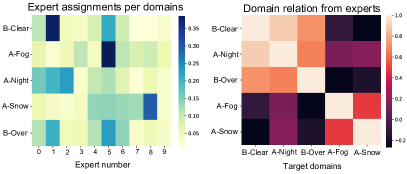
Figure 4: Expert Analysis. Left: We visualize the frequency of ten expert selections for each domain during CTTA. Our frequency map shows co-selected and isolated experts in different domains. Right: We interpret the similarity between target domains by visualizing the assignment weights from each domain-adaptive router.

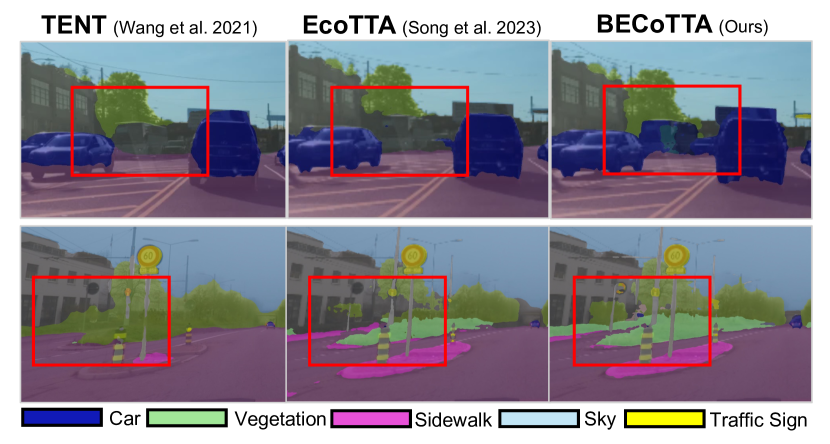
Figure 5: Pseudo label Visualization. Our BECoTTA generates more fine-grained and accurate labels than baselines.

Table 5: Ablation study for each element of the proposed BECoTTA. We measure the average IoU among 10 rounds.

DD	MoDE	$\Theta(D;A)$	Average IoU
			51.14
✔			51.18
✔	✔		53.87
✔	✔	✔	54.27

Table 6: Ablation of the quality of WAD. Our WAD has versatility with diverse augmentation methods.

WAD Augmentation	Round 1
	B-Clear	A-Fog	A-Night	A-Snow	B-Over	Avg
BECoTTA (Ours) - M	43.8	68.8	34.9	57.9	49.2	50.9
+ Style-transfer	45.6	70.8	42.6	59.7	50.8	53.9
+ Transformation	45.3	70	43.2	59.5	50.7	53.7

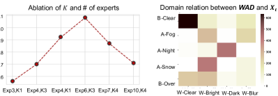
Figure 6: Detailed Analysis. We conduct the ablation study for the number of experts and $k$. Moreover, we analyze the relation between pre-defined WAD and target domains.

Ablation for each element. We observe the variation of the main components: Domain Discriminator (DD), MoDE, and domain-expert synergy loss $\Theta(D;A)$. As shown in Tab. 6, relying solely on DD results in only +0.04%p improvement compared with the source only. However, when incorporating the MoDE and $\Theta(D;A)$, there are +5.36%p and +6.12%p improvement respectively, comparing with the source model.

Quality of WAD. We adopt different augmentation methods to build realistic WAD. We utilize TSIT (Jiang et al., 2020) for style-transfer and PyTorch transformation (e.g., ColorJitter, RandomGrayscale), same as EcoTTA (Song et al., 2023). As shown in Tab. 6, we verify that the quality of WAD is a less important factor to have an effect on our domain-adaptive architecture. This demonstrates that our BECoTTA is implemented with various augmentations, showing its potential for expansion in diverse situations.

Effect of the number of $\bm{N}$ and $\bm{K}$. Our BECoTTA allows for the adjustment of the number of parameters and the complexity by varying $N$ (the whole number of experts) and $K$ (the number of selected experts). In Fig. 6 left, we illustrate these effects on the CDS-Hard scenario. From this, it is evident that the optimal results are obtained with $N$=6 and $k$=3. However, through numerous experiments, we find that regardless of the $N$ and $K$ chosen, our method consistently outperforms the existing baselines, demonstrating that our method is robust to hyperparameter settings.

Relation between WAD and $\bm{X_{t}}$. During the CTTA, we generate pseudo domain labels $d$ for each $X_{t}$ (target domains) through DD. These labels are used for initial domain-router assignment to facilitate domain-adaptive routing. Therefore, the relevance between the WAD and the target domain is crucial. In  Fig. 6 right, we represent the relationship between pre-defined WAD and $X_{t}$, and our DD faithfully reflects this connection.

5 Conclusion

We propose BECoTTA, an efficient yet powerful approach for CTTA, mainly consisting of Mixture-of-Domain Low-rank Experts (MoDE). Our MoDE has two key components: (i) domain-adaptive routing, and (ii) domain-expert synergy loss to maximize the dependency between each domain and expert. We show that our BECoTTA outperforms other SoTA continual TTA models and exhibits significant efficiency with fewer parameters and memory. Besides, ours shows strong potential for zero-shot domain generalization tasks. To facilitate the understanding of our proposed method, we extensively provide various analyses, including ablations of each component of BECoTTA and WAD strategies, and visualize the obtained pseudo labels and the relationships between domains and experts.

Broader Impact

In this work, we suggest BECoTTA and verify the superiority of performance and effectiveness. Due to its efficiency, our BECoTTA is highly effective when deployed on real-world embodied devices. This is particularly true in autonomous driving environments, where efficient adaptation is crucial. Moreover, it is freely applied to various real-world application branches, including health care and the medical field, which require continual adaptation. Therefore, we are confident that BECoTTA will have a significant impact on the practical application. We hope that our research focusing on efficiency contributes to the field of CTTA.

In this Appendix, we present the detailed material for the better understanding:

First, we provide additional information about CTTA baselines Sec. A and implementation details Sec. B. Moreover, additional experiment results in up to 10 rounds, including CDS-Easy, CDS-Hard, Continual Gradual Shifts (CGS) scenarios are provided at  Sec. C. We also provide various ablation studies with diverse combinations of our architectures. At the end, more detail about the data construction process is provided in  Sec. D.

Appendix A Baselines

In this section, we provide the details of the TTA baselines we use in our main paper.

CoTTA (Wang et al., 2022a) is a landmark work that proposed weight, augmentation averaged predictions, and stochastic restoration based on the mean-teacher framework. We utilize the official codes based on mmsegmentation that CoTTA author provided.

TENT (Wang et al., 2020) stands out as the pioneering approach to entropy minimization during testing, aiming to adapt to data shifts without the need for additional losses or data. We follow the above implementation from CoTTA authors.

SAR (Niu et al., 2023) point out a sharpness-aware entropy minimization that mitigates the impact of specific noisy test samples characterized by substantial gradients. As SAR has not been specifically validated in segmentation scenarios, we refer to their code base and reimplement it in the mmsegmentation framework.

EcoTTA (Song et al., 2023) propose memory-efficient architecture using meta networks. We believe there are similarities between our model and EcoTTA, particularly in emphasizing efficiency through the activation of small parts of the source model. To ensure a fair comparison, we align EcoTTA’s source model with our ViT-based Segformer. Behind each stage of Segformer, we insert their meta networks only four times in the source model ($K$=4).

Appendix B Experiment Details

B.1 Implementation Details

We provide the implementation details utilized in our experiments in Tabs. 8 and 7.

Table 7: Baseline method hyperparameters.

EcoTTA (Song et al., 2023)	$K$=4, $\lambda$=0.5, $H_{0}$=0.4
Ours	$\lambda_{d}$=0.1, $\lambda_{m}$=0.0005, $\kappa$=0.4

Table 8: Our method hyperparameters.

	Warm-up	TTA
Dataset	WAD	Target domains
Optimizer	AdamW	Adam
Optimizer momentum	$(\beta_{1},\beta_{2})=(0.9,0.999)$
Epoch	10	Online
Batch size	1
Learning rate	0.00006	0.00006/100
Label accessibility	Yes	No

B.2 The details of BECoTTA

The size of BECoTTA. Our BECoTTA has a flexible architecture design, which means we adjust the number of TTA parameters freely in various ways, depending on factors such as rank $r$, the insertion position of MoDE, and the number of experts $N$ in each MoDE. (All of the ‘parameters’ in our main paper mean the number of updated parameters in the TTA process.) For the main experiments, we adopt four experts for S, and only injected MoDE into the last block. Both M and L utilize six experts for MoDE, with the only difference being the rank.

Details of w/ & w/o WAD. To ensure a fair comparison, we conduct all experiments in w/ & w/o WAD settings. In the case w/o WAD, it is impossible to collect priors for domain candidates, therefore we adopt a single router $G$, similar to the conventional stochastic routing (Zuo et al., 2021). In settings w/ WAD, as described in the paper, we employ domain-adaptive routing and a domain-experts synergy loss. This approach maximizes the effectiveness of BECoTTA.

Appendix C Additional Quantitative Results

C.1 Results up to round 10

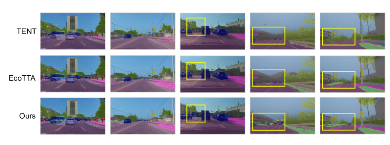
Figure 8: Pseudo labels from finished training up to round 10 in the CDS-Hard (imbalanced weather & area shifts) scenario. We visualize pseudo labels from BDD100k and ACDC datasets with other baselines. Our BECoTTA generates more fine-grained labels than other baselines.

Following the previous works, such as CoTTA (Wang et al., 2022a), we repeat ten rounds to simulate long-term continual domain shifts. Therefore, as shown in Tab. 9, Tab. 10, and Tab. 11, we provide the whole performance up to 10 rounds for each CDS-Easy, CDS-Hard, and Continual Gradual Shifts (CGS) scenarios. We also illustrate more qualitative results in  Fig. 8.

Table 9: Quantitative results of CDS-Easy (balanced weather shifts). We conduct experiments with Cityscapes-to-ACDC benchmarks which contain the weather shifts in the target domains. For a fair comparison, we report both w/o WAD and w/ WAD performance of our models.

Round		1				3				7				10
Method	Venue	Fog	Night	Rain	Snow	Fog	Night	Rain	Snow	Fog	Night	Rain	Snow	Fog	Night	Rain	Snow	Mean
Source only	NIPS’21	69.1	40.3	59.7	57.8	69.1	40.3	59.7	57.8	69.1	40.3	59.7	57.8	69.1	40.3	59.7	57.8	56.7
BN Stats Adapt (Nado et al., 2020)	-	62.3	38.0	54.6	53.0	62.3	38.0	54.6	53.0	62.3	38.0	54.6	53.0	62.3	38.0	54.6	53.0	52.0
Continual TENT (Wang et al., 2020)	ICLR’21	69.0	40.2	60.1	57.3	68.3	39.0	60.1	56.3	64.2	32.8	55.3	50.9	61.8	29.8	51.9	47.8	52.3
CoTTA (Wang et al., 2022a)	CVPR’22	70.9	41.2	62.4	59.7	70.9	41.0	62.7	59.7	70.9	41.0	62.8	59.7	70.8	41.0	62.8	59.7	58.6
SAR (Niu et al., 2023)	ICLR’23	69.0	40.2	60.1	57.3	69.1	40.3	60.0	57.8	69.1	40.2	60.3	57.9	69.1	40.1	60.5	57.9	56.8
EcoTTA (Song et al., 2023)	CVPR’23	68.5	35.8	62.1	57.4	68.1	35.3	62.3	57.3	67.2	34.2	62.0	56.9	66.4	33.2	61.3	56.3	55.2
BECoTTA (Ours)-S		71.3	41.1	62.4	59.8	71.4	41.1	62.4	59.8	71.3	41.1	62.4	59.8	71.3	41.2	62.3	59.8	58.6
+ WAD		72.0	45.4	63.7	60.0	71.7	45.4	63.6	60.1	71.8	45.4	63.7	60.1	71.7	45.3	63.6	60.0	60.2
BECoTTA (Ours)-M		72.3	42.0	63.5	60.1	72.3	41.9	63.6	60.2	72.3	41.9	63.6	60.3	72.3	41.9	63.5	60.2	59.4
+ WAD		71.8	48.0	66.3	62.0	71.8	47.7	66.3	61.9	71.8	47.8	66.4	61.9	71.8	47.9	66.3	62.6	62.0
BECoTTA (Ours)-L		71.5	42.6	63.2	59.1	71.5	42.5	63.2	59.1	71.5	42.5	63.2	59.1	71.6	42.5	63.1	59.1	59.1
+ WAD		72.7	49.5	66.3	63.1	72.5	49.7	66.2	63.1	72.3	49.5	66.2	63.1	72.1	49.2	66.2	63.2	63.0

Table 10: Results on CDS-Hard (imbalanced weather & area shifts). We devise a novel scenario encompassing imbalanced weather and area shifts. We present performance results for both w/o WAD and w/ WAD across the overall baselines. We report $S$, $M$, and $L$ versions for our BECoTTA based on the number of parameters.

Round			1						4						$\Delta$	Parameter
Init	Method	Init update	B-Clear	A-Fog	A-Night	A-Snow	B-Overcast	Mean	B-clear	A-Fog	A-Night	A-Snow	B-Overcast	Mean
	Source only	-	41.0	64.4	33.4	54.3	46.3	47.9	41.0	64.4	33.4	54.3	46.3	47.9	+0.0	-
	CoTTA (Wang et al., 2022a)	-	43.3	67.3	34.8	56.9	48.8	50.2	43.3	67.3	34.8	56.9	48.8	50.2	+0.0	54.72M
	TENT (Wang et al., 2020)	-	41.1	64.9	33.2	54.3	46.3	47.9	38.6	62.0	28.3	49.1	41.6	43.9	-4.0	0.02M
w/o WAD	SAR (Niu et al., 2023)	-	41.0	64.5	33.4	54.5	46.6	48.0	41.4	64.8	33.1	54.8	46.9	48.2	+0.2	0.02M
	EcoTTA (Song et al., 2023)	MetaNet	44.1	69.6	35.3	58.2	49.6	51.3	44.0	69.2	34.7	57.9	49.1	50.9	-0.4	3.46M
	BECoTTA (Ours)-S	MoDE	42.9	68.5	35.0	57.2	47.8	50.5	43.0	69.5	35.1	57.2	47.8	50.7	+0.1	0.09M
	BECoTTA (Ours)-M	MoDE	43.8	68.8	34.9	57.9	49.2	50.9	43.7	68.9	34.8	57.9	49.3	50.9	+0.0	0.63M
	BECoTTA (Ours)-L	MoDE	43.9	69.1	35.0	58.3	50.2	51.3	44.0	69.1	35.1	58.3	50.2	51.3	+0.0	3.16M
	Source only	Full	43.6	68.7	44.5	59.0	48.7	52.9	43.6	68.7	44.5	59.0	48.7	52.9	+0.0	-
	CoTTA (Wang et al., 2022a)	Full	46.4	70.6	45.7	61.2	51.3	55.0	46.1	70.5	45.6	61.1	51.2	54.9	-0.1	54.72M
	TENT (Wang et al., 2020)	Full	43.7	68.5	44.6	59.0	48.3	52.8	41.4	64.6	40.7	53.5	44.8	49.0	-3.8	0.02M
w/ WAD	SAR (Niu et al., 2023)	Full	43.6	68.6	44.5	59.1	48.7	52.9	43.7	69.1	36.4	56.8	48.3	50.8	-2.1	0.02M
	EcoTTA (Song et al., 2023)	MetaNet	44.6	70.2	41.6	58.0	49.9	52.9	43.7	69.1	36.4	56.8	48.3	50.8	-2.1	3.46M
	BECoTTA (Ours)-S	MoDE	44.1	69.5	40.1	56.8	49.1	51.9	44.0	69.4	40.2	56.9	49.2	51.8	+0.0	0.12M
	BECoTTA (Ours)-M	MoDE	45.6	70.8	42.6	59.6	50.8	53.9	45.6	70.8	42.6	59.5	50.8	53.9	+0.0	0.77M
	BECoTTA (Ours)-L	MoDE	45.7	71.4	43.7	59.6	50.5	54.2	45.7	71.3	43.7	59.6	50.6	54.2	+0.0	3.32M

Round			7						10						$\Delta$	Parameter
Init	Method	Init update	B-Clear	A-Fog	A-Night	A-Snow	B-Overcast	Mean	B-clear	A-Fog	A-Night	A-Snow	B-Overcast	Mean
	Source only	-	41.0	64.4	33.4	54.3	46.3	47.9	41.0	64.4	33.4	54.3	46.3	47.9	+0.0	-
	CoTTA (Wang et al., 2022a)	-	43.3	67.3	34.8	56.9	48.8	50.2	43.3	67.3	34.8	56.9	48.8	50.2	+0.0	54.72M
	TENT (Wang et al., 2020)	-	34.4	56.4	23.5	42.2	36.7	38.6	30.9	51.5	20.4	37.0	33.0	34.6	-13.3	0.02M
w/o WAD	SAR (Niu et al., 2023)	-	41.4	64.7	32.4	54.6	46.8	47.9	41.3	64.3	31.6	54.2	46.6	47.6	-0.4	0.02M
	EcoTTA (Song et al., 2023)	MetaNet	43.2	67.9	33.4	56.8	47.9	49.8	41.9	66.1	31.5	55.3	46.2	48.2	-3.1	3.46M
	BECoTTA (Ours)-S	MoDE	42.9	69.5	35.1	57.3	47.8	50.5	43.0	69.5	35.1	57.3	48.8	50.7	+0.1	0.09M
	BECoTTA (Ours)-M	MoDE	43.7	68.8	34.8	57.9	49.1	50.8	43.7	68.8	34.5	57.9	49.2	50.9	+0.0	0.63M
	BECoTTA (Ours)-L	MoDE	43.9	69.0	35.0	58.2	50.1	51.3	44.0	69.1	35.0	58.2	50.2	51.3	+0.0	3.16M
	Source only	Full	43.6	68.7	44.5	59.0	48.7	52.9	43.6	68.7	44.5	59.0	48.7	52.9	+0.0	-
	CoTTA (Wang et al., 2022a)	Full	46.1	70.5	45.6	61.1	51.2	54.9	46.1	70.5	45.6	61.1	51.2	54.9	-0.1	54.72M
	TENT (Wang et al., 2020)	Full	38.3	60.9	36.6	48.3	41.3	45.0	35.8	57.6	33.6	44.3	38.8	42.0	-10.8	0.02M
w/ WAD	SAR (Niu et al., 2023)	Full	43.6	67.9	43.1	58.6	48.5	52.3	43.4	67.4	42.2	58.1	47.6	51.9	-1.0	0.02M
	EcoTTA (Song et al., 2023)	MetaNet	42.3	67.3	32.1	55.8	46.7	48.8	41.1	65.6	27.0	53.2	45.3	46.4	-6.5	3.46M
	BECoTTA (Ours)-S	MoDE	44.0	69.4	40.2	56.8	49.2	51.9	44.0	69.4	40.1	56.9	49.1	51.9	+0.0	0.12M
	BECoTTA (Ours)-M	MoDE	45.6	70.6	42.6	59.6	50.8	53.8	45.6	70.7	42.5	59.5	50.8	53.9	+0.0	0.77M
	BECoTTA (Ours)-L	MoDE	45.6	71.3	43.7	59.5	50.5	54.2	45.7	71.3	43.7	59.6	50.6	54.2	+0.0	3.32M

Table 11: Quantitative results of Continual Gradual Shifts (CGS) scenarios. We present the results of up to ten rounds. Our CGS exhibits relatively higher performance across all models compared to the disjoint scenario, as neighboring domains are exposed within the scenario, unlike the conventional disjoint scenario.

Round		1				3				7				10
Method	Parameter	Task 1	Task 2	Task 3	Task 4	Task 1	Task 2	Task 3	Task 4	Task 1	Task 2	Task 3	Task 4	Task 1	Task 2	Task 3	Task 4	Mean
Source only	-	57.9	44.1	55.5	54.7	57.9	44.1	55.5	54.7	57.9	44.1	55.5	54.7	57.9	44.1	55.5	54.7	54.7
TENT (Wang et al., 2020)	0.02M	58.1	44.6	56.3	55.2	58.5	45.1	56.8	54.9	56.8	43.3	54.3	52.0	55.1	41.4	51.5	49.2	52.0
SAR (Niu et al., 2023)	0.02M	57.9	44.2	55.6	54.9	58.2	44.4	56.0	55.2	58.3	44.7	56.4	55.5	58.4	44.7	56.5	55.5	53.5
EcoTTA (Song et al., 2023)	3.46M	62.1	47.6	59.7	58.7	61.8	47.6	59.8	58.6	60.9	47.1	59.1	57.9	59.8	46.1	58.2	57.2	56.3
BECoTTA (Ours)-S	0.09M	61.8	46.9	57.6	56.9	61.8	46.9	57.6	56.9	61.6	49.8	57.7	57.0	61.7	49.7	57.5	57.1	55.8
+ WAD	0.12M	62.0	51.0	59.9	57.7	62.0	51.0	59.8	57.6	62.0	51.0	59.8	57.6	62.2	51.0	59.6	57.8	55.9
BECoTTA (Ours)-M	0.63M	60.4	46.2	58.2	57.4	60.5	46.2	58.2	57.4	60.5	46.2	58.2	57.5	60.5	46.2	58.2	57.4	55.5
+ WAD	0.77M	64.0	53.2	60.6	58.5	63.9	53.3	60.6	58.6	63.9	53.3	60.7	58.5	64.0	53.3	60.7	58.5	59.0
BECoTTA (Ours)-L	3.16M	62.5	47.7	59.3	59.0	62.5	47.7	59.3	59.0	62.4	47.8	59.2	58.8	62.5	47.7	59.1	58.8	57.1
+ WAD	3.31M	64.6	53.5	62.5	60.1	64.7	53.6	62.5	60.1	64.6	53.5	62.4	60.2	64.5	53.4	62.3	60.1	60.2

C.2 Additional Ablations

Table 12: Ablation study about warm-up loss weights. While doing this ablation, we set the hidden dimension as [8,8,16,32] and utilize six experts with $k$=3.

$\bm{\lambda_{s}}$	$\bm{\lambda_{m}}$	B-Clear	A-Fog	A-Night	A-Snow	B-Over	Avg
0.5	0.5	45.35	70.92	43.17	59.59	50.56	53.92
0.5	0.01	45.2	70.61	43.58	59.31	50.48	53.84
1	0.5	45.47	69.84	43.29	59.28	50.82	53.74
1	0.001	45.38	70.26	42.66	58.79	50.51	53.52
5	0.01	45.02	70.24	42.57	59.07	50.42	53.46

More about the loss weights. To assess the impact of warm-up loss weight $\lambda_{s}$ and $\lambda_{m}$, we conduct an ablation study in which $\lambda_{s}$ is the segmentation loss weight and $\lambda_{m}$ is the mutual loss weight in  Tab. 12. We fix the domain discriminator loss weight $\lambda_{d}$ while doing ablations. To precisely measure the effects, we evaluate the zero-shot performance for each domain, excluding the TTA process. The results indicate that as the weight of the mutual loss decreases, the performance of night scenes increases as it relatively diminishes consideration for mutual information. Furthermore, similar trends in performance are observed for adjusting the loss weight of similar images, such as {BDD-Clear, BDD-Overcast} and {ACDC-Fog, ACDC-Snow}.

More about the routing policy. We also conduct ablation studies on the routing policy for selecting experts within the MoDE layer. We measure the impact of the routing policy in the CDS-Hard scenario under the w/ WAD setting, where [2, 4, 10, 16] hidden dimensions and six experts with $k$=3. The multi-task performance refers to using a fixed assignment per domain, and stochastic routing (Zuo et al., 2021; Wang et al., 2022b) involves random-wise selection. According to  Tab. 13, our chosen top-k routing demonstrates the best performance. This is because the domain-specific router allows for routing that takes input-wise information into consideration.

Table 13: Ablation study for each routing policy. We conduct routing policy ablation using hidden dimension [2,4,10,16] with six experts.

	B-Clear	A-Fog	A-Night	A-Snow	B-Overcast	Avg
Multi-task	44.56	68.99	37.66	58.59	50.14	52.00
Stochastic	45.40	69.74	42.85	58.81	50.65	53.50
Top-K(Ours)	45.54	70.77	42.62	59.66	50.76	53.87

More about hidden dimension and the number of experts. We include results considering higher hidden dimensions and the number of experts in  Tab. 15, along with the consumption of parameters and memory. The hidden dimension refers to the rank $r$ for each encoder stage block for Segformer (Xie et al., 2021). For instance, [2,4,10,16] means each $r$=2,4,10,16 used at the MoDE layer for four stages Segformer (Xie et al., 2021). [0,0,0,16] denotes that the MoDE layer is used only in the last stage of the encoder. In particular, we predominantly opt for relatively low hidden dimensions and fewer experts, considering the trade-off with efficiency, even though setting a higher hidden dimension generally ensures better performance with more parameters.

C.3 Metrics for Continual Learning

Both CTTA and continual learning share the common objective of preventing forgetting to retain information encountered in the online stream. Therefore, we adopt the continual learning metrics (AvgIoU, BWT) for evaluating the forgetting phenomenon as represented in  Tab. 14.

AvgIoU denotes the overall performance while doing the learning process, and BWT evaluates the average influence of the current $N$th round on all of the previous tasks. These two metrics at the $k$th round are commonly defined as below. We measure the AvgIoU and BWT in the CTTA process after each round is finished.

$$AvgIoU_{k}=\frac{1}{\mathcal{D}}\sum_{j=1}^{\mathcal{D}}a_{kj}$$ (9)

$$BWT_{k}=\frac{1}{\mathcal{D}}\sum_{j=1}^{\mathcal{D}}a_{kj}-\tilde{a_{j}}$$ (10)

where $\mathcal{D}$ is the number of domains in each round, $a_{kj}$ denotes IoU evaluated by the model trained $k$ round for the $j$th domain, and $\tilde{a_{j}}$ represents IoU evaluated in the $j$th domain by the model trained up to the $j$th domain within the $k$ rounds.

Table 14: Quantitative results of AvgIoU and BWT. We evaluate AvgIoU and BWT among 3 rounds in the CDS-Hard scenario.

	Round 1		Round 2		Round 3		Avg
	AvgIoU	BWT	AvgIoU	BWT	AvgIoU	BWT	AvgIoU	BWT
TENT (Wang et al., 2020)	47.87	-0.15	46.63	-0.73	44.94	-0.97	46.48	-0.62
SAR (Niu et al., 2023)	48.11	0.08	48.19	0.04	48.23	0.01	48.18	0.04
BECoTTA (Ours) - M	51.29	0.15	51.33	0.17	51.33	0.16	51.32	0.16
+ WAD	54.32	0.26	54.30	0.30	54.30	0.31	54.31	0.29

In the case of TENT (Wang et al., 2020), both AvgIoU and BWT show a gradual decline as the round continues because of the severe effects of forgetting. However, our method addresses this forgetting effectively and shows the highest AvgIoU and BWT, especially when the effectiveness of domain-wise learning is maximized in w/WAD settings. In particular, the BWT improves as the round progresses, so it is interpreted that current learning has a positive effect on the past domains as learning continues.

Appendix D Dataset Construction

D.1 Scenario Construction Process

CDS-Easy scenario. As we mention in the main paper, we adopt the weather shift scenario in CTTA from CoTTA (Wang et al., 2022a) for a fair comparison. We set the target domain using the training set of the ACDC dataset, so the dataset for each domain consists of 400 unlabeled images, and their training order is as follows: $\{\textit{Fog}\rightarrow\textit{Night}\rightarrow\textit{Rain}\rightarrow\textit{Snow}\}$.

CDS-Hard scenario. To incorporate domain shift based on geographical factors and weather shifts from the Cityscapes-ACDC setting, we add clear and overcast datasets from BDD-100k as mentioned in the paper. We parse the official annotation json file to split the BDD-100k train dataset by weather conditions. For future reproducibility, we will publicly share the file list of our scenario. Consequently, we obtain a scenario sequence of $\{\textit{BDD-Clear}\rightarrow\textit{ACDC-Fog}\rightarrow\textit{ACDC-Night}\rightarrow\textit{ACDC-Snow}\rightarrow\textit{BDD-Overcast}\}$. Each of them consists of 500 unlabeled images. (We additionally add the ACDC 100 validation dataset together.)

D.2 Weather Augmented Dataset (WAD)

Generating process. We utilize the pre-trained style transformer TSIT (Jiang et al., 2020) to generate candidate domains using the Cityscapes (Cordts et al., 2016). For the candidate domains, we set dark, bright, and foggy styles to represent real-world weather practically as illustrated in  Fig. 7. We also apply the simple PyTorch augmentation to recreate them. Note that this process does not involve any training steps and resembles a one-time operation when setting the source domain. During the warm-up process, it enables the initialization from pre-defined domains by updating only the domain-wise routers and experts of the MoDE layer. Moreover, we have the flexibility to freely expand these candidate domains to others.

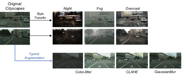
Figure 7: The example of generating WAD with different augmentation. We apply pre-trained style transfer and PyTorch augmentation for generating candidate domains for WAD.

Table 15: Further ablation study for the number of experts $N$, $K$, and hidden dimensions. We report sufficient ablation studies about the $N$, $K$, and hidden dimensions in the MoDE layer. All experiments are conducted in w/ WAD setting. ’Last’ denotes the MoDE layer located in the last stage of the encoder, whereas ’All’ denotes those located in every four stages of the encoder.

					Round 1
Parameters	Memory	Mode	Expert, K	Hidden dim	B-Clear	A-Fog	A-Night	A-Snow	B-Over	Avg
59,922	227.27MB		exp3 k1	[0, 0, 0, 2]	44.10	69.46	39.13	57.24	49.13	51.81
129,096	227.80MB		exp4 k1	[0, 0, 0, 6]	44.06	69.4	40.10	56.84	49.17	51.91
378,144	229.71MB		exp6 k3	[0, 0, 0, 16]	44.31	69.15	40.10	57.52	49.64	52.14
1,208,448	236.46MB		exp6 k3	[0, 0, 0, 64]	44.12	69.19	40.21	57.19	49.51	52.04
4,212,480	258.97MB		exp20 k10	[0, 0, 0, 64]	44.21	69.10	40.20	57.30	49.50	52.06
4,074,240	242.89MB	Last	exp10 k4	[0, 0, 0, 128]	43.91	68.48	39.31	56.52	49.28	51.50
779,916	231.36MB		exp6 k3	[2, 4, 10, 16]	45.45	70.77	42.62	59.66	50.76	53.85
956,976	232.71MB		exp6 k3	[8, 8, 16, 16]	45.54	70.40	42.76	59.50	50.90	53.82
1,252,176	234.96MB		exp6 k3	[8, 8, 16, 32]	45.21	70.53	43.26	59.32	50.69	53.80
1,299,860	236.92MB		exp10 k4	[2, 4, 10, 16]	45.47	69.56	43.04	58.88	50.54	53.50
2,599,720	247.03MB	All	exp20 k10	[2, 4, 10, 16]	45.33	70.17	43.13	59.48	51.04	53.83
3,469,312	251.21MB	EcoTTA + ViT (w/WAD)			44.64	70.21	41.68	58.02	49.94	52.9
4,554,528	261.60MB		exp3 k1	[32, 64, 160, 256]	45.28	70.22	43.14	58.74	50.42	53.56
6,072,704	273.20MB		exp4 k3	[32, 64, 160, 256]	45.16	70.41	42.91	59.65	50.39	53.70
9,109,056	296.39MB		exp6 k3	[32, 64, 160, 256]	45.45	70.61	44.32	59.40	50.61	54.08
15,181,760	342.77MB	All	exp10 k4	[32, 64, 160, 256]	46.17	71.3	43.47	60.63	51.18	54.55
477,805,276	533.81MB	Scratch CoTTA (w/WAD)			46.42	70.64	45.7	61.2	51.32	55.06

References

- Adachi et al. (2022) Adachi, K., Yamaguchi, S., and Kumagai, A. Covariance-aware feature alignment with pre-computed source statistics for test-time adaptation. arXiv preprint arXiv:2204.13263, 2022.
- Aljundi et al. (2019) Aljundi, R., Lin, M., Goujaud, B., and Bengio, Y. Gradient based sample selection for online continual learning. Advances in neural information processing systems, 32, 2019.
- Bang et al. (2021) Bang, J., Kim, H., Yoo, Y., Ha, J.-W., and Choi, J. Rainbow memory: Continual learning with a memory of diverse samples. In Proceedings of the IEEE/CVF conference on computer vision and pattern recognition, pp. 8218–8227, 2021.
- Bang et al. (2022) Bang, J., Koh, H., Park, S., Song, H., Ha, J.-W., and Choi, J. Online continual learning on a contaminated data stream with blurry task boundaries. In Proceedings of the IEEE/CVF Conference on Computer Vision and Pattern Recognition, pp. 9275–9284, 2022.
- Buslaev et al. (2020) Buslaev, A., Iglovikov, V. I., Khvedchenya, E., Parinov, A., Druzhinin, M., and Kalinin, A. A. Albumentations: Fast and flexible image augmentations. Information, 11(2), 2020. ISSN 2078-2489. doi: 10.3390/info11020125. URL https://www.mdpi.com/2078-2489/11/2/125.
- Choi et al. (2021) Choi, S., Jung, S., Yun, H., Kim, J. T., Kim, S., and Choo, J. Robustnet: Improving domain generalization in urban-scene segmentation via instance selective whitening. In Proceedings of the IEEE/CVF Conference on Computer Vision and Pattern Recognition, pp. 11580–11590, 2021.
- Choi et al. (2022a) Choi, S., Yang, S., Choi, S., and Yun, S. Improving test-time adaptation via shift-agnostic weight regularization and nearest source prototypes. In European Conference on Computer Vision, pp. 440–458. Springer, 2022a.
- Choi et al. (2022b) Choi, S., Yang, S., Choi, S., and Yun, S. Improving test-time adaptation via shift-agnostic weight regularization and nearest source prototypes. In European Conference on Computer Vision, pp. 440–458. Springer, 2022b.
- Cordts et al. (2016) Cordts, M., Omran, M., Ramos, S., Rehfeld, T., Enzweiler, M., Benenson, R., Franke, U., Roth, S., and Schiele, B. The cityscapes dataset for semantic urban scene understanding. In Proceedings of the IEEE conference on computer vision and pattern recognition, pp. 3213–3223, 2016.
- Fedus et al. (2022) Fedus, W., Zoph, B., and Shazeer, N. Switch transformers: Scaling to trillion parameter models with simple and efficient sparsity. The Journal of Machine Learning Research, 23(1):5232–5270, 2022.
- Gan et al. (2023) Gan, Y., Bai, Y., Lou, Y., Ma, X., Zhang, R., Shi, N., and Luo, L. Decorate the newcomers: Visual domain prompt for continual test time adaptation. In Proceedings of the AAAI Conference on Artificial Intelligence, volume 37, pp. 7595–7603, 2023.
- Gao et al. (2022a) Gao, J., Zhang, J., Liu, X., Darrell, T., Shelhamer, E., and Wang, D. Back to the source: Diffusion-driven test-time adaptation. arXiv preprint arXiv:2207.03442, 2022a.
- Gao et al. (2022b) Gao, Y., Shi, X., Zhu, Y., Wang, H., Tang, Z., Zhou, X., Li, M., and Metaxas, D. N. Visual prompt tuning for test-time domain adaptation. arXiv preprint arXiv:2210.04831, 2022b.
- Jiang et al. (2020) Jiang, L., Zhang, C., Huang, M., Liu, C., Shi, J., and Loy, C. C. Tsit: A simple and versatile framework for image-to-image translation. In Computer Vision–ECCV 2020: 16th European Conference, Glasgow, UK, August 23–28, 2020, Proceedings, Part III 16, pp. 206–222. Springer, 2020.
- Jung et al. (2023) Jung, S., Lee, J., Kim, N., Shaban, A., Boots, B., and Choo, J. Cafa: Class-aware feature alignment for test-time adaptation. In Proceedings of the IEEE/CVF International Conference on Computer Vision, pp. 19060–19071, 2023.
- Koh et al. (2021) Koh, H., Kim, D., Ha, J.-W., and Choi, J. Online continual learning on class incremental blurry task configuration with anytime inference. arXiv preprint arXiv:2110.10031, 2021.
- Lee et al. (2023a) Lee, J., Das, D., Choo, J., and Choi, S. Towards open-set test-time adaptation utilizing the wisdom of crowds in entropy minimization. In Proceedings of the IEEE/CVF International Conference on Computer Vision, pp. 16380–16389, 2023a.
- Lee et al. (2023b) Lee, T., Tremblay, J., Blukis, V., Wen, B., Lee, B.-U., Shin, I., Birchfield, S., Kweon, I. S., and Yoon, K.-J. Tta-cope: Test-time adaptation for category-level object pose estimation. In Proceedings of the IEEE/CVF Conference on Computer Vision and Pattern Recognition, pp. 21285–21295, 2023b.
- Lim et al. (2023) Lim, H., Kim, B., Choo, J., and Choi, S. Ttn: A domain-shift aware batch normalization in test-time adaptation. arXiv preprint arXiv:2302.05155, 2023.
- Liu et al. (2021) Liu, Y., Kothari, P., Van Delft, B., Bellot-Gurlet, B., Mordan, T., and Alahi, A. Ttt++: When does self-supervised test-time training fail or thrive? Advances in Neural Information Processing Systems, 34:21808–21820, 2021.
- Nado et al. (2020) Nado, Z., Padhy, S., Sculley, D., D’Amour, A., Lakshminarayanan, B., and Snoek, J. Evaluating prediction-time batch normalization for robustness under covariate shift. arXiv preprint arXiv:2006.10963, 2020.
- Neuhold et al. (2017) Neuhold, G., Ollmann, T., Rota Bulo, S., and Kontschieder, P. The mapillary vistas dataset for semantic understanding of street scenes. In Proceedings of the IEEE international conference on computer vision, pp. 4990–4999, 2017.
- Niu et al. (2022) Niu, S., Wu, J., Zhang, Y., Chen, Y., Zheng, S., Zhao, P., and Tan, M. Efficient test-time model adaptation without forgetting. In International conference on machine learning, pp. 16888–16905. PMLR, 2022.
- Niu et al. (2023) Niu, S., Wu, J., Zhang, Y., Wen, Z., Chen, Y., Zhao, P., and Tan, M. Towards stable test-time adaptation in dynamic wild world. arXiv preprint arXiv:2302.12400, 2023.
- Richter et al. (2016) Richter, S. R., Vineet, V., Roth, S., and Koltun, V. Playing for data: Ground truth from computer games. In Leibe, B., Matas, J., Sebe, N., and Welling, M. (eds.), European Conference on Computer Vision (ECCV), volume 9906 of LNCS, pp. 102–118. Springer International Publishing, 2016.
- Ros et al. (2016) Ros, G., Sellart, L., Materzynska, J., Vazquez, D., and Lopez, A. M. The synthia dataset: A large collection of synthetic images for semantic segmentation of urban scenes. In Proceedings of the IEEE conference on computer vision and pattern recognition, pp. 3234–3243, 2016.
- Sakaridis et al. (2021) Sakaridis, C., Dai, D., and Van Gool, L. Acdc: The adverse conditions dataset with correspondences for semantic driving scene understanding. In Proceedings of the IEEE/CVF International Conference on Computer Vision, pp. 10765–10775, 2021.
- Shazeer et al. (2017) Shazeer, N., Mirhoseini, A., Maziarz, K., Davis, A., Le, Q., Hinton, G., and Dean, J. Outrageously large neural networks: The sparsely-gated mixture-of-experts layer. arXiv preprint arXiv:1701.06538, 2017.
- Song et al. (2023) Song, J., Lee, J., Kweon, I. S., and Choi, S. Ecotta: Memory-efficient continual test-time adaptation via self-distilled regularization. In Proceedings of the IEEE/CVF Conference on Computer Vision and Pattern Recognition, pp. 11920–11929, 2023.
- Wang et al. (2020) Wang, D., Shelhamer, E., Liu, S., Olshausen, B., and Darrell, T. Tent: Fully test-time adaptation by entropy minimization. arXiv preprint arXiv:2006.10726, 2020.
- Wang et al. (2022a) Wang, Q., Fink, O., Van Gool, L., and Dai, D. Continual test-time domain adaptation. In Proceedings of the IEEE/CVF Conference on Computer Vision and Pattern Recognition, pp. 7201–7211, 2022a.
- Wang et al. (2022b) Wang, Y., Agarwal, S., Mukherjee, S., Liu, X., Gao, J., Awadallah, A. H., and Gao, J. Adamix: Mixture-of-adaptations for parameter-efficient model tuning. arXiv preprint arXiv:2210.17451, 2022b.
- Xie et al. (2021) Xie, E., Wang, W., Yu, Z., Anandkumar, A., Alvarez, J. M., and Luo, P. Segformer: Simple and efficient design for semantic segmentation with transformers. Advances in Neural Information Processing Systems, 34:12077–12090, 2021.
- Yu et al. (2020) Yu, F., Chen, H., Wang, X., Xian, W., Chen, Y., Liu, F., Madhavan, V., and Darrell, T. Bdd100k: A diverse driving dataset for heterogeneous multitask learning. In Proceedings of the IEEE/CVF conference on computer vision and pattern recognition, pp. 2636–2645, 2020.
- Zhong et al. (2022) Zhong, T., Chi, Z., Gu, L., Wang, Y., Yu, Y., and Tang, J. Meta-dmoe: Adapting to domain shift by meta-distillation from mixture-of-experts. Advances in Neural Information Processing Systems, 35:22243–22257, 2022.
- Zuo et al. (2021) Zuo, S., Liu, X., Jiao, J., Kim, Y. J., Hassan, H., Zhang, R., Zhao, T., and Gao, J. Taming sparsely activated transformer with stochastic experts. arXiv preprint arXiv:2110.04260, 2021.