Thermodynamics and Optical Properties of Phantom AdS Black Holes in Massive Gravity

Abstract

Motivated by high interest in Lorentz invariant massive gravity models known as dRGT massive gravity, we present an exact phantom black hole solution in this theory of gravity and discuss the thermodynamic structure of the black hole in the canonical ensemble. Calculating the conserved and thermodynamic quantities, we check the validity of the first law of thermodynamics and the Smarr relation in the extended phase space. In addition, we investigate both the local and global stability of these black holes and show how massive parameters affect the regions of stability. We extend our study to investigate the optical features of the black holes such as the shadow geometrical shape, energy emission rate, and deflection angle. Also, we discuss how these optical quantities are affected by massive coefficients. Finally, we consider a massive scalar perturbation minimally coupled to the background geometry of the black hole and examine the quasinormal modes (QNMs) by employing the WKB approximation.

I Introduction

Modified theories of gravity can explain some phenomena both from the perspective of cosmology and from the perspective of the astrophysical field, which general relativity was unable to describe. For example, the observational evidence of the current acceleration of our universe, dark energy, and dark matter problems. In addition, they almost inevitably require a spin$-2$ particle at their foundation. To include these issues, massive gravity is a fascinating theory of gravity that may include all of them. In this theory, the graviton includes mass which can describe, for example, the recent accelerated expansion at large distances. Historically, Pauli and Fierz introduced a linear theory of massive gravity in 1939 FP , to include massive graviton. However, this linear theory of massive gravity suffers from a fundamental law because in the massless limit of the graviton, it does not satisfy the observational evidence of the solar system. In this regard, Vainshtein extended it to include a non-linear case for removing this problem Vainshtein . However, it was indicated the existence of the ghost in this non-linear theory becomes another problematic factor which is known as Boulware and Deser (BD) ghost BD . The new massive gravity in three-dimensional spacetime is one of these attempts to remove BD-ghost in massive gravity Bergshoe2009 . Another commendable effort to remove this ghost is by introducing a reference metric which is known as dRGT massive gravity dRGT1 ; dRGT2 . In addition, this theory of massive gravity removes BD-ghost in arbitrary dimensional of spacetime Do104003 ; Do044022 . On the other hand, the black hole solutions may provide important tests of both the theoretical and phenomenological viability of dRGT massive gravity. In this regard, the black hole solutions in dRGT massive gravity are obtained extensively in the literature BHmass1 ; BHmass2 ; BHmass3 ; BHmass4 ; BHmass5 ; BHmass6 ; BHmass7 ; BHmass8 ; BHmass9 ; BHmass10 ; BHmass11 ; BHmass12 ; BHmass13 ; BHmass14 ; BHmass15 . The presence of additional terms in the black hole solutions can justify dark matter and dark energy in massive gravity. It was indicated that the massive graviton could play the role of the cosmological constant in cosmic distances Comelli2012 ; Langlois2012 ; Kobayashi2012 ; Felice2013 . In addition, the end state of Hawking evaporation led to a black hole remnant, which could help to ameliorate the information paradox BHmass14 . Also, in Ref. Hinterbichler2012 multi-gravity theory has been introduced to solve the BD-ghost in multi-dimensional spacetime for interacting spin-2 fields by applying the vielbein formulation. In another fascinating effort, it was indicated that by using a dynamic reference metric (instead of a static reference metric) the BD-ghost could be neglected in a non-linear bimetric theory for a massless spin-2 field Hassan2012 . Vegh introduced another branch of dRGT massive gravity by applying holographic principles and a singular reference metric Vegh . This theory was a ghost-free theory of massive gravity. By considering this theory of massive gravity, many works were done. For example, black hole solutions and their thermodynamic properties are investigated in Refs. VBHmass1 ; VBHmass2 ; VBHmass3 ; VBHmass4 ; VBHmass5 ; VBHmass6 ; Maetal2020 ; VBHmass7 ; VBHmass8 ; VBHmass9 . It was shown that there is a correspondence between black hole solutions of conformal and this theory of massive gravity Panah2019 . From an astrophysical point of view, the effect of massive graviton on the structure of neutron stars, white dwarfs, and dark energy stars has been studied in Refs. NeutronStar ; Whitedwarf ; DarkEnergyStar . The results indicated that the maximum mass of these compact objects could be more than three times of solar mass. In addition, by considering Vegh’s massive theory of gravity, the mass of the graviton could generate a range of new phase transitions for topological black holes Hendi2017 . Therefore, these issues motivated us to consider this theory of massive gravity.

In physics in general, we have some systems that present a peculiar characteristic, the energy density of the system is negative. We can cite some examples here Visser : a) the so-called usual Casimir effect, the case between two neutral plates, and the topological case; b) the case of the squeezed vacuum; c) the case of the Hartle-Hawking vacuum; and d) the case of a phantom field responsible for the accelerated expansion of the universe Caldwell . In gravitation, we also have similar cases. An example that draws our attention, is that of the quasi-charged bridge, built ad hoc by Einstein and Rosen in 1935 Einstein . This example introduces a charge of the system that appears with a sign opposite to that of the Reissner-Nordström solution, $q^{2}\rightarrow-q^{2}$. Thus, we have, in the action of the system, the first introduction of a spin-1 phantom field, with negative energy density. We also have the possibility of zero spin phantom fields, such as the anti-Fisher solution Bronnikov . The most general solutions of coupling scalar and Maxwell phantom fields are called Einstein-anti-Maxwell-anti-Dilaton Gerard . We have solutions with the cosmological constant Jardim2012 and regular Fabris . We have generalizations for phantom fields, using the Sigma model method, phantom solutions with rotation Gerard2 . Furthermore, we have the studies of the light path Azreg ; gravitational collapse Na ; gravitational lenses Gy ; global monopole Chen ; quasi-black holes Bronnikov2 ; dyon black holes Abishev ; wormholes Huang ; spherical accretion Azreg2 ; topological black holes in $f(R)$ Rodrigues ; and finally black bounces Silva .

Thermodynamic aspects of black holes have been among the most interesting subjects for many years. The studies on the black hole as a thermodynamic system date back to the work of Hawking and Bekenstein Bekenstein:1974 who demonstrated that geometrical quantities such as surface gravity and horizon area correspond to the thermodynamic quantities such as temperature and entropy. The analogy between the geometrical properties of the black holes and thermodynamic variables provides deep insight into understanding the relations between the physical properties of gravity and classical thermodynamics. Among the thermodynamical properties of black holes, phase transition and thermal stability have been widely studied in the literature Davies:197 ; Hawking:1983 ; Chamblin:1999 . Thermodynamic phase transition is one of the most interesting phenomena in black hole physics, which can provide insight into the underlying structure of spacetime geometry. Phase transition also plays an important role in elementary particle Kleinert:085001 , condensed matter Greer:1947 , usual thermodynamics Callen:1985 , cosmology Layzer:1991 , black holes Zou:2017 , and other branches of physics. In recent years, considerable attention has arisen to investigate the thermodynamic phase transition of black holes in anti-de-Sitter (AdS) spacetime. This is mainly motivated by AdS/CFT duality, which states that there exists a correspondence between gravity in an $(n+1)-$dimensional AdS spacetime and the conformal field theory living on the boundary of its n-dimensional spacetime Witten:1998 . Besides, studying the thermodynamic phase transition of black holes in such a spacetime provides a deep insight to understand the quantum nature of gravity, which is one of the most important theoretical subjects in physical communities. A significant interest has arisen to study the phase transition of AdS black holes in an extended phase space in which the cosmological constant can be regarded as a variable Kubiznak:1207 . In this viewpoint, the cosmological constant is identified as thermodynamic pressure, and the mass of the black hole is interpreted as the enthalpy Kastor:195011 . The study on phase transition in this phase space has disclosed some interesting phenomena, such as Van der Waals liquid-vapor phase transition Kubiznak:1207 ; Hendi2013 ; Cai2013 ; Xu2015 ; Singh2020 ; EslamPanah2020 , zeroth-order phase transition Doneva2010 , reentrant phase transition Kubiznak:1211 , triple critical point Wei:044057 . There are several methods to study the phase transition of black holes. The first method is based on studying heat capacity. It was pointed out that divergencies of the heat capacity represent phase transition points. Another approach is based on studying the van der Waals-like behavior of black holes in the extended phase space. In general, stability criteria can be categorized into two classes; dynamical stability and thermodynamical one. Thermodynamic stability of the black hole is of great importance because the instability of black holes puts restrictions on the validation of the physical solutions. One approach to investigating thermodynamic stability is through calculating heat capacity in the canonical ensemble. The sign of heat capacity represents the stability/instability of the black holes. Systems with positive (negative) heat capacity are denoted to be in thermally stable (unstable) states. Studying dynamical stability can be done by analyzing quasinormal modes (QNMs). In the literature, we will investigate both cases associated with phantom solutions Rodrigues3 ; Rodrigues4 .

The breakthrough discovery of the reconstruction of the event-horizon-scale images of the supermassive black holes by the Event Horizon Telescope (EHT) project shed light on the physics of black holes and provided us better insight into understanding these mysterious celestial objects. The experimental results reported by EHT Akiyama:2019L1 not only directly prove the existence of black holes, but also allow us to directly observe the shadows of black holes. Shadow is the image formed by null geodesics in the strong gravity regime. The formation of a black hole shadow depends on the angular momentum of photons. For low values of the angular momentum ($L$), ingoing photons fall into the black hole and form a dark area for a distant observer, whereas, for larger values of $L$, they will be deflected by the gravitational potential of the black hole. An interesting phenomenon is related to the photons with critical angular momentum. In this case, the photons orbit the black hole due to their non-vanishing transverse velocity and surround the dark interior, which are, respectively, called the photon ring and the black hole shadow. The shape and size of the shadow are determined by the black hole parameters, i.e., mass, angular momentum, and electric charge Vries:1999123 , as well as spacetime properties Johannsen:446 ; Cunha:024039 and the position of the observer. The image of a black hole gives us important information concerning jets and matter dynamics around black holes, and can be a useful tool for comparing alternative theories of gravity with general relativity. Moreover, the black hole shadow can be used to extract information about the deviations in the spacetime geometry Pedro:5042 ; Wei:08030 ; Belhaj:215004 . These deviations might be due to some parameters from different alternative theories of gravity Khodadi:104050 ; Uniyal:101178 , or the astrophysical environment in which the black hole is immersed Afrin:101195 ; Konoplya:933 . The history of the theoretical analysis of black hole shadow began with the seminal paper of Synge Synge:131 , who calculated the angular radius of the shadow of Schwarzschild black hole and showed the boundary of the shadow is a perfect circle for a non-rotating black hole. Then, Bardeen et al. Bardeen:347 analyzed the shadow of the Kerr black hole and argued that the black hole’s angular momentum causes the deformation of its shadow. Studying shadows has been extended to black holes in the modified theory of gravity Amarilla:124045 ; Kumar:100881 , to black holes with higher or extra dimensions Papnoi:024073 ; Amir:39978 , and black holes surrounded by plasma Atamurotov:084005 .

Black holes are interacting with the matter and radiations in the surroundings. The gravitational waves are the response of black holes to these perturbations, which were recently detected by LIGO Scientific Collaboration and Virgo Collaboration LIGO:241102 . The issue of the perturbations of black holes was first considered by Regge and Wheeler, who explored the stability of Schwarzschild black holes Wheeler:1063 . Studying black hole perturbations has been applied not only in the framework of GR Kokkota:1219 ; Cardoso:163001 ; Horowitz:024027 , but also in alternative gravity theories Kim:990 ; Kim:763 . The signal of the gravitational waves is dominated by the fundamental mode of the so-called QNMs of the black holes. QNMs are characteristic frequencies that encode the information on how black holes relax after the perturbation. From an astrophysical point of view, QNMs play an increasingly essential role in contemporary gravitational waves astronomy LIGO:061102 ; LIGO:161101 , because they can be regarded as characteristic ”sound” of black holes Nollert:1999 which serves as the basis of black holes spectroscopy. QNMs provide us with valuable information about the properties of black holes, such as their mass, angular momentum, and the nature of surrounding spacetime. QNM frequencies not only are an important factor in determining the parameters of black holes but also play a significant role in determining their space-time stability under perturbation. Studying QNMs can deepen our insight into the structure and evolution of black holes, and their role in astrophysical phenomena. Empirical detection of QNMs would not only provide us an opportunity to test general relativity and the validity of the famous ”no-hair” theorem of black holes Krishnan:787 ; Cardoso:064030 ; Giesler:111102 but also allow us to constrain modified gravity theories Liu:124011 ; Franciolini:12702 ; Gonzalez:2021 and examine strong cosmic censorship conjecture Cardoso:2018 ; Hod:941 ; Hod:2018 . Given the significance of QNMs introduced above, it will therefore be interesting to study QNMs when a new black hole solution is obtained.

Recently, it has been suggested that the real part of QNMs in the eikonal limit can be connected to the shadow radius of a black hole. Cardoso et al. Cardoso;2009 showed that the real part of the QNMs corresponds to the angular velocity of the unstable null geodesic while the imaginary part of the QNMs is related to the Lyapunov exponent that determines the instability timescale of the orbits. Such a connection can, alternatively, provide a physical picture at the semi-classical level, where the gravitational waves can be understood as a phenomenon in which a massless particle propagates along an outmost and unstable orbit of null geodesics and spreads transversely out to infinity Guo;084057 . The significance of this issue is in general to reach the relationship between gravitational waves and shadows of black holes, the two amazing achievements in the new century. The study connecting the real part of the QNMs and the shadow radius has been explored for the static Jusufi;084055 ; Melgar;13596 and the rotating spacetime Jusufi;124063 and has been also applied to different black holes Lan;115539 ; Wei;115103 ; Singh2022sU ; Myrzakulov2023 .

This work aims to obtain, through the equations of motion, a phantom AdS black hole solution, coupled with dRGT massive gravity; to study the horizons of the causal structure, the singularity, the thermodynamic system, and the main optical properties of the solution.

The paper is divided as follows: in section II, we define the action of the theory and establish the equations of motion; in section III, we impose the symmetry of the metric and the material content, studying the possible horizons and singularities; in section IV, we study the thermodynamics of the system, establishing the first law, the local and global stability; in section V, we present the main optical properties of our solution; we study the QNMs in section VI; and we end by presenting the final considerations in section VII.

II Field Equations

The $d$-dimensional form of Lagrangian of dRGT massive gravity is given by dRGT1 ; dRGT2

$$\mathcal{L}_{massive}=m_{g}^{2}\sum_{i}^{d}c_{i}\mathcal{U}_{i}(g,f),$$ (1)

where $m_{g}$ is the graviton mass parameter, $c_{i}$’s are arbitrary massive couplings and $\mathcal{U}_{i}$’s are graviton’s self-interaction potentials constructed from the building blocks $\mathcal{K}_{\,\,\,\nu}^{\mu}=\delta_{\nu}^{\mu}-\sqrt{g^{\mu\sigma}f_{ab}\partial_{\sigma}\phi^{a}\partial_{\nu}\phi^{b}}$ (where $g_{\mu\nu}$ is the dynamical (physical) metric, and $f_{\mu\nu}$ is the auxiliary reference metric, needed to define the mass term for gravitons as well as $\phi^{a}$’s are scalar fields well-known as Stückelberg fields), which can be written as

$$\mathcal{U}_{i}=\sum_{y=1}^{i}\left(-1\right)^{y+1}\frac{\left(i-1\right)!}{\left(i-y\right)!}\mathcal{U}_{i-y}\left[\mathcal{K}^{y}\right],$$ (2)

where $\mathcal{U}_{i-y}=1$, when $i=y$. The square root in $\mathcal{K}$ means $\left(\mathcal{K}\right)_{\lambda}^{\mu}\left(\mathcal{K}\right)_{\nu}^{\lambda}=\mathcal{K}_{\nu}^{\mu}$ and the rectangular brackets denote traces, $[\mathcal{K}]=\mathcal{K}_{\mu}^{\mu}$. The explicit form of $\mathcal{U}_{i}$’s can be written as follows

$$\mathcal{U}_{1} = \left[\mathcal{K}\right],\;\;\;\;\;\mathcal{U}_{2}=\left[\mathcal{K}\right]^{2}-\left[\mathcal{K}^{2}\right],\;\;\;\;\;\mathcal{U}_{3}=\left[\mathcal{K}\right]^{3}-3\left[\mathcal{K}\right]\left[\mathcal{K}^{2}\right]+2\left[\mathcal{K}^{3}\right],$$ (3)

$$\mathcal{U}_{4}=\left[\mathcal{K}\right]^{4}-6\left[\mathcal{K}^{2}\right]\left[\mathcal{K}\right]^{2}+8\left[\mathcal{K}^{3}\right]\left[\mathcal{K}\right]+3\left[\mathcal{K}^{2}\right]^{2}-6\left[\mathcal{K}^{4}\right].$$

The action of dRGT massive gravity with phantom Maxwell field on the $4-$dimensional spacetime and in the presence of the cosmological constant can be written as

$$\mathcal{I}=\int\sqrt{-g}\left[\mathcal{R}-2\Lambda-2\eta F_{\mu\nu}F^{\mu\nu}-\mathcal{L}_{massive}\right]d^{4}x,$$ (4)

in which we used geometric units in this work. Also, $\mathcal{R}$ and $\Lambda$ are the scalar curvature and the cosmological constant, respectively. In addition, $F_{\mu\nu}=\partial_{\mu}A_{\nu}-\partial_{\nu}A_{\mu}$ is the Faraday tensor with $A_{\mu}$ as the gauge potential. It is notable that, the first term characterizes the Einstein-Hilbert action, and the second term is related to the cosmological constant, which can behave as dS ($\Lambda>0$) or AdS ($\Lambda<0$). The third term is the coupling with the Maxwell field when $\eta=1$, or a phantom field of spin$-1$, when $\eta=-1$. In other words, the constant $\eta$ indicates the nature of the electromagnetic field. Indeed, we obtain the classical Einstein-Maxwell theory when $\eta=1$, whereas for $\eta=-1$, the Maxwell field is phantom (this phantom is because the energy density of the field of spin$-1$ is negative (see Ref. Jardim2012 , for more details)). The last term in the above action is related to the Lagrangian of dRGT massive gravity (Eq. (1)).

Taking the action (4) into account and using the variational principle, we obtain the field equations corresponding to the gravitation and gauge fields as

$$G_{\mu\nu}-\Lambda g_{\mu\nu}-m_{g}^{2}\chi_{\mu\nu} = 2\eta\left(\frac{g_{\mu\nu}}{4}F_{\mu\nu}F^{\mu\nu}-F_{\mu\rho}F_{\nu}^{\rho}\right),$$ (5)

$$\partial_{\mu}\left(\sqrt{-g}F^{\mu\nu}\right) = 0,$$ (6)

where $\chi_{\mu\nu}$ is given by

$$\chi_{\mu\nu}=-\sum_{i=1}^{d-2}\frac{c_{i}}{2}\left[\mathcal{U}_{i}g_{\mu\nu}+\sum_{y=1}^{i}\left(-1\right)^{y}\frac{i!}{\left(i-y\right)!}\mathcal{U}_{i-y}\mathcal{K}_{\mu\nu}^{y}\right].$$

The field equations turn to general relativity’s field equations when the graviton mass is zero ($m_{g}=0$), i.e., $G_{\mu\nu}-\Lambda g_{\mu\nu}=2\eta\left(\frac{g_{\mu\nu}}{4}F_{\mu\nu}F^{\mu\nu}-F_{\mu\rho}F_{\nu}^{\rho}\right)$ Jardim2012 .

III Phantom black hole solutions

Since we are interested in static phantom charged black hole solutions in massive gravity, we consider the metric of $4$-dimensional spacetime with the following form

$$ds^{2}=\psi\left(r\right)dt^{2}-\frac{dr^{2}}{\psi(r)}-r^{2}\left(d\theta^{2}+\sin^{2}\theta d\varphi^{2}\right),$$ (7)

in which $\psi(r)$ is the metric function of our black holes. In addition, the conventions adopted here are with the description of the metric whose signature is $(+,-,-,-)$.

Our main motivation is to obtain exact phantom black holes in the context of massive gravity. In this regard, the appropriate ansatz for the reference metric is as VBHmass1 ; VBHmass2

$$f_{\mu\nu}=diag\left(0,0,-c^{2},-c^{2}\sin^{2}\theta\right).$$ (8)

Before deriving the exact solution for AdS phantom black holes, we would like to explain the importance of choosing such a reference metric. As we know, to construct the non-linear massive gravity, introducing an auxiliary non-dynamical reference metric is necessary. However, the reference metric breaks the diffeomorphism invariance (also known as general covariance or coordinate invariance) of general relativity. The breakdown of diffeomorphism invariance implies that the two helicities $\pm 2$ of the massless graviton would be joined by four degrees to give six degrees of freedom BD . The sixth degree of freedom corresponds to BD ghost. One way to solve this problem is introducing a degenerate reference metric as $f_{\mu\nu}=diag(0,0,1,1)$ which was first defined by Vegh Vegh . Such a choice of reference metric depends only on the spatial components; therefore, the diffeomorphism invariance (general reference) is preserved in the $t$ and $r$ coordinates but is broken in the spatial dimensions. One can also imagine a more general reference metric that does not respect diffeomorphism invariance in the $r-direction$. For instance, to preserve rotational invariance on the sphere and general time parametrization invariance, one can choose $f_{\mu\nu}=diag(0,1,c^{2},c^{2}sin^{2}\theta)$ as a natural ansatz. One can also consider a different generalization of $f_{\mu\nu}$, with $sin^{2}\theta f_{\theta\theta}=f_{\varphi\varphi}=F(r)$, and all other components to be zero Adams91 . This can lead to an ability to add arbitrary polynomial terms in $r$ to the emblackening factor. The massive gravity of this choice of reference metric has important applications in gauge/gravity duality. Massive gravities on AdS with a degenerate reference metric can be viewed as effective dual-field theories of different phases of condensed matter systems with broken translational symmetry such as solids, (perfect) fluids, and liquid crystals Alberte114 ; Alberte171 ; Alberte129 . In fact, AdS black holes in massive gravity with a singular (degenerate) reference metric are proving useful in building holographic models for normal conductors that are close to realistic ones, with finite direct-current (DC) conductivity Blake88 ; Alberte91 , the desired property for normal conductors that is absent in massless gravities. However, such an investigation is not the purpose of this paper.

It is notable that for $d-$dimensional spacetime, the reference metric is $f_{\mu\nu}=diag\left(0,0,c^{2}h_{ij}\right)$ VBHmass1 , in which $h_{ij}$ determines by $d-$dimensional dynamical metric (i.e. $ds^{2}=\psi\left(r\right)dt^{2}-\psi^{-1}(r)dr^{2}-r^{2}h_{ij}dx^{i}dx^{j}$, $i,j=1,2,3,...,n$). In this case, the explicit functional forms of $U_{i}$’s are given by VBHmass1

$$\mathcal{U}_{1} = \frac{\left(d-2\right)c}{r},$$

$$\mathcal{U}_{2} = \frac{\left(d-2\right)\left(d-3\right)c^{2}}{r^{2}},$$

$$\mathcal{U}_{3} = \frac{\left(d-2\right)\left(d-3\right)\left(d-4\right)c^{3}}{r^{3}},$$

$$\mathcal{U}_{4} = \frac{\left(d-2\right)\left(d-3\right)\left(d-4\right)\left(d-5\right)c^{4}}{r^{4}}.$$ (9)

Using the mentioned information and ansatz (8), one can extract the explicit functional forms of $\mathcal{U}_{i}$ ’s, Since we are interested in $4-$dimensional solutions (i.e., $d=4$), the only non-zero terms of $\mathcal{U}_{i}$ are $\mathcal{U}_{1}$ and $\mathcal{U}_{2}$ while the quartic terms all vanish. By taking this fact into account, one can find the following action governing our black holes of interest

$$\mathcal{U}_{1} = \frac{2c}{r},~{}~{}~{}\&~{}~{}~{}\mathcal{U}_{2}=\frac{2c^{2}}{r^{2}},$$

$$\mathcal{U}_{i} = 0,\text{ \ \ when \ \ }i>2$$ (10)

To have a radial electric field, we consider the following gauge potential

$$A_{\mu}=h(r)\delta_{\mu}^{t},$$ (11)

where by using the metric (7) with the Maxwell field equation (6), one can find the following differential equation

$$h^{\prime}(r)+rh^{\prime\prime}(r)=0,$$ (12)

in which the prime and double prime are representing the first and second derivatives with respect to $r$, respectively. It is a matter of calculation to solve Eq. (12), yielding

$$h(r)=-\frac{q}{r},$$ (13)

where $q$ is an integration constant related to the electric charge. It is worthwhile to mention that the corresponding electromagnetic field tensor is $F_{tr}=\frac{q}{r^{2}}$.

In order to obtain the metric function, $f(r)$, we use Eq. (7) with Eq. (5), and obtain the following differential equations

$$e_{tt} = e_{rr}=\Lambda r^{2}+\left(\psi^{\prime}(r)-C_{1}\right)r+\psi\left(r\right)-1-C_{2}+\frac{\eta q^{2}}{r^{2}},$$ (14)

$$e_{\theta\theta} = e_{\varphi\varphi}=\left(\psi^{\prime\prime}(r)+2\Lambda\right)r^{2}+\left(2\psi^{\prime}(r)-C_{1}\right)r-\frac{2\eta q^{2}}{r^{2}},$$ (15)

where $C_{1}=m_{g}^{2}cc_{1}$, and $C_{2}=m_{g}^{2}c^{2}c_{2}$. Also, $e_{tt}$, $e_{rr}$, $e_{\theta\theta}$ and $e_{\varphi\varphi}$ correspond to $tt$, $rr$, $\theta\theta$ and $\varphi\varphi$ components of Eq. (5), respectively. Considering the equations (14) and (15), we can obtain the metric function in the following form

$$\psi(r)=1-\frac{2m_{0}}{r}-\frac{\Lambda r^{2}}{3}+\frac{\eta q^{2}}{r^{2}}+\frac{C_{1}r}{2}+C_{2},$$ (16)

where $m_{0}$ is an integration constant related to the total mass of the black hole. It is worthwhile to mention that the resulting metric function (16) satisfies all the components of the field equation (5), simultaneously. Whereas the constant term $C_{2}$ appears due to the existence of massive gravity (which acts as a modified term to Einstein’s gravity) and it compares with $1$, so this term cannot be more than $1$ (i.e., $\left|C_{2}\right|<1$). In addition, in the absence of massive parameter ($C_{1}=C_{2}=0$), the metric function Eq. (16) reduces to

$$\psi(r)=1-\frac{2m_{0}}{r}-\frac{\Lambda r^{2}}{3}+\frac{\eta q^{2}}{r^{2}}.$$ (17)

Our next step is the examination of the geometrical structure of solutions. First, we should look for the existence of essential singularity(ies). The Ricci and Kretschmann scalars of the solutions are, respectively,

$$R = -4\Lambda+\frac{3C_{1}}{r}+\frac{2C_{2}}{r^{2}},$$ (18)

$$R_{\alpha\beta\gamma\delta}R^{\alpha\beta\gamma\delta} = \frac{8\Lambda^{2}}{3}-\frac{4C_{1}\Lambda}{r}+\frac{2C_{1}^{2}-\frac{8\Lambda C_{2}}{3}}{r^{2}}+\frac{4C_{1}C_{2}}{r^{3}}-\frac{16C_{2}m_{0}+4C_{1}\eta q^{2}}{r^{5}}$$ (19)

$$+\frac{48m_{0}^{2}+8C_{2}\eta q^{2}}{r^{6}}+\frac{4C_{2}^{2}}{r^{4}}-\frac{96m_{0}\eta q^{2}}{r^{7}}+\frac{56\eta^{2}q^{4}}{r^{8}}.$$

These relations confirm that there is an essential curvature singularity at $r=0$. For the limit of $r\longrightarrow\infty$, the Ricci and Kretschmann scalars yield the values $4\Lambda$ and $\frac{8\Lambda^{2}}{3}$, respectively, which show that for $\Lambda>0$ ($\Lambda<0$), the asymptotical behavior of the solution is (A)dS.

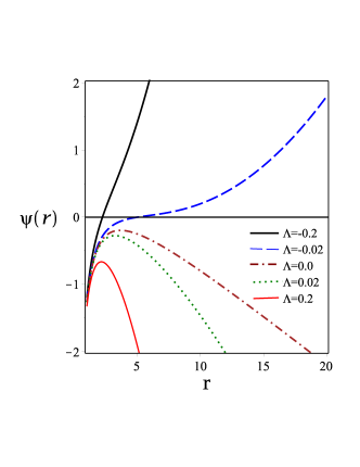
Figure 1: The metric function $\psi(r)$ versus $r$ for $q=0.1$, $m_{0}=1$, $C_{1}=-0.3$, $C_{2}=-0.1$, $\eta=-1$ and different values of the cosmological constant.

(a) $C_{2}=-0.069$ and $\Lambda=-0.02$

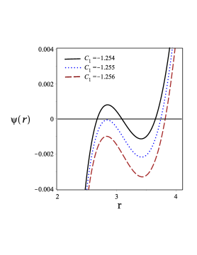
(b) $C_{2}=0.98$ and $\Lambda=-0.2$

Figure 2: The metric function $\psi(r)$ versus $r$ for different values of $C_{1}$ and $\eta=-1$.

In Ref. Panah2019 a correspondence between black hole solutions of conformal and massive theories of gravity is found which imposed some constraints on the parameters of massive gravity, which are;

Constraint (i): $C_{1}<0$ and $C_{2}<0$.

Constraint (ii): $C_{1}>0$ and $C_{2}<0$.

Also, these constraints are compatible from the astrophysical point of view for the study of neutron stars, white dwarfs, and dark energy stars NeutronStar ; Whitedwarf ; DarkEnergyStar . Applying Constraint (i), i.e., $C_{1}<0$ and $C_{2}<0$, and special negative values of $C_{1}$ and $C_{2}$, we plot the Figure. 1. Our results show that there is no root for $\Lambda>0$ and $\Lambda=0$. Indeed, for special negative values of parameters $C_{1}$ and $C_{2}$, phantom dS and flat black holes do not have any root, but phantom AdS black holes (i.e., $\Lambda<0$) have one root or an event horizon (see the continuous and dashed lines in Fig. 1).

Another interesting result is related to the existence of multi-horizons for phantom AdS black holes. In other words, by considering negative values for the cosmological constant and other parameters, we can find black holes with one root or an event horizon (see the dashed line in Fig. 2(a)); two roots, an inner root, and an event horizon (see the dotted line in Fig. 2(a)), and multi-horizons which include two inner roots and an event horizon (see the continuous line in Fig. 2(a)). In Fig. 2(b), we considered $\Lambda=-0.2$ and studied the existence of multi-horizons for the mentioned black holes. One can see that such behavior is observed for $C_{2}$ very close to 1, which is not acceptable according to what was already mentioned. Therefore, the existence of multi-horizons for phantom AdS black holes is only visible for very small values of $|\Lambda|$.

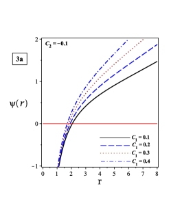
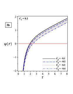
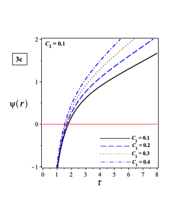
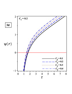
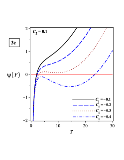
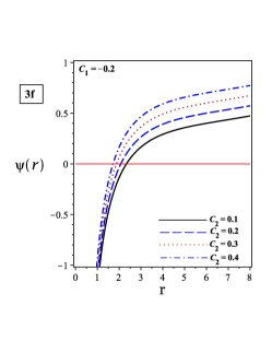
Figure 3: The metric function $\psi(r)$ versus $r$ for $q=0.5$, $m_{0}=1$, $\eta=-1$, and $\Lambda=-0.02$. Left panels for different values of $C_{1}$, and right panels for different values of $C_{2}$.

To evaluate the effects of massive parameters with different signatures and values, we plot six panels in Fig. 3. Our analysis indicates that:

i) By considering the negative value of $C_{2}$, the radii of phantom AdS black holes decrease by increasing the positive value of $C_{1}$ (see Fig. 3a).

ii) For the positive constant value of $C_{1}$, we encounter with large phantom AdS black holes when the negative value of $C_{2}$ increases (see Fig. 3b).

iii) The radii of phantom AdS black holes decrease when the positive value of $C_{1}$ increases, provided $C_{2}>0$ (see Fig. 3c).

iv) For $C_{1}>0$, by increasing the positive value of $C_{2}$, the radii of these black holes decreases (see Fig. 3d).

v) By increasing negative value of $C_{1}$, we encounter with large black holes when $C_{2}>0$ (see Fig. 3e).

vi) By considering the negative value of $C_{1}$, the radii of phantom AdS black holes decrease by increasing the positive value of $C_{2}$ (see Fig. 3f).

IV Thermodynamics

In this section, we first calculate the conserved and thermodynamic quantities of the phantom black hole solutions in massive gravity. We extend phase space to the extended phase space by considering the cosmological constant as a thermodynamic variable corresponding to pressure and check the first law of thermodynamics and the Smarr relation. After that, we investigate the local and global stability of these black holes by employing heat capacity, and Helmholtz free energy.

IV.1 Thermodynamic Quantities, First Law, and Smarr Relation

Here, we get the conserved and thermodynamic quantities of these black holes, which are necessary to study thermodynamic properties. For this purpose, we express the mass ($m_{0}$) in terms of the radius of the event horizon $(r_{e})$ and other quantities of these solutions such as, the charge $(q)$, the cosmological constant ($\Lambda$), and massive parameters ($C_{1}$, and $C_{2}$) in the following equation which is extracted by equating $g_{tt}=\psi(r)$ to zero

$$m_{0}=\frac{-\Lambda r_{e}^{3}}{6}+\frac{C_{1}r_{e}^{2}}{4}+\frac{\left(1+C_{2}\right)r_{e}}{2}+\frac{\eta q^{2}}{2r_{e}}.$$ (20)

In order to get the Hawking temperature, we obtain the superficial gravity for these black holes as

$$\kappa=\left.\frac{g_{tt}^{\prime}}{2\sqrt{-g_{tt}g_{rr}}}=\right|_{r=r_{e}}=\left.\frac{\psi^{\prime}(r)}{2}\right|_{r=r_{e}},$$ (21)

by substituting the mass (20) within the equation (21) and using the obtained metric function, one can calculate the superficial gravity which is given by

$$\kappa=\frac{-\Lambda r_{e}}{2}+\frac{C_{1}}{2}+\frac{1+C_{2}}{2r_{e}}-\frac{\eta q^{2}}{2r_{e}^{3}},$$ (22)

now, we can get the Hawking temperature in the following form

$$T=\frac{\kappa}{2\pi}=\frac{-\Lambda r_{e}}{4\pi}+\frac{C_{1}}{4\pi}+\frac{1+C_{2}}{4\pi r_{e}}-\frac{\eta q^{2}}{4\pi r_{e}^{3}}.$$ (23)

Another thermodynamic quantity is the electric charge. We can obtain it by using the Gauss law. So, the electric charge of the black hole per unit volume is given

$$Q=\frac{F_{tr}}{4\pi}\int_{0}^{2\pi}\int_{0}^{\pi}\sqrt{g}d\theta d\varphi=\frac{q}{4\pi},$$ (24)

in the above equation, $F_{tr}=\frac{q}{r^{2}}$, and for case $t=$ constant and $r=$constant, the determinant of metric tensor $g$ is given by $r^{4}\sin^{2}\theta$.

We find the electric potential ($U$) at the event horizon with respect to the reference ($r\rightarrow\infty$) by using the definition $U=-\int_{r_{e}}^{+\infty}F_{tr}dr$, where $F_{tr}=\partial_{t}A_{r}-\partial_{r}A_{t}$. This quantity is

$$U=\frac{q}{r_{e}}.$$ (25)

One can use the area law to extract the entropy of black holes, which leads to

$$S=\frac{\mathcal{A}}{4},$$ (26)

where $\mathcal{A}$ is the horizon area. The horizon area per unit volume is given by

$$\mathcal{A}=\left.\int_{0}^{2\pi}\int_{0}^{\pi}\sqrt{g_{\theta\theta}g_{\varphi\varphi}}\right|_{r=r_{e}}=\left.r^{2}\right|_{r=r_{e}}=r_{e}^{2},$$ (27)

by replacing the horizon area (27) within Eq. (26), we can get the entropy of phantom black holes per unit volume in massive gravity in the following form

$$S=\frac{r_{e}^{2}}{4}.$$ (28)

In the extended phase space, the cosmological constant acts as a thermodynamic variable corresponding to pressure

$$P=\frac{-\Lambda}{8\pi},$$ (29)

where this postulate leads to an interpretation of the black hole mass as enthalpy Kastor .

We obtain the total mass of these black holes per unit volume by using Ashtekar-Magnon-Das (AMD) approach AMDI ; AMDII which is extracted

$$M=\frac{m_{0}}{4\pi},$$ (30)

where substituting the mass (20) and $\Lambda=-8\pi P$ within the equation (30), we find

$$M=\frac{r_{e}^{3}P}{3}+\frac{C_{1}r_{e}^{2}}{16\pi}+\frac{\left(1+C_{2}\right)r_{e}}{8\pi}+\frac{\eta q^{2}}{8\pi r_{e}}.$$ (31)

It is straightforward to show that the conserved and thermodynamic quantities satisfy the first law of thermodynamics in extended phase space in the following form

$$dM=TdS+\eta UdQ+VdP+\mathcal{C}_{1}dC_{1}+\mathcal{C}_{2}dC_{2},$$ (32)

where the conjugate quantities associated with the intensive parameters $S,Q,P,C_{i}$’s are

$$T = \left(\frac{\partial M}{\partial S}\right)_{Q,P,C_{i}},$$

$$\eta U = \left(\frac{\partial M}{\partial Q}\right)_{S,P,C_{i}},$$

$$V = \left(\frac{\partial M}{\partial P}\right)_{S,Q,C_{i}}=\frac{r_{e}^{3}}{3},$$

$$\mathcal{C}_{1} = \left(\frac{\partial M}{\partial C_{1}}\right)_{S,Q,C_{2}}=\frac{r_{e}^{2}}{16\pi},$$

$$\mathcal{C}_{2} = \left(\frac{\partial M}{\partial C_{2}}\right)_{S,Q,C_{1}}=\frac{r_{e}}{8\pi},$$ (33)

where $T=\left(\frac{\partial M}{\partial S}\right)_{Q,P,C_{i}}$ and $\eta U=\left(\frac{\partial M}{\partial Q}\right)_{S,P,C_{i}}$ are in agreement with those of calculated in Eqs. (23) and (25), respectively, provided $\Lambda=-8\pi P$.

It is notable that an active astrophysical black hole is always surrounded by an accretion disk containing various types of baryonic matter, including electric charges. With our first law of thermodynamics, we can describe how energy is exchanged between the black hole and its surroundings. A striking feature of phantom solutions is the change in sign of the work term ($UQ$ in Eq. (32)), which indicates negative energy from electromagnetic action. When this type of energy is exchanged for work done or received by the black hole, the contribution will be symmetrical to that of a normal solution.

Despite this strong characteristic in ghost solutions, the thermodynamic system can present itself like all asymptotically AdS black hole solutions, i.e. the black hole can start by accreting matter and increasing its entropy, initially in an unstable small black hole phase (small event horizon area). As the black hole accretes more matter, it can move on to a new phase, called a large black hole (large area), where the thermodynamic system is stable. So even if the solution is phantom, but the black hole may be in a thermodynamically stable phase in nature.

The Smarr relation can be derived by a scaling (dimensional) argument as

$$M=2\left(TS-PV\right)+\eta UQ-\mathcal{C}_{1}C_{1},$$ (34)

where $C_{2}$ does not appear in the Smarr relation since it has scaling weight $0$ Hendi2017 . Indeed, the $C_{2}$ term in the metric function is a constant term in $4-$dimensional spacetime with no thermodynamical contribution, so we set $dC_{2}=0$.

IV.2 Local thermal stability in canonical ensemble

In the canonical ensemble context, the local stability of a thermodynamic system is determined by studying the heat capacity. Indeed, the discontinuities of this quantity mark the possible thermal phase transitions that the system can undergo. Also, the positivity of the heat capacity corresponds to thermal stability while the opposite indicates instability. Moreover, the roots of heat capacity may yield possible changes between stable/unstable states (or bound points). To get this information, we calculate the heat capacity of the solutions and investigate the local stability of the phantom black holes. We also study the effects of parameters of massive gravity on local stability areas.

To obtain the heat capacity, we first re-write the total mass of the black hole (31) in terms of the electrical charge (24), the entropy (28), pressure (29) and massive parameters as

$$M\left(S,Q,P,C_{i}\right)=\frac{\pi\eta Q^{2}}{\sqrt{S}}+\frac{\left(1+C_{2}\right)\sqrt{S}}{4\pi}+\frac{C_{1}S}{4\pi}+\frac{8PS^{3/2}}{3},$$ (35)

we re-write the temperature by using the equation (35)

$$T=\left(\frac{\partial M\left(S,Q,P,C_{i}\right)}{\partial S}\right)_{Q,P,C_{i}}=4P\sqrt{S}+\frac{C_{1}}{4\pi}+\frac{1+C_{2}}{8\pi\sqrt{S}}-\frac{\pi\eta Q^{2}}{2S^{3/2}}.$$ (36)

Now, we can obtain the heat capacity which is defined

$$C_{Q,P,C_{i}}=\frac{T}{\left(\frac{\partial T}{\partial S}\right)_{Q,P,C_{i}}}=\frac{\left(\frac{\partial M\left(S,Q,P,C_{i}\right)}{\partial S}\right)_{Q,P,C_{i}}}{\left(\frac{\partial^{2}M\left(S,Q,P,C_{i}\right)}{\partial S^{2}}\right)_{Q,P,C_{i}}},$$ (37)

by considering Eqs. (35) and (36), the heat capacity is given by

$$C_{Q,P,C_{i}}=\frac{2\left(32\pi PS^{2}+2C_{1}S^{3/2}\right)}{12\pi^{2}\eta Q^{2}-\left(1-32\pi PS+C_{2}\right)S}+\frac{\left(1+C_{2}\right)S-4\pi^{2}\eta Q^{2}}{6\pi^{2}\eta Q^{2}-\frac{\left(1-32\pi PS+C_{2}\right)S}{2}}.$$ (38)

By studying the heat capacity of the black hole, we can find two important points that are related to the physical limitation and phase transition critical points. Indeed, the root of heat capacity $\left(C_{Q,P,C_{i}}=0\text{, or }T=\left(\frac{\partial M\left(S,Q,P,C_{i}\right)}{\partial S}\right)_{Q,P,C_{i}}=0\right)$ is representing a border line between physical $\left(\left(\frac{\partial M\left(S,Q,P,C_{i}\right)}{\partial S}\right)_{Q,P,C_{i}}>0\right)$ and non-physical $\left(\left(\frac{\partial M\left(S,Q,P,C_{i}\right)}{\partial S}\right)_{Q,P,C_{i}}<0\right)$ black holes (which is known as the physical limitation point). Notably, the system at this point has a change in the sign of the heat capacity. In addition, the divergencies of the heat capacity $\left(\left(\frac{\partial^{2}M\left(S,Q,P,C_{i}\right)}{\partial S^{2}}\right)_{Q,P,C_{i}}=0\right)$ represent phase transition critical points of black holes. Therefore, these important points are determined by the following relations

$$\left\{\begin{array}[]{c}\left(\frac{\partial M\left(S,Q,P,C_{i}\right)}{\partial S}\right)_{Q,P,C_{i}}=0,~{}~{}~{}\text{bound point}\\ \\ \left(\frac{\partial^{2}M\left(S,Q,P,C_{i}\right)}{\partial S^{2}}\right)_{Q,P,C_{i}}=0,~{}~{}~{}\text{phase transition point}\end{array}\right..$$ (39)

We find two phase transition critical points which are

$$S_{\text{div}_{\pm}}=\frac{1+C_{2}\pm\sqrt{1+2C_{2}+C_{2}^{2}-1536\pi^{3}\eta Q^{2}P}}{64P},$$ (40)

where for phantom AdS black holes, the positive point is $S_{\text{div}_{+}}=\frac{1+C_{2}+\sqrt{1+2C_{2}+C_{2}^{2}-1536\pi^{3}\eta Q^{2}P}}{64P}$. It is clear that there is a phase transition critical point, and it depends on $P$, $Q$, $\eta$, and $C_{2}$. As a result, one of the parameters of massive gravity (i.e., $C_{1}$) does not affect the divergence of the heat capacity. The behavior of the figure (6) confirms this point. In other words, by varying the parameter $C_{1}$, the divergence point of the heat capacity does not change.

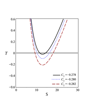
(a) $C_{2}=-0.069$ and $\Lambda=-0.02$

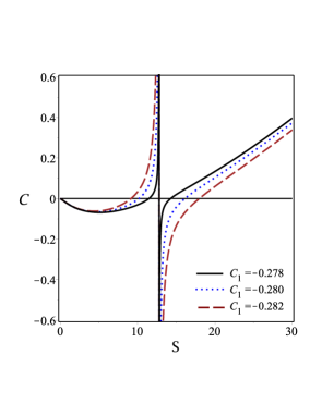
(b) $C_{2}=-0.069$ and $\Lambda=-0.02$

Figure 4: The temperature $T$ and heat capacity $C_{Q,P,C_{i}}$ versus $S$ for $Q=0.1$, $\eta=-1$, and different values of negative $C_{1}$.

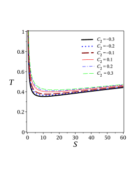
(a) $C_{1}=0.2$

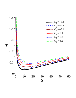
(b) $C_{1}=-0.2$

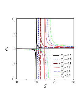
(c) $C_{1}=0.2$

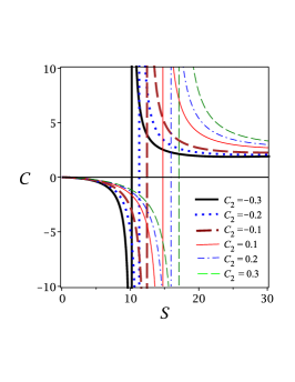
(d) $C_{1}=-0.2$

Figure 5: The temperature $T$ and heat capacity $C_{Q,P,C_{i}}$ versus $S$ for $Q=0.1$, $\eta=-1$, $\Lambda=-0.02$, and different values of negative $C_{2}$.

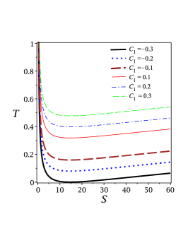
(a) $C_{2}=0.1$

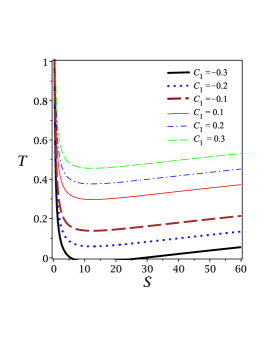
(b) $C_{2}=-0.1$

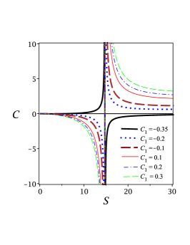
(c) $C_{2}=0.1$

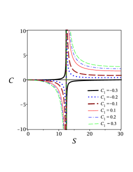
(d) $C_{2}=-0.1$

Figure 6: The temperature $T$ and heat capacity $C_{Q,P,C_{i}}$ versus $S$ for $Q=0.1$, $\eta=-1$, $\Lambda=-0.02$, and different values of negative $C_{1}$.

It seems that the obtained heat capacity in Eq. (38), may have a few physical limitation points. For this purpose, and also to understand the effects of various parameters on these points, we plot the heat capacity and the temperature in Figs. (4), (5), and (6). We can find different behavior for the physical limitation points in these figures, which depend on the parameters of our system. For example, by adjusting the parameters, we can find two physical limitation points in Fig. 4(a), or no point in the top panels of Fig. 5.

To study the behavior of the temperature (36), we expand it for small and large values of entropy in the following forms

$$\underset{S\rightarrow 0}{\lim}T \propto \frac{-\pi\eta Q^{2}}{2S^{3/2}},$$ (41)

$$\underset{S\rightarrow\infty}{\lim}T \propto 4P\sqrt{S},$$ (42)

where confirms that the temperature is always positive for small and large phantom AdS black holes because $\eta=-1$. It is worthwhile to mention that for medium black holes, the temperature is dependent on parameters $C_{1}$ and $C_{2}$ $\left(T\propto\frac{1+C_{2}+2C_{1}\sqrt{S}}{8\pi\sqrt{S}}\right)$. This relation determines that the temperature can be positive or negative. The temperature of medium phantom AdS black holes is negative (positive) when $C_{1}<\frac{-\left(1+C_{2}\right)}{2\sqrt{S}}$ $\left(C_{1}>\frac{-\left(1+C_{2}\right)}{2\sqrt{S}}\right)$. Therefore, we find two different behaviors for the temperature, which are:

i) by considering $C_{1}<\frac{-\left(1+C_{2}\right)}{2\sqrt{S}}$, the phantom AdS black holes with medium size cannot be physical objects because the temperature is negative. However, small and large black holes are physical objects (see Fig. 4(a) and black continuous line of Fig. 6(b)).

ii) according to this fact that the temperature is always positive when $C_{1}>\frac{-\left(1+C_{2}\right)}{2\sqrt{S}}$, so the phantom AdS black holes with different sizes are physical objects (see Figs. (5) and (6)).

Our results indicate that only for specific values of the parameters $C_{1}$ and $C_{2}$, small (large) phantom AdS black holes are thermally stable (unstable) (see black continuous lines of Figs. 6(c) and 6(d)); otherwise, they are thermally unstable (stable) (see down panels of Figs. (5) and (6)).

Another result is related to the effect of parameter $C_{2}$ on the local stability area of these black holes. From the down panels of Fig. 5, one can find that the local stability area decreases by increasing $C_{2}$ from $-0.3$ to $0.3$.

IV.3 Global thermal stability in grand canonical ensemble

The idea of studying the black hole’s global stability was first suggested by Hawking and Page Hawking:1983 . According to their suggestion, the black hole’s global stability can be examined in the grand canonical ensemble by calculating the Gibbs free energy, such that a black hole is globally stable provided that its Gibbs free energy is positive Dehghani2019 ; Dehghani2020 . In this subsection, we want to study the global stability of phantom AdS black holes in the context of massive gravity by using the Gibbs free energy approaches.

In the case under consideration, the Gibbs free energy can be defined via the following relation

$$G=M\left(S,Q,P,C_{i}\right)-TS-QU,$$ (43)

where, we can get the free energy by using Eqs. (35) and (36), which leads to

$$G=\frac{-32\pi PS^{2}+3\left(1+C_{2}\right)S+12\pi^{2}Q^{2}(3\eta-4)}{24\pi\sqrt{S}},$$ (44)

and we obtain the roots of free energy by solving $F=0$ that are

$$\left\{\begin{array}[]{c}S_{G_{1}}=\frac{3\left(1+C_{2}\right)-\sqrt{9\left(1+C_{2}\right)^{2}+512P\pi^{3}Q^{2}\left(9\eta-12\right)}}{64\pi P}\\ \\ S_{G_{2}}=\frac{3\left(1+C_{2}\right)+\sqrt{9\left(1+C_{2}\right)^{2}+512P\pi^{3}Q^{2}\left(9\eta-12\right)}}{64\pi P}\end{array}\right..$$ (45)

To study the behavior of the Gibbs free energy (Eq. (44)), we expand it versus $S$ in the following form

$$G=\frac{\pi Q^{2}\left(3\eta-4\right)}{2\sqrt{S}}+\frac{\left(1+C_{2}\right)\sqrt{S}}{8\pi}-\frac{4PS^{3/2}}{3},$$ (46)

the free energy is only dependent on one of the parameters of massive gravity, i.e., $C_{2}$. In addition, the Gibbs free energy for small and large values of entropy depends on

$$\underset{S\rightarrow 0}{\lim}G \propto \frac{\pi Q^{2}\left(3\eta-4\right)}{2\sqrt{S}},$$ (47)

$$\underset{S\rightarrow\infty}{\lim}G \propto -\frac{4PS^{3/2}}{3},$$ (48)

where indicates $G$ is always negative for very small and large phantom AdS black holes. So there are two global instability areas. To study the behavior of free energy carefully, we plot it versus $S$ in Fig. 7 for different values of $C_{2}$.

Briefly, our results reveal that there are three (un)stable areas (two unstable areas and one stable area):

i) the global instability areas are located in the range $S<$ $S_{G_{1}}$ because $G<0$.

ii) in the range $S_{G_{1}}<S<$ $S_{G_{2}}$, the Gibbs free energy is positive and the phantom AdS black holes satisfy the global stability condition.

iii) the Gibbs free energy is negative in the range $S>$ $S_{G_{2}}$, so the large phantom AdS black holes are unstable.

(a) $C_{1}=0.2$

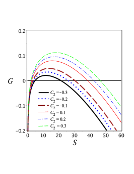
(b) $C_{1}=-0.2$

Figure 7: The Gibbs free energy ($G$) versus $S$ for $Q=0.1$, $\eta=-1$, and $\Lambda=-0.02$.

Notably, the massive parameter $C_{2}$ changes the global stability area in such a way that the global stability area increases by increasing $C_{2}$ from $-0.3$ to $0.3$ (see Fig. 7).

As a result, very small and large phantom AdS black holes are physical objects all the time; whereas medium black holes can be physical/nonphysical depending on the values of parameters. As was shown in Fig. 4, medium black holes are nonphysical only for very specific values of massive parameters. From the local stability point of view, small (large) black holes are unstable (stable) except for very specific values of massive parameters for which small (large) black holes are stable (unstable). From a global stability perspective, very small and large phantom AdS black holes are globally unstable all the time, whereas medium black holes are globally stable.

Before ending this section, we would like to examine the effect of graviton mass on thermodynamic quantities. Using definition $C_{1}=m_{g}^{2}cc_{1}$, and $C_{2}=m_{g}^{2}c^{2}c_{2}$, one can explore the effect of graviton mass on the temperature, heat capacity, and free energy. For fixed $c$, $c_{1}$, and $c_{2}$, an increase in $C_{1}$ and $C_{2}$ is equivalent to an increase in the graviton mass. From Fig. 5(b), it can be seen that the temperature increases by increasing $C_{2}$ from $0.1$ to $0.3$, meaning that increasing graviton mass leads to increasing the temperature. Also, Fig. 5(d) shows that divergence shifts to the larger entropy with an increase in the graviton mass. It reveals the fact that the phase transition takes place in larger entropy in the presence of more massive gravitons. Regarding the influence of the graviton mass on the free energy, it is clear from Fig. 6 that the graviton mass increases the free energy. In fact, increasing $m_{g}$ makes increasing the region of global stability.

V Optical Properties

In this section, we perform an in-depth study of the optical features of phantom AdS black holes in massive gravity, given by the solution (16), such as the shadow, energy emission rate, and deflection angle. Taking into account these optical quantities, we explore how the parameters of the model affect these quantities.

V.1 Photon Sphere and Shadow

Here, we intend to analyze the motion of a free photon in the black hole background (16). We first obtain the radius of the photon sphere and the shadow of the corresponding black hole, and then find admissible regions of the black hole parameters for which an acceptable optical result can be observed.

Lagrangian governing the motion of the photon is Wei104027

$$2\mathcal{L} = g_{\mu\nu}\dot{x}^{\mu}\dot{x}^{\nu},$$

$$\dot{x}^{\mu} = \frac{dx^{\mu}}{d\lambda},$$

where $\lambda$ is the affine parameter along the geodesics. Since the black hole solution (16) is spherically symmetric, we consider photons orbiting around the black hole on the equatorial hyperplane with $\theta=\pi/2$, without a significant loss of generality. So Eq. (LABEL:Lagrangian) takes the following form

$$2\mathcal{L}=-\psi(r)\dot{t}^{2}+\frac{\dot{r}^{2}}{\psi(r)}+r^{2}\dot{\phi}^{2}.$$ (50)

From the Lagrangian, we can obtain the equations of motion as

$$\dot{t} = -\frac{p_{t}}{\psi(r)},$$

$$\dot{r} = p_{r}\psi(r),$$ (51)

$$\dot{\varphi} = \frac{p_{\varphi}}{r^{2}},$$

where $p$ is the generalized momentum defined by $p_{\mu}=\partial\mathcal{L}/\partial\dot{x}^{\mu}=g_{\mu\nu}\dot{x}^{\nu}$.

According to Eqs. (7) and (16), the coefficients are independent of ”$t$” and ”$\varphi$”. So, one can consider $p_{t}\equiv-E$ and $p_{\varphi}\equiv L$ as constants of motion, where $E$ and $L$ are the energy and angular momentum of the photon, respectively. Using the equations of motion and two conserved quantities, one can rewrite the null geodesic equation as follows

$$\dot{r}^{2}+V_{\mathrm{eff}}(r)=0,$$ (52)

where the effective potential $V_{\mathrm{eff}}$ is

$$V_{\mathrm{eff}}(r)=\psi(r)\left[\frac{L^{2}}{r^{2}}-\frac{E^{2}}{\psi(r)}\right].$$ (53)

To have the spherical geodesics, we apply two conditions

$$V_{\mathrm{eff}}(r)|_{r=r_{ph}} = 0,$$

$$\frac{\partial V_{\mathrm{eff}}(r)}{\partial r}\Big{|}_{r=r_{ph}} = 0,$$

where $r_{ph}$ is the radius of photon sphere. With the use of Eq. (53), solving $V_{eff}^{\prime}(r_{ph})=0$ leads to the following relation

$$C_{1}r_{ph}^{3}+4(C_{2}+1)r_{ph}^{2}-12m_{0}r_{ph}-8q^{2}=0,$$ (55)

as we see, Eq. (55) is cubic in $r_{ph}$ and its discriminant $\Delta$ can be calculated as

$$\Delta=\frac{P^{3}}{27}+\frac{\mathcal{Q}^{2}}{4},$$ (56)

in which $P$ and $Q$ are given by

$$P = -\frac{12m_{0}}{C_{1}}-\frac{16(C_{2}+1)^{2}}{3C_{1}^{2}},$$ (57)

$$\mathcal{Q} = -\frac{8q^{2}}{C_{1}}+\frac{16m_{0}(C_{2}+1)}{C_{1}^{2}}+\frac{128(C_{2}+1)^{3}}{27C_{1}^{3}}.$$ (58)

Depending on the values of the black hole parameters, $\Delta$ can be positive or negative. Fig. 8 displays positive/negative regions of $\Delta$, giving us a more precise picture of this function. For the case of positive $\Delta$, we will have only one real solution defined as

$$r_{ph}=\left(-\frac{q}{2}+\sqrt{\Delta}\right)^{\frac{1}{3}}+\left(-\frac{q}{2}-\sqrt{\Delta}\right)^{\frac{1}{3}}-\frac{2}{3}\frac{(1+C_{2})}{C_{1}}.$$ (59)

For $\Delta<0$, there are three real solutions which are determined as

$$r_{ph}^{(1)} = \frac{2\sqrt{-P}\sin\left[\frac{\sin^{-1}\left(\frac{3\sqrt{3}\mathcal{Q}}{2(\sqrt{-P})^{3}}\right)}{3}\right]}{\sqrt{3}}-\frac{2(1+C_{2})}{3C_{1}},$$ (60)

$$r_{ph}^{(2)} = -\frac{2\sqrt{-P}\sin\left[\frac{\sin^{-1}\left(\frac{3\sqrt{3}\mathcal{Q}}{2(\sqrt{-P})^{3}}\right)}{3}+\frac{\pi}{3}\right]}{\sqrt{3}}-\frac{2(1+C_{2})}{3C_{1}},$$ (61)

$$r_{ph}^{(3)} = \frac{2\sqrt{-P}\cos\left[\frac{\sin^{-1}\left(\frac{3\sqrt{3}\mathcal{Q}}{2(\sqrt{-P})^{3}}\right)}{3}+\frac{\pi}{6}\right]}{\sqrt{3}}-\frac{2(1+C_{2})}{3C_{1}}.$$ (62)

According to our analysis, $r^{(3)}_{ph}$ given by Eq. (63) is the largest positive root. From the first condition of Eq.(LABEL:Eqcondition), the shadow radius can be obtained as Perlick104031

$$r_{sh}=\frac{L_{p}}{E}=\frac{r_{ph}}{\sqrt{\psi(r_{ph})}}.$$ (63)

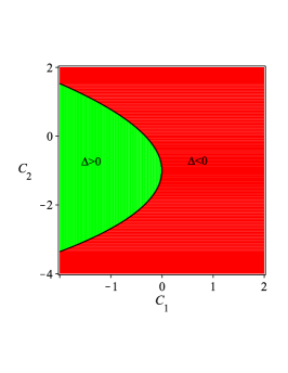
(a) $q=0.5$

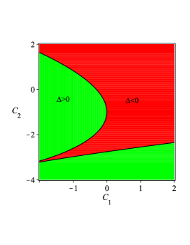
(b) $q=0.8$

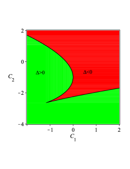
(c) $q=0.9$

Figure 8: Positive or negative regions of discriminant $\Delta$ for $\eta=-1$ and $m_{0}=1$.

The apparent shape of a shadow can be obtained by a stereo-graphic projection in terms of the celestial coordinates $x$ and $y$ which are defined as Vazquez489

$$x = \lim_{r_{0}\rightarrow\infty}\left(-r_{0}^{2}\sin\theta_{0}\frac{d\varphi}{dr}\Big{|}_{(r_{0},\theta_{0})}\right),$$

$$y = \lim_{r_{0}\rightarrow\infty}\left(r_{0}^{2}\frac{d\theta}{dr}\Big{|}_{(r_{0},\theta_{0})}\right),$$

where $r_{0}$ is the distance between the observer and the black hole, and $\theta_{0}$ is the inclination angle.

Table 1: The event horizon ($r_{e}$), photon sphere radius ($r_{ph}$) and shadow radius ($r_{sh}$) for the variation of $q$, $C_{1}$, $C_{2}$ and $\Lambda$ for $\eta=-1$ and $m_{0}=1$.

$q$	$0.1$	$0.4$	$0.7$	$1.2$
$r_{e}$ ($C_{1}=0.5$, $C_{2}=0.2$ and $\Lambda=-0.02$)	$1.3055$	$1.3632$	$1.4735$	$1.7198$
$r_{ph}$ ($C_{1}=0.5$, $C_{2}=0.2$ and $\Lambda=-0.02$)	$2.0642$	$2.1450$	$2.3044$	$2.7194$
$r_{sh}$ ($C_{1}=0.5$, $C_{2}=0.2$ and $\Lambda=-0.02$)	$2.3474$	$2.3985$	$2.4975$	$2.6627$
$r_{ph}>r_{e}$	✓	✓	✓	✓
$r_{sh}>r_{ph}$	✓	✓	✓	$\times$
$C_{1}$	$-0.4$	$-0.01$	$0.1$	$0.82$
$r_{e}$ ($q=0.5$, $C_{2}=0.2$ and $\Lambda=-0.02$)	$22.6371$	$1.7669$	$1.6536$	$1.2691$
$r_{ph}$ ($q=0.5$, $C_{2}=0.2$ and $\Lambda=-0.02$)	$8.3236$	$45.3448$	$2.5311$	$2.0092$
$r_{sh}$ ($q=0.5$, $C_{2}=0.2$ and $\Lambda=-0.02$)	$-16.7572$	$12.7763$	$3.4441$	$2.0058$
$r_{ph}>r_{e}$	$\times$	✓	✓	✓
$r_{sh}>r_{ph}$	$\times$	$\times$	✓	$\times$
$C_{2}$	$-0.4$	$0.1$	$0.5$	$1.1$
$r_{e}$ ( $C_{1}=q=0.5$ and $\Lambda=-0.02$)	$1.9255$	$1.4658$	$1.1653$	$0.9628$
$r_{ph}$ ($C_{1}=q=0.5$ and $\Lambda=-0.02$)	$3.1697$	$2.3147$	$1.7967$	$1.4658$
$r_{sh}$ ($C_{1}=q=0.5$ and $\Lambda=-0.02$)	$3.5360$	$2.5819$	$1.9151$	$1.4637$
$r_{ph}>r_{e}$	✓	✓	✓	✓
$r_{sh}>r_{ph}$	✓	✓	✓	$\times$
$\Lambda$	$-0.01$	$-0.05$	$-0.09$	$-0.14$
$r_{e}$ ($C_{1}=q=0.5$ and $C_{2}=0.2$)	$1.3997$	$1.3824$	$1.3663$	$1.3476$
$r_{ph}$ ($C_{1}=q=0.5$ and $C_{2}=0.2$)	$2.1904$	$2.1904$	$2.1904$	$2.1904$
$r_{sh}$ ($C_{1}=q=0.5$ and $C_{2}=0.2$)	$2.4513$	$2.3587$	$2.2758$	$2.1835$
$r_{ph}>r_{e}$	✓	✓	✓	✓
$r_{sh}>r_{ph}$	✓	✓	✓	$\times$

Now with $r_{ph}$ and $r_{sh}$ in hand, we can investigate allowed regions of the parameters to have acceptable optical behavior. To do so, we need to investigate the condition $r_{e}<r_{ph}<r_{sh}$, where $r_{e}$ is the radius related to the event horizon. For clarity, we list several values of the event horizon, the photon sphere radius, and the shadow radius in table 1. As we see, for large values of the electric charge, the cosmological constant, and parameters $C_{1}$ and $C_{2}$, the shadow size is smaller than the photon sphere radius, which is not acceptable physically. As a remarkable point regarding the parameter $C_{1}$, we notice that an acceptable optical result can be observed just for positive values of this parameter. From this table, one can also see how the event horizon, photon sphere radius, and shadow size change by varying the parameters of the model. Studying the effect of electric charge on these quantities, we find that the increase of this parameter leads to the increase of all three quantities. Regarding the effect of the cosmological constant and parameters $C_{1}$ and $C_{2}$, our analysis shows that these parameters have decreasing contributions to the event horizon, the photon sphere radius, and the shadow radius. To better understand the effect of these parameters on the shadow size, we have plotted Fig. 9. From this figure, it is clear that the influence of parameters $C_{1}$ and $C_{2}$ on the size of the black hole shadow is significant compared to the electric charge and the cosmological constant. As was already mentioned, for fixed $c$, $c_{1}$, and $c_{2}$, the change of $C_{1}$ and $C_{2}$ shows the variation of the massive graviton. Therefore, Fig. 9(a) represents the increasing contribution of the graviton mass on the shadow size.

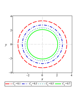
(a) $q=C_{2}=0.2$ and $\Lambda=-0.02$

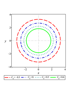
(b) $C_{1}=0.5$, $q=0.2$ and $\Lambda=-0.02$

(c) $C_{1}=0.5$, $C_{2}=0.2$ and $\Lambda=-0.02$

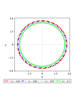
(d) $C_{1}=0.5$ and $q=C_{2}=0.2$

Figure 9: The black hole shadow in the celestial plane $(x-y)$ for $\eta=-1$ and $m_{0}=1$.

V.2 Energy emission

Having the black hole shadow, it is possible to study the emission of particles around the black hole. It has been known that the black hole shadow corresponds to its high energy absorption cross-section for the observer located at infinity Wei063 . In fact, the absorption cross-section oscillates around a limiting constant value $\sigma_{lim}$ for a spherically symmetric black hole. Since the shadow measures the optical appearance of a black hole, it is approximately equal to the area of the photon sphere ($\sigma_{lim}\approx\pi r_{sh}^{2}$). For $4-$dimensional spacetime, the energy emission rate is defined as

$$\frac{d^{2}\mathcal{E}(\omega)}{dtd\omega}=\frac{2\pi^{3}\omega^{3}r_{sh}^{2}}{e^{\frac{\omega}{T}}-1},$$ (65)

in which $\omega$ and $T$ are, respectively, the emission frequency and Hawking temperature. Inserting Eq. (23) into Eq. (65), the energy emission rate can be obtained for the present black hole solution. In Figure 10, these energetic aspects are plotted as a function of the emission frequency for different values of the electric charge, cosmological constant, and parameters $C_{1}$ and $C_{2}$. As it is transparent, there exists a peak of the energy emission rate, which decreases and shifts to low frequencies as the parameters $C_{1}$, $C_{2}$, $q$, and $|\Lambda|$ decrease. From this figure, all four parameters have an increasing effect on the emission rate. This shows that as the influence of these parameters becomes stronger, the evaporation process becomes faster. As a result, the black hole has a shorter lifetime in the presence of the more massive gravitons and strong electric fields, or a high curvature background.

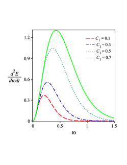
(a) $q=C_{2}=0.2$ and $\Lambda=-0.02$

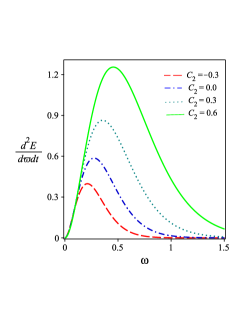
(b) $C_{1}=0.5$, $q=0.2$ and $\Lambda=-0.02$

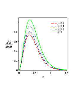
(c) $C_{1}=0.5$, $C_{2}=0.2$ and $\Lambda=-0.02$

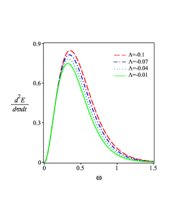
(d) $C_{1}=0.5$ and $q=C_{2}=0.2$

Figure 10: The energy emission rate versus $\omega$ for the corresponding black hole with $\eta=-1$, $m_{0}=1$ and different values of $C_{1}$, $C_{2}$, $q$ and $\Lambda$.

V.3 Deflection Angle

Gravitational lensing is a subject of wide interest that has a tremendous impact on the distribution of matters and the constituents of the Universe. The gravitational lensing effect states that a light beam is distorted when it passes through a huge object, which is one of the most important predictions of general relativity. The deflection of light by gravitational fields has been studied with great interest in astrophysics as well as in theoretical physics. Determining the mass of galaxies and clusters Henk177 ; Brouwer481 , as well as discovering dark energy and dark matter Vanderveld103518 is an important application of gravitational lensing in astronomy and cosmology. In this subsection, we employ the Gauss-Bonnet theorem and study the light deflection around the black hole solution (16). We exploit the optical geometry of the black hole solution and find the Gaussian curvature in weak gravitational lensing.

Using weak field approximation, the Gauss-Bonnet theorem in optical metric can be expressed as follows Gibbons2350 ; Werner3047 ; Jusufi8403

$$\int\int_{\mathcal{D}_{R}}\mathcal{K}dS+\oint_{\partial\mathcal{D}_{R}}kdt+\sum_{i}\theta_{i}=2\pi\mathcal{X}(\mathcal{D}_{R}),$$ (66)

where $D_{R}$ is a region consisting of the source of light waves, the observer, and the focal point of the lens. $\mathcal{K}$ and $k$ are, respectively, the Gaussian curvature of $D_{R}$ and the geodesic curvature of $\partial\mathcal{D}_{R}$. Also, $dS$ is the area element and $\theta_{i}$ refers to the exterior angle at the $i-th$ vertex.

As the light beam approaches from infinity up to a large distance, and since we are working with weak field limitations, the light beam is almost straight. So, we employ the straight-line approximation $r=\frac{b}{sin(\varphi)}$, where $b$ is the impact parameter. With this, the asymptotic deflection angle $\alpha$ can be calculated as Gibbons2350 ; Jusufi8403 ; Kumaran2210

$$\alpha=-\int_{0}^{\pi}\int_{\frac{b}{\sin\phi}}^{\infty}\mathcal{K}dS.$$ (67)

To calculate the deflection angle, we need to determine the optical path, which is obtained by the null geodesic condition $ds^{2}=0$. Since we have considered the motion of photon in the equatorial plane ($\theta=\pi/2$), the optical path metric can be obtained as

$$dt^{2}=\tilde{g}_{ij}dx^{i}dx^{j}=\frac{1}{\psi^{2}(r)}dr^{2}+\frac{r^{2}}{\psi(r)}d\varphi^{2}.$$ (68)

To obtain the optical Gaussian curvature $\mathcal{K}$ from the optical metric Equation (68), we use the expression $\mathcal{K}=R/2$ Upadhyay2210 , in which $R$ is the Ricci scalar calculated using the optical metric. Here, the infinitesimal surface element can be computed as Upadhyay2210

$$dS=\sqrt{det\left(\tilde{g}\right)}drd\varphi=\frac{r}{\psi(r)^{3/2}}drd\varphi.$$ (69)

Using Equation (67) and the value of optical Gaussian curvature, the deflection angle $\alpha$ of the corresponding black hole is calculated as

$$\alpha \simeq \frac{3\sqrt{3}\pi\left(9C_{1}^{3}+48C_{1}\Lambda(C_{2}+1)-128m_{0}\Lambda^{2}\right)}{256b^{2}\left(-\Lambda\right)^{\frac{5}{2}}}+\frac{\sqrt{3}\left(48\Lambda(C_{2}+1)^{2}+9C_{1}^{2}(C_{2}+1)\right)}{24b^{3}\left(-\Lambda\right)^{\frac{5}{2}}}+\frac{1701\sqrt{3}\pi m_{0}q^{4}}{512b^{10}\left(-\Lambda\right)^{\frac{5}{2}}}$$

$$+\frac{45\sqrt{3}\pi\left(\left(9C_{1}^{2}-32\Lambda(C_{2}+1)\right)m_{0}-8\Lambda C_{1}q^{2}\right)}{512b^{4}\left(-\Lambda\right)^{\frac{5}{2}}}-\frac{\sqrt{3}\left(96\Lambda m_{0}C_{1}+64\Lambda^{2}q^{2}\right)}{24b^{3}\left(-\Lambda\right)^{\frac{5}{2}}}+\frac{1536\sqrt{3}q^{6}}{847b^{11}\left(-\Lambda\right)^{\frac{5}{2}}}$$

$$+\frac{128\sqrt{3}q^{2}\left(3m_{0}^{2}-(C_{2}+1)q^{2}\right)}{21b^{9}\left(-\Lambda\right)^{\frac{5}{2}}}+\frac{2\sqrt{3}\Lambda\left(C_{1}^{2}+(C_{2}+1)\Lambda\right)}{3b\left(-\Lambda\right)^{\frac{5}{2}}}+\frac{3\sqrt{3}\left(\left(16\Lambda(C_{2}+1)+9C_{1}^{2}\right)q^{2}\right)}{10b^{5}\left(-\Lambda\right)^{\frac{5}{2}}}$$

$$+\frac{3\sqrt{3}\left(32\Lambda m_{0}^{2}+24C_{1}m_{0}(C_{2}+1)\right)}{10b^{5}\left(-\Lambda\right)^{\frac{5}{2}}}+\frac{15\sqrt{3}\pi\left(21C_{1}q^{2}(C_{2}+1)-27C_{1}m_{0}^{2}\right)}{128b^{6}\left(-\Lambda\right)^{\frac{5}{2}}}$$

$$+\frac{15\sqrt{3}\pi\left(\left(28\Lambda q^{2}+12(C_{2}+1)^{2}\right)m_{0}\right)}{128b^{6}\left(-\Lambda\right)^{\frac{5}{2}}}-\frac{24\sqrt{3}\left(126m_{0}^{2}(C_{2}+1)+153m_{0}C_{1}q^{2}\right)}{245b^{7}\left(-\Lambda\right)^{\frac{5}{2}}}$$

$$+\frac{24\sqrt{3}\left(2q^{2}\left(14\Lambda q^{2}+27(C_{2}+1)^{2}\right)\right)}{245b^{7}\left(-\Lambda\right)^{\frac{5}{2}}}-\frac{945\sqrt{3}\pi\left(3C_{1}q^{4}-6m_{0}^{3}+14m_{0}q^{2}(C_{2}+1)\right)}{2048b^{8}\left(-\Lambda\right)^{\frac{5}{2}}},$$

The behavior of $\alpha$ concerning the impact parameter, $b$, is illustrated in Figure 11. As we see, for small (large) values of the parameter $C_{1}$ ($|\Lambda|$), the deflection angle is a decreasing function of $b$. Otherwise, $\alpha$ behavior is slightly different in such a way that the deflection angle first decreases to a minimum value with the increase of $b$, then increases and reaches a maximum value with the further increase of the impact parameter, after that, it gradually decreases as $b$ goes to infinity. Fig. 11 also shows how $\alpha$ changes by varying black hole parameters. According to Fig. 11(a), the parameter $C_{1}$ has a decreasing contribution to the deflection angle. For fixed $c$, $c_{1}$, and $c_{2}$, this is equivalent to the decreasing effect of the graviton mass on the deflection angle. In contrast to $C_{1}$, the parameter $C_{2}$ has an increasing effect on $\alpha$ (see Fig. 11(b)). Regarding the electric charge effect, we see from Fig. 11(c), that its effect is similar to that of the parameter $C_{1}$. But as it is clear, its effect is insignificant compared to other parameters, indicating that variation of the electric charge does not have a remarkable effect on the deflection angle. Analyzing Fig. 11(d) we find that for intermediate values of the impact parameter, $\alpha$ is an increasing function of the cosmological constant, whereas, for large values of $b$, it is a decreasing function of $\Lambda$. This reveals the fact that photons with large angular momentum deviate much more from their straight path in a low-curvature background.

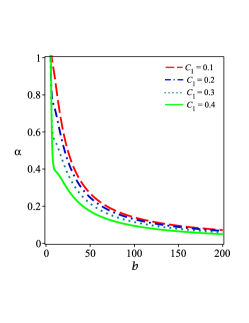
(a) $q=C_{2}=0.2$ and $\Lambda=-0.08$

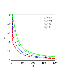
(b) $q=C_{1}=0.2$ and $\Lambda=-0.08$

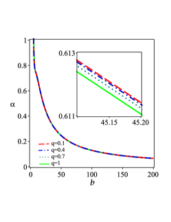
(c) $C_{1}=C_{2}=0.2$ and $\Lambda=-0.08$

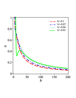
(d) $C_{1}=C_{2}=q=0.2$

Figure 11: The behavior of $\alpha$ with respect to the impact parameter $b$ for $\eta=-1$, $m_{0}=1$ and different values of $C_{1}$, $C_{2}$, $q$ and $\Lambda$.

VI Quasinormal Modes

From a theoretical point of view, perturbations of a black hole’s spacetime can be performed in two ways: by perturbing the black hole metric (the background) or by adding fields to the black hole’s spacetime. When black holes are perturbed, they tend to relax toward equilibrium. Such a process is done through the emission of QNMs. QNMs are complex frequencies, $\omega=\omega_{R}-i\omega_{I}$, which encode important information related to the stability of the black hole under small perturbations. The sign of the imaginary part determines if the mode is stable or unstable. For positive $\omega_{I}$ the mode is unstable, whereas negativity represents stable modes. For a stable mode, the real part provides the frequency of the oscillation, while the inverse of $|Im(\omega)|$ determines the damping time $t_{D}^{-1}=|Im(\omega)|$ Blazquez2020 . There are some types of perturbation such as scalar, Dirac, vector, or tensor. In this paper, we are interested in investigating scalar perturbations by a massive field around a black hole.

Massive Scalar Perturbations: Here, we will study the QN frequencies of a massive scalar field. For a scalar field $\Psi$ of mass $\mu$ in the background of the metric $g_{\mu\nu}$, the equation of motion is given by the following Klein-Gordon equation

$$(\nabla^{\nu}\nabla_{\nu}-\mu^{2})\Psi=0,$$ (70)

where $\nabla_{\nu}$ is the covariant derivative. The above equation can be written explicitly as follows:

$$\frac{1}{\sqrt{-g}}\partial_{\nu}(\sqrt{-g}g^{\mu\nu}\partial_{\mu}\Psi)-\mu^{2}\Psi=0.$$ (71)

Using the method of separation of variables, the scalar field can be written as

$$\Psi(t,r,\theta,\phi)=\frac{u_{L}(r)}{r}e^{-i\omega t}Y_{Lm}(\theta,\phi),$$ (72)

which $Y_{lm}(\theta,\phi)$ denotes the spherical harmonics and the function $u_{l}(r)$ satisfies an ordinary second order linear differential equation as follows

$$\frac{d^{2}u_{l}}{dx^{2}}+\left[\omega^{2}-V(r)\right]u_{l}=0,$$ (73)

where $x=\int\frac{dr}{\psi(r)}$ represents the tortoise coordinates. The corresponding effective potential barrier is given by

$$V_{l}(r)=\psi(r)\left(\mu^{2}+\frac{l(l+1)}{r^{2}}+\frac{\psi^{\prime}(r)}{r}\right),$$ (74)

where $l$ is the multipole number.

QNMs were investigated with different methods over the last decades. Here, we employ the semi-analytical WKB approximation, which is based on the matching of the WKB expansion of the modes at the event horizon and spatial infinity with the Taylor expansion of the effective potential near the peak of the potential barrier. This method was first proposed in the 1980s SIyer ; QNM2 and then extended to 6th order QNM3 , and to 13th order Konoplya1 . It should be noted that increasing the WKB order does not always lead to a better approximation for the frequency, so we employ the 3rd order expansion for our study, which is given by the following formula

$$\omega^{2}=[V_{0}+(-2V_{0}^{{}^{\prime\prime}})^{\frac{1}{2}}\Lambda]-i\nu(-2V_{0}^{{}^{\prime\prime}})^{\frac{1}{2}}(1+\Omega),$$ (75)

where

$$\Lambda(n) = \frac{\left(\frac{V_{0}^{(4)}}{V_{0}^{{}^{\prime\prime}}}\right)\left(\frac{1}{4}+\nu^{2}\right)}{8\left(-2V_{0}^{{}^{\prime\prime}}\right)^{1/2}}-\frac{\left(\frac{V_{0}^{{}^{\prime\prime\prime}}}{V_{0}^{{}^{\prime\prime}}}\right)^{2}\left(7+60\nu^{2}\right)}{288\left(-2V_{0}^{{}^{\prime\prime}}\right)^{1/2}}\ ,$$ (76)

$$\Omega(n) = \frac{5\left(\frac{V_{0}^{{}^{\prime\prime\prime}}}{V_{0}^{{}^{\prime\prime}}}\right)^{4}(77+188\nu^{2})}{6912\left(-2V_{0}^{{}^{\prime\prime}}\right)^{1/2}}-\frac{\left(\frac{V_{0}^{{}^{\prime\prime\prime 2}}V_{0}^{(4)}}{V_{0}^{{}^{\prime\prime 3}}}\right)(51+100\nu^{2})}{384\left(-2V_{0}^{{}^{\prime\prime}}\right)^{1/2}}+\frac{\left(\frac{V_{0}^{(4)}}{V_{0}^{{}^{\prime\prime}}}\right)^{2}(67+68\nu^{2})}{2304\left(-2V_{0}^{{}^{\prime\prime}}\right)^{1/2}}$$ (77)

$$+\frac{\left(\frac{V_{0}^{{}^{\prime\prime\prime}}V_{0}^{(5)}}{V_{0}^{{}^{\prime\prime 2}}}\right)(19+28\nu^{2})}{288\left(-2V_{0}^{{}^{\prime\prime}}\right)^{1/2}}-\frac{\left(\frac{V_{0}^{(6)}}{V_{0}^{{}^{\prime\prime}}}\right)(5+4\nu^{2})}{288\left(-2V_{0}^{{}^{\prime\prime}}\right)^{1/2}}.$$

In the relations above, $\nu=n+\frac{1}{2}$ and $n$ is the overtone number. $V_{0}^{(j)}$ denotes the $j$-order derivative of the effective potential on the point maximum $x_{0}$. It is worth pointing out that the WKB formula does not give reliable frequencies for $n\geq l$, whereas it leads to quite accurate values for $n<l$. Now, using Eq. (74) and Eq. (75), we can calculate the QNMs for the corresponding black hole, which is shown in Fig. 12 with different values of black hole parameters. We see that as the parameter $C_{1}$ increases, both the real and absolute value of imaginary parts of the QN frequency grows monotonically. This shows that when this parameter gets more, the scalar perturbations oscillate more rapidly, and due to the increasing imaginary part, they decay faster. For fixed $c$, $c_{1}$, and $c_{2}$, one can also say that the scalar perturbations oscillate with more energy and decay faster in the presence of the more massive gravitons. Figs. 12(a) and 12(b) show how $Re(\omega)$ and $|Im(\omega)|$ change under varying the $C_{2}$ parameter. The curves shift upwards by increasing $C_{2}$, meaning that both real and imaginary parts of the QNMs are an increasing function of this parameter. Figs. 12(c) and 12(d) give a simple illustration of how the dependence of the QNMs on the electric charge. As we see, $q$ decreases (increases) the real (absolute value of the imaginary) part of $\omega$. This implies that the scalar field perturbations around the black hole oscillate with less energy and decay faster in a powerful electric field.

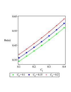
(a) $q=0.2$

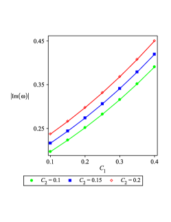
(b) $q=0.2$

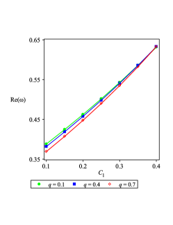
(c) $C_{2}=0.2$

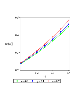
(d) $C_{2}=0.2$

Figure 12: The behavior of $Re(\omega)$ and $|Im(\omega)|$ with the parameter $C_{1}$ for $\eta=-1$, $m_{0}=1$ and different values of $C_{2}$ and $q$.

VII Conclusions

In this paper, we have obtained AdS phantom solutions in the dRGT-like massive gravity. Investigating some geometrical properties, we have shown that such solutions can be interpreted as black hole solutions. Then, we studied the thermodynamic structure of solutions in the extended phase space and examined the validity of the first law of thermodynamics. Calculating heat capacity, we investigated the local stability of the system and showed how the parameters of the model affect the region of the stability. According to our analysis, large (small) phantom AdS black holes are in a local stable (unstable) state all the time. We also examined the global stability of the system through the use of Helmholtz-free energy and found that large and small phantom AdS black holes are globally stable, whereas medium black holes cannot satisfy the global stability condition.

In the next step, we studied the optical features of black holes and noticed that some constraints should be imposed on the range of parameters of the model under consideration to have acceptable optical behavior. Studying the effect of the parameters on the size of the shadow and the radius of the photon sphere showed that the electric charge has an increasing effect on these two optical quantities, while the parameters $C_{1}$ and $C_{2}$ have a decreasing contribution to them. Regarding the cosmological constant effect, although the photon sphere radius is not affected by this parameter, the shadow size shrinks by increasing $|\Lambda|$.

We continued our investigation by studying the energy emission rate and the impact of black hole parameters on the radiation process. Our analysis showed that all parameters have an increasing contribution to the emission rate, namely, the evaporation process gets faster as the effects of these parameters get stronger. This reveals the fact that the lifetime of the black hole would be shorter with the increase of the parameters of the model.

After that, we performed an in-depth analysis of the gravitational lensing of light around such black holes. Depending on the choice of the black hole parameters, we observed different behaviors. For large (small) values of the cosmological constant (parameter $C_{1}$), the deflection angle $\alpha$ is a decreasing function of the impact parameter $b$. While for small (large) values of $|\Lambda|$ ($C_{1}$ parameter), $\alpha$ first decreases as $b$ increases, then increases and reaches a local maximum as $b$ increases further, after that, it gradually decreases as $b$ goes to infinity. Regarding the influence of parameters on $\alpha$, we found that the parameter $C_{1}$, electric charge, and the absolute value of the cosmological constant have a decreasing contribution to $\alpha$, whereas the parameter $C_{2}$ has an increasing effect. This shows that photons are more deflected in a weak electric field or when the effect of massive parameter $C_{2}$ ($C_{1}$) gets strong (weak).

Finally, we presented a study of the quasinormal modes of scalar perturbation. We found that both massive parameters $C_{1}$ and $C_{2}$ increase the real part and absolute value of the imaginary part of the quasinormal frequencies. This means that the quasinormal modes oscillate with more energy and decay faster around the black holes in the presence of massive gravity. Studying the effect of the electric charge showed that the real (imaginary) part of the quasinormal modes decreases (increases) with the growth of this parameter, indicating that the scalar field perturbations in the presence of electric charge oscillate more slowly and decay faster as compared to neutral black holes.

- (1) M. Fierz, and W. E. Pauli, Proc. Roy. Soc. Lond. A 173 (1939) 211.
- (2) A. I. Vainshtein, Phys. Lett. B 39 (1972) 393.
- (3) D. G. Boulware, and S. Deser, Phys. Rev. D 6 (1972) 3368.
- (4) E. A. Bergshoe, O. Hohm, and P. K. Townsend, Phys. Rev. Lett. 102 (2009) 201301.
- (5) C. de Rham, and G. Gabadadze, Phys. Rev. D 82 (2010) 044020.
- (6) C. de Rham, G. Gabadadze, and A. J. Tolley, Phys. Rev. Lett. 106 (2011) 231101.
- (7) K. Koyama, G. Niz, and G. Tasinato, Phys. Rev. Lett. 107 (2011) 131101.
- (8) T. M. Nieuwenhuizen, Phys. Rev. D 84 (2011) 024038.
- (9) A. Gruzinov, and M. Mirbabayi, Phys. Rev. D 84 (2011) 124019.
- (10) L. Berezhiani, G. Chkareuli, C. de Rham, G. Gabadadze, and A. J. Tolley, Phys. Rev. D 85 (2012) 044024.
- (11) M. S. Volkov, Phys. Rev. D 85 (2012) 124043.
- (12) P. Gratia, W. Hu, and M. Wyman, Phys. Rev. D 86 (2012) 061504.
- (13) C. -I. Chiang, K. Izumi, and P. Chen, J. Cosmol. Astropart. Phys. 1212 (2012) 025.
- (14) E. Babichev, and A. Fabbri, Class. Quantum Gravit. 30 (2013) 152001.
- (15) R. Brito, V. Cardoso, and P. Pani, Phys. Rev. D 88 (2013) 064006.
- (16) H. Kodama, and I. Arraut, Prog. Theor. Exp. Phys. 2014 (2014) 023E02.
- (17) S. Renaux-Petel, J. Cosmol. Astropart. Phys. 1403 (2014) 043.
- (18) E. Babichev, and A. Fabbri, Phys. Rev. D 89 (2014) 081502.
- (19) S. G. Ghosh, L. Tannukij, and P. Wongjun, Eur. Phys. J. C 76 (2016) 1
- (20) B. Eslam Panah, S. H. Hendi, and Y. C. Ong, Phys. Dark Universe. 27 (2020) 100452.
- (21) S. H. Hendi, Kh. Jafarzade, and B. Eslam Panah, J. Cosmol. Astropart. Phys. 02 (2023) 022.
- (22) T. Q. Do, Phys. Rev. D 93 (2016) 104003.
- (23) T. Q. Do, Phys. Rev. D 94 (2016) 044022.
- (24) D. Comelli, M. Crisostomi, F. Nesti, and L. Pilo, J. High Energy Phys. 3 (2012) 1.
- (25) D. Langlois, and A. Naruko, Class. Quantum Gravit. 29 (2012) 202001.
- (26) T. Kobayashi, M. Siino, M. Yamaguchi, and D. Yoshida, Phys. Rev. D 86 (2012) 061505.
- (27) A. De Felice, A. E. Gumrukcuoglu, C. Lin, and S. Mukohyama, Class. Quantum Gravit. 30 (2013) 184004.
- (28) K. Hinterbichler, and R. A. Rosen, J. High Energy Phys. 7 (2012) 1.
- (29) S. F. Hassan, and R. A. Rosen, J. High Energy Phys. 2 (2012) 1.
- (30) D. Vegh, ”Holography without translational symmetry”, [arXiv:1301.0537].
- (31) R. -G. Cai, Y. -P. Hu, Q. -Y. Pan, and Y. -L. Zhang, Phys. Rev. D 91 (2015) 024032.
- (32) S. H. Hendi, B. Eslam Panah, and S. Panahiyan, J. High Energy Phys. 11 (2015) 157.
- (33) S. H. Hendi, B. Eslam Panah, and S. Panahiyan, Class. Quantum Gravit. 33 (2016) 235007.
- (34) S. H. Hendi, B. Eslam Panah, and S. Panahiyan, Phys. Lett. B 769 (2017) 191.
- (35) S. H. Hendi, G. -Q. Li, J. -X. Mo, S. Panahiyan, and B. Eslam Panah, Eur. Phys. J. C 76 (2016) 571.
- (36) Y. -B. Ma, R. Zhao, and S. Cao, Commun. Theor. Phys. 69 (2018) 544.
- (37) Y. Ma, et al., Eur. Phys. J. C 80 (2020) 213.
- (38) B. Wu, C. Wang, Z. M. Xu, and W. L. Yang, Eur. Phys. J. C 81 (2021) 626.
- (39) B. Eslam Panah, Kh. Jafarzade, and A. Rincon, [arXiv:2201.13211].
- (40) P. Paul, S. Upadhyay, and D. V. Singh, Eur. Phys. J. Plus. 138 (2023) 566.
- (41) B. Eslam Panah, and S. H. Hendi, Europhys. Lett. 125 (2019) 60006.
- (42) S. H. Hendi, G. H. Bordbar, B. Eslam Panah, and S. Panahiyan, J. Cosmol. Astropart. Phys. 07 (2017) 004.
- (43) B. Eslam Panah, and H. L. Liu, Phys. Rev. D 99 (2019) 104074.
- (44) A. Bagheri Tudeshki, G. H. Bordbar, and B. Eslam Panah, Phys. Dark Universe. 42 (2023) 101354.
- (45) S. H. Hendi, R. B. Mann, S. Panahiyan, and B. Eslam Panah, Phys. Rev. D 95 (2017) 021501(R).
- (46) M. Visser, Lorenzian Wormholes: from einstein to Hawking, Spring Verlag, New York (1996).
- (47) R. R. Caldwell, M. Kamionkowski, and N. N. Weinberg, Phys. Rev. Lett. 91 (2003) 071301.
- (48) A. Einstein, and N. Rosen, Phys. Rev. 48 (1935) 73.
- (49) K. A. Bronnikov, M. S. Chernakova, J. C. Fabris, N. Pinto-Neto, and M. E. Rodrigues, Int. J. Mod. Phys. D 17 (2008) 25.
- (50) G. Clement, J. C. Fabris, and M. E. Rodrigues, Phys. Rev. D 79 (2009) 064021.
- (51) D. F. Jardim, M. E. Rodrigues, and S. J. M. Houndjo, Eur. Phys. J. Plus 127 (2012) 123.
- (52) K. A. Bronnikov, and J. C. Fabris, Phys. Rev. Lett. 96 (2006) 251101.
- (53) M. Azreg-Ainou, G. Clement, J. C. Fabris, and M. E. Rodrigues, Phys. Rev. D 83 (2011) 124001.
- (54) M. Azreg-Ainou, Phys. Rev. D 87 (2013) 024012.
- (55) A. Nakonieczna, M. Rogatko, and R. Moderski, Phys. Rev. D 86 (2012) 044043.
- (56) G. N. Gyulchev, and I. Z. Stefanov, Phys. Rev. D 87 (2013) 063005.
- (57) S. Chen, and J. Jing, Class. Quantum Gravit. 30 (2013) 175012.
- (58) K. A. Bronnikov, et al., Phys. Rev. D 89 (2014) 107501.
- (59) M. E. Abishev, et al., Class. Quantum Gravit. 32 (2015) 165010.
- (60) H. Huang, and J. Yang, Phys. Rev. D 100 (2019) 124063.
- (61) M. Azreg-Aïnou, A. K. Ahmed, and M. Jamil, Class. Quantum Gravit. 35 (2018) 235001.
- (62) B. Eslam Panah, and M. E. Rodrigues, Eur. Phys. J. C 83 (2023) 237.
- (63) M. E. Rodrigues, and M. V. d. S. Silva, Phys. Rev. D 107 (2023) 044064.
- (64) J. D. Bekenstein, Phys. Rev. D 7 (1973) 2333; S. W. Hawking, Nature. 248 (1974) 30.
- (65) P. C. W. Davies, Proc. R. Soc. A 353 (1977) 499.
- (66) S. Hawking, and D. N. Page, Commun. Math. Phys. 87 (1983) 577.
- (67) A. Chamblin, R. Emparan, C. V. Johnson, and R. C. Myers, Phys. Rev. D 60 (1999) 064018.
- (68) H. Kleinert, Phys. Rev. D 60 (1999) 085001.
- (69) A. L. Greer, Science. 267 (1995) 1947.
- (70) H. B. Callen, John Wiley-Sons, Inc., New York, 1985.
- (71) D. Layzer, Oxford Univ. Press, 1991.
- (72) D. C. Zou, Y. Liu, and R. Yue, Eur. Phys. J. C 77 (2017) 365.
- (73) E. Witten, Adv. Theor. Math. Phys. 2 (1998) 505.
- (74) D. Kubiznak, and R. B. Mann, J. High Energy Phys. 1207 (2012) 033.
- (75) S. H. Hendi, and M. H. Vahidinia, Phys. Rev. D 88 (2013) 084045.
- (76) R. G. Cai, L. M. Cao, L. Li, and R. Q. Yang, J. High Energy Phys. 09 (2013) 005.
- (77) J. Xu, L. M. Cao, and Y. P. Hu, Phys. Rev. D 91 (2015) 124033.
- (78) D. V. Singh, and S. Siwach, Phys. Lett. B. 808 (2020) 135658.
- (79) B. Eslam Panah, and Kh. Jafarzade, Gen. Relativ. Gravit. 54 (2022) 19.
- (80) D. Kastor, S. Ray, and J. Traschen, Class. Quantum Gravit. 26 (2009) 195011.
- (81) D. D. Doneva, S. S. Yazadjiev, K. D. Kokkotas, I. Zh. Stefanov, and M. D. Todorov, Phys. Rev. D 81 (2010) 104030.
- (82) S. Gunasekaran, R. B. Mann, and D. Kubiznak, J. High Energy Phys. 1211 (2012) 110.
- (83) S. W. Wei, and Y. X. Liu, Phys. Rev. D 90 (2014) 044057.
- (84) M. Azreg-Aïnou, G. T. Marques, and M. E. Rodrigues, J. Cosmol. Astropart. Phys. 07 (2014) 036.
- (85) M. E. Rodrigues, and Z. A. A. Oporto, Phys. Rev. D 85 (2012) 104022.
- (86) K. Akiyama et al. [Event Horizon Telescope], Astrophys. J. Lett. 875 (2019) L1.
- (87) A. de Vries, Class. Quantum Gravit. 17 (1999) 123.
- (88) T. Johannsen, and D. Psaltis, Astrophys. J. 718 (2010) 446.
- (89) P. V. P. Cunha, C. A. R. Herdeiro, and E. Radu, Phys. Rev. D 96 (2017) 024039.
- (90) P. V. P. Cunha, and C. A. R. Herdeiro, Gen. Rel. Grav. 50 (2018) 42.
- (91) S. -W. Wei, Y. -C. Zou, Y. -X. Liu, and R. B. Mann, J. Cosmol. Astropart. Phys. 08 (2019) 030.
- (92) A. Belhaj, M. Benali, A. El Balali, H. El Moumni, and S. E. Ennadifi, Class. Quantum Gravit. 37 (2020) 215004.
- (93) M. Khodadi, and G. Lambiase, Phys. Rev. D 106 (2022) 104050.
- (94) A. Uniyal, R. C. Pantig, and A. Ovgun, Phys. Dark Universe. 40 (2023) 101178.
- (95) A. Anjum, M. Afrin, and S. G. Ghosh, Phys. Dark Universe. 40 (2023) 101195.
- (96) R. A. Konoplya, and A. Zhidenko, Astrophys. J. 933 (2022) 166.
- (97) J. L. Synge, Mon. Not. Roy. Astron. Soc. 131 (1966) 463.
- (98) J. M. Bardeen, W. H. Press, and S. A. Teukolsky, Astrophys. J. 178 (1972) 347.
- (99) L. Amarilla, E. F. Eiroa, and G. Giribet, Phys. Rev. D 81 (2010) 124045.
- (100) R. Kumar, B. P. Singh, M. S. Ali, and S. G. Ghosh, Phys. Dark Universe. 34 (2021) 100881.
- (101) U. Papnoi, F. Atamurotov, S. G. Ghosh, and B. Ahmedov, Phys. Rev. D 90 (2014) 024073.
- (102) M. Amir, B. P. Singh, and S. G. Ghosh, Eur. Phys. J. C 78 (2018) 399.
- (103) F. Atamurotov, and B. Ahmedov, Phys. Rev. D 92 (2015) 084005.
- (104) B. P. Abbott et al. (LIGO Scientific and Virgo collaboration), Phys. Rev. Lett. 116 (2016) 241102.
- (105) T. Regge, and J. A. Wheeler, Phys. Rev. 108 (1957) 1063.
- (106) K. D. Kokkotas and B. G. Schmidt, Liv. Rev. Relativ. 2 (1999) 1.
- (107) E. Berti, V. Cardoso, and A. O. Starinets, Class. Quantum Gravit. 26 (2009) 163001.
- (108) G. T. Horowitz, and V. E. Hubeny, Phys. Rev. D 62 (2000) 024027.
- (109) J. Y. Kim, C. O. Lee, and M. -I. Park, Eur. Phys. J. C 78 (2018) 990.
- (110) C. O. Lee, J. Y. Kim, and M. -I. Park, Eur. Phys. J. C 80 (2020) 763.
- (111) B. P. Abbott et al. (LIGO Scientific and Virgo collaboration), Phys. Rev. Lett. 116 (2016) 061102.
- (112) B. P. Abbott et al. (LIGO Scientific and Virgo collaboration), Phys. Rev. Lett. 119 (2017) 161101.
- (113) H. -P. Nollert, Class. Quantum Gravit. 16 (1999) R159.
- (114) O. Dreyer, et al., Class. Quantum Gravit. 21 (2004) 787.
- (115) E. Berti, V. Cardoso, and C. M. Will, Phys. Rev. D 73 (2006) 064030.
- (116) M. Isi, M. Giesler, W. M. Farr, M. A. Scheel, and S. A. Teukolsky, Phys. Rev. Lett. 123 (2019) 111102.
- (117) H. Liu, C. Zhang, Y. Gong, B. Wang, and A. Wang, Phys. Rev. D 102 (2020) 124011.
- (118) G. Franciolini, L. Hui, R. Penco, L. Santoni, and E. Trincherini, J. High Energy Phys. 02 (2019) 127.
- (119) A. Aragon, P. A. Gonzalez, E. Papantonopoulos, and Y. Vasquez, Eur. Phys. J. C 81 (2021) 407.
- (120) V. Cardoso, J. a. L. Costa, K. Destounis, P. Hintz, and A. Jansen, Phys. Rev. Lett. 120 (2018) 031103.
- (121) S. Hod, Nucl. Phys. B 941 (2019) 636.
- (122) S. Hod, Phys. Lett. B 780 (2018) 221.
- (123) V. Cardoso, A. S. Miranda, E. Berti, H. Witek, and V. T. Zanchin, Phys. Rev. D 79 (2009) 064016.
- (124) Y. Guo, and Y. G. Miao, Phys. Rev. D 102 (2020) 084057.
- (125) K. Jusufi, Phys. Rev. D 101 (2020) 084055.
- (126) B. Cuadros-Melgar, R. Fontana, and J. de Oliveira, Phys. Lett. B 811 (2020) 135966.
- (127) K. Jusufi, Phys. Rev. D 101 (2020) 124063.
- (128) C. Lan, Y. G. Miao, and H. Yang, Nucl. Phys. B 971 (2021) 115539.
- (129) S. W. Wei, and Y. X. Liu, Chin. Phys. C 44 (2020) 115103.
- (130) D. V. Singh, A. Shukla, and S. Upadhyay, Ann. Phys. 447 (2022) 169157.
- (131) Y. Myrzakulov, K. Myrzakulov, S. Upadhyay, and D. V. Singh, Int. J. Geom. Methods Mod. Phys. 20 (2023) 2350121.
- (132) A. Adams, D. A. Roberts, and O. Saremi, Phys. Rev. D 91 (2015) 046003.
- (133) L. Alberte, M. Baggioli, A. Khmelnitsky, and O. Pujolas, JHEP 02 (2016) 114.
- (134) L. Alberte, M. Ammon, A. Jimenez-Alba, M. Baggioli, and Oriol Pujolas, Phys. Rev. Lett. 120 (2018) 171602 .
- (135) L. Alberte, M. Ammon, M. Baggioli, A. Jimenez, and O. Pujolas, JHEP 01 (2018) 129.
- (136) M. Blake, and D. Tong, Phys. Rev. D 88 (2013) 106004.
- (137) L. Alberte, and A. Khmelnitsky, Phys. Rev. D 91 (2015) 046006.
- (138) D. Kastor, S. Ray, and J. Traschen, Class. Quantum Gravit. 26 (2009) 195011.
- (139) A. Ashtekar, and A. Magnon, Class. Quantum Gravit. 1 (1984) L39.
- (140) A. Ashtekar, and S. Das, Class. Quantum Gravit. 17 (2000) L17.
- (141) M. Dehghani, and M. R. Setare, Phys. Rev. D 100 (2019) 044022.
- (142) M. Dehghani, Phys. Lett. B 803 (2020) 135335.
- (143) S. W. Wei, and Y. X. Liu, Phys. Rev. D 97 (2018) 104027
- (144) V. Perlick, O. Y. Tsupko, and G. S. Bisnovatyi-Kogan, Phys. Rev. D 92 (2015) 104031.
- (145) S. E. Vazquez, and E. P. Esteban, Nuovo Cim. B 119 (2004) 489.
- (146) S. W. Wei, and Y. X. Liu, J. Cosmol. Astropart. Phys. 11 (2013) 063.
- (147) H. Hoekstra et al., Space Sci. Rev. 177 (2013) 75.
- (148) M. M. Brouwer et al., Mon. Not. Roy. Astron. Soc. 481 (2018) 5189.
- (149) R. Ali Vanderveld, M. J. Mortonson, W. Hu, and T. Eifler, Phys. Rev. D 85 (2012) 103518.
- (150) G. W. Gibbons, and M. C. Werner, Class. Quantum Gravit. 25 (2008) 235009.
- (151) M. C. Werner, Gen. Relativ. Gravit. 44 (2012) 3047.
- (152) K. Jusufi, A. Ovgün, and A. Banerjee, Phys. Rev. D 96 (2017) 084036.
- (153) Y. Kumaran, and A. Ovgün, Symmetry. 14 (2022) 2054.
- (154) S. Upadhyay, S. Mandal, Y. Myrzakulov, and K. Myrzakulov, Ann. Phys. 450 (2023) 169242.
- (155) J. L. Blazquez-Salcedo, et al., Phys. Rev. D 102 (2020) 024086.
- (156) S. Iyer, and C. M. Will, Phys. Rev. D 35 (1987) 3621.
- (157) K. Kokkotas, and B. F. Schutz, Phys. Rev. D 37 (1988) 3378.
- (158) E. Seidel, and S. Iyer, Phys. Rev. D 41 (1990) 374.
- (159) R. A. Konoplya, Phys. Rev. D 68 (2003) 024018.