Coarse-Graining in Space versus Time

Abstract

Understanding the structure and dynamics of liquids is pivotal for the study of larger spatiotemporal processes, particularly for glass-forming materials at low temperatures. The so-called thermodynamic scaling relation, validated for many molecular systems through experiments, offers an efficient means to explore a vast range of time scales along a one-dimensional phase diagram. Isomorph theory provides a theoretical framework for thermodynamic scaling based on strong virial-potential energy correlations, but this approach is most successful for simple point particles. In particular, isomorph theory has resisted extension to complex molecular liquids due to the existence of high-frequency intramolecular interactions. To elucidate the microscopic origin of density scaling for molecular systems, we employ two distinct approaches for coarse-graining in space or in time. The former eliminates fast degrees of freedom by reducing a molecule to a center-of-mass-level description, while the latter involves temporally averaged fluctuations or correlation functions over the characteristic time scale. We show that both approaches yield a consistent density scaling coefficient for ortho-terphenyl, which is moreover in agreement with the experimental value. Building upon these findings, we derive the density scaling relationship exhibiting a single-parameter phase diagram from fully atomistic simulations. Our results unravel the microscopic nature underlying thermodynamic scaling and shed light on the role of coarse-graining for assessing the slow fluctuations in molecular systems, ultimately enabling the extension of systematic bottom-up approaches to larger and more complex molecular liquids that are experimentally challenging to probe.

I Introduction

First-year courses in thermodynamics and statistical physics teach that the phase diagram of pure substances is two-dimensional Chandler (1987); Schroeder (2000). However, experimental findings at elevated pressures have revealed that the thermodynamic phase diagram can sometimes be effectively one-dimensional Roland et al. (2005); Niss and Hecksher (2018). This intriguing phenomenon, so-called thermodynamic scaling, manifests itself in several scaling relationships, including density scaling and excess entropy scaling, as well as isochronal superposition Richert (2005); Adrjanowicz et al. (2016); Hansen et al. (2018a); Niss and Hecksher (2018). Density scaling of dynamics, in particular, has been reported in glass-forming liquids and various other fluids. This scaling relationship is mathematically expressed as

$$\rho^{\gamma}/T=\mathrm{(constant)},$$ (1)

where the constant value is a function of the structural relaxation time, $\rho=N/V$ is the number density, $T$ is the temperature, and $\gamma$ is the density scaling exponent. In other words, the relaxation time depends only on $\rho^{\gamma}/T$, not on density or temperature separately. This scaling law was first reported by experiments nearly two decades ago by Tölle, Dreyfus, Alba-Simionesco, and their coworkers, and later substantiated by the groups of Roland, Paluch, and Niss Tölle et al. (1998); Tölle (2001); Dreyfus et al. (2003); Alba-Simionesco et al. (2002); Roland et al. (2005); Fragiadakis and Roland (2011); Pawlus et al. (2020); Niss and Hecksher (2018); Hansen et al. (2018b, 2020); Koperwas et al. (2020a). An understanding of how the dynamics of liquids evolve within this effective one-dimensional framework is essential for investigating the dynamics of glass-forming liquids and the glass transition, as these systems undergo changes across several orders of magnitudes. This is of particular importance given the exceedingly challenging nature of achieving equilibrium in supercooled liquids during experiments, primarily due to the dramatic tenfold increase in their relaxation times with a 1% reduction in temperature Kauzmann (1948); Ediger et al. (1996); Angell et al. (2000). Therefore, density scaling emerges as an invaluable tool for comprehending the low-temperature behavior of liquids, not least when employing computer simulations as a predictive approach.

Another important example of an effective single-parameter phase diagram is excess entropy scaling in liquids. Initially proposed by Rosenfeld in 1977 Rosenfeld (1977), excess entropy scaling establishes a relationship between dynamical properties, denoted as $D^{\ast}$, such as self-diffusion coefficients or viscosities, and the excess entropy of the system, $S_{\mathrm{ex}}$:

$$D^{\ast}=D_{0}\exp(\alpha S_{\mathrm{ex}}).$$ (2)

Here, excess refers to the entropy in excess of the ideal gas entropy at the same density $\rho$ and temperature $T$ Hansen and McDonald (1976); Dyre (2018): $S_{\textrm{ex}}(\rho,T)=S(\rho,T)-S_{\textrm{id}}(\rho,T)$. As excess entropy depends on both density and temperature, excess entropy scaling implies that these dynamical properties are also functions of these two thermodynamic variables. Therefore, this scaling bridges the gap between the hard-to-predict dynamic properties and the easier-to-predict thermodynamic properties. Rosenfeld originally investigated systems such as Lennard-Jones Lennard-Jones (1924), inverse power-law (IPL) Hoover et al. (1971, 1972), and hard sphere systems Bernal (1960), concluding that the self-diffusion coefficient is a universal function of excess entropy for these systems. Remarkably, findings from the past two decades have uncovered that excess entropy scaling is considerably more successful than initially anticipated for simple analytic interactions, because it can be applied to a wide range of molecular systems Li et al. (2005); Errington et al. (2006); Krekelberg et al. (2007); Chakraborty and Chakravarty (2007); Krekelberg et al. (2009); Chopra et al. (2010); Mausbach et al. (2018); Hopp et al. (2018); Dyre (2018); Costigliola et al. (2018, 2019); Bell (2019); Bell et al. (2020); Harris (2020); Douglas and Xu (2021); Lötgering-Lin and Gross (2015); Lötgering-Lin et al. (2018); Baled et al. (2018); Rokni et al. (2019); Taib and Trusler (2020); Liu et al. (2020); Bell (2020a, b); Yang et al. (2021); Bell et al. (2022). This concept even extends beyond the atomic level, including coarse-grained (CG) systems Jin et al. (2023a, b, c), and out-of-equilibrium system, e.g., active matter Ghaffarizadeh and Wang (2022); Saw et al. (2023).

Despite its experimental prevalence, understanding thermodynamic scaling from first principles remains an open question in the field. In the case of excess entropy scaling, liquid systems can be mapped to hard spheres Widom (1967a) through thermodynamic perturbation theory Weeks et al. (1971); Widom (1967b); Hansen and McDonald (1976). Since the hard sphere system is characterized by a single parameter, i.e., the packing fraction ($\eta=\pi\rho d^{3}/6$, where $d$ is an effective hard sphere diameter), it can be described as an effective one-dimensional phase diagram. Similarly, for density scaling, Hoover earlier demonstrated that systems governed by IPL interactions, i.e., described as pair potentials of the form $v(r)=\varepsilon(r/\sigma)^{-n}$, possess an exact one-dimensional phase diagram with a density scaling exponent of $\gamma=n/3$ Hoover et al. (1971, 1972).

While physically sound, these early approaches are limited, and do not apply to the more realistic and experimentally relevant complex molecules, which do not conform to hard sphere or IPL interactions. Therefore, it is crucial to establish a systematic theory that allows extending the current framework to complex molecules. One such molecule is ortho-terphenyl (OTP), a simple glass-forming liquid that offers an ideal target for this line of research, as it has been shown to exhibit density scaling in experiments. References Greet and Turnbull, 1967; Richert, 2005; Takahara et al., 1999; Casalini et al., 2016; Mapes et al., 2006 present high-pressure measurements of viscosity and structural relaxation time in liquid OTP, yielding a master curve expressed as $1000/TV^{5.36}$ with $V$ representing specific volume in ml/g; thus $\gamma=5.36$. This finding further establishes that the structural relaxation time can be described by a single-variable function. In the pursuit of understanding the density scaling exponent of OTP, the seminal 1998 paper by Tölle and colleagues Tölle et al. (1998) initially suggested $\gamma=4$ by conjecturing that the repulsive part of interactions between atoms follows an IPL form $r^{-n}$ in accordance with the Lennard-Jones potential ($n=12$), based on the Hoover’s argument Hoover et al. (1971, 1972). However, extensive studies by Roland and colleagues have reported density scaling exponents for a wide range of systems, spanning from 0.14 to 8.5 Roland et al. (2005). This disputes Tölle’s initial reasoning. Moreover, mapping OTP to an IPL seems unrealistic due to the complex chemical structure of OTP. The three phenyl rings in OTP suggest that OTP cannot be straightforwardly mapped to a hard sphere description, and thus its interaction may also deviate from hard sphere repulsion or the IPL model. Yet, beyond these simple analytical models, there currently exists no systematic approach for deriving thermodynamic scaling, particularly density scaling, from first principles.

In this paper, we aim to unravel the microscopic origins of a single-parameter phase diagram within the framework of isomorph theory. Isomorph theory provides a physical framework for understanding the scaling exponent, but has been most successful for simple atomic models Gnan et al. (2009); Schrøder et al. (2011). Therefore, we introduce the concept of systematic coarse-graining to address this challenge. By systematically constructing a CG representation of complex molecules (OTP), across both spatial and temporal dimensions, we will demonstrate that isomorph theory can be faithfully applied to the CG description for understanding density scaling. As such, our primary focus will revolve around the development of bottom-up coarse-graining methodologies in space and time, with the overarching goal of extending the range of isomorph theory to realistic molecular liquids.

II Isomorph Theory

II.1 Atomic systems

Isomorph theory has emerged as a theoretical framework to understand the origin of density scaling in strongly correlating liquids Gnan et al. (2009); Schrøder et al. (2011). In this section, we provide a brief overview of isomorph theory and delineate its current limitations, particularly in the context of molecular systems. The current formulation of isomorph theory primarily centers on identifying invariant structures and dynamics within atomic systems, and hence we start from the total energy of the system as a summation of kinetic and potential energies:

$$E(\dot{\bf r}^{n},{\bf r}^{n})=K(\dot{\bf r}^{n})+U({\bf r}^{n}),$$ (3)

where ${\bf r}^{n}\equiv({\bf r}_{1},{\bf r}_{2},{\bf r}_{3},\ldots,{\bf r}_{n})$ is the $3n$-dimensional fine-grained configurational variables for atomic positions. The fundamental assumption of isomorph theory is that the potential energy function $U({\bf r}^{n})$ is scale-invariant in the following generalized sense Mandelbrot and Ness (1968); Guth and Pi (1982); Hawking (1982); Mandelbrot ; Pelissetto and Vicari (2002); Bak et al. (2002); Schrøder and Dyre (2014). Consider two configurations with the same density, ${\mathbf{r}}_{a}^{n}$ and ${\mathbf{r}}_{b}^{n}$, where $U({\bf r}_{a}^{n})<U({\bf r}_{b}^{n}).$ If the energy surface is scale-invariant for these configurations, it follows that $U(\lambda{\bf r}_{a}^{n})<U(\lambda{\bf r}_{b}^{n}),$ where $\lambda$ determines the magnitude of an affine scaling of all particle positions, i.e., a change in density. This property can be envisioned as an energy surface retaining its shape when the length scale changes Dyre (2014), similar to how hills and valleys are indistinguishable when one zooms in on a landscape – a hill does not become a valley, and vice versa.

Scale invariance is trivial if the energy surface, $U({\bf r}^{n})$, is Euler homogeneous, for example, if the potential energy is a sum of IPL interactions ($r^{-n}$) with the same exponent $n$ Hoover et al. (1971, 1972); Alba-Simionesco et al. (2004); Casalini and Roland (2004); Roland et al. (2005); Pedersen et al. (2008a, 2010a). Unlike a single-exponent interaction, e.g., Coulombic ($r^{-1}$) in a plasma, the Lennard-Jones model is a sum of two power laws, and hence the scaling is not trivial and exact. Nevertheless, one can approximately obtain a scaling exponent that varies with state points. This property of approximate scale invariance is referred to as hidden scale invariance. For example, Ref. Hummel et al., 2015 demonstrated that $U({\bf r}^{n})$ of single-component liquids of metallic elements possesses hidden scale invariance to a significant degree. Metals were described by interacting through realistic potentials, where many-body forces were computed ab initio by density functional theory. This success also motivates the exploration of hidden scale invariance in complex, realistic atomistic systems beyond point particles.

In systems with hidden scale invariance, there are lines in the phase diagram along which structure, dynamics, and certain thermodynamics quantities are invariant to a good approximation in so-called reduced units. These units are state point-dependent and defined as a combination of particle mass $m$, number density $\rho$, and thermal energy $k_{B}T$ Gnan et al. (2009); thus the length unit is the average interparticle distance, the energy unit is the thermal energy, and the time unit is the time it takes to move an interparticle distance with thermal velocity. The lines of invariance, known as “isomorphs,” are configurational adiabats, i.e., characterized by $S_{\textrm{ex}}=\mathrm{(constant)}$, thereby connecting to excess entropy scaling.

Hidden scale invariance can be validated by quantifying the correlations between the fluctuations of the virial $W$ and the potential energy $U$. In the canonical ensemble (constant $NVT$) Heyes (1998); Frenkel and Smit (2002), the correlation coefficient $R$ is given by Pedersen et al. (2008a)

$$R(\rho,T)=\frac{\langle\Delta W\Delta U\rangle}{\sqrt{\langle(\Delta W)^{2}\rangle\langle(\Delta U)^{2}\rangle}},$$ (4)

where $\Delta$ refers to deviations from the mean value. Here, the virial $W$ is the configurational contribution to the pressure ($p$), defined via $pV=Nk_{B}T+W$, and $W=\langle W({\bf r}^{n})\rangle$ is the NVT (canonical) ensemble average of the instantaneous virial. It can be computed for a given configuration ${\bf r}^{n}$ as the change in energy of an affine scaling,

$$W({\bf r}^{n})=\left(\frac{\partial U({\bf r}^{n})}{\partial\ln\rho}\right)_{\bf{\tilde{r}}^{n}},$$ (5)

where $\tilde{\bf r}^{n}={\bf r}^{n}\rho^{\frac{1}{3}}$ is the reduced coordinates (keeping $\tilde{\bf r}^{n}$ constant in a density change amounts to performing a uniform scaling of all coordinates). From Eq. (4), if $W({\bf r}^{n})$ and $U({\bf r}^{n})$ are perfectly correlated, then $R=1$.

For an ideally scale-invariant interaction $U({\bf r}^{n})$, one has $R=1$. Systems with $R$ close to unity exhibit hidden scale invariance. The pragmatic criterion defining “strong correlation” is $R>0.9$ Bailey et al. (2008a). Since the correlation coefficient is evaluated at a given state point, $R$ is a function of both density and temperature: $R(\rho,T)$. Generally, hidden scale invariance can be valid in some parts of the phase diagram but not valid in others. In other words, parts of the $U({\bf r}^{n})$ surface may possess hidden scale invariance, while others may not. For Lennard-Jones type systems, for example, it is generally found that $R(\rho,T)$ is low near the gas-liquid coexistence as well as in the gas phase, while it is close to unity in the dense liquid and crystalline phases Bailey et al. (2008a). It has been shown that the phase diagram is effectively one-dimensional when $R(\rho,T)\simeq 1$ Bailey et al. (2008a, b).

For atomic systems, isomorphs are identified as lines where the excess entropy $S_{\textrm{ex}}$ is constant, representing a configurational adiabat. The “slope” of the configurational adiabat in the logarithmic phase diagram is

$$\gamma(\rho,T):=\left.\frac{\partial\ln T}{\partial\ln\rho}\right|_{S_{\textrm{ex}}}\,.$$ (6)

A generally valid thermodynamic identity implies that this can be evaluated in a canonical simulation as Gnan et al. (2009)

$$\gamma(\rho,T)=\frac{\langle\Delta W\Delta U\rangle}{\langle(\Delta U)^{2}\rangle}\,.$$ (7)

The point is now that this $\gamma$ is identical to the density scaling exponent Gundermann et al. (2011), thus providing a method for determining this quantity from simulations at a single state point.

As previously mentioned, the isomorph theory is exact only when the energy surface $U({\bf r}^{n})$ is Euler-homogeneous, e.g., a sum of IPL pair potentials. In this case, virial and potential energy fluctuations are perfectly correlated, expressed as

$$\Delta W(t)=\gamma^{\ast}\Delta U(t),$$ (8)

with $\gamma^{\ast}=n/3$, resulting in a density scaling of the form $\rho^{\gamma^{\ast}}/T$. Even though the isomorph theory only applies rigorously in the case of IPL interactions, it serves as an approximation for realistic $U({\bf r}^{n})$ potentials. Nevertheless, as an approximate description, isomorph theory has been successfully applied to various van der Waals liquids, such as Lennard-Jones models Gnan et al. (2009); Schrøder et al. (2011) and EXP pair potentials Bacher et al. (2018, 2020), as well as realistic potentials of metals and noble elements at the point particle level Bailey et al. (2008a, b); Schrøder et al. (2009); Hummel et al. (2015); Hu et al. (2016); Friedeheim et al. (2019); Singh et al. (2021).

II.2 Molecular systems: Challenges

In its most used form, the isomorph theory is formulated for atomic systems (i.e., point particles), and, if naïvely applied to molecular systems with intramolecular interactions, it starts to break down Pedersen et al. (2010b); Ingebrigtsen et al. (2012); Dyre (2014); Veldhorst et al. (2015); Koperwas et al. (2020b). This is because in molecular liquids that are covalent bonded or hydrogen bonded, these strong intramolecular interactions destroy the strong virial-potential correlation, resulting in low $R$ values when computed naïvely, see Fig. 1(a) and 1(b). The effect of intramolecular vibrations becomes evident when comparing a rigid Lennard-Jones chain Veldhorst et al. (2014) with a flexible Lennard-Jones chain, where the flexible chain described by harmonic bonds manifests the breakdown of the isomorph theory with an instantaneous virial-energy correlation coefficient of only 0.28 Veldhorst et al. (2015). Thus, the potential energy surface of this flexible molecule is not scale invariant per se, and one could only understand isomorph theory for molecules in an ad hoc manner. For example, it is infeasible to directly apply isomorph theory to alkane molecules; instead, one could approach it using an ad hoc CG Lennard-Jones chain description. As the existing literature lacks studies that aim to rigorously bridge the microscopic interactions and the isomorph theory at a molecular level, the main objective of this paper is to explore how we can apply hidden scale invariance to molecules to expand the range of isomorph theory.

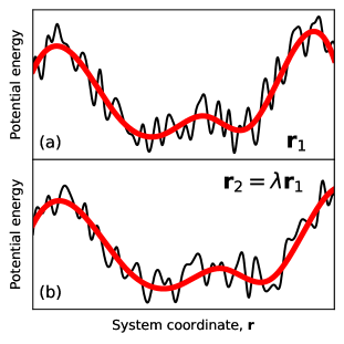
Figure 1: Coarse-graining approach for understanding hidden scale invariance. (a) The solid black line represents a conceptual sketch of the typical potential energy landscape, $U({\bf r}^{n})$, for a molecular system. The landscape exhibits two characteristic length scales: (1) fast fluctuations dominated by intramolecular vibrations and intermolecular roughness and (2) slow fluctuations representing substantial molecular rotations and translations. The slow fluctuations are indicated with a thick red line. (b) The potential energy landscape after an affine scaling of all coordinates by 10% ($\lambda=1.1$). The slow fluctuations are scale-invariant, i.e., the thick red line retains the same shape. Due to fast fluctuations, the potential energy landscape is not intrinsically scale-invariant. This paper addresses the challenge of identifying the solid red line from the black line in an atomistic description of a molecular system.

III Systematic Coarse-Graining Approaches

III.1 Need for Bottom-up Coarse-Graining

Due to the strong intramolecular interactions, the instantaneous virial and potential energy are expected to exhibit significant fluctuations at the atomistic level. In order to overcome this challenge, we propose statistical coarse-graining approaches that allow for extracting an effective one-dimensional phase diagram for these complex molecules. Our central hypothesis is that the correct coarse-graining procedure, derived from microscopic physical principles, can effectively integrate out unnecessary degrees of freedom (e.g., intramolecular vibrations) and retain only the important intermolecular motions that have strong correlations.

In this section, we introduce two separate coarse-graining methodologies, namely, coarse-graining in time and in space. Since these two approaches are derived from different motivations and underlying assumptions, we develop each coarse-graining scheme separately, apply them to the atomistic OTP, and compare their performances in Secs. IV and V, respectively. Then, combining these two coarse-graining approaches together, in Sec. VI, we assess how systematic coarse-graining approaches impart the one-dimensional phase diagram through density scaling.

III.2 Coarse-graining in time

Coarse-graining in time (or temporal coarse-graining) mitigates the fluctuations in the fully atomistic potential energy landscape by averaging the fluctuations within the characteristic time scale. Hence, this approach enables the examination of slow degrees of freedom, which can be measured, e.g., by frequency-dependent linear response functions.

The central idea underlying temporal coarse-graining is motivated by a recent striking experiment on the silicone diffusion pump oil DC704 (tetramethyltetraphenyl-trisiloxane; C₂₈H₃₂O₂Si₃) Gundermann et al. (2011). In contrast to atomic simulations, it is impractical to measure the correlation coefficient $R$ defined by the instantaneous virial-potential fluctuations from experiments. Instead, Ref. Gundermann et al., 2011 utilized the fluctuation-dissipation theorem Hansen and McDonald (1976), providing an alternative relationship to dynamic response functions, e.g., the frequency-dependent heat capacity. Generalizing the isomorph theory to frequency-dependent response functions enables scaling to be applied to the slow degrees of freedom, i.e., molecular rotational and translational motions, which freeze at the glass transition Goldstein (1969); Ediger and Harrowell (2012); Biroli and Garrahan (2013). This extension also generalizes the correlation coefficient of the isomorph theory for point particles, $R$ [Eq. (4)], to a time-dependent equivalent, $R(t)$, through experiments. In detail, experimental measurements have demonstrated that, to the first approximation, the long-time limit of $R(t)$ is related to the classic Prigogine-Defay ratio $\Pi$ by $R\simeq 1/\sqrt{\Pi}$, where $\Pi$ is the dimensionless number

$$\Pi=\frac{1}{VT}\frac{\Delta c_{p}\Delta\kappa_{T}}{(\Delta\alpha_{p})^{2}}\Biggr{|}_{T=T_{g}}\simeq\frac{1}{R^{2}},$$ (9)

which involves the jumps in the thermal expansion coefficient $\alpha_{p}$, compressibility $\kappa_{T}$, and heat capacity $c_{p}$ at the glass transition $T=T_{g}$ Prigogine and R Defay (1954); Gupta and Moynihan (1976); Takahara et al. (1999); Schmelzer and Gutzow (2006); Ellegaard et al. (2007); Pedersen et al. (2008b); Gundermann et al. (2011); Fragiadakis and Roland (2011); Casalini et al. (2011); Tropin et al. (2012); Garden et al. (2012). $\Pi$ is unity whenever the phase diagram is effectively one-dimensional.

By establishing $\Pi\simeq{1}/{R^{2}}$ [Eq. (21)] for DC704, Ref. Gundermann et al., 2011 further shed light on the strongly correlating nature of OTP in experiments. Estimating the classical Prigogine-Defay ratio for 22 glass formers from literature values, including polymers, metallic alloys, inorganic, and molecular liquids (both hydrogen-bond rich and van der Waals bonded), revealed that liquid mixtures containing OTP have $\Pi$ values near 1.2, corresponding to $R\simeq 0.9$. This indicates the existence of an effective one-dimensional phase diagram of OTP. Notably, this back-of-the-envelope estimation correctly predicts the behavior of hydrogen-bonding liquids, where glucose (C₆H₁₂O₆) and glycerol (C₃H₃O₃) have much higher ratios of $R\simeq 0.5$ each, aligning with observations from isomorph theory.

In summary, the discoveries reported in Ref. Gundermann et al., 2011 directly motivate a temporal coarse-graining approach, where the density scaling exponent $\gamma$ can be independently computed from frequency-dependent response functions. Consequently, a systematic temporal coarse-graining from first principles is expected to facilitate the understanding of isomorph theory for complex liquids currently accessible only through experiments.

III.3 Coarse-graining in space

In addition to coarse-graining in the temporal domain, one can also consider coarse-graining in space (or spatial coarse-graining) by constructing a reduced configurational representation of complex molecular systems. For OTP, this specific coarse-graining scheme is inspired by the widely adopted Lewis-Wahnström model Wahnström and Lewis (1993); Lewis and Wahnström (1993, 1994, 1994); Wahnström and Lewis (1997). This model consists of three CG sites connected via fixed bonds and interacting through a Lennard-Jones interaction to represent the OTP molecules in an ad hoc reduced form. Despite its simplicity and limitations, the Lewis-Wahnström model can reasonably simulate the chemical and physical behavior of OTP at an efficient computational cost Rinaldi et al. (2001); Lombardo et al. (2006); Pedersen et al. (2011). Notably, as expected from the fixed bond length, the Lewis-Wahnström model exhibits strong virial-potential energy correlations and obeys isomorph theory predictions Schrøder et al. (2009); Ingebrigtsen et al. (2012). However, the interaction parameters for the Lewis-Wahnstöm model are not directly parametrized from microscopic (atomistic) OTP energetics, and hence there is no clear microscopic evidence that the hidden scale invariance identified using the ad hoc three-site model is representative of atomistic OTP molecules.

Unlike the ad hoc representation, bottom-up spatial coarse-graining approaches can systematically construct a reduced model that faithfully reproduces important microscopic correlations Müller-Plathe (2002); Voth (2008); Peter and Kremer (2009); Noid (2013); Brini et al. (2013); Jin et al. (2022). Furthermore, based on fine-grained (fully atomistic) simulations, a bottom-up spatial CG method can answer the following questions. Is the Lewis-Wahnström model a microscopically consistent representation of OTP molecules? If not, to what extent does this ad hoc model accurately capture microscopic correlations at the reduced resolution? Chemical intuition suggests that bonds between linked phenyl rings in OTP should fluctuate, indicating that the underlying assumption of the Lewis-Wahnström model might be incorrect. In this regard, constructing a three-site spatial CG model using the atomistic OTP trajectory can unravel this ambiguity. By examining the stark differences between the full-atomistic level and the phenomenological CG level, introducing a systematic coarse-graining approach to complex molecules is expected to provide a microscopic understanding of density scaling relationships.

Due to the expected flexibility of intramolecular bonds in OTP, a single-site (center-of-mass) representation would be the optimal resolution for tracing out a one-dimensional phase diagram because it eliminates directional intramolecular interactions. As such, this spatial renormalization allows us to estimate the virial-potential correlation of the underlying molecule. Eventually, the single-site CG representation can provide insights into the thermodynamic scaling in the following manner: (1) how does the scaling exponent behave at the reduced resolution? By removing unnecessary degrees of freedom, one could apply ideas from the isomorph theory. (2) The renormalized interaction profile can be examined at a single-site resolution to understand the microscopically determined interaction. Based on the obtained CG interaction, we will examine whether it can be approximated as analytical interactions, e.g., IPL, to establish a systematic connection to thermodynamic scaling or effective hard sphere theory. Combined together, an overall aim is to link both the density scaling and excess entropy scaling of complex molecular liquids using this systematic spatial coarse-graining approach, as well as temporal coarse-graining.

III.4 Microscopic Reference: Atomistic Simulations

In order to perform coarse-graining in space and time, we first performed an all-atom simulation of 125 OTP molecules Greet and Turnbull (1967); Richert (2005); Takahara et al. (1999); Casalini et al. (2016); Mapes et al. (2006) using the Optimized Potentials for Liquid Simulations (OPLS) force field with charge corrections, 1.14*CM1A(-LBCC) Dodda et al. (2017). Figure 2(a) illustrates a snapshot of the OTP system modeled using this force field. The molecular shape is retained by intramolecular bonds, angles, and dihedral potential, $U_{\textrm{intra}}({\bf r}^{n})$, while the intermolecular interactions, $U_{\textrm{intra}}({\bf r}^{n})$, are described by Coulomb and Lennard-Jones interactions. The overall potential energy is represented as:

$$U({\bf r}^{n})=U_{\mathrm{intra}}({\bf r}^{n})+U_{\mathrm{inter}}({\bf r}^{n}).$$ (10)

where

$$U_{\mathrm{intra}}({\bf r}^{n}) =\sum_{\mathrm{bonds}}K_{r}(r_{ij}-r_{\mathrm{eq}})^{2}+\sum_{\mathrm{angles}}K_{\theta}(\theta_{ijk}-\theta_{\mathrm{eq}})^{2}$$

$$+\sum_{\mathrm{dihedrals}}V(\phi_{ijkl})$$ (11)

with $V(\phi_{ijkl})=\sum_{n=1}^{3}V_{n}\cos(n\phi_{ijkl}+f_{n})/2$, and

$$U_{\mathrm{inter}}({\bf r}^{n})=\sum_{i>j}\frac{q_{i}q_{j}e^{2}}{r_{ij}}+\frac{A_{ij}}{r_{ij}^{12}}-\frac{C_{ij}}{r_{ij}^{6}}$$ (12)

with $r_{ij}=|{\bf r}_{j}-{\bf r}_{i}|$ as a pair distance. The parameters ($K_{r}$, $r_{\mathrm{eq}}$, $K_{\theta}$, $\theta_{\mathrm{eq}}$, $V_{n}$, $f_{n}$, $q_{i}$, $A_{ij}$ and $C_{ij}$) are chosen according to Ref. Dodda et al., 2017.

In order to investigate density scaling, various thermodynamic state points of OTP were investigated at the atomistic level using Eqs. (10)-(12). The explored state points are depicted in Fig. 2(b), where the temperature ranges from 380 to 700 K and the (mass) density from 0.878 to 1.115 g/cm³ (corresponding to the box lengths from 37.899 to 35 Å), falling between the experimental conditions studied for OTP. At each state point, constant temperature molecular dynamics simulations Grønbech-Jensen and Farago (2014); Grønbech-Jensen et al. (2014) were carried out for durations between 70 and 400 ns using the LAMMPS software package Thompson et al. (2022).

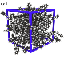
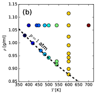
Figure 2: Microscopic MD simulation details of the OTP system. (a) Snapshot from an atomistic simulation of 125 OTP molecules. The blue lines indicate the periodic boundaries of the simulation box. (b) Thermodynamic state points investigated in this work. The dashed line indicates state points of ambient pressure ($p=1$ atm).

IV Coarse-graining in time

IV.1 Theory of Temporal Coarse-Graining

The central goal of coarse-graining in time is to average out fast degrees of freedom while retaining the slow degrees of freedom. Hereafter, we assume the system is at a sufficiently low temperature, where intramolecular degrees of freedom, such as bond vibrations, are considerably faster than molecular motions, e.g., translational motions. We consider temporal averaging characterized by a time scale, $\tau$, or the inverse angular frequency, $\omega^{-1}$, chosen to be faster than the intermolecular dynamics but slower than intramolecular motions. In general, the optimal $\tau$ and $\omega$ depend on the specific observable from OTP intended to be CG in time. In this section, we will introduce several temporal coarse-graining methodologies and show that these different approaches capture nearly the same strong correlation nature for OTP.

IV.2 Time-Averaging Approach

Arguably, the most straightforward method for implementing temporal coarse-graining would be to perform a time average of the potential energy $U(t)$ and the virial $W(t)$. This time-averaging approach is motivated by a typical experimental setting, where measuring fluctuations using a probe often encounters an effective “low-pass” filter. This essentially corresponds to the temporal CG quantity $\bar{f}(t;\tau)$, which can be expressed as a convolution

$$\bar{f}(t;\tau) = \int_{-\infty}^{\infty}f(t^{\prime})w(t-t^{\prime};\tau)dt^{\prime},$$ (13)

where $w(t;\tau)$ is a kernel with the property $\int_{-\infty}^{\infty}w(t;\tau)dt=1$ (not to be confused with the angular frequency $\omega$) that describes how the averaging is distributed in time. It is worth noting that $\bar{f}$ is associated with slow fluctuations if the $w$ function has a significant width, usually quantified by a large value of the $\tau$ parameter. The quantity $\bar{f}(t;\tau)$ is relevant to experimental measurements, where $f(t)$ might not be readily available. We implemented a discrete analog of Eq. (13) using the SciPy Python package Virtanen et al. (2020).

Figure 3: Schematic description of the proposed temporal coarse-graining: (a) Fully atomistic simulation trajectories give energetics with frequent fluctuations (green lines) due to intramolecular interactions and motions (green arrows). (b) By temporal coarse-graining the energetics over the characteristic time $\tau$, one can focus on the slow fluctuations (black lines) due to the intermolecular interactions.

The $w$ is typically an exponential decay, a Gaussian function, or the Hann function. In this work, we adopt the “boxcar” average, where $\bar{f}(t,\tau)$ is computed by averaging values from $f(t)$ to $f(t+\tau)$ with equal weight. The temporal coarse-graining is then achieved by using a rectangular window as the $w$ function, defined as

$$w(t;\tau)=\begin{cases}0&\text{for }t<0,\\ 1/\tau&\text{for }0\leq t\leq t+\tau,\\ 0\quad&\text{for }t>t+\tau.\\ \end{cases}$$ (14)

As $w(t;\tau)\rightarrow\delta(t)$ for $\tau\rightarrow 0$, the direct signal, $f(t)$, is recovered in the limit $\tau\to 0$.

Figure 4(a) illustrates the boxcar average of potential energy fluctuations with averaging lengths ranging from $\tau=1$ ps to $\tau=10$ ns at $T=380$ K and $\rho=1.029$ g/ml, corresponding to ambient pressure. As expected, the fluctuations decrease as $\tau$ increases. Figure 4(b) displays the time-averaged potential energy, the average of the intramolecular contribution, and of the intermolecular contribution with $\tau=1$ ns, representing slow fluctuations. Notably, using $\tau=1$ ns, the kinetic energy fluctuations have diminished, whereas the fluctuations of intermolecular energy remain significant. The data show that upon temporal coarse-graining, the slow fluctuations are representative of the intermolecular contributions.

In order to systematically investigate the impact of $\tau$, Fig. 4(c) presents the standard deviation as a function of $\tau$, revealing that slow energetic fluctuations are observed when the width of the average is on the order of a nanosecond for the investigated state point. We have noticed that for some state points, separating fast and slow fluctuations is not possible, especially when the structural relaxation time is significantly faster than one nanosecond. Moreover, in scenarios of low temperatures or high densities, obtaining good statistics for slow fluctuations can be challenging as the dynamics become sluggish. In this study, we find that a one-nanosecond relaxation time is an appropriate characteristic time for temporal coarse-graining in the context of OTP. Table 1 lists additional $\tau$ values that are systematically determined across various state points through the aforementioned coarse-graining process.

Next, we investigate whether the CG energy landscape exhibits strong correlations and eventually scale invariance, as depicted in Fig. 1. Drawing inspiration from the formalism of the isomorph theory for point particles, we expect strong correlations in the slow fluctuations between the potential energy and the virial: While the instantaneous fluctuations of potential energy and virial themselves are uncorrelated [Fig. 5(a)], the slow fluctuation are correlated [Fig. 5(b)]. Therefore, as an analogy to the isomorph theory, the Pearson correlation coefficient,

$$R_{\bar{U}\bar{W}}(\tau)=\frac{\langle\Delta\bar{W}\Delta\bar{U}\rangle}{\sqrt{\langle(\Delta\bar{W})^{2}\rangle\langle(\Delta\bar{U})^{2}\rangle}}$$ (15)

should be close to unity. As depicted in Fig. 6(a), $R_{\bar{U}\bar{W}}(\tau)$ approaches 0.86 for $\tau>$ 1 ns, indicating a strongly correlating nature. This also suggests that the slowly fluctuating part of the potential energy landscape is scale-invariant, aligning with the illustration in Fig. 1. Building upon this observation of strong correlations, we proceed to compute the density scaling exponent from temporal coarse-graining using

$$\gamma_{\bar{U}\bar{W}}(\tau)=\frac{\langle\Delta\bar{W}\Delta\bar{U}\rangle}{\langle(\Delta\bar{U})^{2}\rangle}.$$ (16)

As demonstrated in Fig. 6, the exponent converges to 6.3(3). Extending this approach to other state points with similar structural relaxation times, the averaged estimates for scaling exponents reported in Table 1 consistently yield $\gamma$ values of 6.3 within statistical uncertainty.

In summary, we demonstrated that by directly performing time averaging of fluctuating atomistic virial and potential energies, we obtained an average value of $\gamma=6.3$ for atomistic OTP, confirming its strongly correlating nature, which was not previously feasible. Before examining whether this $\gamma$ value correctly encodes the one-dimensional phase diagram of OTP, we will validate if our time-averaging approach represents the correct temporal CG characteristic of OTP in the remainder of this section, using alternative approaches inspired by experimental observations.

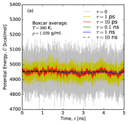
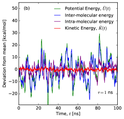
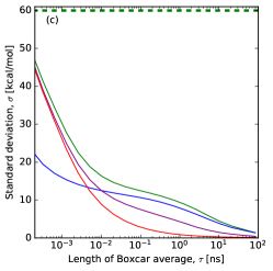
Figure 4: Temporal coarse-graining by the time-averaging approach. (a) Boxcar average of the potential energy, $\bar{U}(t;\tau)$, in a simulation of 125 OTP molecules at $T=380$ K and $\rho=1.029$ g/ml (1 atm) for different choices of the characteristic time scale, $\tau$ (see legend). For clarity, only 5 ns of the 468 ns simulation is shown. (b) Various time-averaged observables using $\tau=1$ ns, including the time-averaged potential energy (green); intermolecular (blue) and intramolecular (purple) energies decomposed using Eq. 10; and kinetic energy (red). (c) Standard deviations of the time-averaged energetics from panel (b) of the potential, intermolecular, intramolecular, and kinetic energies, respectively.

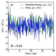
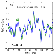
Figure 5: $WU$ fluctuations from time-averaged CG OTP. (a) Normalized times series, $(y(t)-\langle y\rangle)/\sigma_{y}$ (where $\sigma_{y}$ is the standard deviation), of potential energy (green) and viral (blue). The correlation is weak, quantified by the Pearson correlation coefficient $R=0.01$. (b) Boxcar averaged energy (green) and virial (blue) fluctuations. The correlation is strong, quantified by $R=0.86$. Note that the time-axis on this panel is in units of nanoseconds, while it is in picoseconds in the first panel.

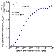
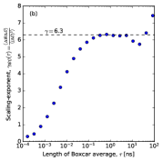
Figure 6: Correlation coefficients from time-averaged CG OTP. (a) The Pearson correlation coefficient of the boxcar averaged potential energy ($\bar{U}$) and virial ($\bar{W}$), as a function of the length of the boxcar average, $R_{\bar{W}\bar{U}}(\tau)=\frac{\langle\Delta\bar{W}\Delta\bar{U}\rangle}{\sqrt{\langle(\Delta\bar{W})^{2}\rangle\langle(\Delta\bar{U})^{2}\rangle}}$. Strong correlations of the slow $\bar{U}$ and $\bar{W}$ fluctuations are evident as $R\to 0.86$ for $\tau\to\tau_{\alpha}$ (black dashed line). (b) Density scaling exponent ($\gamma$) estimated from $\bar{U}$ and virial $\bar{W}$. We find that $\gamma\to 6.3$ for $\tau\to\tau_{\alpha}$ (black dashed line).

Table 1: State points where the density scaling exponent could be accurately determined from the slow $\bar{W}(t)$-$\bar{U}(t)$ fluctuations using a boxcar average, compare Fig. 6. The structural relaxation time $\tau_{\alpha}$ is estimated as shown in Fig. 7(a).

$T$ [K]	$\rho$ [g/mL]	$\tau_{\alpha}$ [ns]	$\gamma$
$360$	$1.045$	$1.0$	$6.1$
$380$	$1.029$	$0.5$	$6.3$
$400$	$1.060$	$2.0$	$6.0$
$400$	$1.014$	$0.1$	$6.2$
$500$	$1.096$	$1.0$	$7.0$
$500$	$1.078$	$0.4$	$6.3$

IV.3 Time Correlation Function Approach

As we are interested in the time series of fluctuations, an alternative approach to performing temporal coarse-graining can be derived from the time correlation formalism. The time correlation function between two signals $f$ and $g$ with a lag time $\tau$ is defined as

$$C_{fg}(\tau)=\overline{f(\tau)g(0)}=\lim_{T_{0}\rightarrow\infty}\frac{1}{T_{0}}\int_{0}^{T_{0}}f(t+\tau)g(t)dt.$$ (17)

Efficient computation of Eq. (17) is possible through the cross-correlation theorem combined with the Fast Fourier Transform (FFT) algorithm, as described in Ref. Press et al., 2007. To briefly outline the standard procedure we followed, let $\mathcal{F}[y(t)]=\int_{-\infty}^{\infty}y(t)\exp(-i\omega t)dt$ be the Fourier transform, and let $\mathcal{F}^{-1}[Y(\omega)]=\int_{-\infty}^{\infty}Y(\omega)\exp(i\omega t)d\omega$ be the inverse Fourier transform. Then, the time correlation function $C_{fg}$ can be expressed through the inverse Fourier transform of the convolution in the frequency domain:

$$C_{fg}(\tau)=\mathcal{F}^{-1}[F^{*}(\omega)G(\omega)],$$ (18)

where $F(\omega)=\mathcal{F}[f(t)]$, $G(\omega)=\mathcal{F}[g(t)]$, and $(\ldots)^{*}$ represents the complex conjugate. From its definition, Eq. (17) represents slow fluctuations as $\tau$ increases.

In order to assess the CG virial potential-energy correlation using the time correlation formalism, Fig. 7(a) illustrates the time correlation function of the potential energy with itself over time, $C_{UU}(t)$—the auto-correlation function, at the same thermodynamic state point as investigated in the previous subsection using time-averaging (Figs. 4–6): $380$ K; $1.029$ g/ml; 1 atm. The auto-correlation function depicted in Fig. 7(a) demonstrates the multi-step relaxation nature of potential energy surfaces. As the terminal relaxation is associated with important molecular translations and rotations, we estimated the structural relaxation time underlying this terminal relaxation by fitting to a stretched exponential: $A\cdot\exp\left[-(t/\tau_{\alpha})^{\beta}\right]$. At this specific state point, the structural relaxation time was determined to be $\tau_{\alpha}=0.5$ ns, which is within the same order of magnitude as the time scale obtained from the time-averaging method [cf. Fig. 4(c) and Fig. 7(a)].

As we apply the time correlation formalism to other fluctuating quantities, a strong correlation of the slow energy-virial fluctuations becomes evident. In Fig. 7(b), we observe that the long-time (slow) relaxation behavior of $C_{UU}(t)$, $C_{WW}(t),$ and $C_{UW}(t)$ coincide near the terminal relaxation time. This feature greatly suggests a strong correlation between the virial and the potential energy at this characteristic time. Based on these findings, we computed the scaling exponent estimated from the time correlation function [Fig. 7(c)]

$$\gamma_{C}(t)=\frac{C_{UW}(t)}{C_{UU}(t)},$$ (19)

which provides a value consistent with that of the time-averaging approach [Fig. 6(b)]: $\gamma=6.3$, highlighting the validity of the two temporal CG approaches.

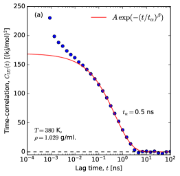
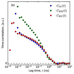
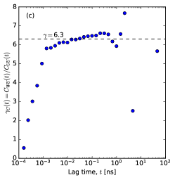
Figure 7: Temporal coarse-graining by the time correlation function approach. (a) Auto-correlation functions of the potential energy fluctuations, $C_{UU}(t)$. The long-time decorrelation of energy fluctuations is used to estimate the structural relaxation time of the system to $\tau_{\alpha}=0.5$ ns by fitting to a stretched exponential $A\cdot\exp\left[{-(t/\tau_{\alpha})^{\beta}}\right]$ (red line), where $A=170$ (kJ/mol)² and $\beta=0.62$. (b) Comparison of the time correlation functions $C_{UU}(t)$, $C_{WW}(t)$, and $C_{UW}(t)$. The vertical axis has been scaled so that long-time relaxation overlaps with the expected correlations from slow fluctuations. (c) The scaling exponent estimated from the time correlation functions, see Eq. (19), is consistent with the results of Fig. 6.

IV.4 Frequency-Dependent Response Approach

Our final temporal CG approach is directly inspired by studies on the frequency-dependent Prigogine-Defay ratio aimed at understanding density scaling Ellegaard et al. (2007); Pedersen et al. (2008b); Pedersen (2009); Gundermann et al. (2011). This concept can be formally derived from the fluctuation-dissipation theorem, which links the power spectrum of fluctuations in equilibrium to frequency-dependent linear response functions. Generally, a frequency-dependent response function related to the variables $f$ and $g$ can be computed as a Fourier-Laplace transform

$$\mu_{fg}(\omega)=\int_{0}^{\infty}\dot{C}_{fg}(t)\exp(-i\omega t)dt,$$ (20)

in which $\dot{C}_{fg}(t)=\frac{d}{dt}C_{fg}(t)$. Since $\dot{C}_{fg}$ approaches zero when $t\rightarrow 0$, the integral in Eq. (20) can be treated as a conventional Fourier transform when $\dot{C}_{fg}(t)$ is prescribed to be zero at negative times. Consequently, this quantity can be efficiently computed using the FFT algorithm. For example, the frequency-dependent heat capacity can be estimated from $c_{V}(\omega)=-\mu_{UU}(\omega)/k_{B}T^{2}$ Nielsen and Dyre (1996).

Having established the relationship between the frequency-dependent response function and the power spectrum of fluctuations, we now evaluate the correlation between the virial and the potential energy fluctuations. At low angular frequencies ($\omega$), corresponding to long time scales, this can be done by assessing $\mu_{UU}(\omega)$, $\mu_{WU}(\omega)$, and $\mu_{WW}(\omega)$, as depicted in Fig. 8(a). From these frequency-dependent response functions, the generalized correlation coefficient, which is also frequency-dependent, between two signals can be defined in a manner analogous to the frequency-dependent Prigogine-Defay ratio Ellegaard et al. (2007); Pedersen et al. (2008b); Pedersen (2009); Gundermann et al. (2011):

$$R_{\mu}(\omega) \equiv \frac{\mathfrak{I}\mu_{UW}(\omega)}{\sqrt{\mathfrak{I}\mu_{WW}(\omega)\mathfrak{I}\mu_{UU}(\omega)}}.$$ (21)

In Eq. (21), $\mathfrak{I}(\ldots)$ denotes the imaginary part of the complex response functions. In practice, we note that $R_{\mu}(\omega)$ is rather noisy, yet it confirms the existence of strong virial-potential energy fluctuations. From Eq. (21), the corresponding frequency-dependent scaling exponent can be defined as

$$\gamma(\omega)=\frac{\mathfrak{I}\mu_{WU}(\omega)}{\mathfrak{I}\mu_{UU}(\omega)},$$ (22)

which can still be estimated from the noisy response functions. Figure 8(b) further confirms the validity of our approach, consistently yielding a $\gamma=6.3$ value as with the two previous approaches.

IV.5 Summary

We have introduced three methods for coarse-graining the fast intramolecular degrees of freedom in OTP molecules over a temporal domain. By effectively retaining the slow degrees of freedom through temporal coarse-graining, we have shown that this temporal CG approach allows for uncovering strong correlations between the virial and potential energy of OTP, which are challenging to assess at a fully atomistic resolution. In particular, our temporal coarse-graining approaches include (1) direct time-averaging of fluctuating virial and potential energy, (2) indirect coarse-graining of the time correlation formalism in conjunction with the Fourier transformation, and (3) utilization of a frequency-dependent response to coarse-grain the power spectrum of fluctuations via the fluctuation-dissipation theorem.

We implemented three different temporal CG approaches for OTP across various temperature and density conditions. These three distinct approaches all remarkably provide a consistent scaling exponent of $\gamma=6.3$ at various thermodynamic state points. This agreement indicates that, while the approaches are derived differently, the underlying physical picture of the strong correlation in OTP is invariant. Nevertheless, among the different approaches, we note that the time-averaging method could be easily extended to other complex molecules as it provides better statistics and is relatively easy to implement compared to the other two approaches. Altogether, temporal coarse-graining reveals a hidden scale invariance from the slow fluctuations in the OTP energy landscape [e.g., Fig. 5(b)], demonstrating that $U({\bf r}^{n})$ in OTP resembles the landscape hypothesized in Fig. 1.

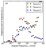
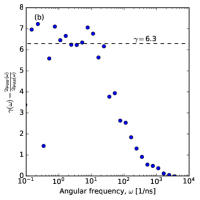
Figure 8: Temporal coarse-graining by the frequency-dependent linear response function approach. (a) Imaginary parts of frequency-dependent response functions. (b) The frequency-dependent scaling exponent.

V Coarse-Graining in Space

V.1 Theory of Spatial Coarse-Graining

While coarse-graining in time entails convoluting the observables over time, coarse-graining in space aims to simplify the target molecular system itself Müller-Plathe (2002); Voth (2008); Peter and Kremer (2009); Noid (2013); Brini et al. (2013); Jin et al. (2022). In the case of OTP, the primary objective is to design a single-site CG model free of intramolecular interactions. The desired spatial CG model should accurately capture the effective correlations of atomistic OTP molecules at the center-of-mass level, as depicted in Fig. 9(a). Bottom-up (spatial) coarse-graining approaches are, therefore, the optimal strategy for performing coarse-graining in space, as the central aim of bottom-up coarse-graining is to faithfully recapitulate the microscopic (atomistic) correlations at the spatial CG level Noid (2013); Jin et al. (2022).

Consider a spatial coarse-graining mapping operator, denoted as $M_{\mathbf{R}}^{N}$, which transforms the fine-grained (atomistic) configurations $\mathbf{r}^{n}$ into the CG configurations $\mathbf{R}^{N}$, i.e., $M_{\mathbf{R}}^{N}:\mathbf{r}^{n}\rightarrow\mathbf{R}^{N}$. The CG model correctly approximates the fine-grained (FG) reference when the following consistency condition regarding the equilibrium probability distributions of the FG and CG variables in phase space is satisfied Noid et al. (2008a, b):

$$p_{\mathrm{CG}}({\bf R}^{N})=\int d\mathbf{r}^{n}\delta\left(M_{\mathbf{R}}^{N}(\mathbf{r}^{n})-\mathbf{R}^{N})\right)p_{\mathrm{FG}}(\mathbf{r}^{n}),$$ (23)

where the overall delta function enforces that the mapped FG configurations are matched to the CG configurations, and it is understood as a product of delta functions for each CG particle $I$, i.e., $\delta\left(M_{\mathbf{R}}^{N}(\mathbf{r}^{n})-\mathbf{R}^{N})\right)=\prod_{I}^{N}\left(\delta\left(M_{I}(\mathbf{r}^{n})-\mathbf{R}_{I}\right)\right)$. From the thermodynamic consistency relationship for configurational variables [Eq. (23)], the effective CG interaction $U_{\mathrm{CG}}$ can be derived as

$$U_{\mathrm{CG}}= -k_{B}T\ln\int d\mathbf{r}^{n}\delta\left(M_{\mathbf{R}}^{N}(\mathbf{r}^{n})-\mathbf{R}^{N}\right)$$

$$\times\exp\left(-\frac{u_{\mathrm{FG}}(\mathbf{r}^{n})}{k_{B}T}\right)+\mathrm{(constant)},$$ (24)

where $u_{\mathrm{FG}}(\mathbf{r}^{n})$ represents the FG interaction potential. It is worth noting that $U_{\mathrm{CG}}$ in Eq. (V.1) takes the form of the many-body potential of mean force (PMF) in terms of CG variables Noid et al. (2008a, b). Therefore, $U_{\mathrm{CG}}(\mathbf{R}^{N})$ can be interpreted as a free energy-like quantity, and in general it will vary with the thermodynamic state point. This state point-dependent nature of the CG interactions is referred to as the transferability issue in CG modeling Dunn et al. (2016); Jin et al. (2019, 2020).

While Eq. (V.1) is formally exact such that it yields a thermodynamically consistent CG model, the practical determination of $U_{\mathrm{CG}}$ through the many-dimensional integration is highly prohibitive in practice. Various optimization schemes have been developed to overcome this challenge. In this work, we employ a multiscale coarse-graining (MS-CG) methodology Noid et al. (2008a, b), which utilizes force-matching to determine $U_{\mathrm{CG}}$ Lu et al. (2010). This is achieved by variationally minimizing the force residual $\chi^{2}[\phi]$, which is the force difference between the microscopic reference force at the CG level, $\mathbf{f}_{I}(\mathbf{r}^{n})$, and the unknown CG force, $\mathbf{F}_{I}(M_{\mathbf{R}}^{N}(\mathbf{r}^{n});\phi)$, defined using the CG force field parameter $\phi$:

$$\chi^{2}[\phi]=\frac{1}{3N}\langle\sum_{I=1}^{N}|\mathbf{F}_{I}(M_{\mathbf{R}}^{N}(\mathbf{r}^{n});\phi)-\mathbf{f}_{I}(\mathbf{r}^{n})|^{2}\rangle.$$ (25)

Therefore, $\phi$ can be determined by minimizing Eq. (25). Noid et al. further demonstrated that the least-squares solution to Eq. (25) satisfies the consistency relationship given in Eq. (23) Noid et al. (2008a). This thermodynamically consistent CG model also captures important structural correlations from the atomistic reference: Ref. Noid et al., 2007 established that the force-matching equation [Eq. (25)] employing two-body basis sets is a discretized representation of the Yvon-Born-Green theory in liquid physics Hansen and McDonald (1976). This finding suggests that the MS-CG model can effectively capture up to three-body correlations using two-body basis sets, distinguishing it from other bottom-up methodologies. Therefore, the MS-CG method stands as a robust choice for constructing a CG model of OTP with high structural accuracy.

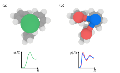
Figure 9: Schematic of the proposed spatial coarse-graining with two different mapping schemes and the corresponding radial distribution functions : (a) Single-site CG model at the center-of-mass level. The single-site resolution integrates the intramolecular degrees of freedom and thus is suitable to investigate hidden scale invariance. (b) Three-site CG model. This resolution is adopted by the ad hoc Lewis-Wahnström model but lacks the link to microscopic physics.

V.2 Spatial CG Model of OTP

V.2.1 Settings and computational details

The construction of the spatially CG model for OTP proceeded as follows. From atomistic MD trajectories, we mapped OTP molecules to their center-of-masses. The mapping operator $M_{\mathbf{R}}^{N}$ maps the configuration of each molecule to its center-of-mass with the accumulated force $\mathbf{f}_{I}(\mathbf{r}^{n})=\sum_{i\in\mathcal{I}_{I}}\mathbf{f}_{i}^{\mathrm{FG}}$, where $\mathbf{f}_{i}^{\mathrm{FG}}$ denotes the microscopic force acting on atom $i$ within the set of atoms $\mathcal{I}_{I}$ mapped to the CG site $I$.

From the mapped atomistic trajectory, the effective CG interaction of OTP was then determined by utilizing Eq. (25) Peng et al. (2023). In practice, the CG force field, as seen in Eq. (25), is expressed using pairwise basis sets $\phi_{2}(R_{IJ})$ for the CG pair $I$ and $J$, resulting in

$$\mathbf{F}_{I}(M_{\mathbf{R}}^{N}(\mathbf{r}^{n});\phi_{2})=\sum_{J\neq I}\phi_{2}(R_{IJ})\hat{e}_{IJ},$$ (26)

where $\hat{e}_{IJ}$ denotes the unit vector of $\mathbf{R}_{IJ}$. To capture the intricate profile of molecular interactions, we introduced the B-spline function $\{u_{k}\}$ with coefficients $c_{k}$ to define the pairwise basis, i.e., $\phi_{2}(R_{IJ})=\sum_{k}c_{k}u_{k}(R_{IJ})$. The effective CG force field can then be expressed as $\mathbf{F}_{I}(M_{\mathbf{R}}^{N}(\mathbf{r}^{n});\phi_{2})=\sum_{J\neq I}\sum_{k}c_{k}u_{k}(R_{IJ})\hat{e}_{IJ}$, and Eq. (25) reduces to an overdetermined system of linear equations Press (2007) of the following form:

$$\mathbf{F\phi}_{2}=\mathbf{f}.$$ (27)

Here, the matrix $\mathbf{F}$ represents the CG forces expressed through the overall CG configurations and basis functions $\mathbf{\phi}_{2}$, while $\mathbf{f}$ denotes the mapped atomistic forces at the CG level. For a more in-depth discussion of the interpolation scheme and implementation details, readers are referred to Ref. Lu et al., 2010. Utilizing B-splines in the parametrization allows for capturing complex interaction profiles that cannot be fully resolved using analytical interaction. However, this introduces a numerical challenge when estimating the derivatives of interactions. This drawback will be discussed in more detail in Sec. V.4.1, when directly estimating the density scaling exponent $\gamma$ from the CG models.

V.2.2 Parametrized Interaction

The effective pairwise CG interactions of OTP were parametrized by solving Eq. (27) across the thermodynamic state points investigated in Sec. III.4 spanning temperatures from 380 to 700 K and densities from 0.878 to 1.115 g/cm³. Based on the previously reported characteristics of OTP interactions, we selected a spline resolution of 0.2 Å and sampled the interaction up to a cutoff of 10.0 Å.

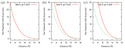
Figure 10: Parametrized pair interactions of the single-site CG OTP at three state points: (a) 380 K, 1.029 g/ml, (b) 600 K, 1.025 g/ml, (c) 700 K, 1.069 g/ml. Due to the free energy nature of CG interactions, the OTP CG interactions vary with temperature and density, as evident when compared to panel (a), which is represented by green dots in panels (b) and (c).

In Fig. 10, the parametrized CG interactions for three different temperature and density conditions out of 23 state points are illustrated. For clarity, the CG interactions at the remaining state points are provided in Appendix A. The CG OTP interactions are consistently repulsive, regardless of the thermodynamic conditions. Generally, $U(R)$ is always positive and appears to decay around 14–16 Å with subtle variations in positions and slopes. These changes arise from the free energy nature of bottom-up CG interactions, as expressed in Eq. (V.1); $U_{\textrm{CG}}$ varies with temperature, pressure, and other thermodynamic state variables, as extensively demonstrated in liquid systems Allen and Rutledge (2009); Lu and Voth (2011); Hsu et al. (2015); Jin et al. (2019, 2020).

The purely repulsive profile may signify the strongly correlating nature of CG OTP. Furthermore, the CG OTP interactions may be approximated as interactions following an IPL form. Given that IPL interactions strictly follow isomorph theory and adhere to density scaling, this avenue could be a viable approach for assessing the isomorph nature of atomistic OTP. However, for this mapping to be effective, a comprehensive and quantitative assessment of CG interactions is necessary. Before delving into the density scaling of CG OTP, it is imperative to validate whether the resulting CG interactions can faithfully reproduce the important structural correlations observed at the microscopic level.

V.2.3 Validating CG Models: Structural Correlations

To gauge the performance of the CG models of OTP, we perform CG simulations utilizing the obtained interactions and compute the radial distribution function (RDF) of the center-of-mass configurations, i.e., the intermolecular RDF. For each thermodynamic state point, we constructed a separate CG system and conducted constant NVT dynamics for 5 ns, employing the same thermostats as in the atomistic simulation. Using the last snapshot from the atomistic simulation, we performed the center-of-mass coarse-graining to generate the initial configuration for CG runs. The CG RDFs are then calculated from the CG simulations (Fig. 11). Likewise, the CG RDFs at other thermodynamic state points are presented in Appendix A (Fig. 17).

In spite of the purely repulsive nature of the interaction profile, our observation indicates that the CG simulation can faithfully reproduce the atomistic RDF across all thermodynamic state points studied. Even though high-resolution structural characteristics are inevitably lost at this level of coarse-graining, we note that the RDFs exhibit subtle structuring near 4-6 Å and the first peak around 8 Å. Notably, the CG models can capture the general shape and structure of the RDF within a 0.1 value range. Despite the approximations introduced, such as pairwise decomposability, we conclude that the CG model captures the essential structural correlations of OTPs.

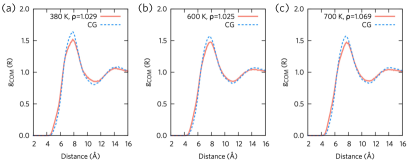
Figure 11: Center-of-mass pair correlation functions $g_{\mathrm{COM}}(R)$ for atomistic (red lines) and the single-site CG (blue dots) simulations of OTP at three state points: (a) 380 K, 1.029 g/ml, (b) 600 K, 1.025 g/ml, (c) 700 K, 1.069 g/ml. Over a wide range of temperatures ($\Delta T=320$ K) and densities ($\Delta V=11561\mbox{\AA}^{3}$), the spatial CG approach reproduces structural correlations.

V.3 Bottom-up Connection to ad hoc Lewis-Wahnström Model

V.3.1 Three-site CG Model

While Fig. 11 illustrates that the purely repulsive CG interaction can correctly capture structural correlations at the center-of-mass level, the purely positive (repulsive) nature of this interaction may seem counter-intuitive at first glance. This is because the commonly adopted potential for the three-site Lewis-Wahnström model comprises nonbonded interactions of Lennard-Jones form. Hence, understanding how coarse-graining three-site Lennard-Jones chain to the single-site resolution becomes purely repulsive, or vice versa, is not straightforward. This mismatch perhaps implies that the Lewis-Wahnström model might not be the correct representation of microscopic OTP molecules at the three-site resolution. To note, a systematic assessment of the fidelity of the Lewis-Wahnström model in comparison with the microscopic reference is lacking in the literature. Therefore, we next performed bottom-up coarse-graining of the atomistic OTP to the three-site resolution according to the schematic designed in Fig. 9(b) by mapping each benzene ring to the CG site.

The original OTP model by Lewis and Wahnström represents the OTP molecule as three particles interacting through a Lennard-Jones potential with $\varepsilon/k_{B}=600$ K (i.e., 1.1923 kcal/mol) and $\sigma=4.83$ Å. The intramolecular interactions are constrained with a fixed bond length of $\sigma$ and a fixed angle of $75^{\circ}$. Although these fixed intramolecular bonds and angles allow for exhibiting strong potential-virial correlations, this ad hoc description does not align with chemical details and hence may miss microscopic details; the correct atomistic description of chemical bonds between benzene rings should be flexible. Additionally, in the Lewis-Wahnström model, all three sites are considered equivalent with identical Lennard-Jones interactions, but two CG particles at the end (tail) should differ from the CG particle in the middle (center), as the center CG site has one less hydrogen atom. This difference implies that tail-tail, center-center, and tail-center pairs should have distinct interaction profiles, at least in principle.

To validate this ad hoc description and gain deeper insight into the energetics at the single-site level, we propose a three-site CG model of OTP constructed from the first condition presented in Fig. 10 at the following thermodynamic state points: $T=380$ K, $\rho=1.029$ g/ml. Without loss of generality, one can readily apply the same protocol to other thermodynamic state points illustrated in Fig. 2 that exhibit similar energetics. In order to account for flexible topology, we also introduce fourth-order B-splines for the bonded interactions with a resolution of $0.20$ Å. From manually mapped three-site trajectories of atomistic simulations, we observed that the bond length fluctuates from 4.09 to 4.65 Å, supporting the initial hypothesis. Finally, the three-site spatial CG model was constructed by applying force-matching [Eq. (25)] with bonded interactions.

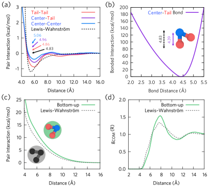
Figure 12: Assessing the ad hoc Lewis-Wahnström model (dotted lines) using the bottom-up three-site spatial CG model (solid lines). (a) Effective pair interactions. Bottom-up CG interactions exhibit a heterogeneous nature between tail and center CG sites with numbers indicating the zero interaction distance $R_{0}$, where $U(R_{0})=0$. (b) Parametrized bond interactions from atomistic statistics, exhibiting a fluctuating nature, unlike the Lewis-Wahnström model with 9.1% shorter bond length. Despite these differences, (c) and (d) show that the purely repulsive interactions and pair correlations at the single-site level from the Lewis-Wahnström model (black dots) are qualitatively consistent with the bottom-up one-site CG models (green lines), respectively.

V.3.2 Results

For the non-bonded interactions, the tail and center CG sites depicted in Fig. 12(a) exhibit slightly different energetics but similar overall interaction profiles. Thus, we observe that the ad hoc Lewis-Wahnström model provides a good approximation of the site-site CG interactions. The qualitative agreement of the Lewis-Wahnström model is attributed to its ability to capture short-range attractions. Yet, in a quantitative sense, the ad hoc interaction is closest to the tail-tail interaction among the three pair interactions, with a difference of up to 0.2 kcal/mol. Due to the heterogeneity of CG sites, the center CG site exhibits less strong attraction, which is missing in the ad hoc treatment. Additionally, the ad hoc model is characterized by a single Lennard-Jones interaction with a long-range decay scaling as $R^{-6}$, whereas the bottom-up derived interactions show slightly more complex decaying profiles with additional long-range valleys.

In Fig. 12(b), in alignment with atomistic statistics, the parametrized CG bonded interaction exhibits a flexible, harmonic-like profile with a minimum of 4.39 Å, which is shorter than the Lewis-Wahnström value of $\sigma=4.83$ Å. From this bond length, the mismatched bond interaction is approximately 30 kcal/mol, which is about 40 $k_{B}T$, indicating inaccuracies in overall energetics during computer simulations. Taken together, Figs. 12(a) and (b) suggest that the Lewis-Wahnström model can serve as a qualitative approximation of the accurate bottom-up CG model. Then, the next step would be to examine whether the purely repulsive interaction profile at the single-site resolution is consistent with the description given by the Lewis-Wahnström model.

In order to construct a single-site representation from the Lewis-Wahnström model, we first generated the Lewis-Wahnström system under the same temperature and density conditions (380 K and 1.029 g/ml, respectively). After placing 125 Lewis-Wahnström molecules with correct bonding constraints, energy minimization using the stochastic descent algorithm was performed to eliminate artificial strains applied to the system. Then, we conducted the Lewis-Wahnström simulation while fixing the bonds and angles. Finally, from the propagated CG trajectories, three-site OTP models were mapped into a center-of-mass CG model, and then we used the same protocol described above to determine the effective Lewis-Wahnström interaction at the single-site resolution.

Figure 12 compares the obtained single-site ad hoc interaction with the spatial CG interaction. Notably, we still observe a purely repulsive interaction profile, even from the one constructed from the Lewis-Wahnström model. In other words, for both analytic and phenomenological models, the coarse-graining of three Lennard-Jones sites at the fixed topology can cancel out short-range attractions at the center-of-mass level. This leads to the important conclusion that the purely repulsive nature depicted in Fig. 10 is not merely a numerical artifact but is indeed consistent with the phenomenological model. This conclusion is further substantiated by the additional analysis presented in Fig. 12(d) in terms of center-of-mass RDF. The single-site CG RDF of the Lewis-Wahnström model shows a trend consistent with the bottom-up reference constructed from atomistic simulations, where the slight differences can be attributed to the missing microscopic details (and transferability) within the ad hoc treatment.

To summarize, we have demonstrated that the bottom-up spatially CG model of OTP is consistent with the phenomenological model widely studied in the literature. This agreement demonstrates the suitability of our model for rigorously studying the density scaling nature from a microscopic perspective. Furthermore, this analysis suggests room for improvement in the quantitative ad hoc models, specifically in accounting for the heterogeneous nature of CG sites for non-bonded interactions, as well as for describing flexible bonded interactions to achieve a more accurate representation of the OTP molecule.

V.4 Density Scaling of OTP

V.4.1 Representability Issue and Scaling Exponent

Having established that the spatial CG OTP models are representative of microscopic correlations in a renormalized manner, our focus now shifts to understanding the density scaling relationship of OTP through spatial coarse-graining. Similar to temporal coarse-graining, at the single-site CG resolution, we anticipate that the vibrational motions resulting from the intramolecular interactions are integrated out by the coarse-graining process. In Appendix B, we validate this hypothesis by comparing the power spectrum from CG MD simulations with that of the atomistic reference. The comparison reveals that high-frequency vibrational motions are effectively integrated out at the CG resolution, leaving only translational motions. Along with the purely repulsive profile of OTP interaction, this analysis strongly suggests that spatial coarse-graining is a highly effective strategy for probing the density scaling of OTP from first principles.

Nevertheless, we would like to emphasize that conventional approaches in isomorph theory are limited in their application to (spatial) CG systems. This limitation arises from the renormalized degrees of freedom during the coarse-graining process, causing the thermodynamic properties of CG models to deviate significantly from the atomistic reference. This issue, known as the representability issue, implies that one cannot use the naively evaluated thermodynamic properties, as is done at the atomistic level Johnson et al. (2007); Dunn et al. (2016); Wagner et al. (2016).

In particular, this challenge severely hampers the assessment of virial-potential correlations in CG models. Since the effective CG interaction is the free energy and not the internal energy Noid et al. (2008a, b), due to entropic contributions from the eliminated degrees of freedom, the average CG energy estimated from CG simulations corresponds to the overall free energy at the fully atomistic (FG) level Jin et al. (2019). Hence, potential energy fluctuations at the FG level cannot be directly assessed from the CG simulation. The situation is exacerbated when estimating the CG pressure because the naively estimated CG virial and pressure differ significantly from their FG reference values Dannenhoffer-Lafage et al. (2019). This necessitates a complex reevaluation of the missing virial contribution throughout the CG simulation, making it highly impractical to evaluate correlations between correct virial and potential simultaneously during the CG simulations. Therefore, unlike with temporal coarse-graining, this approach cannot be used to estimate $\gamma$. Furthermore, our bottom-up approach does not yield an analytical form of the CG potential; instead, it aims to find the closest discretized potential values at specific spline knots defined by the spline resolution. Therefore, higher-order derivatives are not numerically stable and reliable, and $\gamma$ cannot be derived from the derivatives of analytical potentials, as with the IPL potential.

To note, for the IPL potential following $V_{\textrm{IPL}}(R)=\epsilon(R/\sigma)^{-n}$, the density-scaling exponent is constant over the radial domain as $\gamma=n/3$. Even for analytical potentials that contain IPL-like hard-core repulsion, denoted as $V(R)$, the effective distance-dependent exponent can be estimated from the $p$-th order derivatives of the analytical potential $V^{(p)}(R)$ since $V^{(p+1)}(R)/V^{(p)}(R)=-(n+p)/R$, yielding $n^{(p)}=-p-R\frac{V^{(p+1)}(R)}{V^{(p)}(R)}$ Bailey et al. (2008b). However, this method is not applicable to bottom-up CG interactions parametrized according to Sec. V.2 because the CG potential is state point-dependent. Therefore, under different coarse-graining schemes, an alternative systematic approach is required to estimate the density scaling exponent. To differentiate $\gamma$ from the temporal coarse-graining approaches, we will henceforth denote $\gamma_{t}$ as $\gamma$ derived from CG in time and $\gamma_{s}$ as the scaling exponent derived from the spatial CG model of OTP.

V.4.2 Estimation of Excess Entropy in CG Systems

In this study, we propose a direct estimation of $\gamma_{s}$ for spatial CG models using the formal definition of $\gamma$ along the phase diagram, i.e.,

$$\gamma_{s}=\left(\frac{\partial\ln T}{\partial\ln\rho}\right)_{S_{\textrm{ex}}}.$$ (28)

Equation (28) implies that $\gamma_{s}$ is the slope along the isomorph (configurational adiabat) through the state points $(\rho,T)$. While evaluating $\gamma_{s}$ strictly based on Eq. (28) is less common than the aforementioned approach, we will show that this method for spatial CG models provides a viable way to estimate $\gamma_{s}$. Yet, it should be noted that Eq. (28) needs to be evaluated at the CG level, not at the complex atomistic level, requiring an estimation of the excess entropy of CG models in the first place.

In order to estimate the excess entropy ($S_{\textrm{ex}}$) based on statistical mechanical theories, Wallace Wallace (1987) as well as Baranyai and Evans Baranyai and Evans (1989) showed that $S_{\textrm{ex}}$ can be expressed as a systematic expansion over $n$-particle distribution functions, following the multiparticle correlation function formalism Green (1952),

$$S_{\textrm{ex}}=\sum_{n\geq 2}S^{(n)}_{\textrm{ex}},$$ (29)

where $S^{(n)}_{\textrm{ex}}$ is the n-particle contribution to the excess entropy. While for simple liquids, the two-body contribution is often dominant and enough to estimate the excess entropy,

$$S_{\textrm{ex}} \approx S_{\textrm{ex}}^{(2)}$$

$$=-2\pi\rho\int_{0}^{\infty}dR\left\{g(R)\ln g(R)-[g(R)-1]\right\}R^{2},$$ (30)

we question the applicability of this approach to OTP since many liquids exhibit higher-order contributions beyond the pairwise level due to their many-body correlations (e.g., water Kumar et al. (2009); Cisneros et al. (2016)), necessitating the addition of higher-order contributions.

More importantly, as depicted in Fig. 11, the RDF of the OTPs remains remarkably similar across a broad range of temperature and density conditions. This suggests that changes in thermodynamic state variables might minimally impact the two-body correlation level, whereas complexities may arise beyond pairwise correlations. Unfortunately, the assessment of higher-order correlations and the evaluation of the corresponding $n$-body excess entropy require extensive sampling and approximations Lazaridis and Karplus (1996). To note, fully evaluating Eq. (V.4.2) over the orientational contribution for water requires more than $10^{7}$ configurations to converge Lazaridis (2000); Zielkiewicz (2008), making it nearly impractical to compute higher-order contributions for more complex molecules. While the single-site CG model does not suffer from orientational degrees of freedom, the slowly decaying interaction profile of OTP (Fig. 10) indicates that it may not be faithfully described as the hard sphere or the generalized van der Waals model Vera and Prausnitz (1972); Sandler (1985); Abbott and Prausnitz (1987). A systematic understanding of this deviation from the hard sphere will be pursued in a future article. In turn, the distinctive interaction of OTP implies that hierarchical approaches based on classical perturbation theory and hard sphere theory may not be valid for estimating excess entropy Jin and Reichman (2023).

V.4.3 Modal Entropy of CG OTP

In this context, we adopt an alternative approach based on the two-phase thermodynamics (2PT) method Lin et al. (2003, 2010); Pascal et al. (2011); Jin and Goddard III (2015), which has recently demonstrated its utility in computing the excess entropy of molecular CG liquids. The fundamental idea of this method originates from the quasiharmonic analysis by Karplus and coworkers Karplus and Kushick (1981), later formulated by Goddard et al. Lin et al. (2003, 2010). The original formulation of the 2PT method was derived at the fully atomistic level, and in general, thermodynamic properties can be estimated by constructing the partition function $\mathcal{Q}$ from the density of the state (DoS) of liquid, denoted as $\textrm{DoS}(\nu)$, with the appropriate weighting function $W(\nu)$,

$$\ln\mathcal{Q}=\int_{0}^{\infty}\textrm{DoS}(\nu)W(\nu)d\nu.$$ (31)

The $\textrm{DoS}(\nu)$ can be directly obtained from the microscopic MD simulations by taking the Fourier transformation of the velocity auto-correlation functions. However, estimating various thermodynamic properties using Eq. (31) and assuming that the system follows a quantum harmonic oscillator results in singularities at $\nu=0$. The 2PT method circumvents this issue by decomposing the liquid DoS into a combination of two phases, namely gas-like and liquid-like phases: $\mathrm{DoS}_{\mathrm{liq}}(\nu)=f\times\mathrm{DoS}_{\mathrm{gas}}(\nu)+(1-f)\mathrm{DoS}_{\mathrm{solid}}(\nu)$. Here, $f$ is the “fluidicity” factor introduced to account for diffusive contributions. This decomposition yields the well-defined zero-frequency DOS as $\textrm{DoS}_{\textrm{gas}}(0)=\textrm{DoS}(0)$, which can be computed from the Carnahan-Starling equation of state Carnahan and Starling (1970), and $\textrm{DoS}_{\textrm{solid}}(0)=0$, allowing for the estimation of thermodynamic properties. The fluidicity factor $f$ is determined by the ratio between the self-diffusivity of the system and the hard sphere diffusivity using the Chapman-Enskog theory Chapman and Cowling (1990). Combined together, the 2PT method provides an efficient and accurate way of estimating entropy through $S=k_{B}T\frac{\partial\ln\mathcal{Q}}{\partial T}+k_{B}\ln\mathcal{Q}$. Furthermore, various other thermodynamic properties, such as heat capacity or Helmholtz free energy, can be calculated from the constructed DoS in a similar manner. Despite its approximate nature, it has been demonstrated that the thermodynamic properties predicted for common organic liquids using the 2PT approach are in close agreement with experimental results and more rigorous perturbation methods Pascal et al. (2011). In particular, for OTP, we further substantiate the consistent performance by calculating the standard molar entropy at ambient temperature (360 K), $S=350.54$ J/mol/K, which agrees well with the experimental observation from calorimetric data Chang and Bestul (1972). This agreement implies that the 2PT method can be employed as a robust and efficient approach for estimating excess entropy to understand the density scaling of CG OTP.

A significant advantage of the 2PT method for computing the excess entropy of CG systems lies in its capability of modal decomposition of entropy. This is feasible by decomposing atomic velocities into translational, rotational, and vibrational contributions for each molecule i: $v=v^{\mathrm{trn}}(i)+v^{\mathrm{rot}}(i)+v^{\mathrm{vib}}(i)$. The translational velocity $v^{\mathrm{trn}}(i)$ is understood as the center-of-mass velocity, while the rotational velocity $v^{\mathrm{rot}}(i)$ can be obtained by treating the system as a rigid rotor, i.e., $v^{\mathrm{rot}}(i)=\omega(i)\times v^{\mathrm{tot}}(i)$. The angular velocity $\omega(i)$ is estimated by inverting the $\mathbf{L}(i)=\mathbf{I}_{i}\omega(i)$, where $\mathbf{L}(i)$ is the angular momentum, $\mathbf{L}(i)=\sum_{j}m_{j}(\mathbf{r}_{j}\times\mathbf{v}_{j})$, and $\mathbf{I}_{i}$ is the inertia tensor. Finally, the vibrational velocity can be computed as the complement, i.e., $v^{\mathrm{vib}}(i)=v^{\mathrm{tot}}-\left(v^{\mathrm{trn}}(i)+v^{\mathrm{rot}}(i)\right)$.

From the decomposed modal velocities, one can construct the modal DoS and the corresponding entropy using the appropriate weighting functions. Detailed discussions and formulas for the weighting functions are given in the original 2PT literature Lin et al. (2003, 2010); Pascal et al. (2011); Jin and Goddard III (2015) and extensively discussed in recent applications to CG models Jin et al. (2019, 2023a). In summary, the 2PT approach enables efficient estimation and decomposition of entropy as follows:

$$S_{\mathrm{FG}}=S_{\mathrm{FG}}^{\mathrm{trn}}+S_{\mathrm{FG}}^{\mathrm{rot}}+S_{\mathrm{FG}}^{\mathrm{vib}}.$$ (32)

V.4.4 Excess Entropy of CG OTP

The modal decomposition of entropy provides a practical starting point for estimating excess entropy, particularly in CG modeling, and the underlying reasoning is twofold. First, when calculating the ideal gas entropy of the target system to assess the excess entropy, this decomposition allows for specifying the modal contribution to an ideal gas at the given CG resolution McQuarrie and Simon (1997). This advantage is more pronounced at the single-site CG resolution chosen in this study Jin et al. (2019). At this single-site level, where there are no rotational and vibrational motions, the CG entropy arises entirely from translational motions. In this case, the ideal gas entropy can be directly estimated from the Sackur-Tetrode equation:

$$s_{id}^{\mathrm{trn}}=\frac{S_{id}^{\mathrm{trn}}}{Nk_{B}}=-\ln\left(\frac{h^{2}}{2\pi mk_{B}T}\right)^{\frac{3}{2}}-\ln\left(\frac{N}{V}\right)+\frac{5}{2},$$ (33)

and then the CG excess entropy is estimated from the translational contribution,

$$s_{ex}^{\mathrm{CG}} =s_{ex}^{\mathrm{trn}}=s^{\mathrm{CG}}-s_{id}^{\mathrm{trn}}$$

$$=s^{\mathrm{CG}}-\left[\frac{5}{2}-\ln\left(\frac{h^{2}}{2\pi mk_{B}T}\right)^{\frac{3}{2}}-\ln\left(\frac{N}{V}\right)\right].$$ (34)

The second advantage of the single-site CG mapping lies in the useful feature of directly deriving the missing entropy from the coarse-graining procedure, i.e., orientational (rotation + vibration) entropy, as only the translational degrees of freedom remain at the CG level. Therefore, under the limit of perfect spatial coarse-graining, one can determine the difference of the FG and CG entropy as $s^{\mathrm{FG}}-s^{\mathrm{CG}}=s^{\mathrm{rot}}+s^{\mathrm{vib}}$ Jin et al. (2019).

For atomistic systems, it is crucial to consider the two “missing” contributions $s_{\textrm{ex}}^{\mathrm{rot}}$ and $s_{\textrm{ex}}^{\mathrm{vib}}$, where each contribution can be straightforwardly estimated using Jin et al. (2023a)

$$s_{id}^{\mathrm{rot}}=\ln\left[\frac{\sqrt{\pi}}{\sigma}\left(\frac{T^{3}e^{3}}{\Theta_{A}\Theta_{B}\Theta_{C}}\right)^{\frac{1}{2}}\right],$$ (35)

and

$$s_{id}^{\mathrm{vib}}=\sum_{j=1}^{3N-6}\left[\frac{\Theta_{v_{j}}/T}{e^{\Theta_{v_{j}}/T}-1}-\ln\left(1-e^{-\Theta_{v_{j}}/T}\right)\right].$$ (36)

In Eq. (35), $\Theta_{A,B,C}$ represents the characteristic rotation temperatures along the $x,y,$ and $z$ axes with the rotational symmetry number $\sigma$, and $\Theta_{v_{j}}$ in Eq. (36) is the characteristic vibration temperature at the $j$-th vibrational mode $v_{j}$. These characteristic temperatures can be estimated from the MD simulations or borrowed from experimental observables. Combining the contributions from Eqs. (33)-(36), the excess entropy of atomistic systems can be accurately estimated as

$$s_{\textrm{ex}}^{\mathrm{FG}} =s_{\textrm{ex}}^{\mathrm{trn}}+s_{\textrm{ex}}^{\mathrm{rot}}+s_{\textrm{ex}}^{\mathrm{vib}}$$

$$=s^{FG}-\left[\frac{5}{2}-\ln\left(\frac{h^{2}}{2\pi mk_{B}T}\right)^{\frac{3}{2}}-\ln\left(\frac{N}{V}\right)\right]$$

$$-\ln\left[\frac{\sqrt{\pi}}{\sigma}\left(\frac{T^{3}e^{3}}{\Theta_{A}\Theta_{B}\Theta_{C}}\right)^{\frac{1}{2}}\right]$$

$$-\sum_{j=1}^{3N-6}\left[\frac{\Theta_{v_{j}}/T}{e^{\Theta_{v_{j}}/T}-1}-\ln\left(1-e^{-\Theta_{v_{j}}/T}\right)\right].$$ (37)

Reference Pascal et al., 2011 demonstrated that Eq. (V.4.4) yields almost identical entropy values for simple liquids compared to those calculated by computationally expensive thermodynamic integration. Furthermore, at the CG resolution, Ref. Jin et al., 2019 numerically confirmed that the difference between the FG and CG entropy values corresponds to the contribution from the missing (intramolecular) degrees of freedom. Relatedly, Ref. Jin et al., 2023a recently demonstrated that Eq. (V.4.4) can accurately compute the excess entropy of complex molecules beyond the pairwise contribution inferred from the RDF. Since our primary focus in this section is to assess the isomorph of the spatially CG OTP model, we employ Eq. (V.4.4) for the conditions studied earlier. For each CG model, we calculate the translational entropy using $v^{\mathrm{trn}}$ with the 2PT method, and then the corresponding ideal gas entropy is estimated by the molecular weight of OTP and number density (given as the $N/V$ term). Nevertheless, we note that the entropic contribution from intramolecular degrees of freedom can be estimated by utilizing Eqs. (35) and (36). Furthermore, by including the contribution of $S_{\textrm{FG}}^{\textrm{rot}}$ in addition to $S_{\textrm{FG}}^{\textrm{trn}}$, the performance of the approximate Lewis-Wahnström model can be directly assessed by the entropy values. A detailed analysis is provided in Appendix C.

V.4.5 Results and Summary

Figure 13 illustrates the changes in the estimated excess entropy in the $(\rho,T)$ phase diagram across a wide range of simulated thermodynamic state points. Within these state points, the (dimensionless) excess entropy values range from -8.5 to -4.5. Generally, we observe the trend that as temperature increases at constant density, the excess entropy decreases as the system becomes more ideal gas-like). Likewise, at a fixed temperature, the excess entropy decreases as the density decreases (resulting in a longer box length). These trends are consistent with expectations, and, based on the computed $s_{\textrm{ex}}$ from our approach over the selected thermodynamic state points, we interpolated the contour along this phase diagram corresponding to the configurational adiabats, i.e., $s_{\textrm{ex}}=\textrm{(constant)}$.

While there are some fluctuations in higher-density regions, the configurational adiabats at relatively higher temperatures exhibit similar slopes. As observed from the temporal coarse-graining approach, spatial coarse-graining also exhibits a $\gamma_{s}$ that is dependent on density and other thermodynamic state variables. Since our primary target is to derive the density scaling exponent from the estimated $\gamma_{s}$ values and considering the approximations and interpolations in Fig. 13, we are mainly interested in the general behavior of $\gamma_{s}$ in CG models of OTP near these regions of the phase diagram. This is akin to determining the average $\gamma_{t}$ from coarse-graining in time, which, for notational convenience, we found as $\gamma_{t}=6.3$. In spatial coarse-graining, averaging $\gamma$ values along the isomorph yields $\gamma_{s}=6.8$, showing good agreement with $\gamma_{s}$. Remarkably, these two $\gamma$ values determined from different coarse-graining approaches also agree with the experimental finding of Roland et al. Roland et al. (2005), who measured $\gamma$ for an OTP-ortho-phenylphenol (OPP) mixture, which is similar to our system, to be 6.2. This finding underscores the fidelity of our coarse-graining approach.

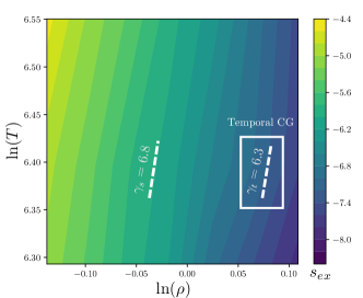
Figure 13: Excess entropy and density scaling exponent estimated from the spatial coarse-graining approach by numerically estimating the $\partial\ln T/\partial\ln\rho$ along curves of constant $S_{\textrm{ex}}$. The single-site CG excess entropy was estimated across various thermodynamic state points using Eq. (V.4.4). Averaging over the illustrated state points gives $\gamma_{s}=6.8$. The value $\gamma_{t}=6.3$ from temporal coarse-graining is shown as a reference (right dashed line).

VI Bottom-Up Density Scaling of OTP and Conclusion

VI.1 Density scaling of dynamics from first principles

In Secs. IV and V, we estimated the density scaling coefficient for molecular OTP using two distinct coarse-graining approaches in time and space. Remarkably, despite originating from different CG descriptions, both approaches yield similar $\gamma$ values. Given its state point dependence, our analysis demonstrates that $\gamma$ varies from 6.3 to 6.8 on average. However, it remains unclear whether this $\gamma$ from our CG description in time and space can correctly capture a one-dimensional phase diagram of OTP from first principles. An indirect yet effective demonstration of density scaling can be realized by estimating the classical Prigogine-Defay ratio, $\Pi$ (Eq. 9). As discussed in the Introduction, strongly correlated systems, i.e., exhibiting an effective single-parameter phase diagram, typically follow $\Pi\approx 1$ Prigogine and R Defay (1954); Gupta and Moynihan (1976); Takahara et al. (1999); Schmelzer and Gutzow (2006); Ellegaard et al. (2007); Pedersen et al. (2008b); Gundermann et al. (2011); Fragiadakis and Roland (2011); Casalini et al. (2011); Tropin et al. (2012); Garden et al. (2012). Therefore, before assessing the density scaling relationship, estimating a $\Pi$ value for OTP from first principles is expected to provide an indirect demonstration of density scaling. Using the computational details outlined in Appendix D, we calculated the $\Pi$ value near the glass transition and found $\Pi=1.02(10)$ (Fig. 14). This value is consistent with the experimental prediction using a similar system as given in Ref. Gundermann et al., 2011 and indirectly supports the existence of the density scaling relationship based on microscopic computer simulations.

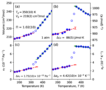
Figure 14: Indirect demonstration of the single-parameter phase diagram of OTP by computing the Prigogine-Defay ratio $\Pi=1.02(10)$ from fully atomistic simulations at the glass transition temperature $T_{g}=350(10)$ K using the jumps of the following response functions between the red and green dashed lines: (a) Average volume in constant $NpT$ simulations, (b) specific isobaric heat capacity, $c_{p}$, (c) isothermal compressibility, $\kappa_{T}$, (d) thermal expansion coefficient, $\alpha_{p}$.

As a final analysis, we now examine whether our approach could provide a correct density scaling using the $\gamma$ determined by the proposed CG approaches. While the experimental success in density scaling of OTP by Tölle motivates this line of investigation Tölle et al. (1998); Tölle (2001), it is unclear if the molecular-level simulation would exhibit this scaling relationship, given that there is no demonstration of density scaling from computer simulations at the fully atomistic level reported in the literature.

In order to perform density scaling from atomistic OTP simulations, we first compute the self-diffusion coefficient from the long-time limit of the atomistic mean square displacement using Einstein’s relation

$$D=\lim_{t\to\infty}\langle(\Delta r(t))^{2}\rangle/6t,$$ (38)

where $\Delta r(t)=|{\bf r}(t)-{\bf r}(0)|$ is the magnitude of the displacement of a given atom within a time-interval $t$, and the average $\langle\ldots\rangle$ is taken over all the atoms and initial times.

The density scaling was then performed by scaling the diffusion coefficients into the inverse reduced diffusion coefficient $1/\tilde{D}=l_{0}^{2}/Dt_{0}$ (where $l_{0}=\rho^{-1/3}$ and $t_{0}=l_{0}\sqrt{m/k_{B}T}$, thus $\tilde{D}$ is dimensionless). Figure 15 illustrates the density scaling relationship of $1/\tilde{D}$ against $1000\rho^{\gamma}/T$, where we used the average density scaling exponent $\gamma=6.5$ from both coarse-graining in space and time. Remarkably, in Fig. 15, we see that the values of the inverse diffusion coefficients collapse onto a master curve, confirming that our CG approach can faithfully capture the density scaling relationship consistent with the experimental findings. We would like to highlight here again that this approach is the first systematic demonstration of density scaling at the molecular level.

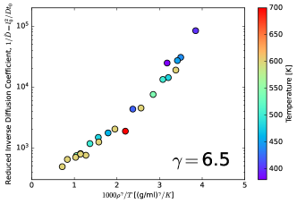
Figure 15: Density scaling of OTP from atomistic simulation, where the dynamical properties from fully atomistic simulations are scaled using the scaling exponent $\gamma=6.5$ determined from both coarse-graining in space and in time over a wide range of temperatures and densities.

VI.2 Summary and Conclusion

In the exploration of soft condensed matter, the thermodynamic scaling relationship emerges as a robust framework capable of predicting the dynamics of a target system across various thermodynamic conditions. While there exist several experimental demonstrations validating this relationship for realistic liquids, a microscopic understanding facilitated by computer simulation currently remains a major challenge. The isomorph theory addresses this gap by tracing out invariant lines (“isomorphs”). However, at a fully atomistic level, the direct application of isomorph theory encounters limitations due to fast intramolecular motions and interactions present in molecules beyond a point particle description. This work aims to bridge the divide between microscopic mechanisms derived from computer simulations and experimental results for the representative glass-forming liquid, OTP.

In order to efficiently explore the free energy landscape of atomistic OTP, we introduced two systematic coarse-graining approaches applied to temporal and spatial domains, each effectively averaging out the fast intramolecular degrees of freedom. In the temporal coarse-graining approach, we time averaged the instantaneous fluctuations of potential energy and virial using a characteristic time scale ranging from 0.1 to 1 ns, enabling the assessment of time-dependent slow fluctuations of OTP molecules. Motivated by experimental successes in measuring frequency-dependent response functions to infer the scaling exponent, we define the frequency-dependent correlation coefficient from correlations between the imaginary parts of signals. Employing the fluctuation-dissipation theorem, we computed the frequency-dependent scaling exponent, resulting in $\gamma=6.3$. For the spatial coarse-graining approach, unimportant intramolecular degrees of freedom are renormalized by reducing the OTP molecule to a single-site center-of-mass representation. The effective interaction at this resolution is purely repulsive, but nevertheless consistent with the ad hoc Lewis-Wahnström model. While the simplified nature of coarse-graining limits our ability to directly evaluate the virial-potential correlations in order to obtain the scaling coefficient, we can circumvent this challenge by tracing out the isomorphs. Leveraging a recent framework to compute the excess entropy of CG molecules, this alternative approach yields a $\gamma$ value of 6.8.

While the two bottom-up coarse-graining approaches stem from different assumptions and underlying microscopic physical principles, a remarkable revelation unfolds: the density scaling coefficients obtained from these two distinct approaches are the same within the numerical uncertainty. Furthermore, utilizing the average $\gamma$ from these coefficients to perform density scaling for the atomistic diffusion coefficients, we confirm that the estimated $\gamma$ imparts the correct scaling relationship across a broad range of temperatures and densities, aligning with experimental observations.

To our knowledge, this work establishes the first bottom-up correspondence to the molecular-level density scaling relationship of realistic materials. Understanding long-time scale dynamical properties on a microscopic level is crucial for advancing predictable multiscale modeling. While this work represents an initial step in this direction, demonstrating the utility and applicability of bottom-up coarse-graining approaches, we expect that our CG framework will apply across various molecular liquids that have been validated experimentally. Moreover, our findings hint at a potential correspondence between the two distinct CG approaches in time and space. The underlying physical principle could be derived from renormalized virials and energetics, and future work will rigorously pursue the first-principles theory to link these distinct CG approaches. Another exciting avenue is to understand excess entropy scaling resulting from these findings. Given that the effective CG description already embodies a reduced interaction nature that is purely repulsive, a systematic approach to deriving the hard sphere-like nature of OTP is expected to extend the density scaling methodology to the excess scaling relationship through a hard sphere mapping. Overall, our framework is poised to facilitate microscopically-informed explorations of the dynamics in complex molecules, ultimately enriching our understanding of the observables from experiments.

Appendices

A. Spatial CG Model of OTP: Single-Site Resolution

1. CG Pair Interactions

To further illustrate the complex nature of bottom-up CG interactions and emphasize the challenges in their inference, Fig. 16 depicts how pair interactions for the spatial CG model of OTP vary with density and temperature. The general trend aligns with our discussion pertinent to Fig. 10, but notably, there is no underlying unified potential in a reduced unit, as is the case with simple analytical interactions. This is because the bottom-up CG interaction includes an entropic contribution, whereas conventional interactions for point particles are purely energetic. For instance, at a fixed volume (constant $NVT$), changes in pair interaction can be understood as the entropic contribution to the CG PMF, as demonstrated by studies of CG liquids. However, the exact forms of entropic and energetic terms for molecular systems involve high-dimensional integrals of FG degrees of freedom, making them challenging to determine.

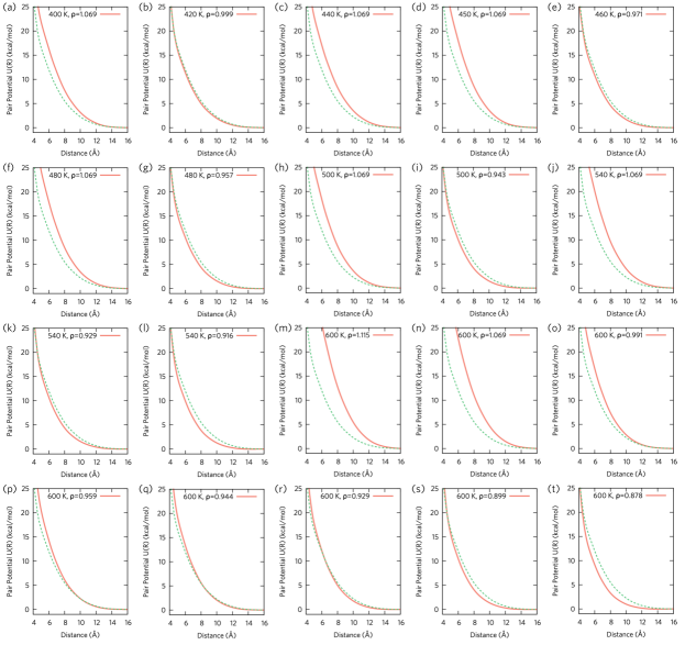
Figure 16: Parametrized pair interactions of the single-site CG OTP at various temperatures and densities using force-matching for the state points except for the one depicted in Fig. 10. Temperature and density conditions are denoted in the title of each panel. For clarity, the CG interaction from Fig. 10(a) is plotted as a reference (green dots) against each CG interaction (red lines).

2. CG Pair Correlations

Similar to Fig. 11, Fig. 17 provides a comprehensive comparison of the pair correlation function between the spatial CG models and the atomistic reference. As discussed in the main text, interestingly, RDFs over different conditions do not seem to differ significantly with drastically different dynamics (as plotted in Fig. 15). This confirms our assertion that higher-order contributions beyond pair excess entropy should be taken into account when computing excess entropy. Our 2PT-based approach was able to distinguish different excess entropy values across these conditions.

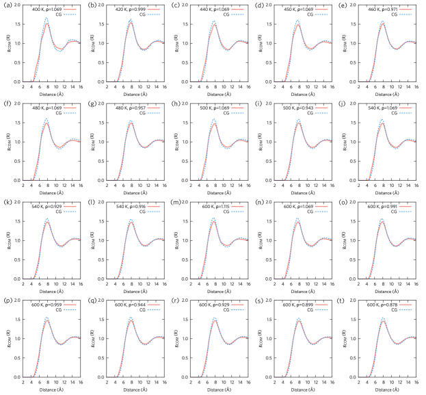
Figure 17: Center-of-mass pair correlation functions $g_{\mathrm{COM}}(R)$ for atomistic (red lines) and the single-site CG (blue dots) simulations of OTP at various temperatures and densities using force-matching for the state points except for the one depicted in Fig. 11. Temperature and density conditions are denoted in the title of each panel.

B. Validation of Spatial Coarse-Graining

We computed the power spectrum $\mathrm{DoS}(\nu)$ from the velocity auto-correlation functions of the atomistic and CG models of OTP to demonstrate that the temporal CG approach can enhance the efficient exploration of the OTP molecules. As expected from the single-site resolution, the CG system only exhibits translational motions, i.e., $v_{\mathrm{CG}}=v_{\mathrm{trans}}$, whereas the atomistic molecules show both translation and vibrational motions: $v_{\mathrm{FG}}=v_{\mathrm{trans}}+v_{\mathrm{rot}}+v_{\mathrm{vib}}$. This difference is shown in Fig. 18, where the CG model only exhibits translational motions at low frequencies below 100 cm^-1. Relatively high-frequency motions, which can be understood as the vibrational motions of OTP molecules, are all removed by coarse-graining. For example, we can identify the non-zero intensities of $\mathrm{DoS}(\nu)$ near 500-1000 cm^-1 as the C-H vibrations of benzene Colthup (2012). A drastic quenching of these vibrational motions, mainly attributed to C-H vibrations, demonstrates the importance of spatial coarse-graining for exploring effective molecular motions in order to identify the virial-potential correlations of OTP.

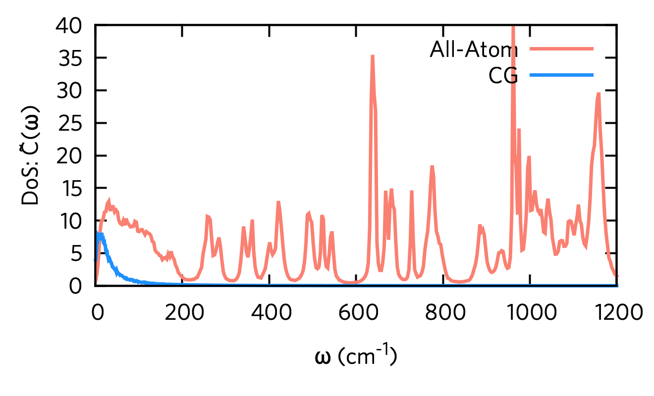
Figure 18: Computed density of states from the velocity auto-correlation functions of atomistic (red) and CG (blue) OTP systems. The obtained DoS$(\omega)=\tilde{C}(\omega)$ is plotted up to 1200 cm${}^{-1},$ corresponding to the fingerprint region of a benzene ring from vibrational spectroscopy Colthup (2012).

C. Assessment of Lewis-Wahnström Model: Thermodynamic Entropy

In order to estimate the overall and intermolecular molar entropy of OTP, we selected the ambient temperature of 360 K under 1 atm conditions, corresponding to a box length of 35.80 Å, as illustrated in Fig. 1(b). Employing the same atomistic simulation protocol as in Section D, 2PT simulations were conducted to calculate the molar entropy.

First, from a fully atomistic simulation, the overall entropy was determined to be 350.54 J/mol/K. Notably, the translational and rotational (intermolecular) contributions at this state point amount to $S_{\textrm{FG}}^{\textrm{trn}}+S_{\textrm{FG}}^{\textrm{rot}}=144.55$ J/K/mol. This indicates that more than half of the entropy arises from the vibrational contribution, underscoring the necessity for careful consideration of the missing entropy when determining the entropy of OTP.

Subsequently, we evaluated the fidelity of the Lewis-Wahnström model by constructing this approximate model under the same system conditions (thermodynamic state point) and conducted MD simulations for 2.5 ns. The 2PT estimation of entropy yielded 149.83 J/K/mol, almost identical to the intermolecular entropy of the atomistic OTP model. This agreement again substantiates our finding that the Lewis-Wahnström model serves as a good approximation for the fully atomistic microscopic model of OTP. Furthermore, our estimated entropy of the Lewis-Wahnström model is in the same order of magnitude as reported earlier in Ref. Mossa et al., 2002 using the inherent structure thermodynamic formalism Stillinger and Weber (1982, 1984) by calculating

$$S(T=360K) =S(T_{0})+3R\log\left(\frac{T=360K}{T_{0}}\right)$$

$$+\int_{T_{0}}^{T=360K}dT^{\prime}\frac{1}{T^{\prime}}\left(\frac{\partial U^{\prime}(T^{\prime})}{\partial T^{\prime}}\right),$$ (39)

where $T_{0}=5000$ K, giving $S(360K)$ approximately 188.75 J/K/mol.

D. Estimation of the Progogine-Defay Ratio

In order to compute the thermodynamic Prigogine-Defay ratio, defined as Prigogine and R Defay (1954); Gupta and Moynihan (1976); Takahara et al. (1999); Schmelzer and Gutzow (2006); Ellegaard et al. (2007); Pedersen et al. (2008b); Gundermann et al. (2011); Fragiadakis and Roland (2011); Casalini et al. (2011); Tropin et al. (2012); Garden et al. (2012)

$$\Pi\equiv\frac{\Delta c_{p}\Delta\kappa_{T}}{V_{g}T_{g}(\Delta\alpha_{p})^{2}},$$ (40)

we conducted the constant $NpT$ simulations at 1 atm for a 200 ns simulation, following 67 ns of equilibration, at different temperatures as illustrated in Fig. 14. The glass transition, identified by changes in slope in Fig. 14(a), was observed on the simulation time scale. Systems near the glass transition that showed partial relaxation (unfilled circles in Fig. 14) were excluded from further analysis. The specific volume at $T_{g}$ was determined as $V_{g}=219(2)$ cm³/mol.

At the glass transition temperature, $\Pi$ was computed from jumps in response functions, utilizing the following equations Allen and Tildesley (1987). The variance of instantaneous enthalpy ($\mathcal{H}+pV$) fluctuations

$$\langle\delta(\mathcal{H}+pV)^{2}\rangle_{NpT}=k_{B}T^{2}c_{p},$$ (41)

was used to estimate the specific isobaric heat capacity $c_{p}$. Then, the variance of volume fluctuations

$$\langle\delta V^{2}\rangle_{NpT}=Vk_{B}T\kappa_{T},$$ (42)

was used to estimate the isothermal compressibility $\kappa_{T}$, and the covariance between volume and enthalpy

$$\langle\delta V\delta(\mathcal{H}+pV)\rangle_{NpT}=k_{B}T^{2}V\alpha_{p},$$ (43)

was used to obtain the thermal expansion coefficient $\alpha_{p}$. From the microscopic OTP simulations, the steps in these response functions at $T_{g}$ were found as $\Delta c_{p}=86(5)$ J/mol$\cdot$K, $\Delta\kappa_{T}=1.75(10)\times 10^{-10}$ Pa^-1, and $\Delta\alpha_{p}=4.42(10)\times 10^{-4}$ K^-1, yielding $\Pi=1.02(10)$ near unity using Eq. 40. Figure 14 further illustrates these jumps in the response functions with the error (i.e., one standard deviation), estimated from Monte Carlo sampling assuming the Gaussian noise.

References

- Chandler (1987) D. Chandler, Introduction to modern statistical mechanics (Oxford University Press, 1987).
- Schroeder (2000) D. V. Schroeder, An introduction to Thermal Physics (Addison Wesley Longman, 2000).
- Roland et al. (2005) C. M. Roland, S. Hensel-Bielowka, M. Paluch, and R. Casalini, Rep. Prog. Phys. 68, 1405 (2005).
- Niss and Hecksher (2018) K. Niss and T. Hecksher, J. Chem. Phys. 149, 230901 (2018).
- Richert (2005) R. Richert, J. Chem. Phys. 123, 154502 (2005).
- Adrjanowicz et al. (2016) K. Adrjanowicz, J. Pionteck, and M. Paluch, RSC Advances 6, 49370 (2016).
- Hansen et al. (2018a) H. W. Hansen, A. Sanz, K. Adrjanowicz, B. Frick, and K. Niss, Nat. Commun. 9, 518 (2018a).
- Tölle et al. (1998) A. Tölle, H. Schober, J. Wuttke, O. G. Randl, and F. Fujara, Phys. Rev. Lett. 80, 2374 (1998).
- Tölle (2001) A. Tölle, Rep. Prog. Phys. 64, 1473 (2001).
- Dreyfus et al. (2003) C. Dreyfus, A. Aouadi, J. Gapinski, M. Matos-Lopes, W. Steffen, A. Patkowski, and R. M. Pick, Phys. Rev. E 68, 011204 (2003).
- Alba-Simionesco et al. (2002) C. Alba-Simionesco, D. Kivelson, and G. Tarjus, J. Chem. Phys. 116, 5033 (2002).
- Fragiadakis and Roland (2011) D. Fragiadakis and C. M. Roland, Phys. Rev. E 83, 031504 (2011).
- Pawlus et al. (2020) S. Pawlus, A. Grzybowski, S. Kołodziej, M. Wikarek, M. Dzida, P. Góralski, S. Bair, and M. Paluch, Sci. Rep. 10, 9316 (2020).
- Hansen et al. (2018b) H. W. Hansen, B. Frick, S. Capaccioli, A. Sanz, and K. Niss, J. Chem. Phys. 149, 214503 (2018b).
- Hansen et al. (2020) H. W. Hansen, F. Lundin, K. Adrjanowicz, B. Frick, A. Matic, and K. Niss, Phys. Chem. Chem. Phys. 22, 14169 (2020).
- Koperwas et al. (2020a) K. Koperwas, A. Grzybowski, and M. Paluch, Phys. Rev. E 101, 012613 (2020a).
- Kauzmann (1948) W. Kauzmann, Chem. Rev. 43, 219 (1948).
- Ediger et al. (1996) M. D. Ediger, C. A. Angell, and S. R. Nagel, J. Phys. Chem. 100, 13200 (1996).
- Angell et al. (2000) C. A. Angell, K. L. Ngai, G. B. McKenna, P. F. McMillan, and S. W. Martin, J. Appl. Phys. 88, 3113 (2000).
- Rosenfeld (1977) Y. Rosenfeld, Phys. Rev. A 15, 2545 (1977).
- Hansen and McDonald (1976) J. P. Hansen and I. McDonald, Theory of Simple Liquids (Academic Press, London, 1976).
- Dyre (2018) J. C. Dyre, J. Chem. Phys. 149, 210901 (2018).
- Lennard-Jones (1924) J. E. Lennard-Jones, Proc. R. Soc. London A 106, 463 (1924).
- Hoover et al. (1971) W. G. Hoover, S. G. Gray, and K. W. Johnson, J. Chem. Phys. 55, 1128 (1971).
- Hoover et al. (1972) W. G. Hoover, D. A. Young, and R. Grover, J. Chem. Phys. 56, 2207 (1972).
- Bernal (1960) J. D. Bernal, Nature 185, 68 (1960).
- Li et al. (2005) G. Li, C. Liu, and Z. Zhu, J. Non-Cryst. Solids 351, 946 (2005).
- Errington et al. (2006) J. R. Errington, T. M. Truskett, and J. Mittal, J. Chem. Phys. 125, 244502 (2006).
- Krekelberg et al. (2007) W. P. Krekelberg, J. Mittal, V. Ganesan, and T. M. Truskett, J. Chem. Phys. 127, 044502 (2007).
- Chakraborty and Chakravarty (2007) S. N. Chakraborty and C. Chakravarty, Phys. Rev. E 76, 011201 (2007).
- Krekelberg et al. (2009) W. P. Krekelberg, M. J. Pond, G. Goel, V. K. Shen, J. R. Errington, and T. M. Truskett, Phys. Rev. E 80, 061205 (2009).
- Chopra et al. (2010) R. Chopra, T. M. Truskett, and J. R. Errington, J. Phys. Chem. B 114, 16487 (2010).
- Mausbach et al. (2018) P. Mausbach, A. Köster, and J. Vrabec, Phys. Rev. E 97, 052149 (2018).
- Hopp et al. (2018) M. Hopp, J. Mele, and J. Gross, Ind. Eng. Chem. Res. 57, 12942 (2018).
- Costigliola et al. (2018) L. Costigliola, U. R. Pedersen, D. M. Heyes, T. B. Schrøder, and J. C. Dyre, J. Chem. Phys. 148, 081101 (2018).
- Costigliola et al. (2019) L. Costigliola, D. M. Heyes, T. B. Schrøder, and J. C. Dyre, J. Chem. Phys. 150, 021101 (2019).
- Bell (2019) I. H. Bell, Proc. Natl. Acad. Sci. U.S.A. 116, 4070 (2019).
- Bell et al. (2020) I. H. Bell, J. C. Dyre, and T. S. Ingebrigtsen, Nat. Commun. 11, 4300 (2020).
- Harris (2020) K. R. Harris, J. Chem. Phys. 153, 104504 (2020).
- Douglas and Xu (2021) J. F. Douglas and W.-S. Xu, Macromolecules 54, 3247 (2021).
- Lötgering-Lin and Gross (2015) O. Lötgering-Lin and J. Gross, Ind. Eng. Chem. Res. 54, 7942 (2015).
- Lötgering-Lin et al. (2018) O. Lötgering-Lin, M. Fischer, M. Hopp, and J. Gross, Ind. Eng. Chem. Res. 57, 4095 (2018).
- Baled et al. (2018) H. O. Baled, I. K. Gamwo, R. M. Enick, and M. A. McHugh, Fuel 218, 89 (2018).
- Rokni et al. (2019) H. B. Rokni, J. D. Moore, A. Gupta, M. A. McHugh, and M. Gavaises, Fuel 241, 1203 (2019).
- Taib and Trusler (2020) M. B. M. Taib and J. P. M. Trusler, J. Chem. Phys. 152, 164104 (2020).
- Liu et al. (2020) H. Liu, F. Yang, Z. Yang, and Y. Duan, Journal of Molecular Liquids 308, 113027 (2020).
- Bell (2020a) I. H. Bell, J. Chem. Eng. Data 65, 3203 (2020a).
- Bell (2020b) I. H. Bell, J. Chem. Eng. Data 65, 5606 (2020b).
- Yang et al. (2021) X. Yang, X. Xiao, E. F. May, and I. H. Bell, J. Chem. Eng. Data 66, 1385 (2021).
- Bell et al. (2022) I. H. Bell, R. Fingerhut, J. Vrabec, and L. Costigliola, J. Chem. Phys. 157, 074501 (2022).
- Jin et al. (2023a) J. Jin, K. S. Schweizer, and G. A. Voth, J. Chem. Phys. 158, 034103 (2023a).
- Jin et al. (2023b) J. Jin, K. S. Schweizer, and G. A. Voth, J. Chem. Phys. 158, 034104 (2023b).
- Jin et al. (2023c) J. Jin, E. K. Lee, and G. A. Voth, J. Chem. Phys. 159, 164102 (2023c).
- Ghaffarizadeh and Wang (2022) S. A. Ghaffarizadeh and G. J. Wang, J. Phys. Chem. Lett. 13, 4949 (2022).
- Saw et al. (2023) S. Saw, L. Costigliola, and J. C. Dyre, Phys. Rev. E 107, 024609 (2023).
- Widom (1967a) B. Widom, Science 157, 375 (1967a).
- Weeks et al. (1971) J. D. Weeks, D. Chandler, and H. C. Andersen, J. Chem. Phys. 54, 5237 (1971).
- Widom (1967b) B. Widom, Science 157, 375 (1967b).
- Greet and Turnbull (1967) R. J. Greet and D. Turnbull, J. Chem. Phys. 46, 1243 (1967).
- Takahara et al. (1999) S. Takahara, M. Ishikawa, O. Yamamuro, and T. Matsuo, J. Phys. Chem. B 103, 792 (1999).
- Casalini et al. (2016) R. Casalini, S. S. Bair, and C. M. Roland, J. Chem. Phys. 145, 064502 (2016).
- Mapes et al. (2006) M. K. Mapes, S. F. Swallen, and M. D. Ediger, J. Phys. Chem. B 110, 507 (2006).
- Gnan et al. (2009) N. Gnan, T. B. Schrøder, U. R. Pedersen, N. P. Bailey, and J. C. Dyre, J. Chem. Phys. 131, 234504 (2009).
- Schrøder et al. (2011) T. B. Schrøder, N. Gnan, U. R. Pedersen, N. P. Bailey, and J. C. Dyre, J. Chem. Phys. 134, 164505 (2011).
- Mandelbrot and Ness (1968) B. B. Mandelbrot and J. W. V. Ness, SIAM Review 10, 422 (1968).
- Guth and Pi (1982) A. H. Guth and S.-Y. Pi, Phys. Rev. Lett. 49, 1110 (1982).
- Hawking (1982) S. Hawking, Phys. Lett. B 115, 295 (1982).
- (68) B. B. Mandelbrot, The Fractal Geometry of Nature (Freeman).
- Pelissetto and Vicari (2002) A. Pelissetto and E. Vicari, Phys. Rep. 368, 549 (2002).
- Bak et al. (2002) P. Bak, K. Christensen, L. Danon, and T. Scanlon, Phys. Rev. Lett. 88, 178501 (2002).
- Schrøder and Dyre (2014) T. B. Schrøder and J. C. Dyre, J. Chem. Phys. 141, 204502 (2014).
- Dyre (2014) J. C. Dyre, J. Phys. Chem. B. 118, 10007 (2014), pMID: 25011702.
- Alba-Simionesco et al. (2004) C. Alba-Simionesco, A. Cailliaux, A. Alegria, and G. Tarjus, EPL 68, 58 (2004).
- Casalini and Roland (2004) R. Casalini and C. M. Roland, Phys. Rev. E 69 (2004), 10.1103/physreve.69.062501.
- Pedersen et al. (2008a) U. R. Pedersen, N. P. Bailey, T. B. Schrøder, and J. C. Dyre, Phys. Rev. Lett. 100, 015701 (2008a).
- Pedersen et al. (2010a) U. R. Pedersen, T. B. Schrøder, and J. C. Dyre, Phys. Rev. Lett. 105, 157801 (2010a).
- Hummel et al. (2015) F. Hummel, G. Kresse, J. C. Dyre, and U. R. Pedersen, Phys. Rev. B 92, 174116 (2015).
- Heyes (1998) D. M. Heyes, The Liquid State. Applications of Molecular Simulations (Wiley Series in Theoretical Chemistry, 1998).
- Frenkel and Smit (2002) D. Frenkel and B. Smit, Understanding molecular simulation: from algorithms to applications, 2nd ed. (Academic Press, 2002).
- Bailey et al. (2008a) N. P. Bailey, U. R. Pedersen, N. Gnan, T. B. Schrøder, and J. C. Dyre, J. Chem. Phys. 129, 184507 (2008a).
- Bailey et al. (2008b) N. P. Bailey, U. R. Pedersen, N. Gnan, T. B. Schrøder, and J. C. Dyre, J. Chem. Phys. 129, 184508 (2008b).
- Gundermann et al. (2011) D. Gundermann, U. R. Pedersen, T. Hecksher, N. P. Bailey, B. Jakobsen, T. Christensen, N. B. Olsen, T. B. Schrøder, D. Fragiadakis, R. Casalini, C. M. Roland, J. C. Dyre, and K. Niss, Nature Phys. 7, 816 (2011).
- Bacher et al. (2018) A. K. Bacher, T. B. Schrøder, and J. C. Dyre, J. Chem. Phys. 149, 114502 (2018).
- Bacher et al. (2020) A. K. Bacher, U. R. Pedersen, T. B. Schrøder, and J. C. Dyre, J. Chem. Phys. 152, 094505 (2020).
- Schrøder et al. (2009) T. B. Schrøder, U. R. Pedersen, N. P. Bailey, S. Toxvaerd, and J. C. Dyre, Phys. Rev. E 80, 041502 (2009).
- Hu et al. (2016) Y.-C. Hu, B.-S. Shang, P.-F. Guan, Y. Yang, H.-Y. Bai, and W.-H. Wang, J. Chem. Phys. 145, 104503 (2016).
- Friedeheim et al. (2019) L. Friedeheim, J. C. Dyre, and N. P. Bailey, Phys. Rev. E 99, 022142 (2019).
- Singh et al. (2021) A. Singh, J. Dyre, and U. R. Pedersen, J. Chem. Phys. 154, 134501 (2021).
- Pedersen et al. (2010b) U. R. Pedersen, G. H. Peters, T. B. Schrøder, and J. C. Dyre, J. Phys. Chem. B 114, 2124 (2010b).
- Ingebrigtsen et al. (2012) T. S. Ingebrigtsen, T. B. Schrøder, and J. C. Dyre, J. Phys. Chem. B 116, 1018 (2012).
- Veldhorst et al. (2015) A. A. Veldhorst, J. C. Dyre, and T. B. Schrøder, J. Chem. Phys. 143, 194503 (2015).
- Koperwas et al. (2020b) K. Koperwas, A. Grzybowski, and M. Paluch, Phys. Rev. E 102, 062140 (2020b).
- Veldhorst et al. (2014) A. A. Veldhorst, J. C. Dyre, and T. B. Schrøder, J. Chem. Phys. 141, 054904 (2014).
- Goldstein (1969) M. Goldstein, J. Chem. Phys. 51, 3728 (1969).
- Ediger and Harrowell (2012) M. D. Ediger and P. Harrowell, J. Chem. Phys. 137, 080901 (2012).
- Biroli and Garrahan (2013) G. Biroli and J. P. Garrahan, J. Chem. Phys. 138, 12A301 (2013).
- Prigogine and R Defay (1954) I. Prigogine and R. R Defay, Chemical Thermodynamics (Longman, 1954).
- Gupta and Moynihan (1976) P. K. Gupta and C. T. Moynihan, J. Chem. Phys. 65, 4136 (1976).
- Schmelzer and Gutzow (2006) J. W. P. Schmelzer and I. Gutzow, J. Chem. Phys. 125, 184511 (2006).
- Ellegaard et al. (2007) N. L. Ellegaard, T. Christensen, P. V. Christiansen, N. B. Olsen, U. R. Pedersen, T. B. Schrøder, and J. C. Dyre, J. Chem. Phys. 126, 074502 (2007).
- Pedersen et al. (2008b) U. R. Pedersen, T. Christensen, T. B. Schrøder, and J. C. Dyre, Phys. Rev. E 77, 011201 (2008b).
- Casalini et al. (2011) R. Casalini, R. F. Gamache, and C. M. Roland, J. Chem. Phys. 135, 224501 (2011).
- Tropin et al. (2012) T. V. Tropin, J. W. P. Schmelzer, I. Gutzow, and C. Schick, J. Chem. Phys. 136, 124502 (2012).
- Garden et al. (2012) J.-L. Garden, H. Guillou, J. Richard, and L. Wondraczek, J. Non-Equilib. Thermodyn. 37, 143 (2012).
- Wahnström and Lewis (1993) G. Wahnström and L. J. Lewis, Physica A 201, 150 (1993).
- Lewis and Wahnström (1993) L. J. Lewis and G. Wahnström, Solid State Commun. 86, 295 (1993).
- Lewis and Wahnström (1994) L. J. Lewis and G. Wahnström, J. Non-Cryst. Solids 172, 69 (1994).
- Lewis and Wahnström (1994) L. J. Lewis and G. Wahnström, Phys. Rev. E 50, 3865 (1994).
- Wahnström and Lewis (1997) G. Wahnström and L. J. Lewis, Suppl. Prog. Theor. Phys. 126, 261 (1997).
- Rinaldi et al. (2001) A. Rinaldi, F. Sciortino, and P. Tartaglia, Phys. Rev. E 63, 061210 (2001).
- Lombardo et al. (2006) T. G. Lombardo, P. G. Debenedetti, and F. H. Stillinger, J. Chem. Phys. 125, 174507 (2006).
- Pedersen et al. (2011) U. R. Pedersen, T. S. Hudson, and P. Harrowell, J. Chem. Phys. 134, 114501 (2011).
- Müller-Plathe (2002) F. Müller-Plathe, ChemPhysChem 3, 754 (2002).
- Voth (2008) G. A. Voth, Coarse-graining of condensed phase and biomolecular systems (CRC press, 2008).
- Peter and Kremer (2009) C. Peter and K. Kremer, Soft Matter 5, 4357 (2009).
- Noid (2013) W. G. Noid, J. Chem. Phys. 139, 090901 (2013).
- Brini et al. (2013) E. Brini, E. A. Algaer, P. Ganguly, C. Li, F. Rodríguez-Ropero, and N. F. van der Vegt, Soft Matter 9, 2108 (2013).
- Jin et al. (2022) J. Jin, A. J. Pak, A. E. Durumeric, T. D. Loose, and G. A. Voth, J. Chem. Theory Comput. 18, 5759 (2022).
- Dodda et al. (2017) L. S. Dodda, J. Z. Vilseck, J. Tirado-Rives, and W. L. Jorgensen, J. Phys. Chem. B 121, 3864 (2017).
- Grønbech-Jensen and Farago (2014) N. Grønbech-Jensen and O. Farago, J. Chem. Phys. 141, 194108 (2014).
- Grønbech-Jensen et al. (2014) N. Grønbech-Jensen, N. R. Hayre, and O. Farago, Comput. Phys. Commun. 185, 524 (2014).
- Thompson et al. (2022) A. P. Thompson, H. M. Aktulga, R. Berger, D. S. Bolintineanu, W. M. Brown, P. S. Crozier, P. J. in ’t Veld, A. Kohlmeyer, S. G. Moore, T. D. Nguyen, R. Shan, M. J. Stevens, J. Tranchida, C. Trott, and S. J. Plimpton, Comp. Phys. Comm. 271, 108171 (2022).
- Virtanen et al. (2020) P. Virtanen, R. Gommers, T. E. Oliphant, M. Haberland, T. Reddy, D. Cournapeau, E. Burovski, P. Peterson, W. Weckesser, J. Bright, S. J. van der Walt, M. Brett, J. Wilson, K. J. Millman, N. Mayorov, A. R. J. Nelson, E. Jones, R. Kern, E. Larson, C. J. Carey, İ. Polat, Y. Feng, E. W. Moore, J. VanderPlas, D. Laxalde, J. Perktold, R. Cimrman, I. Henriksen, E. A. Quintero, C. R. Harris, A. M. Archibald, A. H. Ribeiro, F. Pedregosa, P. van Mulbregt, and SciPy 1.0 Contributors, Nature Methods 17, 261 (2020).
- Press et al. (2007) W. H. Press, S. A. Teukolsky, W. T. Vetterling, and B. P. Flannery, Numerical Recipes 3rd Edition: The Art of Scientific Computing, 3rd ed. (Cambridge University Press, USA, 2007).
- Pedersen (2009) U. R. Pedersen, “Ph.d. thesis: Long-time simulations of viscous liquids,” (2009).
- Nielsen and Dyre (1996) J. K. Nielsen and J. C. Dyre, Phys. Rev. B 54, 15754 (1996).
- Noid et al. (2008a) W. G. Noid, J.-W. Chu, G. S. Ayton, V. Krishna, S. Izvekov, G. A. Voth, A. Das, and H. C. Andersen, J. Chem. Phys. 128, 244114 (2008a).
- Noid et al. (2008b) W. Noid, P. Liu, Y. Wang, J.-W. Chu, G. S. Ayton, S. Izvekov, H. C. Andersen, and G. A. Voth, J. Chem. Phys. 128, 244115 (2008b).
- Dunn et al. (2016) N. J. Dunn, T. T. Foley, and W. G. Noid, Acc. Chem. Res. 49, 2832 (2016).
- Jin et al. (2019) J. Jin, A. J. Pak, and G. A. Voth, J. Phys. Chem. Lett. 10, 4549 (2019).
- Jin et al. (2020) J. Jin, A. Yu, and G. A. Voth, J. Chem. Theory Comput. 16, 6823 (2020).
- Lu et al. (2010) L. Lu, S. Izvekov, A. Das, H. C. Andersen, and G. A. Voth, J. Chem. Theory Comput. 6, 954 (2010).
- Noid et al. (2007) W. Noid, J.-W. Chu, G. S. Ayton, and G. A. Voth, J. Phys. Chem. B 111, 4116 (2007).
- Peng et al. (2023) Y. Peng, A. J. Pak, A. E. P. Durumeric, P. G. Sahrmann, S. Mani, J. Jin, T. D. Loose, J. Beiter, and G. A. Voth, J. Phys. Chem. B 127, 8537 (2023).
- Press (2007) W. H. Press, Numerical recipes 3rd edition: The art of scientific computing (Cambridge University Press, 2007).
- Allen and Rutledge (2009) E. C. Allen and G. C. Rutledge, J. Chem. Phys. 130, 034904 (2009).
- Lu and Voth (2011) L. Lu and G. A. Voth, J. Chem. Phys. 134, 224107 (2011).
- Hsu et al. (2015) D. D. Hsu, W. Xia, S. G. Arturo, and S. Keten, Macromolecules 48, 3057 (2015).
- Johnson et al. (2007) M. E. Johnson, T. Head-Gordon, and A. A. Louis, J. Chem. Phys. 126, 144509 (2007).
- Wagner et al. (2016) J. W. Wagner, J. F. Dama, A. E. Durumeric, and G. A. Voth, J. Chem. Phys. 145, 044108 (2016).
- Dannenhoffer-Lafage et al. (2019) T. Dannenhoffer-Lafage, J. W. Wagner, A. E. Durumeric, and G. A. Voth, J. Chem. Phys. 151, 134115 (2019).
- Wallace (1987) D. C. Wallace, Phys. Lett. A 122, 418 (1987).
- Baranyai and Evans (1989) A. Baranyai and D. J. Evans, Phys. Rev. A 40, 3817 (1989).
- Green (1952) H. S. Green, Molecular theory of fluids (North-Holland, Amsterdam, 1952).
- Kumar et al. (2009) P. Kumar, S. V. Buldyrev, and H. E. Stanley, Proc. Natl. Acad. Sci. U.S.A. 106, 22130 (2009).
- Cisneros et al. (2016) G. A. Cisneros, K. T. Wikfeldt, L. Ojamaäe, J. Lu, Y. Xu, H. Torabifard, A. P. Bartók, G. Csányi, V. Molinero, and F. Paesani, Chem. Rev. 116, 7501 (2016).
- Lazaridis and Karplus (1996) T. Lazaridis and M. Karplus, J. Chem. Phys. 105, 4294 (1996).
- Lazaridis (2000) T. Lazaridis, J. Phys. Chem. B 104, 4964 (2000).
- Zielkiewicz (2008) J. Zielkiewicz, J. Phys. Chem. B 112, 7810 (2008).
- Vera and Prausnitz (1972) J. Vera and J. Prausnitz, Chem. Eng. J. 3, 1 (1972).
- Sandler (1985) S. I. Sandler, Fluid Phase Equilib. 19, 238 (1985).
- Abbott and Prausnitz (1987) M. M. Abbott and J. M. Prausnitz, Fluid Phase Equilib. 37, 29 (1987).
- Jin and Reichman (2023) J. Jin and D. R. Reichman, “Hierarchical framework for predicting entropies in bottom-up coarse-grained models,” (2023), arXiv:2311.12353 [physics.chem-ph] .
- Lin et al. (2003) S.-T. Lin, M. Blanco, and W. A. Goddard III, J. Chem. Phys. 119, 11792 (2003).
- Lin et al. (2010) S.-T. Lin, P. K. Maiti, and W. A. Goddard III, J. Phys. Chem. B 114, 8191 (2010).
- Pascal et al. (2011) T. A. Pascal, S.-T. Lin, and W. A. Goddard III, Phys. Chem. Chem. Phys. 13, 169 (2011).
- Jin and Goddard III (2015) J. Jin and W. A. Goddard III, J. Phys. Chem. C 119, 2622 (2015).
- Karplus and Kushick (1981) M. Karplus and J. N. Kushick, Macromolecules 14, 325 (1981).
- Carnahan and Starling (1970) N. F. Carnahan and K. E. Starling, J. Chem. Phys. 53, 600 (1970).
- Chapman and Cowling (1990) S. Chapman and T. G. Cowling, The mathematical theory of non-uniform gases: an account of the kinetic theory of viscosity, thermal conduction and diffusion in gases (Cambridge University Press, 1990).
- Chang and Bestul (1972) S. Chang and A. Bestul, J. Chem. Phys. 56, 503 (1972).
- McQuarrie and Simon (1997) D. A. McQuarrie and J. D. Simon, Physical chemistry: a molecular approach, Vol. 1 (University science books Sausalito, CA, 1997).
- Colthup (2012) N. Colthup, Introduction to infrared and Raman spectroscopy (Elsevier, 2012).
- Mossa et al. (2002) S. Mossa, E. La Nave, H. Stanley, C. Donati, F. Sciortino, and P. Tartaglia, Phys. Rev. E 65, 041205 (2002).
- Stillinger and Weber (1982) F. H. Stillinger and T. A. Weber, Phys. Rev. A 25, 978 (1982).
- Stillinger and Weber (1984) F. H. Stillinger and T. A. Weber, Science 225, 983 (1984).
- Allen and Tildesley (1987) M. Allen and D. Tildesley, Computer Simulation of Liquids (Oxford University Press, 1987).