Tunable shape oscillations of adaptive droplets

Abstract

Living materials adapt their shape to signals from the environment, yet the impact of shape changes on signal processing and the associated feedback dynamics remain unclear. We derive coarse-grained equations for droplets that adjust their interfacial tension in response to signals exchanged at contact surfaces, from the microscopic biophysics of adhesion and signaling. We find that droplet pairs exhibit symmetry-breaking, excitability, and oscillations. The underlying critical points reveal novel mechanisms for physical signal processing through shape adaptation in soft active materials.

Dynamic and non-trivial geometries are hallmarks of soft active matter, because intrinsic stress fields drive autonomous shape changes in deformable materials [1, 2, 3, 4, 5]. In turn, boundary geometry can influence stresses and material properties, or determine how macroscopic work is extracted from microscopic sources of activity [6, 7]. Some complex materials process signals and adaptively respond to their environment [8, 9, 10]. Geometry-dependent feedback arises when signal processing depends on the system’s shape.

In particular living materials possess internal degrees of freedom that adjust their mechanical properties in response to peripheral signals. In cells, signals trigger biochemical processes including the regulation of gene expression that control the molecular composition in the bulk and at the surface [11]. Inhibitory signaling interactions between neighboring cells for example lead to the spontaneous symmetry-breaking of such internal states, giving rise to distinctly shaped cell types [12, 13]. The resulting mechanochemical feedback dynamics govern the spatial organisation of diverse multicellular systems [14, 15, 16].

We propose that geometry-dependent feedback effects generically underlie the capacity of soft active systems to autonomously solve tasks including locomotion [17, 18, 19, 20], self-healing [21, 22], and the self-organisation of complex structures [23, 24, 25]. Yet, how internal cellular states interact with shape dynamics is an open question [26, 27, 25], and more generally, how the phase space of adaptive shape-changing materials depends on geometry is unclear.

Uncovering the theoretical principles governing the rich physics of adaptive active matter systems requires minimal, tractable paradigms. Here, we consider adaptive droplets that change their surface tension in response to signals received at contact surfaces with other droplets or substrates. Particularly interesting dynamics appear for mutually inhibitory interactions, i.e. when signals received by a droplet reduce its own capacity to send signals. To analyse how nonlinear signal processing interplays with fundamental nonlinearities in geometrical relations, we derive a minimal set of equations governing the macroscopic droplet states, controlled by two dimensionless feedback parameters. These equations are consistent with microscopic reaction-diffusion dynamics of signaling and adhesion molecules (SM [28], Sec. .1). We show that coupling between active mechanics and signaling creates a variety of nonlinear phenomena, including bistability, excitability, and diverse oscillations of droplet shapes and internal states, which arise from a saddle-node pitchfork codimension-2 bifurcation point.

Adaptive Young-Laplace droplets.—

We consider a pair of Young-Laplace droplets with interfacial areas governed by the conjugate uniform surface tensions at fixed volumes [Fig. 1(a)]. The total surface energy for a pair of identical droplets is

$$E=\gamma_{\rm{c}}A_{\rm{c}}+2\gamma_{\rm{f}}A_{\rm{f}},$$ (1)

in which $\gamma_{\rm{c}}$ and $\gamma_{\rm{f}}$ are the surface tensions of the contact interface $A_{\rm{c}}$ and the outer surface area $A_{\rm{f}}$, respectively. For positive interfacial tensions, the surface energy is minimal when both droplets acquire a spherical-cap shape with contact area

$$\dfrac{A_{\rm{c}}}{A_{0}}=\left[1-\left(\frac{\gamma_{\rm{c}}}{2\gamma_{\rm{f}}}\right)^{2}\right]\left[\dfrac{2}{\left(2-\dfrac{\gamma_{\rm{c}}}{2\gamma_{\rm{f}}}\right)\left(1+\dfrac{\gamma_{\rm{c}}}{2\gamma_{\rm{f}}}\right)^{2}}\right]^{\frac{2}{3}}$$ (2)

relative to the reference area $A_{0}=(3V/2)^{2/3}\pi^{1/3}$ determined by the conserved volumes $V_{1}=V_{2}=V$ [Fig. 1(c)].

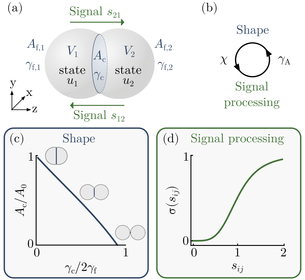
Figure 1: (a) We consider equilibrium shapes of Young-Laplace droplet pairs, which adapt the tension $\gamma_{\rm{c}}$ at their contact surface $A_{\rm{c}}$ to their internal states $u_{1},u_{2}$. The droplets have conserved volumes $V_{1},V_{2}$ and uniform outer surface tensions $\gamma_{\rm{f},1},\gamma_{\textrm{f},2}$ at the outer surfaces $A_{\textrm{f},1},A_{\textrm{f},2}$. (b) The signal susceptibility $\chi$ and the adaptive adhesion coefficient $\gamma_{\rm{A}}$ govern the feedback between shape and signal processing (c) The equilibrium contact area depends on tension ratio $\gamma_{\rm{c}}/2\gamma_{\rm{f}}$—shown here for equal volumes and outer surface tensions [Eq. (2)]—and sets the magnitude of the exchanged signals [Eq. (5)]. (d) The internal states evolve according to mutually inhibitory interactions [Eq. (4)-(5)], with a sigmoidal response function $\sigma(s_{ij})=s_{ij}^{4}/(s_{ij}^{4}+1)$.

We take the adhesion between the droplets to depend on the signals exchanged at their shared surface. Therefore, to each droplet $i\in\{1,2\}$ we assign a dimensionless internal state $u_{i}\in[0,1]$, a variable that increases in response to received signals in a saturating manner [Fig. 1(d),[29, 16, 30]]. When the internal state drives active processes that increase the adhesion between the droplets, a first-order relation linking the tension at the droplet-droplet interface and the internal states can be written as

$$\gamma_{\rm{c}}=\gamma_{0}-\gamma_{\rm{A}}u_{1}u_{2},$$ (3)

in which the second term contains the active contributions in response to signaling, while $\gamma_{0}$ contains all other components of the interfacial tension. A variety of active microscopic processes can modulate the effective tension at the surface of cells, including the generation of stresses by molecular motors within polymerizing cytoskeletal networks [31, 32, 33] and biochemical regulation of adhesion [34, 35, 36]. We derive Eq. (3) considering a signal-driven production of adhesive molecules within the droplets’ bulk and the steady-state reaction kinetics of adhesion complexes forming at the contact interface ([28], Sec. .2). The product of internal states in the adaptive tension arises for mass-action reaction kinetics, and a linear dependence of adhesion molecule production in the bulk on the internal states. The adaptive adhesion coefficient $\gamma_{\rm{A}}$ captures the strength of the coupling between the internal states and the interfacial tension. Because adhesion reduces the tension, the adaptive term is always negative. It can be expressed as $\gamma_{\rm{A}}=\epsilon/\lambda^{2}$ in terms of an energy per adhesion complex $\epsilon$ and a length scale $\lambda$ dependent on the rate of turnover at the bulk-surface interface (Eq. (76) in [28]). Similar relationships between the molecular composition—for instance the concentration of molecular motors—and stresses at the cell surface have been used successfully to describe tension fields and predict associated flows and shape changes in living systems [37, 38, 39]. The adaptive tension vanishes in the absence of signaling interactions and it always acts to increase the interfacial area $A_{\rm{c}}(\gamma_{0})\leq A_{\rm{c}}(\gamma_{\rm{c}})$ [Eq. (2)] up to the limit set by the saturation of the internal states. A very large adaptive adhesion coefficient leads to a buckling instability of the interface when $\gamma_{\rm{c}}<0$ – an increase in the interface area then decreases the surface energy [40, 5]. Our analysis focuses on the regime $\gamma_{\rm{A}}<\gamma_{0}$ in which Eq. (2) is valid.

The states of the droplets $u_{i}$ are taken to evolve according to a generic mutually inhibitory signaling interaction [16, 30]

$$\tau_{\rm{u}}\frac{du_{i}}{dt}=\sigma(s_{ij})-u_{i},$$ (4)

in which $\sigma(s_{ij})$ is an increasing sigmoidal response function to a signal $s_{ij}$ received by droplet $i$ from droplet $j$ [Fig. 1(d)]. We use a Hill function $\sigma(s_{ij})=s_{ij}^{h}/(s_{ij}^{h}+1)$ with Hill coefficient $h=4$ [41, 42]. The magnitude of $s_{ij}$ depends on the internal state of the sending droplet $u_{j}$ and—for mutually inhibitory coupling—must decrease with $u_{j}$. We use in the following a first-order relation taking into account a linear dependence of the exchanged signals on the contact area [43, 44]

$$s_{ij}=\chi\frac{A_{\rm{c}}}{A_{0}}(1-u_{j})$$ (5)

with a dimensionless signal susceptibility parameter $\chi$. Equations (4)–(5) can be derived from reaction-diffusion dynamics of biochemical signaling molecules ([28], Sec. .3.2) in which $u_{i}$ is defined as a rescaled and normalized concentration of a regulator molecule, such as a transcription factor. These microscopic equations relate $\chi$ to the kinetic rates associated with the turnover, binding, and processing of signaling molecules. [Eq. (43),(74) in [28]]. The linear dependence of transmitted molecular signals on the contact area is valid when diffusion across the contact line and the number of molecules lost through biochemical processes at the surface are negligible.

Provided that the adaptive droplet pairs relax to their equilibrium configuration fast compared to the signaling time scale $\tau_{\rm{u}}$ and the corresponding change in the interfacial tension, the coupled dynamics of the doublet are governed by Eqs. (2)–(5). Two coupling coefficients characterize the feedback between the system’s geometry and the internal states: the adaptive adhesion coefficient $\gamma_{\rm{A}}$ controls the effect of signaling on the surface mechanics and thereby shape, and the signal susceptibility $\chi$ captures how transmitted signals depend on the contact area [Fig. 1(b)].

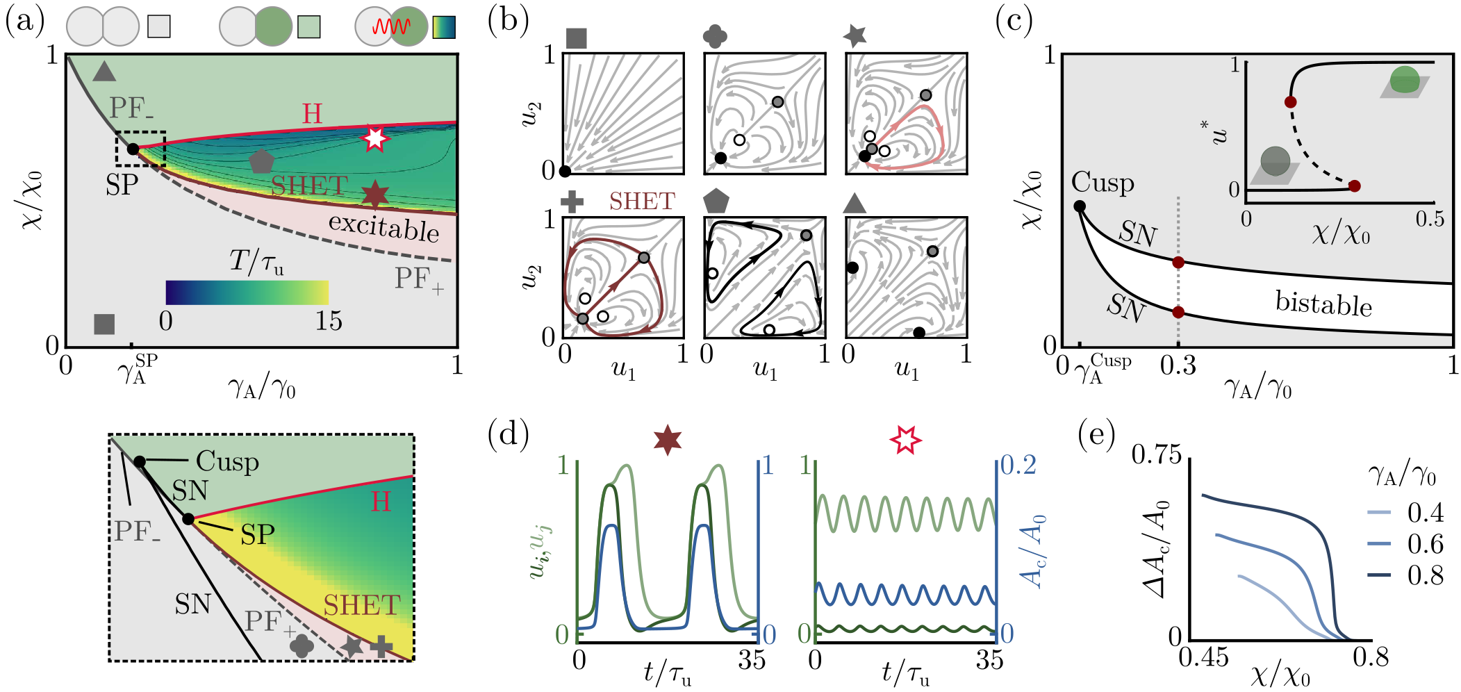
Figure 2: Nonlinear dynamics of adaptive Young-Laplace droplet pairs. (a) The droplet pair state diagram shows that tension adaptation increases the parameter regime (green) associated with spontaneous symmetry-breaking due to mutual inhibition (PF_-: supercritical pitchfork PF₊: subcritical pitchfork), and leads to self-sustained oscillations of signals and droplet shapes (color gradient and contour lines denote the oscillation period $T$). The oscillatory regime is surrounded by saddle-heteroclinic (SHET) and Hopf (H) bifurcation lines that originate from a saddle-node pitchfork codimension-2 point (SP). Bottom panel: Enlarged view of the SP point environment shows saddle-node (SN) and cusp bifurcations that preserve stable attractor structures. The reference susceptibility is the critical value in the absence of adaptive tension ($\chi_{0}=\left.\chi_{\rm{PF}}\right|_{\gamma_{\rm{A}}=0}$). (b) The state diagram of a single adherent droplet on a signal-transmitting substrate contains a bistable regime bounded by two SN lines that originate from a codimension-2 cusp point. Inset: steady-state internal state as a function of the signal susceptibility (along gray dashed line) (c) Phase portraits for parameter values marked with gray symbols (filled black circle: stable steady state, filled gray circle: saddle, open circle: unstable steady state, rose line: trajectory in the excitable regime, red line: heteroclinic, black line: limit cycle). (d-e) Oscillation amplitudes decrease with waveforms changing from relaxation-like (near the SHET line) to sinusoidal (near the Hopf line) for increasing $\chi$. Parameter values given in [28], Tab. 2.

Adaptive tension promotes symmetry-breaking.—

Strong mutually inhibitory interactions generically lead to spontaneous symmetry-breaking, whereby initially small differences between interacting units diverge to high- and low-value steady states [12]. Linear stability analysis, numerical continuation, and simulations of Eqs. (2)–(5) reveal that pairs of adaptive droplets undergo symmetry-breaking of internal states via a line of supercritical pitchfork bifurcations (PF) in the state diagram spanned by the signal susceptibility $\chi$ and the adaptive adhesion coefficient $\gamma_{\rm{A}}$ [Fig. 2(a-b)]. Below the critical value $\chi_{\rm{PF}}$, inhibition is not sufficient to produce symmetry-breaking, and the two droplets converge to identical internal states near zero in a configuration with a small contact. The critical susceptibility scales approximately inversely with the interfacial area $\chi_{\rm{PF}}\sim A_{0}/A_{c}$ ([28], Sec. .3.2). Thus, adhesive tension adaptation promotes symmetry-breaking: the active term in Eq. (3) transiently expands the contact area, thereby lowering the threshold susceptibility. This shows that adaptive shape changes enable state transitions beyond the parameter regime attainable in static configurations.

Tunable self-sustained oscillations.—

At large adaptive tension, the coupling between signaling and interface geometry leads to diverse self-sustained oscillations in the shape of the droplet pair and the internal states. Specifically, stable symmetric and symmetry-broken states are separated by an oscillatory regime, bounded by Hopf (H) and saddle heteroclinic (SHET) bifurcation lines [Fig. 2(a-b)]. These lines originate from a saddle-node pitchfork bifurcation point (SP)—a codimension-2 bifurcation at which the PF line tangentially intersects with a saddle-node (SN) bifurcation line [[28], Fig. 13] [45]. In this region, the coupling between interface area and transmitted signals [Eqs. (3)–(5)] gives rise to a bistability between small and large contact area configurations, which competes with the tendency of the droplet pair to undergo symmetry-breaking of internal states. A negative feedback arises between the product of states $u_{1}u_{2}$—which increases the contact area via Eq. 3—and the contact area across which inhibition occurs.

This area bistability is exhibited also by single adherent droplets on signal-transmitting substrates [[28], Sec. .3.1], where the state diagram contains two SN lines that originate from a codimension-2 cusp point [Fig. 2(c) and [28], Sec. .3.1]. Above a critical susceptibility, the positive feedback between signaling and adhesion enables two stable configurations: since the contact area limits the amplitude of adhesion-inducing signals from the substrate, a droplet with a small contact area remains weakly adhesive, whereas a large contact area permits the transmission of strong signals, promoting substrate wetting. At large susceptibilities, the bistability is lost, and the configuration with large contact area remains the only steady state.

In the two-dimensional phase space of the droplet pair, the SN bifurcation associated with the area bistability produces a saddle point and an unstable fixed point instead of the pair of stable and unstable fixed points observed in the single-droplet system [Fig. 2(b) quatrefoil]. When $\gamma_{\rm{A}}>\gamma_{\rm{A}}^{\rm{SP}}$ and $\chi$ reaches the critical susceptibility $\chi_{\rm{PF}}$, the inhibitory signals induce symmetry-breaking and the unstable fixed point undergoes a subcritical pitchfork bifurcation, producing a saddle and two new unstable fixed points [Fig. 2(b) star]. In this regime the droplet pair is excitable: fluctuations moving the internal states beyond the separatrices, which connect the saddle to the unstable fixed points, trigger a large increase of both internal states and the contact area $A_{\rm{c}}$, followed by transient symmetry-breaking [Fig. 2(b) star and Movie 1]. Increasing $\chi$ shortens the distance between the uniform stable fixed point and the saddle, thus lowering the excitation threshold until the two points collide at the SHET line and give rise to a pair of heteroclinic orbits that connect the resulting transversely stable, nonhyperbolic point to the second saddle point [Fig. 2(b) plus]. This nonhyperbolic point is destroyed as the heteroclinic orbits bifurcate into two symmetric stable limit cycles [Fig. 2(b) pentagon], which remain the only stable attractors of the system. Thus, cycles appear once transmitted signals are strong enough to induce symmetry-breaking, which in turn lowers the adhesion—and thereby the contact area—sufficiently to reduce signals below the symmetry-breaking threshold. In turn, the product of states [Eq. (75)] increases again, thereby driving adhesion, contact area, and signal amplitude back above the threshold. These results illustrate how the droplets’ geometry can act as a form of memory—here encoded in configurations of varying contact size—and enable the generation of complex temporal dynamics including excitability and self-sustained oscillations.

Depending on the two feedback parameters, droplet oscillations exhibit a range of temporal profiles. Near the SHET line the droplet pair exhibits relaxation-type oscillations in which it spends a large fraction of the cycle in small-area configurations with nearly identical states, interrupted by spikes in the contact area $A_{\rm{c}}$ and rapid, transient symmetry-breaking [Fig. 2(d)]. The oscillation period diverges as $\chi$ approaches $\chi_{\rm{SHET}}$ due to the ghost of the destroyed saddle point that critically slows down the limit-cycle phase when passing through its vicinity [Fig. 2(a)]. With increasing $\chi$, the time-averaged difference between the internal states increases and the oscillation amplitudes decrease, reaching near-sinusoidal waveforms in states and contact area close to the Hopf bifurcation line, where the limit cycles smoothly contract into symmetry-broken fixed points [Fig. 2(b,d-e)].

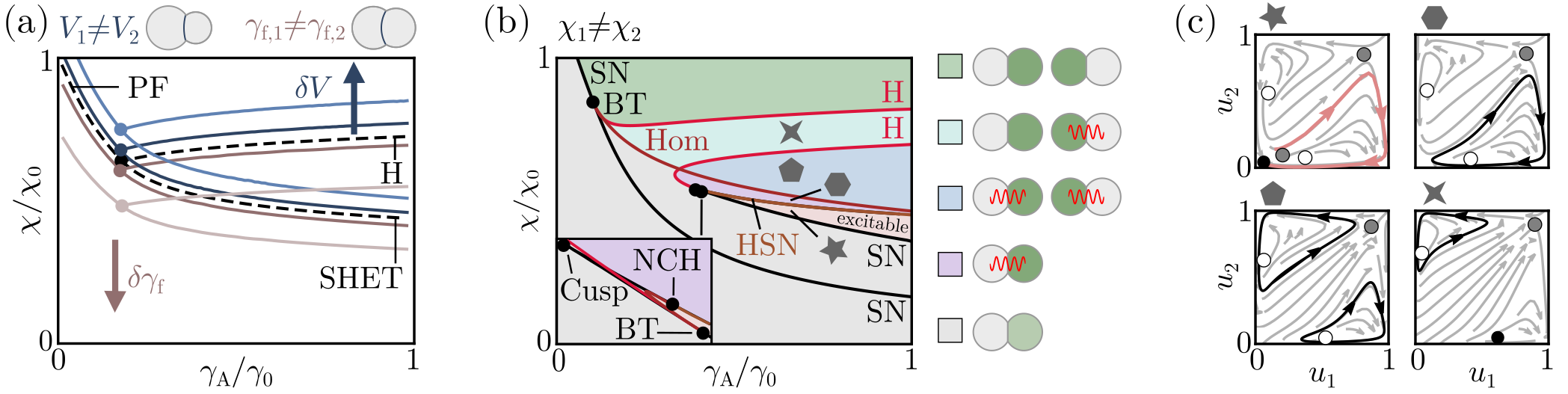
Figure 3: Nonlinear dynamics of asymmetric droplet pairs. (a) Differences in droplet volumes $\delta V/\bar{V}=\{0.25,0.5\}$ (blue) or outer tensions $\delta\gamma_{\rm{f}}/\bar{\gamma_{\rm{f}}}=\{0.25,0.5\}$ (brown) shift the SP point and associated bifurcation lines in the state diagram. (b) A difference in signal susceptibilities $\delta\chi/\bar{\chi}=0.05$ (i.e. $\chi_{1}/\chi_{2}\approx 1.1$) splits the SP point into a pair of Bogdanov-Takens bifurcation points (BT), a non-central homoclinic to saddle-node bifurcation (NCH) and associated bifurcation lines reconnect in a non-trivial fashion. Inlet shows the state diagram close to the second BT point ($\gamma_{\rm{A}}/\gamma_{0}\in[0.3896,0.403]$, $\chi/\chi_{0}\in[0.5388,0.5441]$). Note that NCH and BT are connected by a homoclinic (Hom). (HSN: Saddle-node homoclinic). (c) Phase portraits for parameter values marked with gray symbols in (b). (filled black circle: stable steady state, filled gray circle: saddle, open circle: unstable steady state, rose line: trajectory in the excitable regime, thick black line: limit cycle). Parameter values given in [28], Tab. 2.

Asymmetric droplets.—

The state-diagram structure associated with the SP point arises for identical droplets. While such state-space structures have been found and experimentally characterized for instance in optical cavities [45], most physical systems exhibit non-negligible variations in their properties. Differences in the properties of the interacting droplets change the state diagram shown in Fig. 2(a). For unequal droplet volumes $V_{1,2}=\bar{V}\pm\delta V$, symmetry-breaking and oscillatory dynamics emerge at a larger signaling susceptibility $\chi$ than in pairs of identical droplets, whereas a difference in the outer surface tensions $\gamma_{\rm{f},1,2}=\bar{\gamma_{\rm{f}}}\pm\delta\gamma_{\rm{f}}$ promotes symmetry-breaking and oscillations at lower susceptibilities due to partial internalization resulting in larger equilibrium contact areas [Fig. 3(a)].

Tension and volume asymmetry do not favour any droplet to reach a higher or lower internal state, because the signaling properties of each droplet remain unaffected, and thus the topology of the state space is preserved. In contrast, a difference in the signaling susceptibility $\chi_{1,2}=\bar{\chi}\pm\delta\chi$ splits the SP point into two Bogdanov-Takens (BT) codimension-2 points, and the SHET line into two homoclinics (Hom) and a saddle-node homoclinic (HSN) bifurcation line emerging from a non-central homoclinic to saddle-node (NCH) [Fig. 3(b)]. Accordingly, the limit cycle and the corresponding symmetry-broken state, in which the less susceptible droplet maintains the lower internal state, require lower values of $\chi$ and $\gamma_{\rm{A}}$ than the inverse symmetry-broken states. This allows for parameter regimes with single limit cycles [Fig. 3(c) hexagon] or coexistence with stable fixed points [Fig. 3(c) 4-pointed star]—contrary to the case of identical susceptibilities [Fig. 3(c) square and star]. Heterogeneous material properties can thus produce an even wider spectrum of dynamics.

Conclusions

Considering adaptive, interacting droplets, we obtained a tractable set of equations that reveal the rich physics arising in signal-processing active materials. In particular, we find that coupling between the geometry of droplet interfaces and the signals exchanged at these physical contacts enable robust symmetry-breaking, excitability, and self-sustained oscillations that can be tuned from sinusoidal to relaxation-like waveforms.

The critical points and associated phase-space structures we identify thus reveal how fundamental geometrical relations permit shape-adapting systems to produce a wide range of time-encoded outputs with few degrees of freedom. Indeed, dynamical features of signaling levels can program distinct cell fates[46, 47, 48], suggesting a role for shape-dependent feedback in the self-organisation of multicellular structures [49, 50].

Our findings will enable the discovery of new collective phenomena in active signal-processing materials, where mechanical feedback can drive spontaneous patterning and wave dynamics[51, 52, 53]. In particular, investigating fluctuation-induced effects in the excitable regimes will reveal when the large area deviations we report trigger topological transitions governing global rheological properties of materials such as tissues [54, 55]. Analysing these collective dynamics will uncover how geometry-dependent feedback produces novel modes of self-organisation in adaptive materials.

Acknowledgements

We gratefully acknowledge insightful discussions and valuable feedback from Florian Berger, Erwin Frey, Isabella Graf, Jeremy Gunawardena, Adrian Jacobo, Thomas Quail, Ulrich Schwarz, Alejandro Torres-Sánchez, Falko Ziebert and all members of the Erzberger Group. We acknowledge funding by the EMBL and TD was supported by a Joachim-Herz Add-on fellowship for interdisciplinary life science.

Supplementary Material

.1 Microscopic dynamics of signaling and adhesion

In the following, we consider a specific set of microscopic processes that can give rise to Eqs. (3)–(5). We derive the dynamics in the bulk $\Omega$ and at the surface $\Gamma$ of molecules controlling (i) adhesion at contact surfaces, and (ii) the exchange of chemical signals, motivated by the biochemical processes within and at the surface of biological cells. We consider continuity equations for the particle densities within the bulk $c$ and at the surface $m$ of the form [56]

$$\partial_{t}c =D_{\mathrm{c}}\nabla^{2}c+\mathcal{R}_{\mathrm{c}}$$ (6)

$$\partial_{t}m =D_{\mathrm{m}}\nabla^{2}m+\mathcal{R}_{\mathrm{m}}$$ (7)

in which we consider a diffusive flux with coefficients $D_{\rm{c}},D_{\rm{m}}$ in three and two dimensions respectively, and reaction terms $\mathcal{R}_{\rm{c}}$ and $\mathcal{R}_{\rm{m}}$. We do not consider convective flows or other active transport processes here. Bulk and surface densities are coupled by the boundary condition

$$-D_{\mathrm{c}}(\mathbf{n}\cdot\nabla)\left.c\right|_{\Gamma}=j$$ (8)

in which $j$ is the flux between bulk and surface and $\mathbf{n}$ is the normal vector to the surface pointing outwards. A simple form of this flux is given by [57, 43]

$$j=\left.k_{\mathrm{on}}c\right|_{\Gamma}-k_{\mathrm{off}}m$$ (9)

with $k_{\mathrm{on}}$ setting the rate with which molecules bind to the surface and $k_{\mathrm{off}}$ the rate with which they are released from the surface into the bulk. Note that a positive flux indicates that more molecules bind to the surface than are released into the bulk. Reactions in the bulk follow [58]

$$\mathcal{R}_{\mathrm{c}}=k_{\rm{p}}-k_{\rm{d}}c$$ (10)

with $k_{\mathrm{p}}$ describing an active production of molecules (e.g. due to protein translation in cells) and $k_{\mathrm{d}}$ their rate of decay (protein degradation). The bulk production of molecules drives the system out of thermodynamic equilibrium. For the surface reactions $\mathcal{R}_{\mathrm{m}}$, we consider different molecular processes governing adhesion and contact-based signaling, as specified in the following sections.

Averaging Eq. (6) over the bulk’s volume $V$ and using Eq. (8) and (10) yields the dynamic equation for the average bulk concentration $\langle c\rangle$

$$\frac{d\langle c\rangle}{dt}=k_{\mathrm{p}}-k_{\mathrm{d}}\langle c\rangle-\frac{1}{V}\int_{\Gamma}jdA.$$ (11)

We define the steady state average density in the absence of boundary flux as the reference density $c^{0}=k_{\mathrm{p}}/k_{\mathrm{d}}$, and defining $m^{0}=k_{\mathrm{on}}c^{0}/k_{\mathrm{off}}$ permits introducing normalized particle densities $c/c^{\mathrm{0}}$ and $m/m^{\mathrm{0}}$.

With diffusion timescale $\tau_{\mathrm{D}}=V^{2/3}/D_{\mathrm{c}}$ and reaction timescales $\tau_{\mathrm{R}}=1/k_{\mathrm{d}}$ and $\tau_{\mathrm{on}}=V^{1/3}/k_{\mathrm{on}}$, Eq. (6) and Eq. (8) with time rescaled in units of $\tau=t/\tau_{\rm{R}}$ read

$$\frac{\tau_{\mathrm{D}}}{\tau_{\rm{R}}}\frac{\partial_{\tau}c}{c^{0}} =V^{2/3}\nabla^{2}\frac{c}{c^{0}}+\frac{\tau_{\mathrm{D}}}{\tau_{\mathrm{R}}}\left(1-\frac{c}{c^{0}}\right),$$ (12)

$$\left(\mathbf{n}\cdot\nabla\right)\left.\frac{c}{c^{0}}\right|_{\Gamma} =\frac{\tau_{\mathrm{D}}}{\tau_{\mathrm{on}}V^{1/3}}\left(\frac{m}{m^{0}}-\frac{c}{c^{0}}\right).$$ (13)

In the the following, we consider the limit in which bulk diffusion is much faster than the reaction kinetics, i.e. $\tau_{\mathrm{D}}\ll\tau_{\mathrm{R}}$ and $\tau_{\mathrm{D}}\ll\tau_{\mathrm{on}}$. In this limit, the boundary condition Eq. (13) is reflective and Eq. 12 becomes a Laplace equation that is solved by a uniform concentration set by the solution of Eq. (11) (shadow limit [59]). Inside a cell, a typical diffusion constant for a monomeric protein is about $10\text{\,}{\mathrm{\SIUnitSymbolMicro m}}^{2}\text{\,}{\mathrm{s}}^{-1}$, i.e. it takes roughly 10 seconds for a protein to traverse a eukaryotic cell [60]. Coefficients of lateral diffusion on cellular membranes are variable and on the order of $0.011\text{\,}{\mathrm{\SIUnitSymbolMicro m}}^{2}\text{\,}{\mathrm{s}}^{-1}$ [43, 61]. Most biochemical reactions are catalyzed by enzymes and occur within less than a second [62], however transcription and translation, i.e. the synthesis of new proteins, and protein degradation take minutes to hours and can vary greatly between different proteins [63, 62].

The surface of an adherent droplet consists of two regions separated by a contact line: the domain of the contact interface $\Gamma_{\rm{c}}$ and the outer surface $\Gamma_{\rm{f}}$ [Fig. 1(a)]. At the outer surface, molecules can be exchanged with the bulk, but no adhesion or signaling dynamics occur within the surface, thus, the reaction term is $\left.\mathcal{R}_{m}\right|_{\Gamma_{\mathrm{f}}}=j$. We assume in the following that the contact line separating the two surfaces forms a diffusive barrier, i.e. that no molecules can diffuse laterally between the surfaces. This assumption substantially simplifies our calculations, and indeed diffusion barriers based on protein structures associated with the membrane, the lipid composition or extreme curvatures—as given at the contact line—have been found to impede diffusive transport on cellular membranes [64, 65]. The boundary conditions for the surface densities on the two domains then are

$$\left.(\mathbf{n}\cdot\nabla)m\right|_{\partial\Gamma_{\mathrm{f}}}=0$$ (14)

$$\left.(\mathbf{n}\cdot\nabla)m\right|_{\partial\Gamma_{\mathrm{c}}}=0$$ (15)

in which $\partial\Gamma_{\mathrm{f}},\partial\Gamma_{\mathrm{c}}$ denote the contact line. From Eqs. (7) follows at steady-state $\left.j\right|_{\Gamma_{\mathrm{f}}}=0$ and the uniform steady-state bulk concentration

$$c=\frac{k_{\mathrm{p}}}{k_{\mathrm{d}}}-\dfrac{1}{k_{\mathrm{d}}V}{\displaystyle\int_{\Gamma_{\mathrm{c}}}}jdA$$ (16)

only depends on processes in the bulk and at the contact site $\Gamma_{\mathrm{c}}$.

In the following sections, we analyse the distribution of molecules regulating signaling and adhesion in the limit of fast bulk diffusion. In particular, we introduce the reaction terms and corresponding boundary fluxes for the adhesion and signaling dynamics at the contact site and compute the steady-state bulk and surface densities that fulfill Eqs. (7), (16), and boundary condition $\eqref{eq:bc_Ac}$.

.2 Microscopic dynamics of adhesion

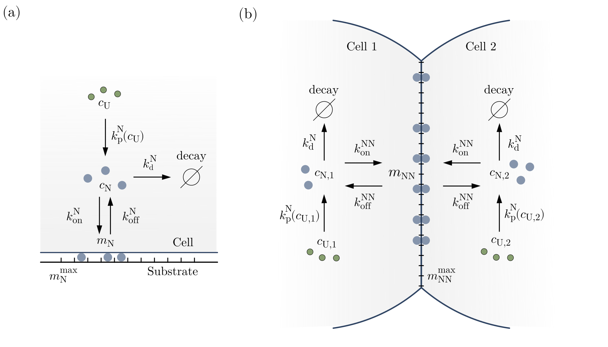
Figure 4: Schematic of adhesion dynamics for (a) a single adherent cell on a substrate and (b) adhesion complexes forming at a cell-cell interface. In the bulk, adhesion molecules (N) are produced (transcription + translation of genes) with a rate depending on the regulator concentration $c_{\mathrm{U}}$ and they decay over time with a constant rate. Adhesion molecules are exchanged between bulk and surface. At the cell-cell interface (b), two adhesion molecules—one from each cell—bind across the interface and form an adhesion complex. The maximum surface density of adhesion molecules is set by the number of available binding sites $m_{\mathrm{N}}^{\mathrm{max}}$ (a) and $m_{\mathrm{NN}}^{\mathrm{max}}$ (b), respectively. $c_{\mathrm{N}}$ indicates bulk concentrations, $m_{\mathrm{N}}$ (a) and $m_{\mathrm{NN}}$ (b) the surface densities of adhesion complexes and $k$ the various rate parameters.

We consider droplets containing adhesion molecules N with a bulk concentration $c_{\mathrm{N}}$, in contact either with an external substrate, or with another droplet. At a droplet-substrate interface, these molecules can adhere to the substrate with a surface density $m_{\mathrm{N}}$ [Fig. 4(a)], whereas at a droplet-droplet interface, molecules from the two droplets bind to each other and form complexes with surface concentration $m_{\mathrm{NN}}$ [Fig. 4(b)]. Cells for example produce integrin and cadherin molecules that form transmembrane complexes to adhere to external structures or other cells respectively [34].

We assume that the contact areas are given by the configuration minimizing the droplet surface energy (e.g. Eq. 1), i.e. that shape relaxation dynamics are fast compared to changes in adhesion density. For cells and cellular aggregates, the viscoelastic response to mechanical stresses comprises active and passive components and exhibits relaxation time scales spanning different orders of magnitudes [66]. For instance, when neutrophil cells are deformed by micropipette aspiration and subsequently expelled from the pipette, it takes around a minute for the cell to recover its spherical shape and shape evolution is well described by a Newtonian liquid drop with a constant cortical tension approaching its equilibrium configuration [67]. In contrast, protein production and degradation take place on a timescale of tens of minutes to several hours [63, 62].

.2.1 Adherent droplet on a substrate

We begin with a droplet that forms a physical contact with a solid substrate, to which adhesion molecules can bind [Fig. 4(a)]. A mass-action based reaction term for the surface concentration Eq. (7) reads

$$\mathcal{R}_{m_{\mathrm{N}}}=k_{\mathrm{on}}^{\mathrm{N}}(m_{\mathrm{N}}^{\mathrm{max}}-m_{\mathrm{N}})c_{\mathrm{N}}-k_{\mathrm{off}}^{\mathrm{N}}m_{\mathrm{N}}$$ (17)

with $m_{\mathrm{N}}^{\mathrm{max}}$ the density of available binding sites at the contact. The flux coupling bulk and contact surface is $j_{\mathrm{N}}=\mathcal{R}_{m_{\mathrm{N}}}$ and adhesion molecules bound to the substrate are fixed in place, i.e. $D_{m_{\mathrm{N}}}=0$ in Eq. (7). At steady-state, it follows from Eqs. (7), (16),(17) and boundary condition Eq. (15) that $j_{\mathrm{N}}=0$, $c_{\mathrm{N}}=k_{\mathrm{p}}^{\mathrm{N}}/k_{\mathrm{d}}^{\mathrm{N}}$, and

$$m_{\mathrm{N}}=\dfrac{k_{\mathrm{on}}^{\mathrm{N}}k_{\rm{p}}^{\mathrm{N}}}{k_{\mathrm{on}}^{\mathrm{N}}k_{\rm{p}}^{\mathrm{N}}+k_{\mathrm{off}}^{\mathrm{N}}k_{\rm{d}}^{\rm{N}}}m_{\mathrm{N}}^{\mathrm{max}}.$$ (18)

The same expression can also be derived from the grand canonical ensemble.

At steady-state, the flux coupling bulk and surface concentrations [Eq. (8)] vanishes and the surface can be considered to be in chemical and thermal equilibrium with a constant temperature $T$ and in contact with a bath of constant chemical potential $\mu=\mu(c_{\mathrm{N}})$ set by the steady-state bulk concentration. Note that the chemical potential is kept constant through a non-equilibrium process – the turnover of adhesion molecules. Each binding site at the interface is a two-state system: a binding site is either occupied or unoccupied. If $n$ is the number of occupied binding sites, $n^{\mathrm{max}}$ the total number of available binding sites at the surface and $\epsilon$ the binding energy, then the grand canonical partition sum for the whole surface reads

$$\Xi=\sum_{n=0}^{n^{\mathrm{max}}}\binom{n^{\mathrm{max}}}{n}e^{\beta n(\mu-\epsilon)}=\left(1+e^{\beta(\mu-\epsilon)}\right)^{n^{\mathrm{max}}}$$ (19)

with $\beta=(k_{\mathrm{B}}T)^{-1}$. The ensemble average of the number of occupied binding sites is

$$\langle n\rangle=\frac{1}{\beta}\frac{\partial\ln\Xi}{\partial\mu}=\frac{n^{\mathrm{max}}}{1+e^{\beta(\epsilon-\mu)}},$$ (20)

showing that the system follows Fermi-Dirac statistics. In the chemical equilibrium, the rates of binding and unbinding must be equal for each binding site. The binding rate of adhesion molecules is

$$k_{\mathrm{binding}}=k_{\mathrm{on}}^{\mathrm{N}}c_{\mathrm{N}}p_{\mathrm{uoc}}$$ (21)

with $p_{\mathrm{uoc}}=1/(1+e^{\beta(\mu-\epsilon)})$ the probability that a binding site is not occupied, while the unbinding rate is

$$k_{\mathrm{unbinding}}=k_{\mathrm{off}}^{\mathrm{N}}p_{\mathrm{oc}}$$ (22)

with $p_{\mathrm{oc}}=e^{\beta(\mu-\epsilon)}/(1+e^{\beta(\mu-\epsilon)})$ the probability that a binding site is occupied. From $k_{\mathrm{binding}}=k_{\mathrm{unbinding}}$ and Eqs. (21)–(22) follows

$$\frac{k_{\mathrm{off}}^{\mathrm{N}}}{k_{\mathrm{on}}^{\mathrm{N}}c_{\mathrm{N}}}=e^{\beta(\epsilon-\mu)}.$$ (23)

From $m_{\mathrm{N}}=\langle n\rangle/A_{\mathrm{c}}$ and $m_{\mathrm{N}}^{\mathrm{max}}=n^{\mathrm{max}}/A_{\mathrm{c}}$ together with Eq. (20) and $c_{\rm{N}}=k_{\rm{p}}^{\rm{N}}/k_{\rm{d}}^{\rm{N}}$ follows then Eq. (18).

Expansion in the dilute limit $k_{\mathrm{on}}^{\mathrm{N}}k_{\rm{p}}^{\rm{N}}/k_{\rm{d}}^{\rm{N}}\ll k_{\mathrm{off}}^{\mathrm{N}}$, i.e. where saturation effects do not play a role, yields

$$m_{\mathrm{N}}=\frac{k_{\mathrm{on}}^{\mathrm{N}}k_{\rm{p}}^{\mathrm{N}}}{k_{\mathrm{off}}^{\mathrm{N}}k_{\rm{d}}^{\rm{N}}}m_{\mathrm{N}}^{\mathrm{max}}+\mathcal{O}\left(\left(\frac{k_{\mathrm{on}}^{\mathrm{N}}k_{\rm{p}}^{\rm{N}}}{k_{\mathrm{off}}^{\mathrm{N}}k_{\rm{d}}^{\rm{N}}}\right)^{2}\right).$$ (24)

Given that each adhesion complex reduces the surface energy by $\epsilon$ [68], the surface tension at the contact site in this limit is

$$\gamma_{\mathrm{c}}=\gamma_{0}-\epsilon\frac{k_{\mathrm{on}}^{\mathrm{N}}k_{\rm{p}}^{\rm{N}}}{k_{\mathrm{off}}^{\mathrm{N}}k_{\rm{d}}^{\rm{N}}}m_{\mathrm{N}}^{\mathrm{max}},$$ (25)

with $\gamma_{0}$ the baseline tension containing all other contributions to the interfacial tension.

.2.2 Droplet-droplet adhesion

At contact surfaces between two droplets [Fig. 4(b)], adhesion molecules produced within the droplets can bind across the interface and form adhesion complexes with surface density $m_{\mathrm{NN}}$ [36]. Taking exclusion effects into account, adhesion complexes can only form at unoccupied sites on the interface. The density of unoccupied sites is $(m_{\mathrm{NN}}^{\mathrm{max}}-m_{\mathrm{NN}})$ with $m_{\mathrm{NN}}^{\mathrm{max}}$ the maximum possible density of adhesion complexes. The reaction term for the density of adhesion complexes is then

$$\mathcal{R}_{m_{\mathrm{NN}}}=k_{\mathrm{on}}^{\mathrm{NN}}(m_{\mathrm{NN}}^{\mathrm{max}}-m_{\mathrm{NN}})c_{\mathrm{N},1}c_{\mathrm{N},2}-k_{\mathrm{off}}^{\mathrm{NN}}m_{\mathrm{NN}}$$ (26)

with indices $\{1,2\}$ labeling the two droplets. The flux coupling bulk and surface densities is $j_{\mathrm{NN}}=\mathcal{R}_{m_{\mathrm{NN}}}$, and the tension at the droplet-droplet interface in the dilute limit $k_{\mathrm{on}}^{\mathrm{NN}}(k_{\rm{p}}^{\rm{N}}/k_{\rm{d}}^{\rm{N}})^{2}\ll k_{\mathrm{off}}^{\mathrm{NN}}$ is

$$\gamma_{\mathrm{c}}=\gamma_{0}-\epsilon\frac{k_{\mathrm{on}}^{\mathrm{NN}}}{k_{\mathrm{off}}^{\mathrm{NN}}}\left(\frac{k_{\rm{p}}^{\rm{N}}}{k_{\rm{d}}^{\rm{N}}}\right)^{2}m_{\mathrm{NN}}^{\mathrm{max}}.$$ (27)

Indeed, the force necessary to separate two adhesive cells has been shown to scale linearly with the squared total number of adhesion molecules [68, 69]. Note that in general the production or decay rates of adhesion molecules in the bulk [Eq. (10)] can differ between the two cells (Sec. .3.2). In particular, we consider in the following that the production rate of adhesion molecules $k_{\mathrm{p}}^{\mathrm{N}}$ depends on the cell-intrinsic signaling state (Secs. .3.1 and .3.2).

.3 Microscopic dynamics of biochemical signaling interactions at contact surfaces

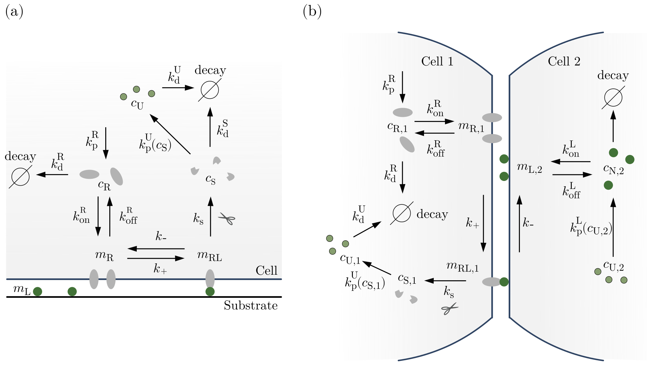
Figure 5: Schematic of signaling reaction kinetics for (a) a single adherent cell on a ligand-covered substrate and (b) signals exchanged at a cell-cell contact. Receptor (R, gray) and ligand (L, green) molecules bind across the interface and form receptor-ligand complexes (RL). In the single cell, ligands are substrate-bound whereas receptors are produced in the bulk and exchange with the surface. For cell pairs, we consider both receptors and ligands to bind and unbind from the cell-cell interface. Receptor-ligand complexes are cleaved irreversibly, which produces a signaling molecule (S, gray) that is released into the bulk. Regulator molecules (U, green) are produced with a rate that depends on the bulk concentration of signal molecules. The regulator U in turn determines the production rate of new ligands. In the single cell on the substrate (a), the ligand molecule is released upon the cleavage event and can bind a new receptor molecule. In the cell pair, we assume that the remaining part of the RL complex is degraded after the cleavage event. $c$ indicates bulk concentrations, $m$ surface densities and $k$ the various rate parameters.

Cells respond to molecular signals from the environment by changing their internal properties. Many cellular signals are transmitted via the binding of chemicals to receptor molecules located at the cell surface. These chemical events trigger internal processes, which result in changes to the molecular composition, spatial organisation, and corresponding functions of cells [11]. Signaling processes are relevant for example in chemotactic bacteria [70, 9, 71, 72], sensory neurons of the olfactory system [73], immune cell activation by pathogenic molecules [74] or stem cells responding to differentiation cues [75].

Signals can arise at physical contacts with surrounding structures (e.g. the extracellular matrix) or neighboring cells such that the geometry of contacts in a given system determines the possible signaling partners and affects the signaling outcome [14, 76, 44, 43]. For instance, in the Notch signaling pathway, signaling relies on direct interactions between membrane-bound receptor and ligand molecules [Fig. 5]. Their interaction triggers a series of proteolytic cleavage events of the receptor at the end of which the intracellular receptor domain dissociates from the surface and translocates into the nucleus, where it regulates the expression of target genes [15]. Following the example of the Notch pathway, we consider the reaction-diffusion dynamics of receptors (R), ligands (L), and receptor-ligand complexes (RL) at a signaling interface, and derive how the bulk concentration of signal molecules (S) responds to these interactions at the boundary [Fig. 5]. Similar to how the Notch intracellular domain regulates gene expression, we consider that the concentration of signal molecules in turn determines the production rate of a regulator molecule (U) in the bulk (e.g. a cellular transcription factor) that controls the production rates of adhesion and signaling molecules. Given that the regulation of transcription, translation and the turnover of proteins requires tens of minutes to hours and can vary greatly between different protein species [62, 77], we assume that the timescale associated with the regulator turnover $\tau_{\mathrm{u}}$ dominates the feedback dynamics. On this timescale, we assume that bulk and surface concentrations relax to their steady state solutions, and that the shape takes on the corresponding equilibrium configuration. In cells, concentration and shape dynamics are indeed typically at least an order of magnitude faster – set by diffusive, biochemical, and viscoelastic timescales which are on the order of seconds to minutes [66, 43, 61, 62].

.3.1 A cell on a signal transmitting substrate

We begin with a single cell in contact with a solid substrate that is covered with ligands at a fixed uniform density $m_{\mathrm{L}}^{\mathrm{max}}$, similar to experimental systems developed for the Notch pathway in in vitro assays [78] [Fig. 5(a)]. The cell contains receptor molecules, signaling molecules, and regulator molecules with bulk concentrations $c_{\mathrm{R}},c_{\mathrm{S}},$ and $c_{\mathrm{U}}$ respectively, whose dynamics are coupled via the reactions at the contact surface. We do not explicitly consider a bulk concentration of ligands, because the substrate has no receptor molecules to bind to—the cell is only receiving, but not sending signals. To describe the signaling dynamics at the surface, we use Eq. (7) for the surface densities of receptors $m_{\rm{R}}$, substrate-bound ligands $m_{\rm{L}}$ and receptor-ligand complexes $m_{\rm{RL}}$ with the reaction terms adapted from Khait et al. (2016) [43]

$$\mathcal{R}_{m_{\mathrm{R}}} =k_{\rm{on}}^{\rm{R}}c_{\rm{R}}-(k_{\rm{off}}^{\rm{R}}+k_{+}m_{\rm{L}})m_{\rm{R}}+k_{-}m_{\rm{RL}},$$ (28)

$$\mathcal{R}_{m_{\mathrm{L}}} =(k_{-}+k_{\rm{s}})m_{\rm{RL}}-k_{+}m_{\rm{L}}m_{\rm{R}},$$ (29)

$$\mathcal{R}_{m_{\mathrm{RL}}} =k_{+}m_{\rm{L}}m_{\rm{R}}-(k_{-}+k_{\rm{s}})m_{\rm{RL}},$$ (30)

which are explained in the following [Fig. 5(a)]. Receptors are recruited to the surface with a rate set by $k^{\rm{R}}_{\rm{on}}$ (exocytosis) and they are removed from the surface with rate $k^{\rm{R}}_{\rm{off}}$ (endocytosis). Receptors at the contact surface bind ligands at a rate determined by $k_{+}$ to form receptor-ligand complexes, which unbind with rate $k_{-}$. Receptor-ligand complexes undergo an irreversible enzymatic cleavage with rate $k_{\rm{s}}$ upon which a fragment of the bound receptor molecule is released into the bulk and acts as a signaling molecule (S), the remaining part is degraded, and the ligand is released within the surface where it can bind to a new receptor molecule.

The bulk concentration $c_{\mathrm{S}}$ of signaling molecules controls the bulk production rate $k_{\mathrm{p}}^{\mathrm{U}}(c_{\mathrm{S}})$ of the regulator U [see below, Eq. (41)]. The bulk concentrations of receptors $c_{\mathrm{R}}$ and signaling molecules $c_{\mathrm{S}}$ are coupled to the signaling dynamics at the contact via Eq. (16).

We consider the ligands on the substrate to be bound and fixed in place, such that $D_{m_{\mathrm{L}}}=0,D_{m_{\mathrm{RL}}}=0$ in Eq. (7). The density of unbound ligands is the difference between the total density of ligands covering the substrate and the density of receptor-ligand complexes $m_{\mathrm{L}}=m_{\mathrm{L}}^{\mathrm{max}}-m_{\mathrm{RL}}$. Equations (7) and (30) together with this relation permit expressing the steady-state concentration of receptor-ligand complexes in terms of the steady-state receptor concentration as

$$m_{\mathrm{RL}} =\frac{m_{\mathrm{R}}}{m_{\mathrm{R}}+\dfrac{k_{\mathrm{s}}+k_{-}}{k_{+}}}m_{\mathrm{L}}^{\mathrm{max}}.$$ (31)

Given Eqs. (7), (28) and (31), the steady-state relation for the distribution of receptors reads

$$0=D_{m_{\mathrm{R}}}\nabla^{2}m_{\rm{R}}+k_{\rm{on}}^{\rm{R}}c_{\mathrm{R}}-k_{\rm{off}}^{\rm{R}}m_{\rm{R}}-\frac{k_{s}k_{+}m_{\mathrm{R}}}{k_{+}m_{\mathrm{R}}+k_{\mathrm{s}}+k_{-}}m_{\mathrm{L}}^{\mathrm{max}}.$$ (32)

In the limit where the rate of receptors binding to ligands on the substrate is large compared to the transport of receptors from the surface into the bulk, i.e.

$$k_{+}m_{\mathrm{L}}^{\mathrm{max}}\gg k_{\mathrm{off}}^{\mathrm{R}},$$ (33)

solutions of Eq. (32) are uniform and follow

$$m_{\rm{R}}=\frac{k_{\rm{on}}^{\rm{R}}c_{\rm{R}}(k_{-}+k_{\rm{s}})}{k_{+}(k_{\rm{s}}m_{\rm{L}}^{\rm{max}}-k_{\rm{on}}^{\rm{R}}c_{\rm{R}})},$$ (34)

under boundary condition Eq. (15). The bulk and surface densities of receptors are coupled via the flux [Eq. (16)]

$$j_{\mathrm{R}} =k_{\mathrm{on}}^{\mathrm{R}}c_{\mathrm{R}}-k_{\mathrm{off}}^{\mathrm{R}}m_{\mathrm{R}}.$$ (35)

Using Eq. (34) and assuming (33), the flux can be approximated as $j_{\rm{R}}=k_{\rm{on}}^{\rm{R}}c_{\rm{R}}$ and the steady-state bulk and surface densities of receptors that follow from Eqs. (16) and (34) are given by

$$c_{\rm{R}} =\frac{k_{\rm{p}}^{\rm{R}}V}{k_{\rm{d}}^{\rm{R}}V+k_{\rm{on}}^{\rm{R}}A_{\rm{c}}},$$ (36)

$$m_{\rm{R}} =\frac{k_{\rm{on}}^{\rm{R}}k_{\rm{p}}^{\rm{R}}(k_{-}+k_{\rm{s}})V}{k_{+}[k_{\rm{s}}m_{\rm{L}}^{\rm{max}}(k_{\rm{on}}^{\rm{R}}A_{\rm{c}}+k_{\rm{d}}^{\rm{R}}V)-k_{\rm{on}}^{\rm{R}}k_{\rm{p}}^{\rm{R}}V]}.$$ (37)

For Notch receptors, reported values are $k_{+}=$0.167\text{\,}{\mathrm{\SIUnitSymbolMicro m}}^{2}\text{\,}{\mathrm{s}}^{-1}$$ and $k_{\mathrm{off}}^{\rm{R}}=$0.02\text{\,}{\mathrm{s}}^{-1}$$ [43] [Tab.] and Notch activation assays with cells on ligand-coated substrates are performed with surface densities of up to $m_{\rm{L}}^{\rm{max}}\approx${10}^{5}\text{\,}{\mathrm{\SIUnitSymbolMicro m}}^{-2}$$ [78], which justifies limit (33) and allows to neglect the $k_{\rm{off}}^{\rm{R}}$-term in Eq. (32). Importantly, $m_{\rm{R}}$ and $c_{\rm{R}}$ have upper bounds: in the absence of ligands ($m_{\mathrm{L}}^{\mathrm{max}}=0$), the steady-state receptor density is uniform at $m_{\rm{R}}^{0}=k_{\mathrm{on}}^{\mathrm{R}}c_{\mathrm{R}}^{0}/k_{\mathrm{off}}^{\mathrm{R}}$ with bulk concentration $c_{\rm{R}}^{0}=k_{\mathrm{p}}^{\mathrm{R}}/k_{\mathrm{d}}^{\mathrm{R}}$. Because receptors are removed upon receptor-ligand binding and subsequent cleavage, $m_{\rm{R}}^{0}$ and $c_{\mathrm{R}}^{0}$ are upper bounds to the steady-state concentrations. If we estimate the term in brackets of Eq. (32) using $m_{\rm{R}}=m_{\rm{R}}^{0}$ and typical parameter values as listed in Tab. 1, neglecting $k_{\rm{off}}^{\rm{R}}$ is valid if $m_{\rm{L}}^{\rm{max}}\gg$10\text{\,}{\mathrm{\SIUnitSymbolMicro m}}^{-2}$$.

Given Eqs. (31) and (37), the steady-state density of receptor-ligand complexes is

$$m_{\rm{RL}}=\frac{k_{\rm{on}}^{\rm{R}}k_{\rm{p}}^{\rm{R}}V}{k_{\rm{s}}(k_{\rm{on}}^{\rm{R}}A_{\rm{c}}+k_{\rm{d}}^{\rm{R}}V)}.$$ (38)

The bulk concentration of signaling molecules follows Eq. (16), without a bulk production term ($k_{\mathrm{p}}^{\mathrm{S}}=0$) and with flux $j_{\mathrm{S}}=-k_{\mathrm{s}}m_{\mathrm{RL}}$, arising from the cleavage of receptor-ligand molecules at the surface. The steady-state bulk concentration is given by

$$c_{\mathrm{S}}=\frac{k_{\rm{on}}^{\rm{R}}k_{\rm{p}}^{\rm{R}}A_{\mathrm{c}}}{k_{\rm{d}}^{\rm{S}}(k_{\rm{on}}^{\rm{R}}A_{\rm{c}}+k_{\rm{d}}^{\rm{R}}V)}.$$ (39)

In general, the concentration of signaling molecules depends non-linearly on the size of the contact area. When the number of receptors that are recruited to the surface and lost in the signaling process is small compared to the turnover of molecules in the bulk, we can expand the bulk concentration of signal molecules

$$c_{\mathrm{S}}=\frac{k_{\rm{p}}^{\rm{R}}k_{\rm{on}}^{\rm{R}}A_{\rm{c}}}{k_{\rm{d}}^{\rm{S}}k_{\rm{d}}^{\rm{R}}V}+\mathcal{O}\left(\left(\frac{k_{\mathrm{on}}^{\mathrm{R}}A_{\mathrm{c}}}{k_{\mathrm{d}}^{\mathrm{R}}V}\right)^{2}\right).$$ (40)

In in vitro experiments, a roughly linear relation between Notch response and contact area was measured also for large contact areas [43].

The production of regulator molecules U in the bulk depends on the steady-state concentration of signal molecules $k_{\mathrm{p}}^{\mathrm{U}}(c_{\mathrm{s}})$ —the more signal molecules are present, the more regulator molecules are produced. The regulation of genes and the synthesis of new proteins involve multiple steps and molecular species, which leads to the presence of nonlinear effects like cooperative binding and multimerization, commonly captured using Hill-functions [79]. Similar to previous studies modeling canonical Notch signaling [16, 42, 30, 41], we therefore assume that steady-state solutions of $c_{\mathrm{U}}$ are bounded within a concentration range $c_{\mathrm{U}}^{\mathrm{min}}\leq c_{\mathrm{U}}\leq c_{\mathrm{U}}^{\mathrm{max}}$ [Fig. 6] and we consider a nonlinear production rate with Hill coefficient $h$

$$k_{\mathrm{p}}^{\mathrm{U}}(c_{\mathrm{S}})=\frac{1}{\tau_{\mathrm{u}}}\left(c_{\mathrm{U}}^{\mathrm{min}}+\frac{(c_{\mathrm{U}}^{\mathrm{max}}-c_{\mathrm{U}}^{\mathrm{min}})}{1+\left(\frac{c_{\mathrm{S}}^{\mathrm{crit}}}{c_{\mathrm{S}}}\right)^{h}}\right)$$ (41)

in which $\tau_{\mathrm{u}}=1/k_{\mathrm{d}}^{\mathrm{U}}$ is the characteristic time scale on which $c_{\mathrm{U}}$ is changing, and $c_{\mathrm{S}}^{\mathrm{crit}}$ is the critical concentration at the inflection point [Fig. 6].

The normalized signal $s=c_{\mathrm{S}}/c_{\mathrm{S}}^{\mathrm{crit}}$ can be written using Eq. (39) as

$$s=\chi\frac{A_{\mathrm{c}}}{A_{0}},$$ (42)

in which we introduced the signal susceptibility

$$\chi=\frac{k_{\mathrm{p}}^{\rm{R}}k_{\rm{on}}^{\rm{R}}}{c_{\mathrm{S}}^{\mathrm{crit}}k_{\mathrm{d}}^{\mathrm{S}}k_{\rm{d}}^{\rm{R}}V}A_{\mathrm{0}}.$$ (43)

using the definition of the volume-dependent reference area $A_{0}=(3V/2)^{2/3}\pi^{1/3}$. The volume-dependence of the susceptibility arises because the degradation of molecules in the bulk scales with the volume, and due to the reference area $A_{0}$, yielding a scaling of $\chi\propto V^{-1/3}$. However, in cells where protein degradation does not increase with the cell volume, the signal susceptibility might increase with volume. Interestingly, the signal susceptibility is independent of the cleavage rate $k_{\rm{s}}$. A common experimental perturbation to Notch signaling is the pharmacological inhibition of the enzyme cleaving the receptor-ligand complexes (treatment of cells with $\gamma$-secretase inhibitors) [80]. Our result suggests that the signal susceptibility and thus the steady-state concentration of signaling molecules is independent of $k_{\rm{s}}$ unless cleavage is completely prevented. We can estimate the order of magnitude of the susceptibility using $k_{\rm{on}}^{\rm{R}}k_{\rm{p}}^{\rm{R}}/k_{\rm{d}}^{\rm{R}}=$2\text{\,}{\mathrm{\SIUnitSymbolMicro m}}^{-2}\text{\,}{\mathrm{s}}^{-1}$$ [43], $V=$500\text{\,}{\mathrm{\SIUnitSymbolMicro m}}^{3}$$, $k_{\rm{d}}^{\rm{S}}=$5\text{\times}{10}^{-3}\text{\,}{\mathrm{min}}^{-1}$$ [81, 82] and $c_{\rm{S}}^{\rm{crit}}=1000/V$ [83] yielding $\chi\sim 3000$.

The uniform bulk concentration $c_{\mathrm{U}}$ evolves on the slowest timescale of the system, the regulatory time scale $\tau_{\mathrm{u}}$, according to Eq. (11), in which $j_{\mathrm{U}}=0$ because regulator molecules do not bind to the surface. The saturating response to the received signal [Eq. (41)] permits introducing a dimensionless signaling state variable

$$u:=\frac{c_{\mathrm{U}}-c_{\mathrm{U}}^{\mathrm{min}}}{c_{\mathrm{U}}^{\mathrm{max}}-c_{\mathrm{U}}^{\mathrm{min}}},$$ (44)

normalized to the response range such that $u\in[0,1]$. Eqs. (11), (41), (42), and (44) lead to the following dynamical equation for the signaling state

$$\tau_{\mathrm{u}}\frac{du}{dt}=\sigma(s)-u,$$ (45)

with sigmoidal response function

$$\sigma(s)=\frac{s^{h}}{1+s^{h}}.$$ (46)

as given in the main text.

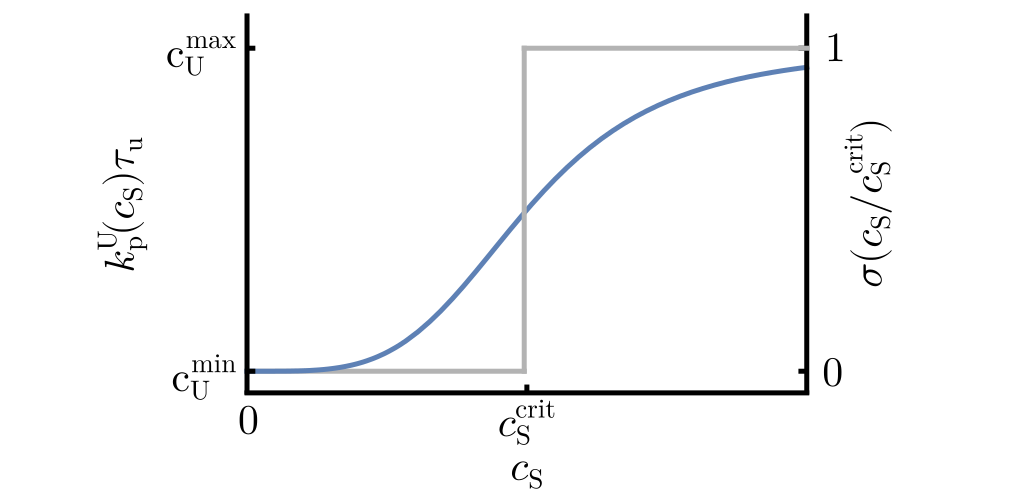
Figure 6: Sigmoid signal response function Eq. (41) describing the production rate of regulator molecules $k_{\mathrm{p}}^{\mathrm{U}}$ on time scale $\tau_{\mathrm{u}}$ within the concentration range $c_{\mathrm{U}}^{\mathrm{min}}\leq c_{\mathrm{U}}\leq c_{\mathrm{U}}^{\mathrm{max}}$ depending on the signal molecule concentration $c_{\mathrm{S}}$. For the temporal dynamics of the normalized signaling state variable $u$ [Eq. (44)], this can be mapped to a corresponding response function $\sigma$ [Eq. (46)] scaling between 0 and 1 [see also Fig. 1(c)]. Plot shown for $h=4$ (blue) and in the limit $h\rightarrow\infty$ (gray), where the response is a step function of $c_{\rm{S}}$.

Signal-dependent active mechanics.—

In many biological systems, for instance mechanosensory epithelia [84, 85, 16], adhesion molecules are expressed downstream of contact-based signals. Accordingly, we consider that the production rate of adhesion molecules $k_{\mathrm{p}}^{\mathrm{N}}(c_{\mathrm{U}})$ is a monotonously increasing function of the regulator concentration. As stated above, such a function is generally expected to be nonlinear, e.g. due to cooperativity between molecules involved in protein synthesis [79]. In the following, we assume that $k_{\mathrm{p}}^{\mathrm{N}}$ vanishes for $c_{\mathrm{U}}\leq c_{\mathrm{U}}^{\mathrm{min}}$, i.e. no adhesion molecules are produced when the regulator concentration drops below $c_{\mathrm{U}}^{\mathrm{min}}$, and we linearize $k_{\mathrm{p}}^{\mathrm{N}}$ around $c_{\mathrm{U}}^{\mathrm{min}}$

$$k_{\mathrm{p}}^{\mathrm{N}}(c_{\mathrm{U}})=\left.\frac{dk_{\mathrm{p}}^{\mathrm{N}}}{dc_{\mathrm{U}}}\right\rvert_{c_{\mathrm{U}}^{\mathrm{min}}}(c_{\mathrm{U}}-c_{\mathrm{U}}^{\mathrm{min}})+\mathcal{O}\left((c_{\mathrm{U}}-c_{\mathrm{U}}^{\mathrm{min}})^{2}\right).$$ (47)

With Eq. (44) the surface tension at the contact site [Eq. (25)] can then be written as

$$\gamma_{\mathrm{c}}=\gamma_{0}-\gamma_{\mathrm{A}}u$$ (48)

with the adaptive adhesion coefficient

$$\gamma_{\mathrm{A}}=\epsilon\frac{k_{\mathrm{on}}^{\mathrm{N}}(c_{\mathrm{U}}^{\mathrm{max}}-c_{\mathrm{U}}^{\mathrm{min}})}{k_{\mathrm{off}}^{\mathrm{N}}k_{\mathrm{d}}^{\mathrm{N}}}\left.\frac{dk_{\mathrm{p}}^{\mathrm{N}}}{dc_{\mathrm{U}}}\right\rvert_{c_{\mathrm{U}}^{\mathrm{min}}}m_{\mathrm{L}}^{\mathrm{max}}.$$ (49)

We can estimate the magnitude of $\gamma_{\rm{A}}$ for a cell that detaches if $u=0$ (i.e. $A_{\rm{c}}=0$ and $\gamma_{\rm{c}}=\gamma_{\rm{m}}$+$\gamma_{\rm{f}}$) and acquires a half-sphere shape if $u=1$ (i.e. $A_{\rm{c}}=A_{0}$ and $\gamma_{\rm{c}}=\gamma_{\rm{m}}$), in which case $\gamma_{\rm{A}}=\gamma_{\rm{f}}$. In cells, $\gamma_{\rm{f}}$ is typically on the order of $1\text{\,}\mathrm{mN}\text{\,}{\mathrm{m}}^{-1}$ [86].

Feedback between contact-based signaling and adaptive mechanics creates bistability.—

Equations (42) and (48) describe respectively how transmitted signals depend on the area of the cell-substrate interface, and how the interfacial tension in turn depends on the signaling state. Given that cell shape dynamics are fast compared to the signaling timescale $\tau_{\rm{u}}$, the area is determined quasi-instantaneously by the conjugate interfacial tension $\gamma_{\rm{c}}$.

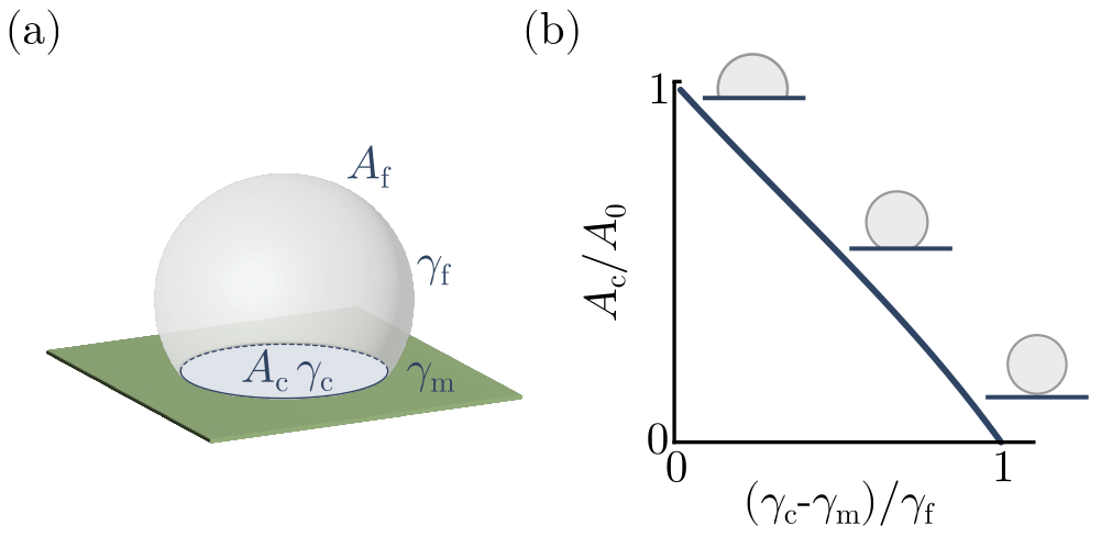
Figure 7: a) Schematic of a spherical-cap-shaped droplet attached to a substrate. The droplet has an outer surface area $A_{\mathrm{f}}$ and forms a contact of size $A_{\mathrm{c}}$ with the substrate. $\gamma_{\mathrm{c}}$ and $\gamma_{\mathrm{f}}$ are the area-associated surface tensions and $\gamma_{\mathrm{m}}$ the interfacial tension between substrate and surrounding medium. b) Normalized contact area $A_{\mathrm{c}}/A_{0}$ at minimal surface energy (Eq. 51) as a function of the surface tension ratio $(\gamma_{\mathrm{c}}-\gamma_{\mathrm{m}})/\gamma_{\mathrm{f}}$.

We consider the equilibrium configuration that minimizes the surface energy of an incompressible droplet in contact with a solid substrate

$$E=\int_{A_{\mathrm{c}}}(\gamma_{\mathrm{c}}-\gamma_{\mathrm{m}})dA+\int_{A_{\mathrm{f}}}\gamma_{\mathrm{f}}dA+E_{0}$$ (50)

with $\gamma_{\mathrm{m}}$ the energy per area between the substrate and the surrounding medium and $E_{0}$ depending on the total size of the substrate [Fig. 7(a)]. The surface energy is minimal when the droplet takes the shape of a spherical cap with normalized contact area [Fig. 7(b)]

$$\frac{A_{\mathrm{c}}}{A_{0}}=\left[1-\left(\dfrac{\gamma_{\mathrm{c}}-\gamma_{\mathrm{m}}}{\gamma_{\mathrm{f}}}\right)^{2}\right]\left[\frac{2}{(2-\dfrac{\gamma_{\mathrm{c}}-\gamma_{\mathrm{m}}}{\gamma_{\mathrm{f}}})(1+\dfrac{\gamma_{\mathrm{c}}-\gamma_{\mathrm{m}}}{\gamma_{\mathrm{f}}})^{2}}\right]^{2/3}.$$ (51)

Equations (42), (45), (48), and (51) describe the dynamics of the signaling state $u$ and contact area $A_{\mathrm{c}}$ of the adherent cell. We use a combination of linear stability analysis and simulations to study the steady-state solutions of this system. For different parameter combinations of $\chi$ and $\gamma_{\mathrm{A}}$, either one or two stable steady-state solutions $u^{*}$ are found [Fig.(2)(c)]. In particular, a bistable regime appears above a critical value of the adaptive tension $\gamma_{A}^{\mathrm{cusp}}$, bounded by two saddle-node bifurcation lines (SN), which converge in a cusp node [Fig.(2)(c)]. For $\gamma_{\rm{A}}>\gamma_{A}^{\mathrm{cusp}}$ and small $\chi$, the only stable solution is a configuration with small contact area $A_{\mathrm{c}}$, correspondingly weak signal transmission and a low signaling state $u$. For $\chi>\chi_{\rm{SN1}}$ —above the lower SN line— a second stable configuration appears with a large contact area $A_{\mathrm{c}}$, which permits a stronger signaling interaction with the substrate and a larger signaling state $u$ [Fig.(2)(c), inset]. This latter configuration is accessible only when the positive feedback between signaling and adaptive mechanics is sufficiently strong. The same bistability between a small and a large contact area configurations is also the basis for the shape oscillations we report in pairs of adaptive droplets [Fig. 2 (d)].

In the limit $h\rightarrow\infty$ [Eq. (46)], i.e. when the production of regulator molecules responds to signals in a step-wise manner [Fig. 6], one can derive a simple relation between $\chi$ and $\gamma_{A}$ for the two saddle-node lines. In general in this limit, the only possible stable steady-state solutions of Eq. (45) are $u^{*}\in\{0;1\}$ and the corresponding surface tensions at the contact site [Eq. (48)] are $\gamma_{c}\in\{\gamma_{0};\gamma_{0}-\gamma_{A}\}$. For small values of $\chi$, signaling is weak and the only stable steady-state is $u^{*}=0$ with a small contact area set by $\gamma_{c}=\gamma_{0}$. The second stable steady-state $u^{*}=1$ appears for

$$s(\left.A_{\mathrm{c}}\right|_{\gamma_{0}-\gamma_{A}})\geq 1.$$ (52)

For

$$s(\left.A_{\mathrm{c}}\right|_{\gamma_{0}})>1,$$ (53)

the configuration with small contact area and $u=0$ is no longer a steady-state solution and $u^{*}=1$ remains the only stable steady-state. From conditions  (52)–(53) together with (42) follows that the critical susceptibilities at the saddle-node lines delineating the bistable regime are given by

$$\chi_{1}=\frac{A_{0}}{\left.A_{\mathrm{c}}\right|_{\gamma_{\mathrm{c}}=\gamma_{0}-\gamma_{\mathrm{A}}}}$$ (54)

and

$$\chi_{2}=\frac{A_{0}}{\left.A_{\mathrm{c}}\right|_{\gamma_{\mathrm{c}}=\gamma_{0}}}.$$ (55)

with $\chi_{1}$ describing the lower and $\chi_{2}$ the upper saddle-node line [Fig. 8(a)]. Note that in the discussed limit the upper saddle-node bifurcation line ($\chi_{2}$) is independent of the adaptive adhesion coefficient $\gamma_{\mathrm{A}}$ [Fig. 8(a)]. In general, the saddle-node bifurcation lines and therefore the size of the bistable regime depend on the baseline tension $\gamma_{0}$. Fig. 8(b) shows for the discussed limit how the size of the bistable regime increases with the baseline tension.

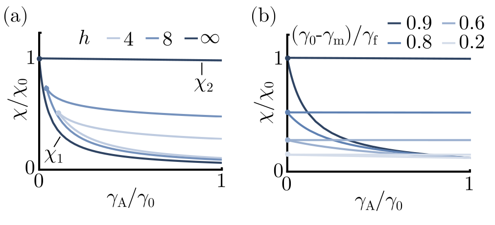
Figure 8: The state diagram of a single adherent droplet on a signal-transmitting solid substrate depends on (a) the Hill coefficient $h$ in the nonlinear response function [Eq.(46)] and (b) the baseline tension $\gamma_{0}$. Lines are saddle-node bifurcation lines that converge in a cusp node bifurcation (filled circles) and that encompass a bistable regime [compare to Fig. 2 (b)]. The reference susceptibilities are (a) $\chi_{0}=A_{0}/\left.A_{\mathrm{c}}\right|_{h=\infty}$ and (b) $\chi_{0}=A_{0}/\left.A_{\mathrm{c}}\right|_{(\gamma_{0}-\gamma_{m})/\gamma_{f}=0.9}$. (a) $(\gamma_{0}-\gamma_{m})/\gamma_{f}=0.95$, (b) $h=\infty$.

.3.2 Signaling in pairs of cells

In this section, we consider contact-dependent signals exchanged between two cells indexed with $i,j\in\{1,2\}$ that share an interface [Fig. 5(b)]. In addition to containing signaling and regulator molecules, each cell produces receptors as well as ligands, which exchange between bulk and surface – ligands are not substrate-bound with fixed positions as we considered in the preceding part. The receptors on the surface of cell $i$ bind to the ligands on the surface of the other cell $j$ and vice versa, producing respectively oriented receptor-ligand complexes. Upon cleavage they release signal molecules into the receptor-carrying cell $i$. Contrary to the way we treated substrate-bound ligands in the preceding section, ligands at the droplet interface are not released after cleavage of the receptor-ligand complexes, but are degraded together with the remaining receptor fragment instead [87]. While some literature suggests that ligands can also be recycled after a signaling event or enter alternative signaling pathways [88, 89], we here consider that receptors and ligands are always degraded after cleavage. Signaling molecules control the production of regulator molecules as before, which feed back onto the production terms. In line with the typical molecular mechanisms in Notch signaling, we consider an active regulation of ligand production [90]. As explained in Sec. .1, the steady-state bulk concentrations of receptor, ligand, signaling, and regulator molecules are uniform within each cell with a value set by the flux balance condition [Eq. (16)]. To capture the reaction-diffusion dynamics at the interface, we study Eq. (7) for receptors, ligands, and complexes using the reaction terms [43]

$$\mathcal{R}_{\mathrm{R}} =k_{\mathrm{on}}^{\mathrm{R}}c_{\mathrm{R},i}-(k_{\mathrm{off}}^{\mathrm{R}}+k_{+}m_{\mathrm{L},j})m_{\mathrm{R},i}+k_{-}m_{\mathrm{RL},i}$$ (56)

$$\mathcal{R}_{\mathrm{L}} =k_{\mathrm{on}}^{L}c_{\mathrm{L},j}-(k_{\mathrm{off}}^{\mathrm{L}}+k_{+}m_{\mathrm{R},i})m_{\mathrm{L},j}+k_{-}m_{\mathrm{RL},i}$$ (57)

$$\mathcal{R}_{\mathrm{RL}} =k_{+}m_{\mathrm{R},i}m_{\mathrm{L},j}-(k_{-}+k_{\mathrm{s}})m_{\mathrm{RL},i},$$ (58)

with rate constants as described in Sec. .3.1. Under boundary condition Eq. (15), steady-state solutions of Eq. (7) for the densities of receptors, ligands and receptor-ligand complexes with the reaction terms Eqs. (56)-(58) are uniform and follow the relations

$$m_{\mathrm{R},i} =\frac{k_{\rm{on}}^{\rm{R}}c_{\mathrm{R},i}(k_{\rm{s}}+k_{-})}{k_{\rm{off}}^{\rm{R}}(k_{\rm{s}}+k_{-})+k_{+}k_{\rm{s}}m_{\mathrm{L},j}},$$ (59)

$$m_{\mathrm{L},j} =\frac{k_{\rm{on}}^{\rm{L}}c_{\mathrm{L},j}(k_{\rm{s}}+k_{-})}{k_{\rm{off}}^{\rm{L}}(k_{\rm{s}}+k_{-})+k_{+}k_{\rm{s}}m_{\mathrm{R},i}}.$$ (60)

Ligand molecules are only produced in the bulk, but not at the surface, thus, the steady-state concentrations of bulk and surface densities have the upper limits $c_{\rm{L}}^{\mathrm{0}}=k_{\mathrm{p}}^{\rm{L}}/k_{\mathrm{d}}^{\rm{L}}$ and $m_{\rm{L}}^{\mathrm{0}}=k_{\mathrm{on}}^{\rm{L}}c^{\mathrm{0}}/k_{\mathrm{off}}^{\rm{L}}$. Together with Eqs. (59) and (16) for the receptor bulk concentration, one can define a lower limit for the surface density of receptors

$$m_{\rm{R}}^{\rm{min}}=\frac{k_{\rm{on}}^{\rm{R}}k_{\rm{off}}^{\rm{L}}(k_{-}+k_{\rm{s}})k_{\rm{p}}^{\rm{R}}k_{\rm{d}}^{\rm{L}}V}{k_{\rm{on}}^{\rm{L}}k_{+}k_{\rm{s}}k_{\rm{p}}^{\rm{L}}(k_{\rm{on}}^{\rm{R}}A_{\rm{c}}+k_{\rm{d}}^{\rm{R}}V)+k_{\rm{d}}^{\rm{L}}k_{\rm{off}}^{\rm{R}}(k_{-}+k_{\rm{s}})k_{\rm{d}}^{\rm{R}}V}.$$ (61)

In line with Khait et al. 2016 [43], we consider that cells produce an excess of receptors compared to the number of ligands, i.e. $k_{\rm{p}}^{\rm{R}}\gg k_{\rm{p}}^{\rm{L}}$, and similar to limit (33) for the single cell we assume that the endocytosis rate of ligands is small compared to the rate of binding

$$k_{+}m_{\mathrm{R}}^{\rm{min}}\gg k_{\rm{off}}^{\rm{L}},$$ (62)

allowing to neglect the $k_{\rm{off}}^{\rm{L}}$-term in Eq. (57). The bulk and surface densities of ligands are coupled in Eq. (16) via the flux

$$j_{\mathrm{L},j}=k_{\mathrm{on}}^{\mathrm{L}}c_{\mathrm{L},j}-k_{\mathrm{off}}^{\mathrm{L}}m_{\mathrm{L},j},$$ (63)

which using Eq. (60) and assuming (62) can be written as $j_{\rm{L},j}=k_{\rm{on}}^{\rm{L}}c_{\rm{L},j}$. In the described limit, solving Eqs. (7) with the reaction terms Eqs. (56)–(58) under boundary condition Eq. (15) together with Eq. (16) and boundary flux Eq. (35) for the bulk density of receptors yields

$$c_{\mathrm{R},i} =\dfrac{k_{\rm{p}}^{\rm{R}}(k_{\rm{on}}^{\rm{L}}A_{\rm{c}}+k_{\rm{d}}^{\rm{L}}V)-k_{\rm{p}}^{\rm{L}}(c_{\mathrm{U},j})k_{\rm{on}}^{\rm{L}}A_{\rm{c}}}{k_{\rm{d}}^{\rm{R}}(k_{\rm{on}}^{\rm{L}}A_{\rm{c}}+k_{\rm{d}}^{\rm{L}}V)},$$ (64)

$$c_{\mathrm{L},j} =\frac{k_{\rm{p}}^{\rm{L}}V}{k_{\rm{on}}^{\rm{L}}A_{\rm{c}}+k_{\rm{d}}^{\rm{L}}V},$$ (65)

$$m_{\mathrm{R},i} =\frac{A_{\rm{c}}k_{\rm{on}}^{\rm{L}}k_{\rm{on}}^{\rm{R}}(k_{\rm{p}}^{\rm{R}}-k_{\rm{p}}^{\rm{L}}(c_{\mathrm{U},j}))+(k_{\rm{d}}^{\rm{L}}k_{\rm{on}}^{\rm{R}}k_{\rm{p}}^{\rm{R}}-k_{\rm{d}}^{\rm{R}}k_{\rm{on}}^{\rm{L}}k_{\rm{p}}^{\rm{L}}(c_{\mathrm{U},j}))V}{k_{\rm{d}}^{\rm{R}}k_{\rm{off}}^{\rm{R}}(k_{\rm{on}}^{\rm{L}}A_{\rm{c}}+k_{\rm{d}}^{\rm{L}}V)},$$ (66)

$$m_{\mathrm{L},j} =\frac{k_{\rm{on}}^{\rm{L}}k_{\rm{p}}^{\rm{L}}(c_{\mathrm{U},j})k_{\rm{d}}^{\rm{R}}k_{\rm{off}}^{\rm{R}}(k_{-}+k_{\rm{s}})V}{k_{+}k_{\rm{s}}(A_{\rm{c}}k_{\rm{on}}^{\rm{L}}k_{\rm{on}}^{\rm{R}}(k_{\rm{p}}^{\rm{R}}-k_{\rm{p}}^{\rm{L}}(c_{\mathrm{U},j}))+(k_{\rm{d}}^{\rm{L}}k_{\rm{on}}^{\rm{R}}k_{\rm{p}}^{\rm{R}}-k_{\rm{d}}^{\rm{R}}k_{\rm{on}}^{\rm{L}}k_{\rm{p}}^{\rm{L}}(c_{\mathrm{U},j}))V)},$$ (67)

$$m_{\mathrm{RL},i} =\frac{k_{\rm{on}}^{\rm{L}}k_{\rm{p}}^{\rm{L}}(c_{\mathrm{U},j})V}{k_{\rm{s}}(k_{\rm{on}}^{\rm{L}}A_{\rm{c}}+k_{\rm{d}}^{\rm{L}}V)}$$ (68)

and the steady-state bulk concentration of signaling molecules following Eq. (16) with $j_{\mathrm{S}}=-k_{\mathrm{s}}m_{\mathrm{RL}}$ and $k_{\mathrm{p}}^{\mathrm{S}}=0$ as before is

$$c_{\mathrm{S},i}=\frac{k_{\rm{on}}^{\rm{L}}k_{\rm{p}}^{\rm{L}}(c_{\mathrm{U},j})A_{\rm{c}}}{k_{\rm{d}}^{\rm{S}}(k_{\rm{on}}^{\rm{L}}A_{\rm{c}}+k_{\rm{d}}^{\rm{L}}V)}.$$ (69)

We introduced here that the bulk production rate of ligands depends on the regulator concentration $k_{\mathrm{p}}^{\mathrm{L}}(c_{\mathrm{U}})$. As a consequence, receptor, ligand and complex concentrations differ according to the respective regulator concentrations, which evolve on a slower timescale than the reaction-diffusion dynamics. The dynamic equation for the normalized regulator concentration in dependence on exchanged signals is given in the main text [Eq. 4]. In many contexts, signals in the canonical Notch pathway are mutually inhibitory: the more signal a cell receives, i.e. the more ligands bind to the receptors on its surface, the lower its production rate of ligand molecules [90]. We therefore consider that the production rate of ligands is a monotonously decreasing function of the regulator concentration $c_{\mathrm{U}}$. We assume that no ligands are produced at $c_{\mathrm{U}}=c_{\mathrm{U}}^{\mathrm{max}}$, i.e. $k_{\mathrm{p}}^{\mathrm{L}}(c_{\mathrm{U}}^{\mathrm{max}})=0$, and we expand $k_{\mathrm{p}}^{\mathrm{L}}$ to first order around $c_{\mathrm{U}}^{\rm{max}}$

$$k_{\mathrm{p}}^{\mathrm{L}}(c_{\mathrm{U}})=\left.\frac{dk_{\mathrm{p}}^{\mathrm{L}}}{dc_{\mathrm{U}}}\right|_{c_{\mathrm{U}}^{\mathrm{max}}}(c_{\mathrm{U}}-c_{\mathrm{U}}^{\mathrm{max}})+\mathcal{O}\left((c_{\mathrm{U}}-c_{\mathrm{U}}^{\mathrm{max}})^{2}\right).$$ (70)

Using the definition of $u$ [Eq. (44)] it follows that

$$k_{\mathrm{p}}^{\mathrm{L}}(u)=\left(-\left.\frac{dk_{\mathrm{p}}^{\mathrm{L}}}{dc_{\mathrm{U}}}\right|_{c_{\mathrm{U}}^{\mathrm{max}}}\right)(c_{\mathrm{U}}^{\mathrm{max}}-c_{\mathrm{U}}^{\mathrm{min}})(1-u).$$ (71)

As before [Eq. (40)], we consider the number of ligands that are recruited to the surface and lost in the signaling process small compared to the turnover of molecules in the bulk and expand the bulk concentration of signal molecules

$$c_{\mathrm{S},i}=\frac{k_{\rm{p}}^{\rm{L}}(c_{\mathrm{U},j})k_{\rm{on}}^{\rm{L}}A_{\rm{c}}}{k_{\rm{d}}^{\rm{S}}k_{\rm{d}}^{\rm{L}}V}+\mathcal{O}\left(\left(\frac{k_{\mathrm{on}}^{\mathrm{L}}A_{\mathrm{c}}}{k_{\mathrm{d}}^{\mathrm{L}}V}\right)^{2}\right).$$ (72)

in accordance with observations that the Notch signal scales roughly linear with the size of the contact area, including large contacts [43].

Considering Eqs. (71)–(72) we can write the signal $s_{ij}=c_{\mathrm{s},i}/c_{\mathrm{s}}^{\mathrm{crit}}$ received by cell $i$ from cell $j$ as

$$s_{ij}=\chi\frac{A_{\mathrm{c}}}{A_{0}}(1-u_{j})$$ (73)

with the signal susceptibility

$$\chi=\frac{k_{\rm{on}}^{\rm{L}}A_{\mathrm{0}}(c_{\mathrm{U}}^{\mathrm{max}}-c_{\mathrm{U}}^{\mathrm{min}})}{c_{\mathrm{S}}^{\mathrm{crit}}k_{\mathrm{d}}^{\mathrm{S}}k_{\rm{d}}^{\rm{L}}V}\left(-\left.\frac{dk_{\mathrm{p}}^{\mathrm{L}}}{dc_{\mathrm{U}}}\right|_{c_{\mathrm{U}}^{\mathrm{max}}}\right)$$ (74)

This expression of the susceptibility is similar to Eq. (43) for a single cell, but depends on the production, decay and transport rates of ligands rather than receptors. For the single cell we consider receptor interactions with an excess of substrate-bound ligands [Eq. (33)], while at cell-cell contacts, diffusive ligands of one cell bind to receptors of the other cell and we assume excess production of receptors compared to ligands [Eq. (62)].

Signal-dependent active mechanics at the droplet-droplet interface.—

We consider that the production rate of adhesion molecules $k_{\mathrm{p}}^{\mathrm{N}}$ is a monotonously increasing function of the regulator concentration $c_{\mathrm{U}}$ as in Sec. .3.1. Linearizing $k_{\mathrm{p}}^{\mathrm{N}}$ around $c_{\rm{U}}^{\rm{min}}$ under the same conditions as described in Sec. .3.1, one can write the surface tension at the contact site Eq. (27) as

$$\gamma_{\mathrm{c}}=\gamma_{0}-\gamma_{\mathrm{A}}u_{1}u_{2}$$ (75)

with the adaptive adhesion coefficient

$$\gamma_{\mathrm{A}}=\epsilon\frac{k_{\mathrm{on}}^{\mathrm{NN}}(c_{\rm{U}}^{\rm{max}}-c_{\rm{U}}^{\rm{min}})^{2}}{k_{\mathrm{off}}^{\mathrm{NN}}(k_{\mathrm{d}}^{\rm{N}})^{2}}\left(\left.\frac{dk_{\mathrm{p}}^{\mathrm{N}}}{dc_{\mathrm{U}}}\right|_{c_{\mathrm{U}}^{\mathrm{max}}}\right)^{2}m_{\mathrm{NN}}^{\mathrm{max}}.$$ (76)

This expression is identical to Eq. (49) except for the squared terms arising from the production and decay of adhesion molecules, because both cells need to contribute molecules for the formation of adhesion complexes at the interface. [Fig. 4(b)] The adaptive adhesion coefficient has units of energy per area–the units of a surface tension–and must be on the same order of magnitude as $\gamma_{0}$ for the adaptive tension to induce significant shape changes. In cells, the baseline tension depends on the passive material properties of the cell membrane and associated protein structures, as well as additional active processes like the contractile forces created by the actomyosin cortex. The overall cell surface tension is usually on the order of $1\text{\,}\mathrm{mN}\text{\,}{\mathrm{m}}^{-1}$ [86]. Cellular adhesion complexes involve several molecular species and their formation not only depends on the binding of adhesion molecules across the cell-cell interface, but also the anchoring to internal cytoskeleton, which itself exhibits complex dynamics and feedback effects [31, 36], thus the energy $\epsilon$ is an effective energy per adhesion complex reflecting more than just the binding energy between two adhesion molecules.

Symmetry-breaking of signaling states

In many biological systems, Notch signals are mutual inhibitory, i.e. signals suppress the production of ligands [13]. Strong mutual inhibitory interactions generically lead to spontaneous symmetry-breaking, whereby small initial differences in the signaling states are amplified and diverge to high- and low-value steady states. At the onset of symmetry-breaking, the uniform steady-state solution of Eq. 4 becomes unstable. To derive an approximation for the onset of symmetry-breaking, we expand $\sigma(s_{ij})$ [Eq. (46)] for a general Hill coefficient $h$ to first order around the inflection point $s_{ij}=1$

$$\sigma(s_{ij})=\frac{1}{2}+\frac{h}{4}(s_{ij}-1)+\mathcal{O}((s_{ij}-1)^{2})$$ (77)

yielding the dynamic equation

$$\tau_{\rm{u}}\frac{du_{i}}{dt}=\frac{1}{2}+\frac{h}{4}(s_{ij}-1)-u_{i}$$ (78)

and using the definition of the signal Eq. (5) the uniform steady-state is [Fig. 9(a)]

$$u^{*}=1-\frac{2+h}{4+h\chi\dfrac{A_{\rm{c}}}{A_{0}}}.$$ (79)

Linear stability analysis reveals that this uniform steady state looses stability for

$$\chi_{\mathrm{PF}}=\frac{4A_{0}}{hA_{\mathrm{c}}},$$ (80)

with $A_{\mathrm{c}}=A_{\mathrm{c}}(\gamma_{\mathrm{c}})$ and $\gamma_{\mathrm{c}}=\gamma_{0}-\gamma_{\mathrm{A}}(u^{*})^{2}$. Comparison with the steady-state contact area computed numerically along the supercritical pitchfork bifurcation line that was derived via continuation in MatCont shows good agreement [Fig. 9(b)]. Figure. 10 shows the normalized steady-state contact area $A_{\rm{c}}/A_{0}$ in the state space of feedback parameters.

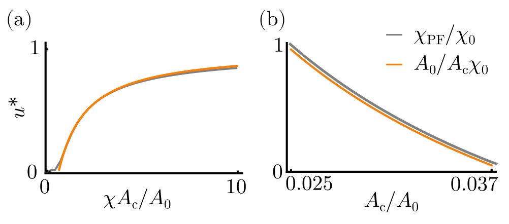
Figure 9: (a) Uniform fixpoints of Eq. (4) computed numerically (gray) and approximation from linearization of the response function $\sigma(s_{ij})$ around $s_{ij}=1$ [Eq. (79)], (orange), $h=4$. (b) Comparison between Eq. (80) (orange) and the steady-state contact area computed numerically along the supercritical pitchfork bifurcation line derived via continuation in MatCont (gray), $\gamma_{0}/2\gamma_{\rm{f}}=0.98$

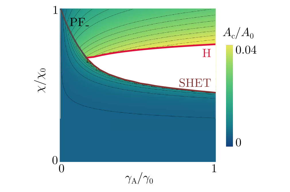
Figure 10: State diagram as shown in Fig. 2(a) for $\gamma_{0}/2\gamma_{\rm{f}}=0.98$. The color code indicates the normalized contact area at the fixpoint, i.e. at the uniform fixpoint state below the PF and SHET line and at the symmetry-broken fixpoints above the PF and Hopf line. The oscillatory regime between Hopf and SHET line is white as it does not contain any stable fixpoints.

.4 Shapes of asymmetric droplets

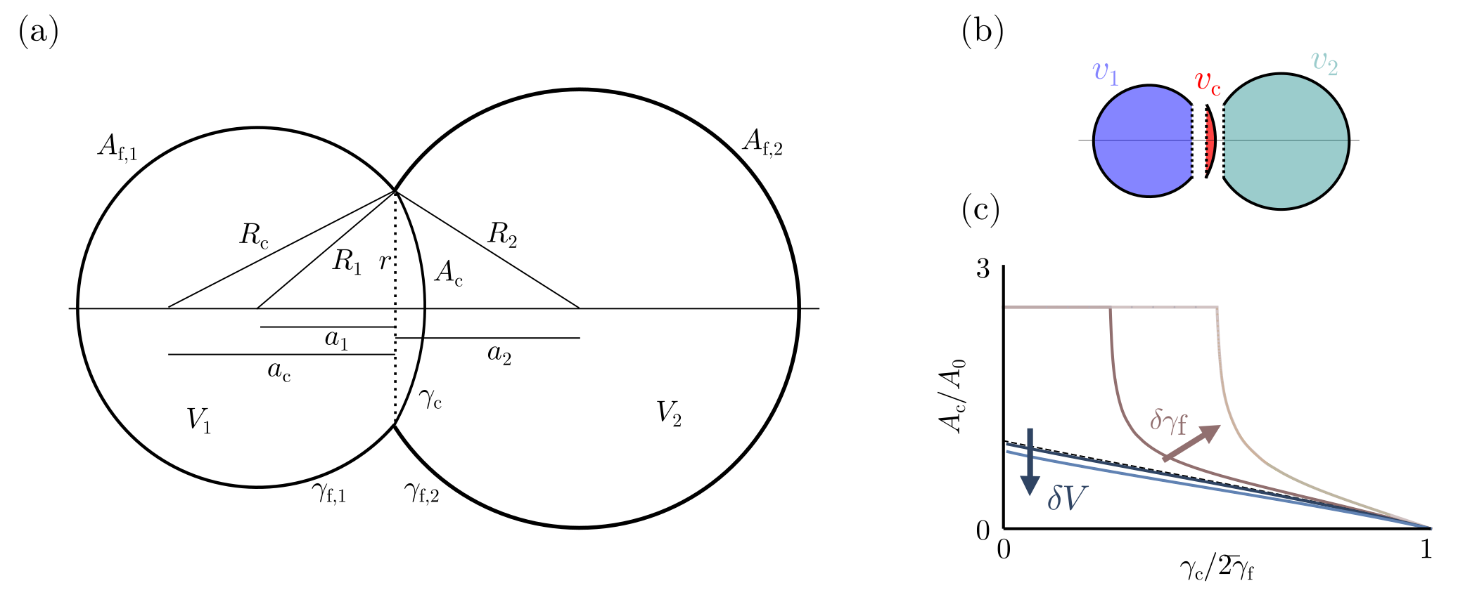
Figure 11: (a) Parameterization of a pair of asymmetric droplets adapted from [91]. (b) The droplet volumes can be expressed in terms of the three spherical cap volumes $v_{1},v_{2},v_{\rm{c}}$ (c) Differences in droplet volumes $\delta V/\bar{V}=\{0.25,0.5\}$ (blue) or outer interfacial tensions $\delta\gamma_{\rm{f}}/\bar{\gamma_{\rm{f}}}=\{0.25,0.5\}$ (brown) change how the contact area between the droplets depends on the tension ratio $\gamma_{\rm{c}}/2\bar{\gamma}_{\rm{f}}$

For pairs of droplets with unequal volumes ($V_{1}\neq V_{2}$) or outer surface tensions ($\gamma_{\rm{f},1}\neq\gamma_{\rm{f},2}$), Eq. (2) does not describe the size of the contact area. To derive the equilibrium shape and contact size of asymmetric droplets, we compute the minimum of the surface energy

$$E=\gamma_{\rm{c}}A_{\rm{c}}+\gamma_{\rm{f},1}A_{\rm{f},1}+\gamma_{\rm{f},2}A_{\rm{f},2}$$ (81)

under constant volume constraint. We follow the approach and use the parameterization introduced in [91], which is shown in Fig. 11(a). The droplet volumes can be expressed in terms of three spherical cap volumes $v_{i}$ with $i\in\{1,2,\rm{c}\}$ [Fig. 11(b)] such that

$$V_{1}=v_{1}+v_{c}$$ (82)

$$V_{2}=v_{2}-v_{c}.$$ (83)

Given the radii of curvature $R_{i}$ and the radius $r$ as shown in Fig. 11(a), we can define the length scales

$$a_{i}=\sqrt{R_{i}^{2}-r^{2}}$$ (84)

and surfaces

$$H_{i}(a_{i},r)=\frac{1}{2}\left(a_{i}^{2}+r^{2}+a_{i}\sqrt{a_{i}^{2}+r^{2}}\right),$$ (85)

which allows to express the spherical cap volumes as

$$v_{i}(a_{i},r)=\frac{\pi}{3}\left(a_{i}+\sqrt{a_{i}^{2}+r^{2}}\right)^{2}\left(2\sqrt{a_{i}^{2}+r^{2}}-a_{i}\right)$$ (86)

and the different droplet surfaces as

$$A_{i}(a_{i},r)=4\pi H_{i}(a_{i},r).$$ (87)

Using these definitions and expressing the outer surface tensions as $\gamma_{\rm{f},1}=\bar{\gamma}_{\rm{f}}+\delta\gamma_{\rm{f}},\gamma_{\rm{f},2}=\bar{\gamma}_{\rm{f}}-\delta\gamma_{\rm{f}}$, we can rewrite Eq. (81) as

$$\frac{E}{4\pi\bar{\gamma}_{\rm{f}}} =\left(1+\frac{\delta\gamma_{\rm{f}}}{\bar{\gamma}_{\rm{f}}}\right)H_{1}(a_{1},r)+\left(1-\frac{\delta\gamma_{\rm{f}}}{\bar{\gamma}_{\rm{f}}}\right)H_{2}(a_{2},r)$$

$$+2\left(\frac{\gamma_{\rm{c}}}{2\bar{\gamma}_{\rm{f}}}\right)H_{\rm{c}}(a_{\rm{c}},r)$$ (88)

with $\bar{\gamma}_{\rm{f}}=(\gamma_{\rm{f},1}+\gamma_{\rm{f},2})/2$. The minima in terms of the four parameters ($a_{1},a_{2},a_{\rm{c}},r$) under constant volume constraints $V_{1}=\bar{V}-\delta V,V_{2}=\bar{V}+\delta V$ were computed numerically, allowing to derive the size of the contact area $A_{\rm{c}}=4\pi H_{c}(a_{c},r)$ (Sec. 2).

.5 Literature values for reaction and diffusion rates

Khait et al. 2016 obtained quantitative estimates for many parameters governing the dynamics of Notch receptors and ligands (Tab. 1, [43]). The authors measured the 2D diffusion constant $D_{\mathrm{m}}$ and the endocytosis rate $k_{\rm{off}}$ in different cell lines and estimated the reaction rates from previously reported measurements of the binding kinetics for soluble molecules in 3D. The rate of receptor and ligand transport from the bulk to the surface $k_{\rm{on}}^{\rm{R}}c_{\rm{R}}^{0}$ and $k_{\rm{on}}^{\rm{L}}c_{\rm{L}}^{0}$ were estimated by assuming that the steady-state surface densities are $m_{\rm{R}}^{0}=$100\text{\,}{\mathrm{\SIUnitSymbolMicro m}}^{-2}$$ and $m_{\rm{L}}^{0}=$10\text{\,}{\mathrm{\SIUnitSymbolMicro m}}^{-2}$$ (i.e. there is an excess of receptors) when a cell is not in contact with another cell or ligand-coated substrate. In that case $m_{\rm{R}}=m_{\rm{R}}^{0}=k_{\rm{on}}^{\rm{R}}c_{\rm{R}}^{0}/k_{\rm{off}}^{\rm{R}}$ and $m_{\rm{L}}=m_{\rm{L}}^{0}=k_{\rm{on}}^{\rm{L}}c_{\rm{L}}^{0}/k_{\rm{off}}^{\rm{L}}$. $A_{\rm{c}}$ gives the range of contact areas for two spherical cells with radius $5\text{\,}\mathrm{\SIUnitSymbolMicro m}$ that keep a normalized contact area $A_{\rm{c}}/A_{0}\in[0,1]$ as assumed in this work.

Parameter	Symbol	Value
Endocytosis	$k_{\rm{off}}$	$0.02\text{\,}{\mathrm{s}}^{-1}$
Cleavage	$k_{\rm{s}}$	$0.34\text{\,}{\mathrm{s}}^{-1}$
Binding	$k_{+}$	$0.167\text{\,}{\mathrm{\SIUnitSymbolMicro m}}^{2}\text{\,}{\mathrm{s}}^{-1}$
Unbinding	$k_{-}$	$0.034\text{\,}{\mathrm{s}}^{-1}$
Diffusion coefficients	$D_{m_{\rm{R}}},D_{m_{\rm{L}}}$	$0.020.08\text{\,}{\mathrm{\SIUnitSymbolMicro m}}^{2}\text{\,}{\mathrm{s}}^{-1}$
Diffusion coefficient	$D_{m_{\mathrm{RL}}}$	$(D_{m_{\mathrm{R}}}+D_{m_{\mathrm{L}}})/4$
Exocytosis receptors	$k_{\rm{on}}^{\rm{R}}c_{\rm{R}}^{0}$	$2\text{\,}{\mathrm{\SIUnitSymbolMicro m}}^{-2}\text{\,}{\mathrm{s}}^{-1}$
Exocytosis ligands	$k_{\rm{on}}^{\rm{L}}c_{\rm{L}}^{0}$	$0.2\text{\,}{\mathrm{\SIUnitSymbolMicro m}}^{-2}\text{\,}{\mathrm{s}}^{-1}$
Contact area	$A_{\rm{c}}$	$0125\text{\,}{\mathrm{\SIUnitSymbolMicro m}}^{2}$

Table 1: Typical parameter values for reaction and diffusion rates of receptor and ligand molecules as reported in [43] and estimate of common cellular length scales

.6 Numerical methods

Physical quantity	Symbol	Values
Base line interfacial tension relative to outer surface tension	$\gamma_{0}/2\gamma_{\rm{f}}$	0.98
Base line interfacial tension relative to outer surface tension in a single adherent droplet	$(\gamma_{0}-\gamma_{\rm{m}})/2\gamma_{\rm{f}}$	0.98
Critical susceptibility without adaptive tension	$\chi_{0}$	40.604
Adaptive adhesion coefficient relative to outer surface tension	$\gamma_{\rm{A}}/2\gamma_{\rm{f}}$	Fig. 2(b): 0.294, Fig. 2(c): {0.15, 0.21, 0.23, 0.2352, 0.5} Fig. 2(d): 0.8 Fig. 2(e): {0.4, 0.6, 0.8} Fig. 3(c): 0.65
Relative signal susceptibility	$\chi/\chi_{0}$	Fig. 2(c): {0.1, 0.61, 0.604, 0.6021, 0.6, 0.95} Fig. 2(d): {0.4704, 0.7388} Fig. 3(c): {0.465, 0.5, 0.6, 0.74 }
Volume asymmetry	$\delta V/\bar{V}$	{0.25, 0.5}
Tension asymmetry	$\delta\gamma_{\rm{f}}/\bar{\gamma}_{\rm{f}}$	{0.25, 0.5}

Table 2: Parameter values.

Bifurcation analysis

The state and bifurcation diagrams presented in Fig. 2(a),(b), Fig. 3(a),(b) and Fig. 13 were computed via continuation with the MATLAB-based software package MatCont [92] (MatCont7p3 and MATLAB R2021a, scripts with details and numerical settings available at https://git.embl.de/dullwebe/dullweber2024. In general, initial fixpoints to initialize the continuation were computed by integration over time with random initial conditions using the Integrator Method ode45. The saddle-node homoclinic (HSN) and associated non-central homoclinic to saddle-node (NCH) bifurcations [Fig.3 3(b)] could only be obtained using the GUI-based version of MatCont7p3. For this, continuation of limit cycles was performed for $\gamma_{A}/\gamma_{0}=0.95$ and decreasing continuation parameter $\chi$ until the period reached a value close to 100 indicating the presence of a homoclinic causing period divergence. For different values of $\gamma_{A}/\gamma_{0}=0.95$, this point consistently coincides with the saddle-node bifurcation line. From the limit cycle of largest period, continuation of a HSN was initialized with InitStepsize 0.01, MinStepsize 0.05, MaxStepsize 0.1, MaxNewtonIters 3, MaxCorrIters 10, MaxTestIters 10, VarTolerance 1e-6, FunTolerance 1e-6, TestTolerance 1e-5, Adapt 1, MaxNumPoints 2000, CheckClosed 50 and Jacobian Increment 1e-05. Continuation of the HSN allows to detect the NCH codimension-2 point.

Results of the continuation were confirmed using simulations and analysis in Mathematica 13.0 (notebook available at https://git.embl.de/dullwebe/dullweber2024). Specifically, we tested the number and types of stable attractors in different parameter regimes with simulations using NDSolve and ParametricNDSolve with the equation simplification method Residuals. Fixpoints shown in the phase plots Fig. 3(c) were computed numerically in Mathematica from the intersections of nullclines. The oscillation amplitude [Fig. 2(d)] and period [Fig. 2(a)] were computed from the extrema of simulated trajectories, and checked against the dominant Fourier components.

Treatment of asymmetric droplet shapes

To obtain estimates of the equilibrium shapes of asymmetric droplets, we numerically computed the minimum of Eq. (88) in terms of the four parameters ($a_{1},a_{2},a_{\rm{c}},r$) and under the constant volume constraints $V_{1}=\bar{V}-\delta V,V_{2}=\bar{V}+\delta V$. We computed the contact area $A_{\rm{c}}=4\pi H_{c}$ for values of $\gamma_{\rm{c}}/2\bar{\gamma}_{\rm{f}}$ evenly spaced on the interval $[0,1]$. For unequal volumes ($V_{1}\neq V_{2}$), but identical outer surface tensions, we used a 5th order polynomial to fit a function $A_{\rm{c}}=A_{\rm{c}}(\gamma_{\rm{c}}/2\bar{\gamma}_{\rm{f}})$ on the interval $[0,1]$ using Mathematica’s function Fit with the default LevenbergMarquardt method [Fig. (11)(c)]. For droplets with asymmetric outer tension, but equal volumes, the droplet with higher outer tension is completely internalized if $\gamma_{\rm{c}}/2\bar{\gamma}_{\rm{f}}\leq\delta\gamma_{\rm{f}}$ [91], thus, we used a piecewise function to fit the contact area with $A_{\rm{c}}=2^{4/3}A_{0}$ on the interval $[0,\delta\gamma_{\rm{f}}]$. The interval $[\delta\gamma_{\rm{f}},1]$ was fitted with a combination of a rational function of the form $a+b/(\gamma_{\rm{c}}/2\gamma_{\rm{f}}-c)^{d}$ close to the threshold of internalisation with fit parameters $a-d$ and a 5th order polynomial [Fig. 11(c)]. Fits of the contact area were used for continuation in MatCont and simulations in Mathematica to derive the state diagrams shown in Fig. 3(a).

All codes are available at https://git.embl.de/dullwebe/dullweber2024.

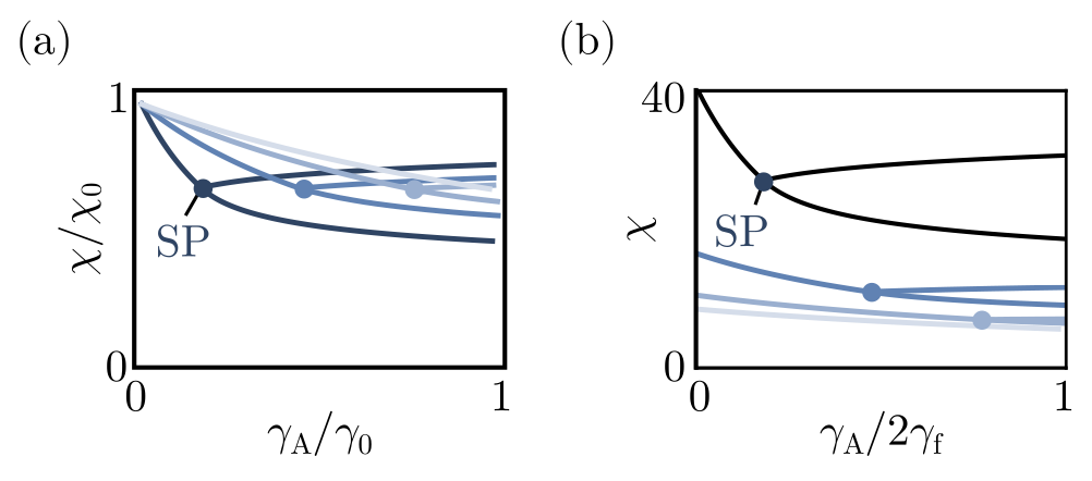
Figure 12: (a) State diagram as shown in Fig. 2(a) for different values of $\gamma_{0}/2\gamma_{\rm{f}}=\{0.98,0.95,0.92,0.9\}$ (dark to light blue) showing the saddle-node pitchfork (SP) codimension-2 bifurcation point and associated bifurcation lines. Note that $\chi_{0}$ is a function of $\gamma_{0}/2\gamma_{\rm{f}}$. (b) Same state diagram as in (a), but without normalization of $\chi$ and $\gamma_{\rm{A}}/2\gamma_{\rm{f}}$.

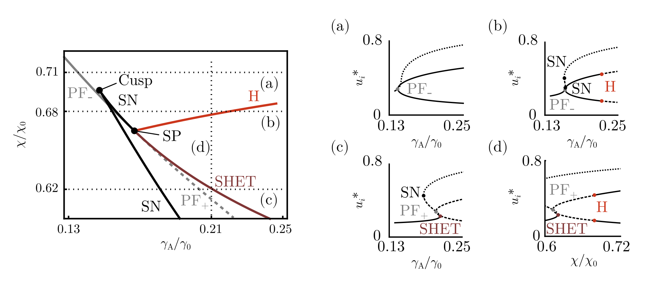
Figure 13: Bifurcation analysis close to the saddle-node pitchfork, Left: Enlarged view of the state diagram of the doublet in terms of normalized feedback control parameters shown in Fig. 2(a) close to the saddle-node pitchfork (SP) codimension-2 bifurcation point. (a) - (d) show stable (solid line) and unstable (dashed line) fixpoints and saddles (dotted line) computed for variation of one feedback parameter as indicated by dotted lines in the state diagram on the left. As the pitchfork interacts with one of the saddle-nodes (compare (b) and (c)), it changes from supercritical (PF_-) to subcritical (PF₊) and the saddle (SN) becomes a Saddle-Heteroclinic (SHET). In the parameter regime between the H and SHET bifurcation lines, the system has no stable fixpoints, but stable limit cycles. H: Hopf bifurcation. Diagrams were computed in MatCont, $\gamma_{0}/2\gamma_{\rm{f}}=0.98$.

References

- Mietke et al. [2019] A. Mietke, F. Jülicher, and I. F. Sbalzarini, Proceedings of the National Academy of Sciences 116, 29 (2019).
- Salbreux and Jülicher [2017] G. Salbreux and F. Jülicher, Physical Review E 96, 032404 (2017).
- Marchetti et al. [2013] M. C. Marchetti, J.-F. Joanny, S. Ramaswamy, T. B. Liverpool, J. Prost, M. Rao, and R. A. Simha, Reviews of modern physics 85, 1143 (2013).
- Shankar et al. [2022] S. Shankar, A. Souslov, M. J. Bowick, M. C. Marchetti, and V. Vitelli, Nature Reviews Physics 4, 380 (2022).
- Binysh et al. [2022] J. Binysh, T. R. Wilks, and A. Souslov, Science advances 8, eabk3079 (2022).
- Ray et al. [2023] S. Ray, J. Zhang, and Z. Dogic, Physical Review Letters 130, 238301 (2023).
- Araújo et al. [2023] N. A. Araújo, L. M. Janssen, T. Barois, G. Boffetta, I. Cohen, A. Corbetta, O. Dauchot, M. Dijkstra, W. M. Durham, A. Dussutour, et al., Soft matter 19, 1695 (2023).
- McEvoy and Correll [2015] M. A. McEvoy and N. Correll, Science 347, 1261689 (2015).
- Zhao et al. [2023] H. Zhao, A. Košmrlj, and S. S. Datta, arXiv preprint arXiv:2301.12345 (2023).
- Ziepke et al. [2022] A. Ziepke, I. Maryshev, I. S. Aranson, and E. Frey, Nature communications 13, 6727 (2022).
- Alberts et al. [2022a] B. Alberts, R. Heald, A. Johnson, D. Morgan, M. Raff, K. Roberts, and P. Walter, Molecular Biology of the Cell (WW Norton & Company, 2022) Chap. 15.
- Pisarchik and Hramov [2022] A. N. Pisarchik and A. E. Hramov, Multistability in Physical and Living Systems, Vol. 2 (Springer, 2022) Chap. 3.
- Sjöqvist and Andersson [2019] M. Sjöqvist and E. R. Andersson, Developmental biology 447, 58 (2019).
- Dullweber and Erzberger [2023] T. Dullweber and A. Erzberger, Current Opinion in Systems Biology , 100445 (2023).
- Sprinzak and Blacklow [2021] D. Sprinzak and S. C. Blacklow, Annual review of biophysics 50, 157 (2021).
- Erzberger et al. [2020] A. Erzberger, A. Jacobo, A. Dasgupta, and A. Hudspeth, Nature physics 16, 949 (2020).
- Luo et al. [2023] D. Luo, A. Maheshwari, A. Danielescu, J. Li, Y. Yang, Y. Tao, L. Sun, D. K. Patel, G. Wang, S. Yang, et al., Nature 614, 463 (2023).
- Shah et al. [2021] D. S. Shah, J. P. Powers, L. G. Tilton, S. Kriegman, J. Bongard, and R. Kramer-Bottiglio, Nature Machine Intelligence 3, 51 (2021).
- Venturini et al. [2020] V. Venturini, F. Pezzano, F. Catala Castro, H.-M. Häkkinen, S. Jiménez-Delgado, M. Colomer-Rosell, M. Marro, Q. Tolosa-Ramon, S. Paz-López, M. A. Valverde, et al., Science 370, eaba2644 (2020).
- Bodor et al. [2020] D. L. Bodor, W. Pönisch, R. G. Endres, and E. K. Paluch, Developmental cell 52, 550 (2020).
- Terryn et al. [2021] S. Terryn, J. Langenbach, E. Roels, J. Brancart, C. Bakkali-Hassani, Q.-A. Poutrel, A. Georgopoulou, T. G. Thuruthel, A. Safaei, P. Ferrentino, et al., Materials Today 47, 187 (2021).
- Ajeti et al. [2019] V. Ajeti, A. P. Tabatabai, A. J. Fleszar, M. F. Staddon, D. S. Seara, C. Suarez, M. S. Yousafzai, D. Bi, D. R. Kovar, S. Banerjee, et al., Nature physics 15, 696 (2019).
- Sun et al. [2023] G. Sun, R. Zhou, Z. Ma, Y. Li, R. Groß, Z. Chen, and S. Zhao, Nature Communications 14, 3476 (2023).
- Gov [2018] N. Gov, Philosophical Transactions of the Royal Society B: Biological Sciences 373, 20170115 (2018).
- Paluch and Heisenberg [2009] E. Paluch and C.-P. Heisenberg, Current Biology 19, R790 (2009).
- Linding and Klipp [2021] R. Linding and E. Klipp, Current Opinion in Systems Biology 27, 100354 (2021).
- Prasad and Alizadeh [2019] A. Prasad and E. Alizadeh, Trends in biotechnology 37, 347 (2019).
- Dullweber et al. [2023] T. Dullweber, R. Belousov, and A. Erzberger, Supplemental Material contains derivation of Eq.(2)-(5) from microscopic reaction-diffusion equations, a summary of the biological background and details of linear stability analysis, continuation and other numerical methods. (2023).
- Herszterg et al. [2023] S. Herszterg, M. de Gennes, S. Cicolini, A. Huang, C. Alexandre, M. Smith, H. Araujo, J.-P. Vincent, and G. Salbreux, bioRxiv , 2023 (2023).
- Corson et al. [2017] F. Corson, L. Couturier, H. Rouault, K. Mazouni, and F. Schweisguth, Science 356, eaai7407 (2017).
- Sitarska and Diz-Muñoz [2020] E. Sitarska and A. Diz-Muñoz, Current opinion in cell biology 66, 11 (2020).
- Chugh et al. [2017] P. Chugh, A. G. Clark, M. B. Smith, D. A. Cassani, K. Dierkes, A. Ragab, P. P. Roux, G. Charras, G. Salbreux, and E. K. Paluch, Nature cell biology 19, 689 (2017).
- Nambiar et al. [2009] R. Nambiar, R. E. McConnell, and M. J. Tyska, Proceedings of the National Academy of Sciences 106, 11972 (2009).
- Alberts et al. [2022b] B. Alberts, R. Heald, A. Johnson, D. Morgan, M. Raff, K. Roberts, and P. Walter, Molecular Biology of the Cell (WW Norton & Company, 2022) Chap. 19.
- Schwarz and Safran [2013] U. S. Schwarz and S. A. Safran, Reviews of Modern Physics 85, 1327 (2013).
- Maître et al. [2012] J.-L. Maître, H. Berthoumieux, S. F. G. Krens, G. Salbreux, F. Jülicher, E. Paluch, and C.-P. Heisenberg, science 338, 253 (2012).
- Bergert et al. [2015] M. Bergert, A. Erzberger, R. A. Desai, I. M. Aspalter, A. C. Oates, G. Charras, G. Salbreux, and E. K. Paluch, Nature cell biology 17, 524 (2015).
- Tjhung et al. [2012] E. Tjhung, D. Marenduzzo, and M. E. Cates, Proceedings of the National Academy of Sciences 109, 12381 (2012).
- Mayer et al. [2010] M. Mayer, M. Depken, J. S. Bois, F. Jülicher, and S. W. Grill, Nature 467, 617 (2010).
- Bormashenko [2017] E. Y. Bormashenko, Physics of wetting: phenomena and applications of fluids on surfaces (Walter de Gruyter GmbH & Co KG, 2017).
- Collier et al. [1996] J. R. Collier, N. A. Monk, P. K. Maini, and J. H. Lewis, Journal of Theoretical Biology 183, 429 (1996).
- Binshtok and Sprinzak [2018] U. Binshtok and D. Sprinzak, Molecular Mechanisms of Notch Signaling , 79 (2018).
- Khait et al. [2016] I. Khait, Y. Orsher, O. Golan, U. Binshtok, N. Gordon-Bar, L. Amir-Zilberstein, and D. Sprinzak, Cell reports 14, 225 (2016).
- Shaya et al. [2017] O. Shaya, U. Binshtok, M. Hersch, D. Rivkin, S. Weinreb, L. Amir-Zilberstein, B. Khamaisi, O. Oppenheim, R. A. Desai, R. J. Goodyear, et al., Developmental cell 40, 505 (2017).
- Blackbeard et al. [2012] N. Blackbeard, S. Osborne, S. O’Brien, and A. Amann, arXiv preprint arXiv:1210.4484 (2012).
- Nandagopal et al. [2018] N. Nandagopal, L. A. Santat, L. LeBon, D. Sprinzak, M. E. Bronner, and M. B. Elowitz, Cell 172, 869 (2018).
- Viswanathan et al. [2021] R. Viswanathan, J. Hartmann, C. Pallares Cartes, and S. De Renzis, The EMBO Journal 40, e107245 (2021).
- Sonnen and Janda [2021] K. F. Sonnen and C. Y. Janda, Biochemical Journal 478, 4045 (2021).
- Casani-Galdon and Garcia-Ojalvo [2022] P. Casani-Galdon and J. Garcia-Ojalvo, Current Opinion in Cell Biology 78, 102130 (2022).
- Purvis and Lahav [2013] J. E. Purvis and G. Lahav, Cell 152, 945 (2013).
- Pérez-Verdugo et al. [2023] F. Pérez-Verdugo, S. Banks, and S. Banerjee, arXiv preprint arXiv:2310.04950 (2023).
- Rombouts et al. [2023] J. Rombouts, J. Elliott, and A. Erzberger, EMBO reports , e57739 (2023).
- Di Talia and Vergassola [2022] S. Di Talia and M. Vergassola, Annual review of biophysics 51, 327 (2022).
- Corominas-Murtra and Petridou [2021] B. Corominas-Murtra and N. I. Petridou, Frontiers in Physics 9, 666916 (2021).
- Guirao and Bellaïche [2017] B. Guirao and Y. Bellaïche, Current opinion in cell biology 48, 113 (2017).
- Hausberg and Röger [2018a] S. Hausberg and M. Röger, Nonlinear Differential Equations and Applications NoDEA 25, 17 (2018a).
- Brauns et al. [2020] F. Brauns, J. Halatek, and E. Frey, Physical Review X 10, 041036 (2020).
- Ross et al. [2021] A. B. Ross, J. D. Langer, and M. Jovanovic, Molecular & Cellular Proteomics 20 (2021).
- Hausberg and Röger [2018b] S. Hausberg and M. Röger, Nonlinear Differential Equations and Applications NoDEA 25, 1 (2018b).
- Milo and Phillips [2015] R. Milo and R. Phillips, Cell biology by the numbers (Garland Science, 2015).
- Sankaran et al. [2009] J. Sankaran, M. Manna, L. Guo, R. Kraut, and T. Wohland, Biophysical journal 97, 2630 (2009).
- Shamir et al. [2016] M. Shamir, Y. Bar-On, R. Phillips, and R. Milo, Cell 164, 1302 (2016).
- Buccitelli and Selbach [2020] C. Buccitelli and M. Selbach, Nature Reviews Genetics 21, 630 (2020).
- Jacobson et al. [2019] K. Jacobson, P. Liu, and B. C. Lagerholm, Cell 177, 806 (2019).
- Trimble and Grinstein [2015] W. S. Trimble and S. Grinstein, Journal of Cell Biology 208, 259 (2015).
- Wyatt et al. [2016] T. Wyatt, B. Baum, and G. Charras, Current opinion in cell biology 38, 68 (2016).
- Tran-Son-Tay et al. [1991] R. Tran-Son-Tay, D. Needham, A. Yeung, and R. Hochmuth, Biophysical journal 60, 856 (1991).
- Maître and Heisenberg [2011] J.-L. Maître and C.-P. Heisenberg, Current opinion in cell biology 23, 508 (2011).
- Chu et al. [2004] Y.-S. Chu, W. A. Thomas, O. Eder, F. Pincet, E. Perez, J. P. Thiery, and S. Dufour, The Journal of cell biology 167, 1183 (2004).
- Ridgway et al. [2023] W. J. M. Ridgway, M. P. Dalwadi, P. Pearce, and S. J. Chapman, Phys. Rev. Lett. 131, 228302 (2023).
- van der Kolk et al. [2023] J. van der Kolk, F. Raßhofer, R. Swiderski, A. Haldar, A. Basu, and E. Frey, Phys. Rev. Lett. 131, 088201 (2023).
- Wadhams and Armitage [2004] G. H. Wadhams and J. P. Armitage, Nature reviews Molecular cell biology 5, 1024 (2004).
- Antunes and de Souza [2016] G. Antunes and F. M. S. de Souza, Methods in cell biology 132, 127 (2016).
- Murphy et al. [2022] K. Murphy, C. Weaver, L. Berg, G. Barton, and C. Janeway, Janeway’s Immunobiology, Vol. 10th ed. (W.W. Norton and Company, New York, NY, 2022, 2022).
- Alberts et al. [2022c] B. Alberts, R. Heald, A. Johnson, D. Morgan, M. Raff, K. Roberts, and P. Walter, Molecular Biology of the Cell (WW Norton & Company, 2022) Chap. 22.
- Guisoni et al. [2017] N. Guisoni, R. Martinez-Corral, J. Garcia-Ojalvo, and J. de Navascués, Development 144, 1177 (2017).
- Rusilowicz-Jones et al. [2022] E. V. Rusilowicz-Jones, S. Urbé, and M. J. Clague, Molecular Cell (2022).
- Beckstead et al. [2009] B. L. Beckstead, J. C. Tung, K. J. Liang, Z. Tavakkol, M. L. Usui, J. E. Olerud, and C. M. Giachelli, Journal of Biomedical Materials Research Part A: An Official Journal of The Society for Biomaterials, The Japanese Society for Biomaterials, and The Australian Society for Biomaterials and the Korean Society for Biomaterials 91, 436 (2009).
- Santillán [2008] M. Santillán, Mathematical Modelling of Natural Phenomena 3, 85 (2008).
- Olsauskas-Kuprys et al. [2013] R. Olsauskas-Kuprys, A. Zlobin, and C. Osipo, OncoTargets and therapy , 943 (2013).
- Ilagan et al. [2011] M. X. G. Ilagan, S. Lim, M. Fulbright, D. Piwnica-Worms, and R. Kopan, Science signaling 4, rs7 (2011).
- Fryer et al. [2004] C. J. Fryer, J. B. White, and K. A. Jones, Molecular cell 16, 509 (2004).
- Tveriakhina et al. [2023] L. Tveriakhina, G. Scanavachi, E. D. Egan, R. B. D. C. Correia, A. P. Martin, J. M. Rogers, J. S. Yodh, J. C. Aster, T. Kirchhausen, and S. C. Blacklow, bioRxiv 10.1101/2023.09.27.559780 (2023).
- Cohen et al. [2023] R. Cohen, S. Taiber, O. Loza, S. Kasirer, S. Woland, and D. Sprinzak, Science Advances 9, eadd2157 (2023).
- Cohen et al. [2022] R. Cohen, S. Taiber, O. Loza, S. Kasirer, S. Woland, and D. Sprinzak, Mechano-signaling feedback underlies precise inner hair cell patterning in the organ of corti, bioRxiv (2022), doi: 10.1101/2019.12.11.123456.
- Fischer-Friedrich et al. [2014] E. Fischer-Friedrich, A. A. Hyman, F. Jülicher, D. J. Müller, and J. Helenius, Scientific reports 4, 6213 (2014).
- Seib and Klein [2021] E. Seib and T. Klein, Biology of the Cell 113, 401 (2021).
- Vázquez-Ulloa et al. [2022] E. Vázquez-Ulloa, K.-L. Lin, M. Lizano, and C. Sahlgren, Critical Reviews in Biochemistry and Molecular Biology 57, 377 (2022).
- Kandachar and Roegiers [2012] V. Kandachar and F. Roegiers, Current opinion in cell biology 24, 534 (2012).
- Bray [2016] S. J. Bray, Nature reviews Molecular cell biology 17, 722 (2016).
- Maître et al. [2016] J.-L. Maître, H. Turlier, R. Illukkumbura, B. Eismann, R. Niwayama, F. Nédélec, and T. Hiiragi, Nature 536, 344 (2016).
- Dhooge et al. [2008] A. Dhooge, W. Govaerts, Y. A. Kuznetsov, H. G. E. Meijer, and B. Sautois, Mathematical and Computer Modelling of Dynamical Systems 14, 147 (2008).