SAGMAN: Stability Analysis of Graph Neural Networks on the Manifolds

Abstract

Modern graph neural networks (GNNs) can be sensitive to changes in the input graph structure and node features, potentially resulting in unpredictable behavior and degraded performance. In this work, we introduce a spectral framework known as SAGMAN for examining the stability of GNNs. This framework assesses the distance distortions that arise from the nonlinear mappings of GNNs between the input and output manifolds: when two nearby nodes on the input manifold are mapped (through a GNN model) to two distant ones on the output manifold, it implies a large distance distortion and thus a poor GNN stability. We propose a distance-preserving graph dimension reduction (GDR) approach that utilizes spectral graph embedding and probabilistic graphical models (PGMs) to create low-dimensional input/output graph-based manifolds for meaningful stability analysis. Our empirical evaluations show that SAGMAN effectively assesses the stability of each node when subjected to various edge or feature perturbations, offering a scalable approach for evaluating the stability of GNNs, extending to applications within recommendation systems. Furthermore, we illustrate its utility in downstream tasks, notably in enhancing GNN stability and facilitating adversarial targeted attacks.

1 Introduction

The advent of Graph Neural Networks (GNNs) has sparked a significant shift in machine learning (ML), particularly in the realm of graph-structured data (Keisler, 2022; Hu et al., 2020; Kipf & Welling, 2016; Veličković et al., 2017; Zhou et al., 2020). By seamlessly integrating graph structure and node features, GNNs yield low-dimensional embedding vectors that maximally preserve the graph structural information (Grover & Leskovec, 2016). Such networks have been successfully deployed in a broad spectrum of real-world applications, including but not limited to recommendation systems (Fan et al., 2019), traffic flow prediction (Yu et al., 2017), chip placement (Mirhoseini et al., 2021), and social network analysis (Ying et al., 2018). However, the enduring challenge in the deployment of GNNs pertains to their stability, especially when subjected to perturbations in the graph structure (Sun et al., 2020; Jin et al., 2020; Xu et al., 2019). Recent studies suggest that even minor alterations to the graph structure (encompassing the addition, removal, or rearrangement of edges) can have a pronounced impact on the performance of GNNs (Zügner et al., 2018; Xu et al., 2019). This phenomenon is particularly prominent in tasks such as node classification (Yao et al., 2019; Veličković et al., 2017; Bojchevski & Günnemann, 2019). The concept of stability here transcends mere resistance to adversarial attacks, encompassing the network’s ability to maintain consistent performance despite inevitable variations in the input data (graph structure and node features).

In the literature, a few studies are attempting to analyze GNN stability. Specifically, Keriven et al. first studied the stability of graph convolutional networks (GCN) on random graphs under small deformation. Later, Gama et al. and Kenlay et al. explored the robustness of various graph filters, which are then used to measure the stabilities of the corresponding (spectral-based) GNNs. However, these prior methods are limited to either synthetic graphs or specific GNN models.

In this work, we present SAGMAN, a novel framework devised to quantify the stability of GNNs through individual nodes. This is accomplished by assessing the resistance-distance distortions incurred by the map (GNN model) between low-dimensional input and output graph-based manifolds. To this end, we introduce a spectral approach for graph dimensionality reduction (GDR) to construct input/output graph-based manifolds that can well preserve effective-resistance distances between nodes. This approach allows transforming input graph data, including graph topology and node features that may originally lie in a high-dimensional space, into a low-dimensional input graph-based manifold. SAGMAN has nearly-linear algorithmic complexity and its data-centric nature allows SAGMAN to operate across various GNN variants, independent of label information, network architecture, and learned parameters, demonstrating its wide applicability. It is crucial to note that this study aims to offer significant insights for understanding and enhancing the stability of GNNs. The key technical contributions of this work are outlined below:

$\bullet$ To our knowledge, we are the first to propose a spectral method for evaluating node-level stability in GNNs. Our approach is distinguished by introducing input/output graph-based manifolds that can well preserve effective-resistance distances between nodes.

$\bullet$ We introduce a nonlinear GDR method and exploit PGMs to transform the original input graph into a low-dimensional graph-based manifold that can effectively preserve the original graph’s structural and spectral properties, enabling effective estimation of GNN stability.

$\bullet$ SAGMAN has been empirically evaluated and shown to be effective in assessing the stability of individual nodes across various GNN models in realistic graph datasets. Additionally, SAGMAN enables more potent adversarial target attacks and significantly enhances the stability of the GNNs.

$\bullet$ SAGMAN has a near-linear time complexity and is compatible with a wide range of GNN models and node label information. This makes SAGMAN highly adaptable for processing graphs of different sizes, various types of GNNs, and node-level tasks.

2 Background

2.1 Spectral Graph Theory

Spectral graph theory is a branch of mathematics that studies the properties of graphs through the eigenvalues and eigenvectors of matrices associated with the graph (Chung, 1997). Let $G=(V,E,w)$ denote an undirected graph $G$, $V$ denote a set of nodes (vertices), $E$ denote a set of edges and $w$ denote the corresponding edge weights. The adjacency matrix can be defined as:

$${A}(i,j)=\begin{cases}w(i,j)&\text{ if }(i,j)\in E\\ 0&\text{otherwise }\end{cases}\vspace{-5pt}$$ (1)

The Laplacian matrix of $G$ can be constructed by ${L={D}-{A}}$, where $D$ denotes the degree matrix.

Lemma 2.1.

(Courant-Fischer Minimax Theorem) The $k$-th largest eigenvalue of the Laplacian matrix $L\in\mathbb{R}^{|V|\times|V|}$ can be computed as follows:

$$\lambda_{k}(L)=\min_{dim(U)=k}\,{\max_{\begin{subarray}{c}u_{k}\in U\\ u_{k}\neq 0\end{subarray}}{\frac{u_{k}^{\top}Lu_{k}}{u_{k}^{\top}u_{k}}}}$$ (2)

Lemma 2.1 is the Courant-Fischer Minimax Theorem (Golub & Van Loan, 2013) for solving the eigenvalue problem: $Lu_{k}=\lambda_{k}u_{k}$. The generalized Courant-Fischer Minimax Theorem for solving generalized eigenvalue problem $L_{X}v_{k}=\lambda_{k}L_{Y}v_{k}$ can be expressed as follows:

Lemma 2.2.

(The Generalized Courant-Fischer Minimax Theorem) Given two Laplacian matrices $L_{X},L_{Y}\in\mathbb{R}^{|V|\times|V|}$ such that $null(L_{Y})\subseteq null(L_{X})$, the $k$-th largest eigenvalue of $L_{Y}^{+}L_{X}$ can be computed under the condition of $1\leq k\leq rank(L_{Y})$ by:

$$\lambda_{k}(L_{Y}^{+}L_{X})=\min_{\begin{subarray}{c}dim(U)=k\\ U\bot null(L_{Y})\end{subarray}}\,{\max_{v_{k}\in U}{\frac{v_{k}^{\top}L_{X}v_{k}}{v_{k}^{\top}L_{Y}v_{k}}}}.$$ (3)

2.2 Stability Analysis of ML Models on the Manifolds

The stability of an ML model refers to the ability of the model to produce consistent output despite small variations or noise in the input (Szegedy et al., 2013). Let $M$ denote an ML model, which operates on input $X$ to yield output $Y$, i.e., $Y=M(X)$. The stability of the ML model can be assessed by evaluating the distance distortions incurred by the maps between low-dimensional input and output manifolds. Specifically, a distance mapping distortion (DMD) metric has been introduced to evaluate the distance distortions between graph-based manifolds (Cheng et al., 2021). For two input data samples $p$ and $q$, the DMD metric denoted by $\delta^{M}(p,q)$ is defined as the ratio of the distance $d_{Y}(p,q)$ measured on the output graph-based manifold $G_{Y}=(V,E_{Y})$ to the one $d_{X}(p,q)$ on the input manifold $G_{X}=(V,E_{X})$ (Cheng et al., 2021):

$$DMD=\delta^{M}(p,q)\overset{\mathrm{def}}{=}\frac{d_{Y}(p,q)}{d_{X}(p,q)}.$$ (4)

By evaluating DMD for each pair of data samples, it becomes possible to assess the stability of the ML model: when two nearby data samples on the input manifold are mapped to two distant ones on the output manifold, it will imply a large local Lipschitz constant and thus poor stability of the ML model near these data samples.

2.3 Stability of GNNs

The stability of a GNN refers to its performance (output) stability in the presence of edge/node perturbations (Sun et al., 2020). This includes the ability to maintain the fidelity of predictions and outcomes when subjected to changes such as edge alterations or feature attacks. To elucidate, consider the scenario where the input graph data is subject to minor modifications, such as the addition or removal of a node, a change in node features, or a slight alteration in the graph structure. A desired GNN model is expected to exhibit good stability, wherein every predicted output or the graph embeddings do not change drastically in response to the aforementioned minor perturbations (Jin et al., 2020; Zhu et al., 2019). On the contrary, an unstable GNN would exhibit a considerable change in part of outputs or embeddings, potentially leading to erroneous inferences or predictions.

The importance of analyzing the stability of GNNs has been underlined by several recent studies. For instance, the vulnerability of GNNs to adversarial attacks has been studied in which small perturbations on targeted nodes can result in significant misclassifications (Zügner et al., 2018). In addition, although recent studies have investigated the stability issues of GNNs on synthetic graphs or specific models, they failed to develop a unified framework for evaluating the stability of GNNs.  (Keriven et al., 2020; Gama et al., 2020; Kenlay et al., 2021).

3 SAGMAN for Stability Analysis of GNNs

3.1 GNN Stability Analysis with DMDs is Nontrivial

When adopting the DMD metric for the stability analysis of GNN models, a natural question that arises is whether we can directly use the input graph structure of a GNN model as the input graph-based manifold for DMD calculations. Unfortunately, as shown in our empirical results reported in Table 2 and Appendix C, directly using the input graph topology for DMD evaluations does not lead to satisfactory stability analysis results. This is due to the fact that the original input graph data may not always lie near a low-dimensional space (Bruna et al., 2013), while meaningful DMD-based stability analysis requires that both input and output data samples lie near low-dimensional manifolds.

3.2 Overview of SAGMAN

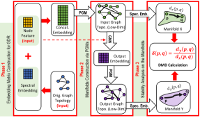
Figure 1: The proposed three-phase SAGMAN framework for stability analysis of GNNs on the manifolds.

To extend the applicability of the DMD metric to the GNN settings, we introduce a spectral framework, SAGMAN, for stability analysis of GNNs. A key ingredient of SAGMAN is a novel distance-preserving GDR algorithm for converting the original input graph data (including node features and graph topology) that may lie in high-dimensional space into a low-dimensional graph-based manifold. As shown in Figure 1, the proposed SAGMAN framework consists of three main phases: Phase 1 for creating the input graph embedding matrix (based on both node features and spectral graph properties) indispensable to the subsequent GDR step, Phase 2 for constructing low-dimensional input and output graph-based manifolds exploiting a probabilistic graphical model (PGM) approach, and Phase 3 for DMD-based node stability evaluation leveraging a spectral graph embedding scheme using generalized Laplacian eigenvalues/eigenvectors. A detailed exposition of our framework is presented in the following sections.

3.3 Phase 1: Embedding Matrix Construction for GDR

GDR via Laplacian Eigenmaps.

In this work, we exploit spectral graph embedding and the widely recognized nonlinear dimensionality reduction algorithm, Laplacian Eigenmaps (Belkin & Niyogi, 2003), for reducing the dimensionality of an input graph. The algorithm flow of Laplacian Eigenmaps starts with constructing an undirected (nearest-neighbor) graph where each node represents a (high-dimensional) data sample (vector) and each edge encodes the similarity between two data samples. Then the eigenvectors corresponding to the smallest eigenvalues of the graph Laplacian matrix are exploited for mapping each node (sample) into a low-dimensional space for preserving the local relationships between data samples.

Spectral Embedding with Eigengaps.

To apply Laplacian Eigenmaps for dimensionality reduction of a given graph with $N$ nodes, a straightforward approach is to first compute a $N\times N$ spectral embedding matrix using the complete set of graph Laplacian eigenvectors/eigenvalues (Ng et al., 2001), such that each node can be represented by an $N$-dimensional vector; next Laplacian Eigenmap will take this embedding matrix as input for the subsequent steps. However, computing the full set of eigenvalues/eigenvectors will be too expensive for large graphs. To address this complexity issue, a recent theoretical result on spectral graph clustering  (Peng et al., 2015) will be exploited in SAGMAN, which shows that the existence of a significant gap between two consecutive eigenvalues $\Upsilon(k)=\frac{\lambda_{k+1}}{\rho(k)}$, where $\rho(k)$ denotes the $k$-way expansion constant and $\lambda_{k+1}$ denotes the $(k+1)$-th smallest eigenvalue of the normalized Laplacian matrix, implies the existence of a $k$-way partition for which every cluster has low conductance, and that the underlying graph is a well-clustered graph.

Definition 3.1.

For a connected graph $G=(V,E,w)$ with its $k$ smallest nonzero Laplacian eigenvalues denoted by $0<\lambda_{1}\leq\lambda_{2}\leq\ldots\leq\lambda_{k}$ and their corresponding eigenvectors denoted by $u_{1},u_{2},\dots,u_{k}$, its weighted spectral embedding matrix is defined as $U_{k}=\left[\frac{u_{1}}{\sqrt{\lambda_{1}}},\dots,\frac{u_{k}}{\sqrt{\lambda_{k}}}\right]\in{\mathbb{R}^{|V|\times k}}$.

For a graph with a significant eigengap $\Upsilon(k)$, the above embedding matrix allows representing each node with a $k$-dimensional vector such that the effective-resistance distance between arbitrary node pairs can be well approximated by $d^{eff}({p,q})\approx|U_{k}^{\top}e_{p,q}|^{2}_{2}$, where ${e_{p}}\in\mathbb{R}^{|V|}$ denotes the standard basis vector with all zero entries except for the $p$-th entry being $1$, and ${e_{p,q}}=e_{p}-e_{q}$.

Eigengap for Graph Dimension Estimation.

Graph dimension is defined as the minimum integer that permits a ‘classical representation’ of the graph within an Euclidean space ($\mathbb{R}^{n}$) while preserving the unit length of all edges (Erdös et al., 1965). However, the precise quantification of either the graph dimension or the Euclidean dimension is computationally challenging, being an NP-hard problem (Schaefer, 2012). Fortunately, the existence of a significant eigengap $\Upsilon(k)$ implies the original graph can be very well represented in a $k$-dimensional space (Peng et al., 2015), and thus the graph dimensionality is approximately $k$. While precisely quantifying $\Upsilon(k)$ still remains challenging in practice, SAGMAN circumvents the need for the exact computation of graph dimensions. Instead, the identified eigengap acts as an indicative marker for assessing the suitability of SAGMAN for a specific graph: the ones with significant eigengaps will be more suitable for the SAGMAN framework since they can be well represented in low-dimensional space. Empirically, for datasets with the class number $c$, the value of $k$ can be approximated as $k\approx 10c$ to capture significant eigengaps effectively (Deng et al., 2022).

3.4 Phase 2: Manifold Construction via PGMs

While the original algorithm in Laplacian Eigenmaps suggests creating graph-based manifolds using $\epsilon$- or $k$-nearest-neighbor graphs, it is unclear whether the resulting graph-based manifolds can well preserve the effective-resistance distances on the original graph.

PGM for Graph Topology Learning from Data.

PGMs, also known as Markov Random Fields (MRFs), are powerful tools in machine learning and statistical physics for representing complex systems with intricate dependency structures (Roy et al., 2009). PGMs encode the conditional dependencies between random variables through an undirected graph structure. Recent results show that the graph structure learned through PGM will have its resistance distances encoding the Euclidean distances between their corresponding data samples  (Feng, 2021). Since each column vector in the embedding matrix $U_{k}$ in Definition 3.1 corresponds to a data sample for graph topology learning, the low-dimensional manifold constructed via PGM will well preserve the resistance distances in the original graph. However, the state-of-the-art method may require numerous iterations to achieve convergence (Feng, 2021), which limits its applicability in learning large graphs.

PGM via Spectral Sparsification.

In the proposed SAGMAN framework, we exploit PGMs for creating low-dimensional input graph-based manifolds using the embedding matrix $U_{k}$ in Definition 3.1, and the output manifold using GNN’s post-softmax vectors as shown in Figure 1. In the following, we provide a detailed description for constructing the input manifold, while the output one can be created in a similar way. For a given input embedding matrix $X=U_{k}\in{\mathbb{R}^{|V|\times k}}$, the maximum likelihood estimation (MLE) of the precision matrix $\Theta$ (PGM) can be obtained by solving the following convex problem (Dong et al., 2019):

$${\max_{\Theta}}:F(\Theta)=\log\det(\Theta)-\frac{1}{k}Tr({X^{\top}\Theta X})$$ (5)

where $\Theta={L}+\frac{1}{\sigma^{2}}I$, $Tr(\bullet)$ denotes the matrix trace, ${L}$ denotes the set of valid Laplacian matrices, $I$ denotes the identity matrix, and $\sigma^{2}>0$ denotes prior feature variance. Expanding the Laplacian matrix of $G=(V,E,w)$ with $L=\sum\limits_{\left({p,q}\right)\in E}{w_{p,q}}e_{p,q}e^{\top}_{p,q}$, where $w_{p,q}=\frac{1}{\|X^{\top}e_{p,q}\|_{2}^{2}}$ denotes the weight of the edge $(p,q)$, allows for expressing the objective function in Equation 5 as $F=F_{1}-\frac{1}{k}F_{2}$, where:

$$\begin{split}F_{1}&=\log\det(\Theta)=\sum\limits_{i=1}^{|V|}\log(\lambda_{i}+\frac{1}{\sigma^{2}})\\ F_{2}&=Tr({X^{\top}\Theta X})=\frac{Tr(X^{\top}X)}{\sigma^{2}}+\sum\limits_{\left({p,q}\right)\in E}{w_{p,q}}\|X^{\top}e_{p,q}\|_{2}^{2}.\end{split}$$ (6)

Taking partial derivatives with respect to $w_{p,q}$ leads to (Zhang et al., 2022):

$$\begin{split}\frac{\partial F_{1}}{\partial w_{p,q}}&=\sum\limits_{i=1}^{|V|}\frac{1}{\lambda_{i}+1/\sigma^{2}}\frac{\partial\lambda_{i}}{\partial w_{p,q}}=d^{eff}({p,q})\\ \frac{\partial F_{2}}{\partial w_{p,q}}&=\|X^{\top}e_{p,q}\|_{2}^{2}=d^{dat}({p,q})=\frac{1}{w_{p,q}},\end{split}$$ (7)

where $d^{eff}({p,q})$ and $d^{dat}({p,q})$ denote the effective-resistance distance and $\ell_{2}$ distance between nodes $p$ and $q$, respectively. To maximize the objective function $F$, an effective approach is to aggressively prune an initial graph (e.g. a nearest-neighbor graph) according to the gradients in Equation 7 by removing the edges with small resistance distance $d^{eff}({p,q})$ but large $\ell_{2}$ distance $d^{dat}({p,q})$ between nodes $p$ and $q$. This pruning strategy is equivalent to pruning edges with small distance ratios, defined as:

$$\rho_{p,q}=\frac{d^{eff}({p,q})}{d^{dat}({p,q})}=w_{p,q}d^{eff}({p,q}).$$ (8)

Since $\rho_{p,q}$ is exactly the edge sampling probability for spectral graph sparsification (Spielman & Teng, 2011), the proposed edge pruning strategy is equivalent to pruning the initial graph through spectral sparsification.

Spectral Sparsification via Graph Decomposition

To compute the edge sampling probability $\rho_{p,q}$ for each edge ($p,q$) requires solving Laplacian matrices multiple times (Spielman & Srivastava, 2008), which makes the original sparsification method computationally costly for large problems. An alternative approach for spectral sparsification employs a short-cycle graph decomposition scheme (Lemma 3.2) (Chu et al., 2020), which partitions an unweighted graph $G$ into multiple disjoint cycles by removing a fixed number of edges while ensuring a bound on the length of each cycle. In the last, the algorithm combines short-cycle decomposition with low-stretch spanning trees (LSSTs) to construct the sparsified graph for preserving the spectral properties of the original graph (Liu et al., 2019). However, such methods can only handle unweighted graphs.

Lemma 3.2.

Spectral sparsification of an undirected graph $G$ with its Laplacian denoted by $L_{G}$ can be obtained by leveraging a short-cycle decomposition algorithm, which returns a sparsified graph $H$ with its Laplacian denoted by $L_{H}$ such that for all real vectors $x$, $x^{\top}L_{G}x\approx x^{\top}L_{H}x$ (Chu et al., 2020).

As a substantial extension of prior short-cycle-based algorithms, we introduce an improved spectral sparsification algorithm, as shown in Figure 2. Our approach utilizes a low-resistance-diameter (LRD) decomposition scheme to limit the length of each cycle as measured by the effective-resistance metric. This method is particularly effective for sparsifying weighted graphs. The key idea in our method is to efficiently compute the effective resistance of each edge (see details in Appendix D) and leverage a multi-level framework to decompose the graph into several disjoint cycles bounded by an effective-resistance threshold. As shown in Figure 2, the subgraph corresponding to each node cluster will be sparsified into an LSST, while inter-cluster (bridge-like) edges will be retained to preserve the original structural properties. It is worth noting that these inter-cluster edges can be inserted into the original graph to significantly enhance the stability of GNN models, as shown in Table 4.

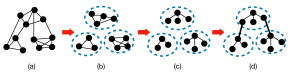
Figure 2: The proposed spectral sparsification algorithm. (a) The initial graph. (b) LRD decomposition for graph clustering. (c) LSSTs for pruning non-critical edges within clusters. (d) The final graph-based manifold with two inter-cluster edges.

3.5 Phase 3: Stability Analysis on the Manifolds

DMD with Resistance Distance Metric.

Let $M$ denote the mapping function of an ML model that operates on input $X$ to yield output $Y$, i.e., $Y=M(X)$. The effective-resistance distances between data samples $p$ and $q$ on the input and output graph-based manifolds can be computed by $d^{eff}_{X}(p,q)=e_{p,q}^{\top}L_{X}^{+}e_{p,q}$, and $d^{eff}_{Y}(p,q)=e_{p,q}^{\top}L_{Y}^{+}e_{p,q}$, respectively, where $L_{X}^{+}$ and $L_{Y}^{+}$ denote the Moore–Penrose pseudoinverses of graph Laplacian matrices of the input and output graph-based manifolds, respectively. For any arbitrary node pair $p$ and $q$ on graph-based manifolds, the maximum DMD measured using resistance-distance metric can be obtained by solving the following combinatorial optimization problem (Cheng et al., 2021):

$$\delta_{max}^{M}(p,q)=\mathop{\max_{\forall p,q\in V}}_{p\neq q}\frac{d^{eff}_{Y}(p,q)}{d^{eff}_{X}(p,q)}=\mathop{\max_{\forall p,q\in V}}_{p\neq q}\frac{e_{p,q}^{\top}L_{Y}^{+}e_{p,q}}{e_{p,q}^{\top}L_{X}^{+}e_{p,q}}.$$ (9)

Then the best Lipschitz constant $K^{*}$ of the mapping function $M$ is upper bounded by the largest eigenvalue of $L_{Y}^{+}L_{X}$ according to Lemma 2.2 (Cheng et al., 2021):

$$\lambda_{max}(L_{Y}^{+}L_{X})\geq K^{*}\geq{\delta_{max}^{M}(p,q)}.$$ (10)

Node Stability Score via Spectral Embedding.

Recent theoretical advancements (Cheng et al., 2021) motivate us to exploit the largest generalized eigenvalues and their corresponding eigenvectors for the stability assessment of individual nodes in GNNs. Specifically, we first compute the weighted eigensubspace matrix $V_{s}\in{\mathbb{R}^{|V|\times s}}$ for spectral embedding on the input graph-based manifold $G_{X}=(V,E_{X})$ with $V$ nodes: $V_{s}\overset{\mathrm{def}}{=}\left[{v_{1}}{\sqrt{\zeta_{1}}},...,{v_{s}}{\sqrt{\zeta_{s}}}\right],$ where $\zeta_{1},\zeta_{2},...,\zeta_{s}$ represent the first $s$ largest eigenvalues of $L_{Y}^{+}L_{X}$ and $v_{1},v_{2},...,v_{s}$ are the corresponding eigenvectors. Subsequently, $G_{X}$ is embedded using $V_{s}$, where each node is represented by an $s$-dimensional embedding vector. The stability of an edge $(p,q)\in E_{X}$ can be then estimated by computing the spectral embedding distance between two end nodes $p$ and $q$. The stability score of a node $p$ can be further computed as follows:

$$\begin{split}\textbf{score}(p)\overset{\mathrm{def}}{=}\frac{1}{|\mathbb{N}_{X}(p)|}\sum_{q_{i}\in\mathbb{N}_{X}(p)}\left(\|V_{s}^{\top}e_{p,q_{i}}\|_{2}^{2}\right)\\ \propto\frac{1}{|\mathbb{N}_{X}(p)|}\sum_{q_{i}\in\mathbb{N}_{X}(p)}\left(\delta^{M}(p,q_{i})\right)^{3}\end{split}$$ (11)

where $\mathbb{N}_{X}(p)$ represents the set of neighbors of node $p$ in the input graph-based manifold $G_{X}$. This node stability score can effectively serve as a surrogate for the local Lipschitz constant, which is analogous to $\|\nabla_{X}F(p)\|$ under the manifold setting (Cheng et al., 2021). For a more detailed exposition, please refer to Appendix F.

3.6 Complexity of SAGMAN

The detailed SAGMAN flow is shown in Appendix B. For spectral graph embedding, we can exploit fast multilevel eigensolvers that allow computing the first $c$ Laplacian eigenvectors in nearly-linear time $O(c|V|)$ without loss of accuracy (Zhao et al., 2021). The $k$-nearest neighbor algorithm (Malkov & Yashunin, 2018) has a nearly-linear computational complexity $O(|V|\log|V|)$. Spectral sparsification via LRD decomposition has $O(|V|dm)$ time complexity. By leveraging fast generalized eigensolvers (Koutis et al., 2010; Cucuringu et al., 2016) all DMD values can be computed within $O(|E|)$ time, where the $V$/$E$ denotes the number of nodes/edges, $d$ denotes the average degree of the matrix, and $m$ is the order of Krylov subspace. The SAGMAN is capable of handling very large datasets due to its nearly-linear time complexity. For instance, SAGMAN takes $391.15$ seconds to process the “ogbn-arxiv” dataset with $169,343$ nodes and $1,166,243$ edges on a system with an $i9$ $10900kf$ processor, $32GB$ RAM, and an NVIDIA Titan RTX $24GB$ GPU.

4 Experiments

In this paper, We conduct a comparison between exact resistance distances from the original graph and their approximations derived from the constructed manifold. Then, we present a series of fundamental numerical experiments designed to showcase the effectiveness of our proposed metric in quantifying the stability of GNNs under various perturbations in node features and edges. Additionally, we extend our analysis to the realm of recommendation systems, demonstrating how our metric measures their stability effectively. Furthermore, we highlight the efficacy and efficiency of our SAGMAN-guided approach in executing graph adversarial attacks. Then, we show how to significantly enhance the stability of GNN models leveraging the low-dimensional graph-based input manifold created by SAGMAN. Lastly, We present the runtime performance of SAGMAN across various graph scales.

Experimental Setup. See Appendix E for detailed descriptions of all graph datasets used in this work. We employ the most popular backbone GNN models including GCN (Kipf & Welling, 2016), GPRGNN (Chien et al., 2020), GAT (Veličković et al., 2017), APPNP (Gasteiger et al., 2018), and ChebNet (Defferrard et al., 2016). The recommendation system is based on PinSage (Ying et al., 2018). Perturbations include Gaussian noise evasion attacks and adversarial attacks (DICE (Waniek et al., 2018), Nettack (Zügner et al., 2018), and FGA (Chen et al., 2018)). The input graph-based manifolds are constructed using graph adjacency and node features, while the output graph-based manifold is created using post-softmax vectors. To showcase SAGMAN’s effectiveness in differentiating stable from unstable nodes, we apply SAGMAN to select $1\%$ of the entire dataset as stable nodes, and another $1\%$ as unstable nodes. This decision stems from that only a portion of the dataset significantly impacts model stability (Cheng et al., 2021; Hua et al., 2021; Chang et al., 2017). Additional evaluation results on the entire dataset can be found in Appendix G. We quantify output perturbations using cosine similarity and Kullback-Leibler divergence (KLD). Additional insights on cosine similarity, KLD, and accuracy can be found in Appendix A. For a large-scale dataset “ogbn-arxiv”, due to its higher output dimensionality, we focus exclusively on accuracy comparisons. This decision is informed by the KLD estimator’s $n^{-\frac{1}{d}}$ convergence rate (Roldán & Parrondo, 2012), where $n$ is the number of samples and $d$ is the dimension. In this paper, our spectral embedding method consistently utilizes the smallest $50$ eigenpairs for all experiments, unless explicitly stated otherwise.

4.1 Evaluation of Graph Dimension Reduction (GDR)

There is a valid concern about how much the constructed input graph-based manifold might change the original graph’s structure. To this end, we compare the exact resistance distances calculated using the complete set of eigenpairs with approximate ones estimated using the embedding matrix $U_{k}$ in Definition 3.1 where various $k$ values have been considered in Table 1. This empirical evidence shows that using a small number of eigenpairs can effectively approximate the original effective-resistance distances. Table 2 empirically shows the SAGMAN-guided stability analysis with GDR can always distinguish stable and unstable nodes, while the one without GDR can not. Additional related results for various datasets and GNNs have been reported in Appendix C.

Table 1: Resistance-distance preservation for the Cora graph, evaluating $100$ randomly selected node pairs. Larger correlation coefficients (CC) indicate more accurate estimations.

$k$	20	30	50	100	200	400	500
CC	0.69	0.78	0.82	0.87	0.93	0.97	0.99

Table 2: Nettack adversarial attack targeting SAGMAN-selected Cora samples in GCN. Better results are highlighted in bold.

Nettack Level	Cosine Similarities: Stable/Unstable
	w/o GDR	w/ GDR
1	0.90/0.96	0.99/0.90
2	0.84/0.93	0.98/0.84
3	0.81/0.91	0.97/0.81

Table 3: Comparison of Nettack/FGA error rates for 40 nodes selected using Nettack’s recommendation, confidence ranking, and SAGMAN. All nodes chosen by SAGMAN-guided methods are correctly classified before perturbation. Better results are highlighted in bold.

Dataset	Nettack’s Recommendation Nettack/FGA Error Rate	Confidence Ranking Nettack/FGA Error Rate	SAGMAN Nettack/FGA Error Rate
Cora	$0.725/0.850$	$0.925/0.775$	0.975/0.975
Cora-ml	$0.750/0.850$	$0.800/0.700$	0.950/0.950
Citeseer	$0.800/0.875$	$0.925/0.950$	1.000/0.975
Pubmed	$0.750/0.875$	$0.750/0.925$	0.825/0.950

Table 4: Error rates for the unstable dataset selected by SAGMAN. ‘Clean’ denotes the original graph without perturbations, while ‘Perturbed’ corresponds to the graph after a Nettack evasion attack. ‘Size’ indicates the fraction of the SAGMAN-selected nodes.

Cora	Original Graph	Enhanced Graph
Size	Clean/Perturbed	Clean/Perturbed
1%	0.000/0.791	0.000/0.000
5%	0.008/0.862	0.000/0.000
10%	0.008/0.903	0.008/0.008
15%	0.021/0.927	0.064/0.067
20%	0.024/0.921	0.078/0.086

4.2 Metrics for GNN Stability Evaluation

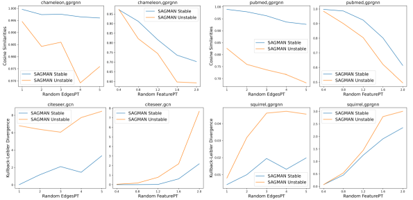
Figure 3: The horizontal axes, denoted by $X$, represent the magnitude of perturbation applied. ‘Random EdgesPT’ refers to the DICE adversarial attack scenario, in which pairs of nodes with different labels are connected and pairs with the same label are disconnected, with the number of pairs being equal to $X$. ‘Random FeaturePT’ indicates the application of Gaussian noise perturbation, expressed as $FM+X\eta$, where $FM$ denotes the feature matrix and $\eta$ represents Gaussian noise. The upper and lower subfigures illustrate the cosine similarity and the Kullback–Leibler Divergence (KLD). ‘SAGMAN Stable/Unstable’ denotes the samples that are classified as stable or unstable by SAGMAN, respectively.

We demonstrate the capability of SAGMAN for empirically distinguishing between stable samples and unstable samples in Figure 3. More results regarding different datasets, GNNs, and Nettack attacks are available in Appendix E. It illustrates our metric proves its effectiveness. Last, we report accuracy differences regarding large-scale datasets in Figure 4

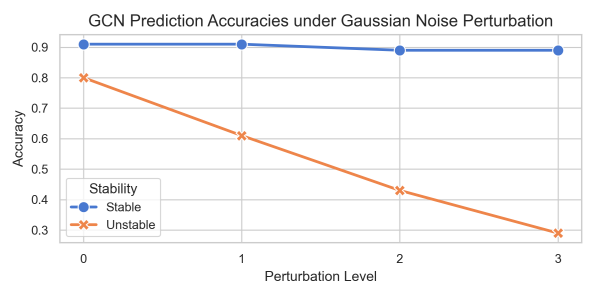
Figure 4: SAGMAN-selected stable/unstable samples for the ”ogbn-arxiv” dataset. We report the GCN prediction accuracies under different levels of Gaussian Noise Perturbation $FM+X\eta$, where $FM$ denotes the feature matrix, $\eta$ represents Gaussian noise, and $X$ is the noise perturbation level.

4.3 Stability of GNN-based Recommendation Systems

Our evaluation employs the PinSage GNN framework (Ying et al., 2018), utilizing the MovieLens 1M dataset (Harper & Konstan, 2015). To construct the input graph, we homogenize various node and edge types into a unified format, followed by calculating the weighted spectral embedding matrix $U_{k}$, which is defined in Definition 3.1. We then extract user-type samples from this matrix to build the low-dimensional input (user) graph-based manifold. To create the output graph-based manifold, we use PinSage’s final output including the top-$10$ recommended items for each user. An output (user) graph-based manifold is subsequently constructed based on Jaccard similarity measures. Table 5 clearly showcases the effectiveness of SAGMAN in differentiating between stable and unstable users.

Table 5: Comparison of the mean Jaccard similarity (MJS) between SAGMAN-selected stable and unstable users at a perturbation level ($l$) ranging from $1$ to $5$ where each selected user is connected to $l$ randomly chosen new items in the input graph. The MJS is computed over $20$ iterations for each perturbation level.

Per. Lev. ($l$)	Stable Users	Unstable Users
1	0.8513	0.7885
2	0.8837	0.7955
3	0.8295	0.8167
4	0.8480	0.8278
5	0.8473	0.7794

4.4 SAGMAN-guided Adversarial Targeted Attack

Our GNN training methodology is adapted from the approach delineated by (Jin et al., 2021). We adopt GCN as our base model for Citeseer, Cora, Cora-ml, and Pubmed, with Nettack and FGA serving as the benchmark attack methods. For comparison, target node selection follows Nettack’s recommendation (Zügner et al., 2018), SAGMAN-guided strategies, and a heuristic confidence ranking (Chang et al., 2017). Table 3 shows the error rates after Nettack and FGA attacks. As observed, the SAGMAN-guided attack outperforms both Nettack’s recommendation and confidence ranking, leading to more effective Nettack and FGA attacks. Furthermore, the SAGMAN-guided FGA attack (Chen et al., 2018) also demonstrates superior effectiveness.

4.5 SAGMAN-guided GNN Stability Enhancement

To improve the stability of a GNN model, a naive approach is to replace the entire input graph with the low-dimensional graph-based manifold for GNN predictions. However, due to the significantly increased densities in the graph-based manifold, the GNN prediction accuracy may also be influenced.

To achieve a flexible tradeoff between model stability and prediction accuracy, we only modify the top few most unstable nodes identified by SAGMAN. Specifically, for the most unstable nodes we only select the inter-cluster edges, as shown in Figure 2 (d), from the input graph-based manifold and insert them into the original graph. Since the inter-cluster (bridge-like) edges are mostly spectrally critical (with high sampling probabilities defined in Equation 8), adding them to the original graph will mostly significantly alter the structural (spectral) properties of the original graph.

Table 4 presents the error rates for both the original and the enhanced graphs. Nettack was employed to perturb SAGMAN-selected samples within each graph. Notably, reintegrating selected edges into the original graph significantly diminished the error rate when subjected to adversarial evasion attacks.

4.6 Runtime Scalability of SAGMAN

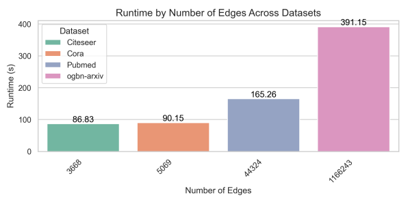
Figure 5: SAGMAN’s runtime across datasets

Figure 5 demonstrates the high efficiency of SAGMAN in handling large graph datasets, attributed to its near-linear time complexity.

5 Conclusions

In this work, we present SAGMAN, a novel framework for analyzing the stability of GNNs through individual nodes, which is achieved by assessing the resistance-distance distortions incurred by the maps between low-dimensional input and output graph-based manifolds. A key component in SAGMAN is a novel graph dimensionality reduction (GDR) approach for constructing resistance-preserving input/output graph-based manifolds. SAGMAN achieves promising performance in GNN stability analysis, leading to significantly enhanced targeted attacks and GNN stability. The current SAGMAN framework is most effective for handling graphs that can be well represented in low-dimensional space and have large eigengaps.

Appendix A Metrics for Assessing GNN Stability

In the context of single-label classification in graph nodes, consider an output vector $\mathbf{y}=[y_{1},y_{2},...,y_{k}]$ corresponding to an input $\mathbf{x}$, where $k$ represents the total number of classes. The model’s predicted class is denoted as $\hat{y}=\text{argmax}_{i}(y_{i})$. Now, let’s assume that the output vector transforms to $\mathbf{y^{\prime}}=[y^{\prime}_{1},y^{\prime}_{2},...,y^{\prime}_{k}]$, while preserving the ordinality of the elements, i.e., if $y_{i}>y_{j}$, then $y^{\prime}_{i}>y^{\prime}_{j}$. This condition ensures that $\hat{y^{\prime}}=\text{argmax}_{i}(y^{\prime}_{i})=\hat{y}$.

Relying solely on model accuracy can be deceptive, as it is contingent upon the preservation of the ordinality of the output vector elements, even when the vector itself undergoes significant transformations. This implies that the model’s accuracy remains ostensibly unaffected as long as the ranking of the elements within the output vector is conserved. However, this perspective neglects potential alterations in the model’s prediction confidence levels.

In contrast, the cosine similarity provides a more holistic measure as it quantifies the angle between two vectors, thereby indicating the extent of modification in the output direction. This method offers a more granular insight into the impact of adversarial attacks on the model’s predictions.

Moreover, it is crucial to consider the nature of the output space, $Y$. In situations where $Y$ forms a probability distribution, a common occurrence in classification problems, the application of a distribution distance measure such as the Kullback-Leibler (KL) divergence is typically more suitable. Unlike the oversimplified perspective of accuracy, these measures can provide a nuanced understanding of the degree of perturbation introduced in the predicted probability distribution by an adversarial attack. This additional granularity can expose subtle modifications in the model’s output that might be missed when solely relying on accuracy as a performance metric.

Appendix B Algorithm Flow of SAGMAN

The Algorithm 1 shows the key steps in SAGMAN. The process of obtaining low-dimensional graphs $G_{X}$ and $G_{Y}$ involves several steps, starting with the reduction of the graph dimension of $G_{X}$ using the weighted spectral embedding matrix. This matrix is denoted as $U_{k}$, which is defined in Definition 3.1. Following the approach suggested by (Deng et al., 2022), we enhance the graph construction by concatenating node features with dominant eigenvectors. The next step involves constructing the input PGM. This is achieved by first constructing a dense graph using the embedding matrix $E$, and then sparsifying this dense graph through short-cycle decomposition. The structure of the low-dimensional graph $G_{X}$ is obtained with the assistance of the input PGM. This graph, along with the node feature $X$, is then fed into a GNN to generate the output matrix $Y$. To construct the output PGM, we follow a similar process as with the input PGM: we construct a dense graph with $Y$ and sparsify the dense graph via short-cycle decomposition. This results in the low-dimensional graph $G_{Y}$, which is obtained with the aid of the output PGM. From the graphs $G_{X}$ and $G_{Y}$, we derive the Laplacian matrices $L_{X}$ and $L_{Y}$, respectively. The metric $\delta^{M}(p,q_{i})$ can then be calculated by evaluating $V_{N}^{\top}e_{p,q_{i}}$. In Appendix F, we provide a more detailed explanation of the relationship between $V_{N}^{\top}e_{p,q_{i}}$ and $\delta^{M}(p,q_{i})$. Finally, the node $p$ DMD score is obtained by averaging the DMD scores of node $p$ and its neighbors.

Algorithm 1 The algorithm flow of SAGMAN

  Input: Input graph $G$, Node features $X$, GNN

  Output: Stability (DMD) scores for all nodes

  $U_{N}\leftarrow\text{compute\_weighted\_spectral\_embedding}(G)$

  $V\leftarrow\text{concatenate}(X,U_{N})$

  $kNN\_dense\_graph\leftarrow\text{construct\_kNN\_graph}(E)$

  $input\_PGM\leftarrow\text{sparse\_graph}(kNN\_dense\_graph)$

  $G_{X}\leftarrow\text{get\_low\_dimensional\_graph}(input\_PGM)$

  $Y\leftarrow\text{GNN}(G_{X},X)$

  $kNN\_dense\_graph\_Y\leftarrow\text{construct\_kNN\_graph}(Y)$

  $output\_PGM\leftarrow\text{sparse\_graph}(kNN\_dense\_graph\_Y)$

  $G_{Y}\leftarrow\text{get\_low\_dimensional\_graph}(output\_PGM)$

  $L_{X}\leftarrow\text{compute\_laplacian}(G_{X})$

  $L_{Y}\leftarrow\text{compute\_laplacian}(G_{Y})$

  $V_{k}\leftarrow\text{calculate\_generalized\_eigenvectors}(L_{X},L_{Y})$

  for each node $p$ in $G_{X}$ do

     Compute the node stability score for $p$ in $G_{X}$:

$$score(p)=\frac{1}{|\mathbb{N}_{X}(p)|}\sum_{q_{i}\in\mathbb{N}_{X}(p)}\left(\|V_{k}^{\top}e_{p,q}\|^{2}_{2}\right)$$

  end for

Appendix C SAGMAN without GDR

In this study, we present the outcomes of stability quantification using original input and output graphs, as depicted in Figure 6. Our experimental findings underscore a key observation: SAGMAN without GDR does not allow for meaningful estimations of the GNN stability.

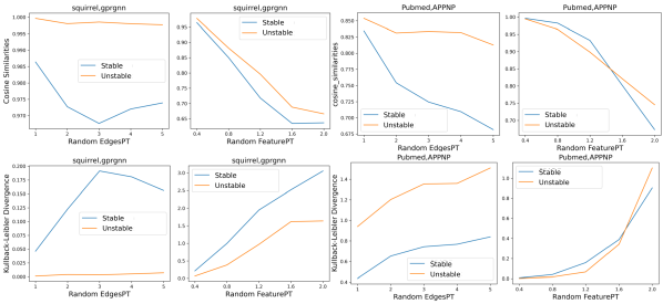
Figure 6: The horizontal axes, denoted by $X$, represent the magnitude of perturbation applied. ‘Random EdgesPT’ refers to the DICE adversarial attack scenario, in which pairs of nodes with different labels are connected and pairs with the same label are disconnected, with the number of pairs being equal to $X$. ‘Random FeaturePT’ indicates the application of Gaussian noise perturbation, expressed as $FM+X\eta$, where $FM$ denotes the feature matrix and $\eta$ represents Gaussian noise. The upper and lower subfigures illustrate the cosine similarity and the Kullback–Leibler Divergence (KLD). ‘Stable/Unstable’ denotes the samples that are classified as stable or unstable without GDR, respectively.

Appendix D Fast Effective-Resistance Estimation for LRD Graph Decomposition

The effective-resistance between nodes $(p,q)\in|V|$ can be computed using the following equation:

$$d^{eff}({p,q})=\sum\limits_{i=2}^{N}\frac{(u_{i}^{\top}e_{p,q})^{2}}{u_{i}^{\top}L_{G}u_{i}},$$ (12)

where $u_{i}$ represents the eigenvector corresponding to $\sigma_{i}$ eigenvalue of $L_{G}$ and $e_{p,q}=e_{p}-e_{q}$. To avoid the computational complexity associated with computing eigenvalues/eigenvectors, we leverage a scalable algorithm that approximates the eigenvectors by exploiting the Krylov subspace. In this context, given a nonsingular matrix $A_{N\times N}$ and a vector $c\neq 0\in\mathbb{R}^{N}$, the order-$(m)$ Krylov subspace generated by $A$ from $c$ is defined as:

$$\kappa_{m}(A,c):=span(c,Ac,A^{2}c,...,A^{m-1}c),$$ (13)

where $c$ denotes a random vector, and $A$ denotes the adjacency matrix of graph $G$. We compute a new set of vectors denoted as $x^{(1)}$, $x^{(2)}$, …, $x^{(m)}$ by ensuring that the Krylov subspace vectors are mutually orthogonal with unit length. We estimate the effective-resistance between node $p$ and $q$ using Equation 12 by exploring the eigenspace of $L_{G}$ and selecting the vectors that capture various spectral properties of $G$:

$$d^{eff}({p,q})\approx\sum\limits_{i=1}^{m}\frac{(x^{(i)^{\top}}e_{p,q})^{2}}{x^{(i)\top}L_{G}x^{(i)}},$$ (14)

We control the diameter of each cycle by propagating effective resistances across multiple levels. Let $G=(V,E)$ represent the graph at the $\delta$-th level, and let the edge $(p,q)\in E$ be a contracted edge that creates a supernode $\vartheta\in V^{(\delta+1)}$ at level $\delta+1$. We denote the vector of node weights as $\eta^{(\delta)}\in\mathbb{R}_{\geq 0}^{V^{(\delta)}}$, which is initially set to all zeros for the original graph. The update of $\eta$ at level $\delta+1$ is defined as follows:

$$\eta_{\vartheta}:=\eta(p^{(\delta)})+\eta(q^{(\delta)})+d_{eff}^{(\delta)}(p,q).$$ (15)

Consequently, the effective-resistance diameter of each cycle is influenced not only by the computed effective-resistance ($d_{eff}^{(\delta)}$) at the current level but also by the clustering information acquired from previous levels.

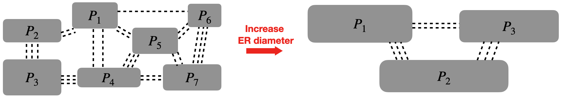
Figure 7: Graph decomposition results with respect to effective-resistance (ER) diameter

The graph decomposition results with respect to effective-resistance (ER) diameter are illustrated in Figure 7. The figure demonstrates that selecting a larger ER diameter leads to the decomposition of the graph into a smaller number of partitions, with more nodes included in each cluster. On the left side of the figure, the graph is decomposed into seven partitions: $P_{1},...,P_{7}$, by choosing a smaller ER diameter. Conversely, increasing the ER diameter on the right side of the figure results in the graph being partitioned into three clusters: $P_{1},P_{2},$ and $P_{3}$.

Appendix E Additional Results for GNN Stability Evaluation and Statistics of Datasets

We present the additional results in Figure 8, Figure 9, Figure 10, and Table 7. Table 6 summarizes the datasets utilized.

Table 6: Nettack adversarial attack targeting selected Cora samples in GCN

Nettack Level	Cosine Similarities: Stable/Unstable
1	0.99/0.90
2	0.98/0.84
3	0.97/0.81

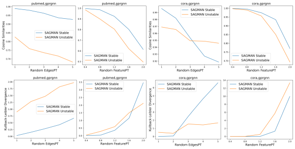
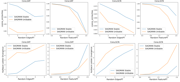
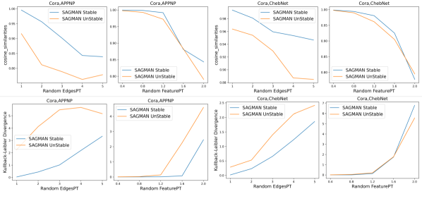
Figure 8: Figures represent cosine similarities and KL divergence. ”Random EdgesPT” corresponds to the DICE edge evasion attack. ”Random FeaturePT” refers to Gaussian noise evasion perturbation $X+\xi\eta$, where $X$ is feature matrix, $\eta$ is Gaussian noise, $\xi$ is noise level controls

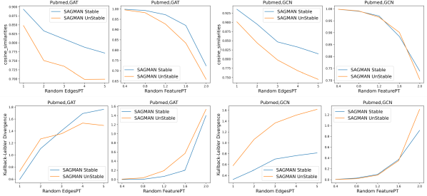
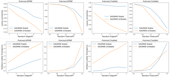
Figure 9: The horizontal axes, denoted by $X$, represent the magnitude of perturbation applied. ‘Random EdgesPT’ refers to the DICE adversarial attack scenario, in which pairs of nodes with different labels are connected and pairs with the same label are disconnected, with the number of pairs being equal to $X$. ‘Random FeaturePT’ indicates the application of Gaussian noise perturbation, expressed as $FM+X\eta$, where $FM$ denotes the feature matrix and $\eta$ represents Gaussian noise. The upper and lower subfigures illustrate the cosine similarity and the Kullback–Leibler Divergence (KLD). ‘SAGMAN Stable/Unstable’ denotes the samples that are classified as stable or unstable by SAGMAN, respectively.

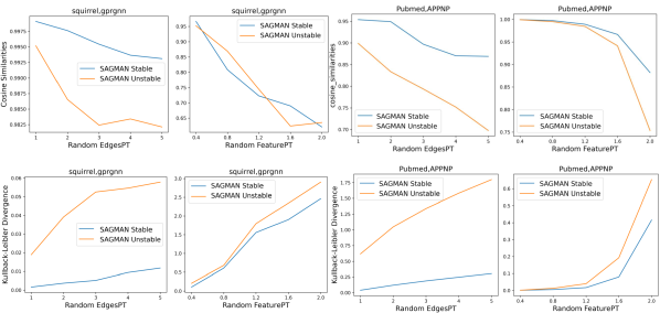
Figure 10: The horizontal axes, denoted by $X$, represent the magnitude of perturbation applied. ‘Random EdgesPT’ refers to the DICE adversarial attack scenario, in which pairs of nodes with different labels are connected and pairs with the same label are disconnected, with the number of pairs being equal to $X$. ‘Random FeaturePT’ indicates the application of Gaussian noise perturbation, expressed as $FM+X\eta$, where $FM$ denotes the feature matrix and $\eta$ represents Gaussian noise. The upper and lower subfigures illustrate the cosine similarity and the Kullback–Leibler Divergence (KLD). ‘SAGMAN Stable/Unstable’ denotes the samples that are classified as stable or unstable by SAGMAN, respectively.

Table 7: Summary of datasets used in our experiments

Dataset	Type	Nodes	Edges	Classes	Features
Cora	Homophily	2,485	5,069	7	1,433
Cora-ML	Homophily	2,810	7,981	7	2,879
Pubmed	Homophily	19,717	44,324	3	500
Citeseer	Homophily	2,110	3,668	6	3,703
Chameleon	Heterophily	2,277	62,792	5	2,325
Squirrel	Heterophily	5,201	396,846	5	2,089
ogbn-arxiv	Homophily	169,343	1,166,243	40	128

Appendix F Why Generalized Eigenpairs Associate with DMD

Cheng et al. propose a method to estimate the maximum distance mapping distortion (DMD), denoted as $\delta^{M}_{max}$, by solving the following combinatorial optimization problem:

$$\max{\delta^{M}}=\mathop{\max_{\forall p,q\in V}}_{p\neq q}\frac{e_{p,q}^{\top}L_{Y}^{+}e_{p,q}}{e_{p,q}^{\top}L_{X}^{+}e_{p,q}}$$ (16)

When computing $\delta^{M}_{max}$ via effective-resistance distance, the stability score is an upper bound of $\delta^{M}_{max}$ (Cheng et al., 2021).

A function $Y=M(X)$ is called Lipschitz continuous if there exists a real constant $K\geq 0$ such that for all $x_{i}$, $x_{j}\in X$:

$$dist_{Y}(M(x_{i}),M(x_{j}))\leq Kdist_{X}(x_{i},x_{j}),$$ (17)

where $K$ is the Lipschitz constant for the function $M$. The smallest Lipschitz constant, denoted by $K^{*}$, is called the best Lipschitz constant. Let the resistance distance be the distance metric, then (Cheng et al., 2021):

$$\lambda_{max}(L_{Y}^{+}L_{X})\geq K^{*}\geq\delta^{M}_{max}.$$ (18)

Equation 18 indicates that the $\lambda_{max}(L_{Y}^{+}L_{X})$ is also an upper bound of the best Lipschitz constant $K^{*}$ under the low dimensional manifold setting. A greater $\lambda_{max}(L_{Y}^{+}L_{X})$ of a function (model) implies worse stability since the output will be more sensitive to small input perturbations. A node pair $(p,q)$ is deemed non-robust if it exhibits a large DMD, i.e., $\delta^{M}(p,q)\approx\delta^{M}_{\max}$. This suggests that a non-robust node pair consists of nodes that are adjacent in the $G_{X}$ but distant in the $G_{Y}$. To effectively identify such non-robust node pairs, the Cut Mapping Distortion (CMD) metric was introduced. For two graphs $G_{X}$ and $G_{Y}$ sharing the same node set $V$, let $S\subset V$ denote a node subset and $\bar{S}$ denote its complement. Also, let $cut_{G}(S,\bar{S})$ denote the number of edges crossing $S$ and $\bar{S}$ in graph $G$. The CMD $\zeta(S)$ of node subset $S$ is defined as (Cheng et al., 2021):

$$\zeta(S)\overset{\mathrm{def}}{=}\frac{cut_{G_{Y}}(S,\bar{S})}{cut_{G_{X}}(S,\bar{S})}.$$ (19)

A small CMD score indicates that node pairs crossing the boundary of $S$ are likely to have small distances in $G_{X}$ but large distances in $G_{Y}$.

Given the Laplacian matrices $L_{X}$ and $L_{Y}$ of input and output graphs, respectively, the minimum CMD $\zeta_{\min}$ satisfies the following inequality:

$$\zeta_{\min}=\mathop{\min_{\forall S\subset V}}\zeta(S)\geq\frac{1}{\sigma_{\max}(L_{Y}^{+}L_{X})}$$ (20)

Equation 20 establishes a connection between the maximum generalized eigenvalue $\sigma_{\max}(L_{Y}^{+}L_{X})$ and $\zeta_{\min}$, indicating the ability to exploit the largest generalized eigenvalues and their corresponding eigenvectors to measure the stability of node pairs. Embedding $G_{X}$ with generalized eigenpairs. We first compute the weighted eigensubspace matrix $V_{s}\in{\mathbb{R}^{N\times s}}$ for spectral embedding on $G_{X}$ with $N$ nodes:

$$V_{s}\overset{\mathrm{def}}{=}\left[{v_{1}}{\sqrt{\sigma_{1}}},...,{v_{s}}{\sqrt{\sigma_{s}}}\right],$$ (21)

where $\sigma_{1},\sigma_{2},...,\sigma_{s}$ represent the first $s$ largest eigenvalues of $L_{Y}^{+}L_{X}$ and $v_{1},v_{2},...,v_{s}$ are the corresponding eigenvectors. Consequently, the input graph $G_{X}$ can be embedded using $V_{s}$, so each node is associated with an $s$-dimensional embedding vector. We can then quantify the stability of an edge $(p,q)\in E_{X}$ by measuring the spectral embedding distance of its two end nodes $p$ and $q$. Formally, we have the edge stability score defined for any edge $(p,q)\in E_{X}$ as $stability^{M}(p,q)\overset{\mathrm{def}}{=}\|V_{s}^{\top}e_{p,q}\|_{2}^{2}$ Let $u_{1},u_{2},...,u_{s}$ denote the first $s$ dominant generalized eigenvectors of $L_{X}L_{Y}^{+}$. If an edge $(p,q)$ is dominantly aligned with one dominant eigenvector $u_{k}$, where $1\leq k\leq r$, the following holds:

$$(u^{\top}_{i}e_{p,q})^{2}\approx\begin{cases}\alpha_{k}^{2}\gg 0&\text{ if }(i=k)\\ 0&\text{ if }(i\neq k).\end{cases}$$ (22)

Then its edge stability score has the following connection with its DMD computed using effective-resistance distances (Cheng et al., 2021):

$$\|V_{s}^{\top}e_{p,q}\|_{2}^{2}\propto\left(\delta^{M}(p,q)\right)^{3}.$$ (23)

The stability score of an edge $(p,q)\in E_{X}$ can be regarded as a surrogate for the directional derivative $\|\nabla_{v}M(x)\|$ under the manifold setting, where $v=\pm(x_{p}-x_{q})$. An edge with a larger stability score is considered more non-robust and can be more vulnerable to attacks along the directions formed by its end nodes.

Last, the node stability score can be calculated for any node (data sample) $p\in V$ as follows:

$$score(p)=\frac{1}{|\mathbb{N}_{X}(p)|}\sum_{q_{i}\in\mathbb{N}_{X}(p)}\left(\|V_{s}^{\top}e_{p,q}\|^{2}_{2})\right)\propto\frac{1}{|\mathbb{N}_{X}(p)|}\sum_{q_{i}\in\mathbb{N}_{X}(p)}\left(\delta^{M}(p,q_{i})\right)^{3}$$ (24)

where $q_{i}\in\mathbb{N}_{X}(p)$ denotes the $i$-th neighbor of node $p$ in graph $G_{X}$, and $\mathbb{N}_{X}(p)\in V$ denotes the node set including all the neighbors of $p$. The DMD score of a node (data sample) $p$ can be regarded as a surrogate for the function gradient $\|\nabla_{x}M(p)\|$ where $x$ is near $p$ under the manifold setting. A node with a larger stability score implies it is likely more vulnerable to adversarial attacks.

In this study, we restrict our calculations of stability scores to the two largest generalized eigenpairs. We also show results of the third and fourth largest generalized eigenpairs, as well as the fifth and sixth largest generalized eigenpairs in Table 8.

Table 8: Cosine Similarity and KL Divergence for DICE Edges Perturbation and Random Feature Perturbation. We bold the better results.

		Largest Generalized Eigenpairs: 1st and 2nd/3rd and 4th/5th and 6th
Method	PT Level	Cosine		KL Divergence
		Stable	Unstable	Stable	Unstable
EdgesPT	1	0.99/0.98/0.99	0.97/0.96/0.91	0.04/0.25/0.12	0.46/0.73/1.83
EdgesPT	2	0.96/0.87/0.96	0.92/0.89/0.86	0.82/1.17/1.11	2.43/2.01/3.47
EdgesPT	3	0.88/0.81/0.90	0.92/0.87/0.84	2.18/2.29/2.04	2.71/3.79/5.34
EdgesPT	4	0.83/0.80/0.85	0.88/0.85/0.85	4.57/3.29/3.83	4.16/4.23/5.25
EdgesPT	5	0.81/0.78/0.82	0.88/0.83/0.76	3.88/4.56/5.28	4.92/4.07/6.02
FeaturePT	0.4	1.00/0.84/0.81	1.00/0.75/0.68	0.00/2.16/5.70	0.00/4.57/8.24
FeaturePT	0.8	1.00/0.79/0.75	1.00/0.73/0.71	0.00/4.00/6.49	0.01/4.87/8.29
FeaturePT	1.2	0.98/0.78/0.76	0.98/0.70/0.69	0.02/6.11/6.65	0.08/5.47/9.33
FeaturePT	1.6	0.97/0.69/0.71	0.93/0.70/0.64	0.01/8.94/8.85	1.09/7.07/8.41
FeaturePT	2.0	0.80/0.67/0.70	0.82/0.72/0.66	1.72/8.57/9.53	4.02/5.45/9.40

Appendix G Various Sampling Schemes for SAGMAN-guided Perturbations

Previous works (Cheng et al., 2021; Hua et al., 2021; Chang et al., 2017) highlighted that only part of the dataset plays a crucial role in model stability, so we want to focus on the difference between the most ”stable” and ”unstable” parts. However, it is certainly feasible to evaluate the entire graph. Table 9 shows the result regarding the Pubmed dataset in GPRGNN under Gaussian noise perturbation. Samples were segmented based on SAGMAN ranking, with the bottom 20% being the most ”stable”, the middle 60% as intermediate, and the top 20% representing the most ”unstable”. As anticipated, the ”stable” category (representing the bottom 20%) should exhibit the lowest average KL divergences. This is followed by the intermediate category (covering the mid 60%), and finally, the ”unstable” category (comprising the top 20%) should display the highest divergences.

Table 9: KLD across varying Gaussian noise perturbations, expressed as $FM+X\eta$, where $FM$ denotes the feature matrix, $\eta$ represents Gaussian noise, and $X$ denotes the perturbation level. The dataset is divided into three segments based on the stability ranking of nodes as determined by SAGMAN.

Perturbation Level	KL divergence (bottom 20%)	KL divergence (mid 60%)	KL divergence (top 20%)
0.4	0.01	0.03	0.03
0.8	0.09	0.16	0.19
1.2	0.43	0.56	0.59

References

- Belkin & Niyogi (2003) Belkin, M. and Niyogi, P. Laplacian eigenmaps for dimensionality reduction and data representation. Neural computation, 15(6):1373–1396, 2003.
- Bojchevski & Günnemann (2019) Bojchevski, A. and Günnemann, S. Adversarial attacks on node embeddings via graph poisoning. In International Conference on Machine Learning, pp. 695–704. PMLR, 2019.
- Bruna et al. (2013) Bruna, J., Zaremba, W., Szlam, A., and LeCun, Y. Spectral networks and locally connected networks on graphs. arXiv preprint arXiv:1312.6203, 2013.
- Chang et al. (2017) Chang, H.-S., Learned-Miller, E., and McCallum, A. Active bias: Training more accurate neural networks by emphasizing high variance samples. Advances in Neural Information Processing Systems, 30, 2017.
- Chen et al. (2018) Chen, J., Wu, Y., Xu, X., Chen, Y., Zheng, H., and Xuan, Q. Fast gradient attack on network embedding. arXiv preprint arXiv:1809.02797, 2018.
- Cheng et al. (2021) Cheng, W., Deng, C., Zhao, Z., Cai, Y., Zhang, Z., and Feng, Z. Spade: A spectral method for black-box adversarial robustness evaluation. In International Conference on Machine Learning, pp. 1814–1824. PMLR, 2021.
- Chien et al. (2020) Chien, E., Peng, J., Li, P., and Milenkovic, O. Adaptive universal generalized pagerank graph neural network. arXiv preprint arXiv:2006.07988, 2020.
- Chu et al. (2020) Chu, T., Gao, Y., Peng, R., Sachdeva, S., Sawlani, S., and Wang, J. Graph sparsification, spectral sketches, and faster resistance computation via short cycle decompositions. SIAM Journal on Computing, (0):FOCS18–85, 2020.
- Chung (1997) Chung, F. R. Spectral graph theory, volume 92. American Mathematical Soc., 1997.
- Cucuringu et al. (2016) Cucuringu, M., Koutis, I., Chawla, S., Miller, G., and Peng, R. Simple and scalable constrained clustering: a generalized spectral method. In Artificial Intelligence and Statistics, pp. 445–454. PMLR, 2016.
- Defferrard et al. (2016) Defferrard, M., Bresson, X., and Vandergheynst, P. Convolutional neural networks on graphs with fast localized spectral filtering. Advances in neural information processing systems, 29, 2016.
- Deng et al. (2022) Deng, C., Li, X., Feng, Z., and Zhang, Z. Garnet: Reduced-rank topology learning for robust and scalable graph neural networks. arXiv preprint arXiv:2201.12741, 2022.
- Dong et al. (2019) Dong, X., Thanou, D., Rabbat, M., and Frossard, P. Learning graphs from data: A signal representation perspective. IEEE Signal Processing Magazine, 36(3):44–63, 2019.
- Erdös et al. (1965) Erdös, P., Harary, F., and Tutte, W. T. On the dimension of a graph. Mathematika, 12(2):118–122, 1965.
- Fan et al. (2019) Fan, W., Ma, Y., Li, Q., He, Y., Zhao, E., Tang, J., and Yin, D. Graph neural networks for social recommendation. In The world wide web conference, pp. 417–426, 2019.
- Feng (2021) Feng, Z. Sgl: Spectral graph learning from measurements. In 2021 58th ACM/IEEE Design Automation Conference (DAC), pp. 727–732. IEEE, 2021.
- Gama et al. (2020) Gama, F., Bruna, J., and Ribeiro, A. Stability properties of graph neural networks. IEEE Transactions on Signal Processing, 68:5680–5695, 2020.
- Gasteiger et al. (2018) Gasteiger, J., Bojchevski, A., and Günnemann, S. Predict then propagate: Graph neural networks meet personalized pagerank. arXiv preprint arXiv:1810.05997, 2018.
- Golub & Van Loan (2013) Golub, G. H. and Van Loan, C. F. Matrix computations, volume 3. JHU press, 2013.
- Grover & Leskovec (2016) Grover, A. and Leskovec, J. node2vec: Scalable feature learning for networks. In Proceedings of the 22nd ACM SIGKDD international conference on Knowledge discovery and data mining, pp. 855–864, 2016.
- Harper & Konstan (2015) Harper, F. M. and Konstan, J. A. The movielens datasets: History and context. Acm transactions on interactive intelligent systems (tiis), 5(4):1–19, 2015.
- Hu et al. (2020) Hu, Z., Dong, Y., Wang, K., Chang, K.-W., and Sun, Y. Gpt-gnn: Generative pre-training of graph neural networks. In Proceedings of the 26th ACM SIGKDD International Conference on Knowledge Discovery & Data Mining, pp. 1857–1867, 2020.
- Hua et al. (2021) Hua, W., Zhang, Y., Guo, C., Zhang, Z., and Suh, G. E. Bullettrain: Accelerating robust neural network training via boundary example mining. Advances in Neural Information Processing Systems, 34:18527–18538, 2021.
- Jin et al. (2020) Jin, W., Li, Y., Xu, H., Wang, Y., and Tang, J. Adversarial attacks and defenses on graphs: A review and empirical study. arXiv preprint arXiv:2003.00653, 10(3447556.3447566), 2020.
- Jin et al. (2021) Jin, W., Li, Y., Xu, H., Wang, Y., Ji, S., Aggarwal, C., and Tang, J. Adversarial attacks and defenses on graphs. ACM SIGKDD Explorations Newsletter, 22(2):19–34, 2021.
- Keisler (2022) Keisler, R. Forecasting global weather with graph neural networks. arXiv preprint arXiv:2202.07575, 2022.
- Kenlay et al. (2021) Kenlay, H., Thanou, D., and Dong, X. Interpretable stability bounds for spectral graph filters. In International conference on machine learning, pp. 5388–5397. PMLR, 2021.
- Keriven et al. (2020) Keriven, N., Bietti, A., and Vaiter, S. Convergence and stability of graph convolutional networks on large random graphs. Advances in Neural Information Processing Systems, 33:21512–21523, 2020.
- Kipf & Welling (2016) Kipf, T. N. and Welling, M. Semi-supervised classification with graph convolutional networks. arXiv preprint arXiv:1609.02907, 2016.
- Koutis et al. (2010) Koutis, I., Miller, G. L., and Peng, R. Approaching optimality for solving sdd linear systems. In Foundations of Computer Science (FOCS), 2010 51st Annual IEEE Symposium on, pp. 235–244. IEEE, 2010.
- Liu et al. (2019) Liu, Y. P., Sachdeva, S., and Yu, Z. Short cycles via low-diameter decompositions. In Proceedings of the Thirtieth Annual ACM-SIAM Symposium on Discrete Algorithms, pp. 2602–2615. SIAM, 2019.
- Malkov & Yashunin (2018) Malkov, Y. A. and Yashunin, D. A. Efficient and robust approximate nearest neighbor search using hierarchical navigable small world graphs. IEEE transactions on pattern analysis and machine intelligence, 42(4):824–836, 2018.
- Mirhoseini et al. (2021) Mirhoseini, A., Goldie, A., Yazgan, M., Jiang, J. W., Songhori, E., Wang, S., Lee, Y.-J., Johnson, E., Pathak, O., Nazi, A., et al. A graph placement methodology for fast chip design. Nature, 594(7862):207–212, 2021.
- Ng et al. (2001) Ng, A., Jordan, M., and Weiss, Y. On spectral clustering: Analysis and an algorithm. Advances in neural information processing systems, 14, 2001.
- Peng et al. (2015) Peng, R., Sun, H., and Zanetti, L. Partitioning well-clustered graphs: Spectral clustering works! In Conference on learning theory, pp. 1423–1455. PMLR, 2015.
- Roldán & Parrondo (2012) Roldán, É. and Parrondo, J. M. Entropy production and kullback-leibler divergence between stationary trajectories of discrete systems. Physical Review E, 85(3):031129, 2012.
- Roy et al. (2009) Roy, S., Lane, T., and Werner-Washburne, M. Learning structurally consistent undirected probabilistic graphical models. In Proceedings of the 26th annual international conference on machine learning, pp. 905–912, 2009.
- Schaefer (2012) Schaefer, M. Realizability of graphs and linkages. In Thirty Essays on Geometric Graph Theory, pp. 461–482. Springer, 2012.
- Spielman & Srivastava (2008) Spielman, D. A. and Srivastava, N. Graph sparsification by effective resistances. In Proceedings of the fortieth annual ACM symposium on Theory of computing, pp. 563–568, 2008.
- Spielman & Teng (2011) Spielman, D. A. and Teng, S.-H. Spectral sparsification of graphs. SIAM Journal on Computing, 40(4):981–1025, 2011.
- Sun et al. (2020) Sun, Y., Wang, S., Tang, X., Hsieh, T.-Y., and Honavar, V. Adversarial attacks on graph neural networks via node injections: A hierarchical reinforcement learning approach. In Proceedings of the Web Conference 2020, pp. 673–683, 2020.
- Szegedy et al. (2013) Szegedy, C., Zaremba, W., Sutskever, I., Bruna, J., Erhan, D., Goodfellow, I., and Fergus, R. Intriguing properties of neural networks. arXiv preprint arXiv:1312.6199, 2013.
- Veličković et al. (2017) Veličković, P., Cucurull, G., Casanova, A., Romero, A., Lio, P., and Bengio, Y. Graph attention networks. arXiv preprint arXiv:1710.10903, 2017.
- Waniek et al. (2018) Waniek, M., Michalak, T. P., Wooldridge, M. J., and Rahwan, T. Hiding individuals and communities in a social network. Nature Human Behaviour, 2(2):139–147, 2018.
- Xu et al. (2019) Xu, K., Chen, H., Liu, S., Chen, P.-Y., Weng, T.-W., Hong, M., and Lin, X. Topology attack and defense for graph neural networks: An optimization perspective. arXiv preprint arXiv:1906.04214, 2019.
- Yao et al. (2019) Yao, L., Mao, C., and Luo, Y. Graph convolutional networks for text classification. In Proceedings of the AAAI conference on artificial intelligence, volume 33, pp. 7370–7377, 2019.
- Ying et al. (2018) Ying, R., He, R., Chen, K., Eksombatchai, P., Hamilton, W. L., and Leskovec, J. Graph convolutional neural networks for web-scale recommender systems. In Proceedings of the 24th ACM SIGKDD international conference on knowledge discovery & data mining, pp. 974–983, 2018.
- Yu et al. (2017) Yu, B., Yin, H., and Zhu, Z. Spatio-temporal graph convolutional networks: A deep learning framework for traffic forecasting. arXiv preprint arXiv:1709.04875, 2017.
- Zhang et al. (2022) Zhang, Y., Zhao, Z., and Feng, Z. Sf-sgl: Solver-free spectral graph learning from linear measurements. IEEE Transactions on Computer-Aided Design of Integrated Circuits and Systems, 2022.
- Zhao et al. (2021) Zhao, Z., Zhang, Y., and Feng, Z. Towards scalable spectral embedding and data visualization via spectral coarsening. In Proceedings of the 14th ACM International Conference on Web Search and Data Mining, pp. 869–877, 2021.
- Zhou et al. (2020) Zhou, J., Cui, G., Hu, S., Zhang, Z., Yang, C., Liu, Z., Wang, L., Li, C., and Sun, M. Graph neural networks: A review of methods and applications. AI open, 1:57–81, 2020.
- Zhu et al. (2019) Zhu, D., Zhang, Z., Cui, P., and Zhu, W. Robust graph convolutional networks against adversarial attacks. In Proceedings of the 25th ACM SIGKDD international conference on knowledge discovery & data mining, pp. 1399–1407, 2019.
- Zügner et al. (2018) Zügner, D., Akbarnejad, A., and Günnemann, S. Adversarial attacks on neural networks for graph data. In Proceedings of the 24th ACM SIGKDD international conference on knowledge discovery & data mining, pp. 2847–2856, 2018.