Fairness Auditing with Multi-Agent Collaboration

Abstract

Existing work in fairness audits assumes that agents operate independently. In this paper, we consider the case of multiple agents auditing the same platform for different tasks. Agents have two levers: their collaboration strategy, with or without coordination beforehand, and their sampling method. We theoretically study their interplay when agents operate independently or collaborate. We prove that, surprisingly, coordination can sometimes be detrimental to audit accuracy, whereas uncoordinated collaboration generally yields good results. Experimentation on real-world datasets confirms this observation, as the audit accuracy of uncoordinated collaboration matches that of collaborative optimal sampling.

1 Introduction

ML models are becoming integral to many business and industrial processes, increasingly impacting several facets of our lives (Holstein et al., 2019). Such models are increasingly employed to drive decisions in high-stakes domains (Buyl & De Bie, 2024). For example, many financial institutions use AI-driven models where various attributes such as income, credit score, and employment history influence a decision on whether a particular loan is issued (Mhlanga, 2021). These models are also used to automate the hiring process of particular companies, which would otherwise be labor-intensive (Giang, 2018; Hunkenschroer & Luetge, 2022). As these models may significantly impact people’s lives, their fairness and regulatory compliance have become increasingly important (Pessach & Shmueli, 2022; Le Merrer et al., 2023).

Estimating the fairness of machine learning (ML) models is commonly done through algorithmic audits by regulatory bodies (Ng, 2021). Auditors, however, usually are not granted unrestricted access to an ML model to protect intellectual property but instead send queries to the model and use the query responses (that is, a black-box interaction) to detect fairness violations, biases or improper data usage. For instance, (Rastegarpanah et al., 2021) proposes to study the illegal use of some profile data in the response of a model in such a query-response setup. Yet, as of today, an auditor performs her audit tasks on each attribute of interest sequentially, one after the other, and independent of other auditors. For example, when she wants to audit an ML model that predicts whether it is safe to issue a loan (Feldman et al., 2015), she begins by auditing the fairness property of the gender attribute and then independently audits the fairness property on the race attribute in a subsequent task. While collaboration in a single task has recently been introduced in the community (Xu et al., 2023), collaborative auditing for multiple tasks has not been studied to the best of our knowledge. Moreover, existing works on algorithmic audits assume that each auditor has a cap on the number of queries they can send to the platform (Neiswanger et al., 2021; Yan & Zhang, 2022; Rastegarpanah et al., 2021) to prevent the overloading of the service. Therefore, we ask the question: can auditors benefit from collaboration among individual audit tasks, e.g., by strategically constructing and sharing queries and responses?

We answer affirmatively by studying the collaboration strategies and sampling methods of independent agents representing an auditor, each focusing on a different attribute in a common auditing process. More specifically, we consider settings in which agents collaborate to increase the efficiency and accuracy of the overall auditing process. Specifically, we consider a setting where auditors are interested in determining the demographic parity (DP) of a model on specific attributes. DP is a crucial fairness property in fairness studies (Yan & Zhang, 2022; Singh & Chunara, 2023; Pessach & Shmueli, 2022).

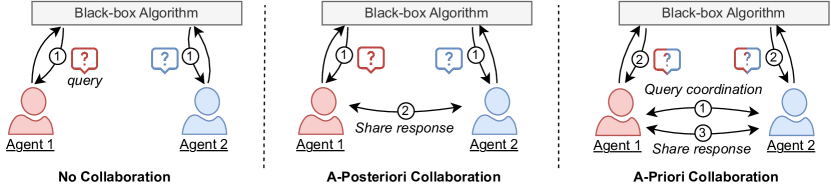
Figure 1: This work analyses collaboration strategies of an auditor with her two agents: no collaboration (left figure, baseline), a-posteriori collaboration where agents share query responses (middle figure), and a-priori collaboration where agents additionally coordinate on queries to be sent (right figure).

This paper introduces and analyses two realistic forms of multi-agent collaboration for fairness audits. In the a-posteriori collaboration, agents share both their queries and the query responses they receive among each other. In the a-priori collaboration, in addition, agents coordinate beforehand on their queries to maximize the information that can be gathered. Figure 1 visualizes the workflow of two agents, without collaboration (left) and with two different collaboration strategies (middle and right).

This work makes the following contributions:

• We study a multi-agent setup that enables agents to collaboratively conduct fairness audits of ML models (Section 3 and 4). The collaborations are driven using coordinated sampling methods on sensitive attributes under audit and by sharing query responses among agents.

• We provide a theoretical analysis of the a-priori and a-posteriori collaboration strategies (Section 5). We derive that the estimation error of the DP of both a-posteriori and a-priori collaboration scales in $\Theta(1/\sqrt{m})$, where $m$ is the number of collaborative agents. This is surprising, as one could have expected that the relative independence of the a-posteriori strategy would lead to a worse performance than a-priori; we formally prove this.

• Using three large real-world fairness datasets (German Credit, Propublica, and Folktables), we empirically demonstrate the benefits of collaboration over non-collaborative audits, as well as exhibiting the performance gap favorable to the a-posteriori strategy (Section 6). We compare it to an optimal (yet impractical) sampling method and observe their quasi-overlap in performance.

2 Preliminaries

We first formalize the audit process and then introduce the fairness metric that we focus on in this work.

Auditing Fairness. We consider a black-box algorithm $\mathcal{A}$ (, a ML model) at the platform:

$$\mathcal{A}:\mathcal{X}\mapsto\{0,1\},$$

where the input space $\mathcal{X}$ contains independent protected attributes $X_{1},\dots,X_{m}$ and $\mathcal{A}$ outputs a binary response $Y$. $m$ different agents $A_{1},\dots,A_{m}$ query the same black-box algorithm $\mathcal{A}$ to audit fairness properties of specific attributes. Specifically, each agent $A_{i}$ focuses on evaluating a protected attribute $X_{i}$. For example, in a loan attribution application (Feldman et al., 2015), some agent $A_{1}$ could audit a fairness property of the gender attribute ($X_{1}$) and $A_{2}$ could audit a fairness property on the race attribute ($X_{2}$). Each attribute $X_{i}$ induces two groups in $X$ (the favored and unfavored groups). We call a stratum each intersection of these $2m$ groups: there are $2^{m}$ strata.

In line with related work in this domain, we assume that each auditor can issue a fixed total number of queries $B$ (Yan & Zhang, 2022). We refer to $B$ as the query budget. We assume that each agent of a particular auditor can send $R$ queries to $\mathcal{A}$ where $R=B/m$ is the per-agent query budget.

Fairness Metric. There is a wide range of definitions for fairness and bias in the existing literature (Saleiro et al., 2018). DP, denoted as $D$, has emerged as a critical fairness metric for modeling social equality (Mouzannar et al., 2019). A black-box algorithm satisfies demographic parity when it, on average, delivers the same predictions across different protected groups. Despite its simplicity, $D$ is a key measure for fairness, especially in high-stakes areas such as finance and recruitment, where decisions can significantly impact individuals’ lives. EU regulations also recognize $D$ as a metric for detecting bias in algorithmic decision-making systems (EU, 2022).

Definition 2.1.

The demographic parity $D_{i}$ with respect to some binary protected attribute $X_{i}$ captures the impact of $X_{i}$ on a prediction $Y$:

$$D_{i}=\mathds{P}(Y=1|X_{i}=1)-\mathds{P}(Y=1|X_{i}=0)$$ (1)

Agent $A_{i}$ can use her $R$ queries to estimate DP on protected attribute $X_{i}$ by querying any $x\in\mathcal{X}$. Let $\hat{D}_{i}$ be a DP estimator:

$$\hat{D}_{i}=\mathds{\hat{P}}(Y=1|X_{i}=1)-\mathds{\hat{P}}(Y=1|X_{i}=0)$$ (2)

For brevity, we will write $\hat{Y}_{i}=\mathds{\hat{P}}(Y=1|X_{i}=1)$ and $\hat{Y}_{\bar{i}}=\mathds{\hat{P}}(Y=1|X_{i}=0)$.

According to the Digital Services Act (European Commission, 2020) among others, if $D_{i}=0\pm 0.2$, then $\mathcal{A}$ respects demographic parity on protected attribute $X_{i}$. While demographic parity could, in addition, be estimated relatively to each stratum (as in intersectional fairness (Gohar & Cheng, 2023)), we only focus in this paper on attribute-level DP.

Objective of an Auditor. The goal of each auditor is to audit as accurately as possible, , by obtaining DP estimations that are close to the ground truth DPs. An auditor might be interested in multiple DP estimations for different attributes. We consider that all obtained estimations are equally valuable for the auditor. Therefore, we consider that the auditor’s goal is to have the average of DP errors, , the difference between its estimated DPs and the actual DPs, as small as possible. The choice of a regular average as the metric is arbitrary, acknowledging that alternative metrics exist. For instance, Xu et al. (2023) proposes a metric ensuring fairness between agents. However, in our context, where all agents share the common goal of auditing, this paper strives for the lowest averaged error.

A Running Illustrative Example. Throughout this work, we use an illustrative example to structure the explanation of auditing and our collaboration strategies. We assume two agents ($m=2$) that audit black-box algorithm $\mathcal{A}$ whose input space consists of two attributes: gender (whether someone is male or not) and disability (whether someone has a disability or not). $A_{1}$ and $A_{0}$ are interested in estimating the $D$ of the gender ($X_{1}$) and disability ($X_{2}$) attributes, respectively. We also model the real-world distributions of the gender attribute as $51\%$ male and $49\%$ female, and the disabled attribute as $2\%$ of the population having a disability and $98\%$ not. For instance, if $Y_{\bar{1}}=0$ (i.e. no women receive a positive response) and $Y_{1}=0.1$, then $D_{1}=0.1$ so $\mathcal{A}$ is fair on gender attribute $X_{1}$.

3 Collaboration Strategies and Sampling

An agent relies on: (i) a collaboration strategy with other agents, and (ii) a sampling method that influences the way she constructs her queries. We introduce our collaboration strategies and sampling methods next.

3.1 Collaboration Strategies

We begin by introducing two natural collaboration strategies in a black-box audit context, along with a baseline approach that does not involve collaboration. These two strategies are also visualized in the middle and right of Figure 1.

a-posteriori Collaboration. The most natural collaboration scheme involves sharing queries and their responses among agents. In this approach, each agent independently queries the black-box algorithm and then shares the queries and resulting responses with the other agents so that all agents can access a pooled set of queries.

a-priori Collaboration. We introduce a second collaborative strategy, aiming at a preliminary coordination of agents. With a-priori collaboration, agents collectively implement a sampling strategy (detailed in the next subsection), accounting for the tasks and objectives of the other participating agents. More specifically, all agents divide the input space into $2^{m}$ strata and agree on the sampling strategy of each stratum. This coordination allows for a more integrated and strategic approach to querying, intending to enhance the overall effectiveness of the collaboration.

No Collaboration (baseline). To quantify the effectiveness of our collaboration strategies, we also consider a non-collaborative setting where each agent queries the black-box algorithm by itself and independently of the others. This baseline is also used in (Xu et al., 2023).

3.2 Sampling Methods

When an auditor sends a query to the black-box algorithm, she must set her query attributes according to a sampling method. One can use many different sampling methods for auditing (Kloek & Van Dijk, 1978; Yan & Zhang, 2022). Classic sampling methods leverage knowledge of data known in advance by the auditor. We consider three distinct sampling methods, all evaluated in conjunction with the previously mentioned collaboration strategies.

Uniform Sampling. Uniform sampling is the most generic and common strategy for sampling attributes. With uniform sampling, the allocation of queries with $X_{i}=0$, respectively $X_{i}=1$, mirrors the real-world distribution of $X$ on $X_{i}$. In our illustrative example, an agent that uses uniform sampling, sets the attribute corresponding to disability to 1 ($X_{2}=1$) in $2\%$ of the queries while setting to 0 ($X_{2}=0$) in $98\%$ of them (also see Section A.1).

This proportionate allocation of queries might not provide a robust enough estimator for $D$, especially on imbalanced attributes. In our example, we only dedicate a relatively small number of queries to capturing disabled people, possibly reducing the accuracy of estimating $D$. If a minority stratum is subjected to unfair treatment and the responses of $\mathcal{A}$ exhibit significant variability, then the agent should consider a more efficient sampling method.

Stratified Sampling. Disproportionate stratified sampling has emerged as an alternative to estimate the DP under attribute imbalance (Arieska & Herdiani, 2018; Keramat & Kielbasa, 1998). In this approach, the sample size drawn from each stratum is not proportional to the stratum’s size. Instead, an equal amount of the budget is allocated to each stratum, namely $1/n$ of the budget on each stratum if there are $n$ strata. This can be viewed as a case of non-collaborative stratified sampling. It ensures that each stratum of a given attribute is adequately represented in the audit by an agent. For our illustrative example, that means that $50\%$ of queries by an agent are with $X_{2}=1$ (disability) and $50\%$ with $X_{2}=0$, irrespective of the real-world distribution (also see Section A.1).

Equally dividing the total queries among each stratum may not be a good strategy. In particular, in situations where protected attributes are unbalanced (, when $P(X_{i}=1)$ is close to $0$ or $1$), the resulting stratum may be of uneven size. This is amplified by the growth of strata: each additional auditor doubles the number of strata. Such a pathological situation is analysed in Section 5.

Neyman Sampling. Neyman sampling is an optimal sampling strategy that finds the optimal allocation of queries among strata to lower the DP estimation error (Mathew et al., 2013). However, its practical application is hindered by the requirement of knowing the values of the standard deviation of the responses on $Y$. This is an insurmountable challenge in real-world situations because it is equivalent to knowing in advance $\hat{Y}_{i}$ and $\hat{Y}_{\bar{i}}$ that the auditor wants to estimate. Combined with the a-priori collaboration strategy, Neyman sampling represents the optimal sampling strategy and acts as an upper bound for realistic sampling strategies.

In the remainder of this work, we assume that agents are homogeneous: they all use the same sampling and collaboration strategy. We leave the analysis of collaboration among heterogeneous auditors to future work.

Rationale. With these notions being exposed, we are now able to motivate the proposal of these two collaboration strategies as being the only strategies available in our black-box audit setup. There are only two ways to collaborate in a query/response based approach: before sending the queries, or after doing so. For sampling, while uniform is at hand and easy to implement, stratified is the best one auditors can do without extra knowledge of the black-box.

4 Standard Errors in Collaboration

The primary objective of each auditor is to use a budget of $R$ per-agent queries to derive an accurate estimator, $\hat{D}_{i}$, of the demographic parity, $D_{i}$, of their respective protected attribute $X_{i}$. Note that $\hat{D}_{i}$ is a random variable. Analyzing its distribution is key to understanding the characteristics of the different estimators that result from the various sampling and collaboration strategies employed.

As illustrated in Equation (2), the demographic parity, $\hat{D}_{i}$, is determined by comparing the two empirical probabilities ($\hat{Y}_{i}$ and $\hat{Y}_{\bar{i}}$). Each empirical probability $\hat{Y}_{i}$ is calculated as the proportion of positive responses collected from queries within the group of interest: $\hat{Y}_{i}=\frac{|X_{i}=1,Y=1|}{|X_{1}=1|}.$ Similarly empirical probability $\hat{Y}_{\bar{i}}$ is defined by replacing $X_{i}=1$ by $X_{i}=0$ in the previous equation. We target unbiased estimators: the higher the query budget $R$, the closer one might expect the estimators to be to their true values: $\forall i,\lim_{R\to\infty}\mathbb{E}(\hat{D}_{i})=D_{i}.$

Since $\hat{D}_{i}=\hat{Y}_{i}-\hat{Y}_{\bar{i}}$ (, two independent mean estimation problems), it is easy to see that for uniform sampling strategies, regardless of the collaboration, this unbiasedness is granted by the central limit theorem, as samples are independent and identically distributed (IID). This observation also holds for no collaboration and a-posteriori since attributes are independent.

For a-priori collaboration with stratified sampling and a-priori collaboration with Neyman sampling, agent $i$ biases her sampling to cover the other protected groups $j\neq i$ evenly; as a result, samples are IID only among strata sharing the same $m$ protected attribute values (same gender and disability for $m=2$). Each attribute estimator is computed as the weighted average of stratum estimators, with the weights being the relative size of the stratum within the attribute. We provide in Table 3 (in the appendix) the definition of $\hat{D_{i}}$ for each sampling method.

For sufficiently large query budgets $B$, the errors of the unbiased estimator are well described by a normal distribution: $\hat{D_{i}}-D_{i}\sim\mathcal{N}(0,\epsilon_{i}^{2})$, and the $\epsilon_{i}$ is the standard error that agents seek to minimise.

4.1 Standard Errors

In our scenario, as each agent estimates both $\hat{Y}_{i}$ and $\hat{Y}_{\bar{i}}$ to estimate $\hat{D}_{i}$, $\epsilon_{i}$ is the sum of standard errors on $\hat{Y}_{i}$ and $\hat{Y}_{\bar{i}}$:

Definition 4.1.

Error on demographic parity. Let $R_{i}$ the number of queries satisfying $X_{i}=1$ and $R_{\bar{i}}$ the number of queries satisfying $X_{i}=0$, then the error on the pooled demographic parity on $X_{i}$ is:

$$\epsilon(i)=\sqrt{\frac{\sigma_{i}^{2}}{R_{i}}}+\sqrt{\frac{\sigma_{\bar{i}}^{2}}{R_{\bar{i}}}},$$ (3)

where $\sigma_{i}$ the standard deviation of $Y_{i}$ and $\sigma_{\bar{i}}$ the standard deviation of $Y_{\bar{i}}$.

The values of $R_{i}$ depend on the sampling method and collaboration strategy, and are given in Table 4 (in the appendix). For instance, when a-posteriori collaboration is employed with the stratified sampling method, it follows that $\forall i,R_{i}=R/2+(m-1)P_{i}R$ with $P_{i}=P(X_{i}=1)$. This signifies that each agent $i$ splits her budget evenly between their two groups of interest: $X_{i}=1$ and $X_{i}=0$, while the queries shared by other agents are uniformly sampled.

To globally assess the interest of auditors collaboration, we rely on the average DP error realized by agents:

Definition 4.2.

Average DP error. Consider a set $I$ of collaborative agents where each agent $(A_{j})_{j\in I}$ audits a demographic parity $D_{i}$ with error $\epsilon_{i}$, then the average DP error is:

$$\epsilon(I)=\frac{1}{|I|}\sum_{i\in I}\epsilon(i).$$ (4)

4.2 The Neyman Allocation

As mentioned previously, the Neyman allocation represents the optimal distribution of queries among strata to minimize the error in the estimation of fairness. Thus, the Neyman allocation is an allocation $(R_{i})_{i\in I}$ such that all agents in $I$ are collaborating a-priori. In other words, when every agent does not collaborate or leverages a-posteriori, each agent individually aims to minimize (4) for $I=\{i\}$. However, the standard error on the audit is still  (4) for $I=\{1,\dots,M\}$ as all agents are estimating fairness for the auditor.

5 Theoretical Bounds on DP Errors

In the following section, we quantify the advantage of the a-posteriori and a-priori collaboration strategies in terms of averaged standard error. We assume that even if the collaborative strategy is not a-priori, each agent uses the same sampling method among uniform, stratified, or Neyman. We defer all proofs to Appendix B for presentation clarity.

5.1 Uniform Sampling

This is the simplest case to study; the error using uniform sampling satisfies the equality:

$$\epsilon_{a-priori}^{uniform}(I)=\epsilon_{a-posteriori}^{uniform}(I)=\frac{1}{\sqrt{m}}\epsilon_{nocollab.}^{uniform}(I).$$ (5)

This means that the error on the audit decreases by a factor of the square root of the number of collaborative agents (, for $4$ agents, the error is divided by $2$). We note that choosing uniform a-priori and uniform a-posteriori leads to the same error. One reason why the a-posteriori collaboration is competitive is that the number of queries for the audit increases compared to the budgets of non-collaborative agents.

For an accurate audit, it is important for agent $A_{i}$ studying $D_{i}$ to have a manageable error for both terms in Equation 3. Specifically, the skewed allocation of queries in attributes with uniform sampling exacerbates one of the error terms in the $D$ estimation in Equation 3, leading to a high error in the term related to the minority group.

5.2 Neyman Sampling

The standard error is not only influenced by the probability of belonging to a particular stratum. It also depends on the probability of observing a positive response within that stratum. In that light, priority in sampling should be given to strata characterized by the highest levels of uncertainty in their responses; this is what captures the optimal allocation strategy here.

By definition of the optimal allocation,

$$\epsilon_{a-priori}^{Neyman}(I)\leq\frac{1}{\sqrt{m}}\epsilon_{nocollab.}^{Neyman}(I)\leq\epsilon_{nocollab.}^{uniform}(I)$$ (6)

$$\text{and~{} ~{}}\epsilon_{a-posteriori}^{Neyman}(I)\leq\epsilon_{nocollab.}^{Neyman}(I).$$ (7)

These results are similar to those obtained with uniform sampling except that we have inequalities instead of equalities. This means that the error can be lower than if we just multiplied the budget of each agent by $m$, which is a desirable property.

We also show that with numerous agents, a-posteriori with Neyman sampling is similar to a-posteriori with uniform sampling:

$$\epsilon_{a-posteriori}^{Neyman}(I)\underset{m\rightarrow+\infty}{\sim}\epsilon_{a-posteriori}^{uniform}(I).$$ (8)

That is to say, the error on the audit decreases by a factor of the square root of the number of collaborative agents by using a-posteriori. By definition of the optimal allocation, even when not collaborating, the error is lower than with the uniform method. However, the interest in using the optimal allocation with the a-posteriori strategy is almost null. Intuitively, the $R$ optimal queries of the agent are flooded among the $(m-1)R$ uniform queries of the agent on this attribute.

5.3 Stratified Sampling

By allocating queries in a balanced manner, , $R/2$ with $X_{i}=1$ and $R/2$ with $X_{i}=0$ (irrespective of the real-world distribution), stratified sampling can lead to a more accurate and reliable estimation of $D$.

The following results show that having more agents collaborating benefits the auditing process, , collaboration helps. It is formalized and proved as followed. Adding $(m-1)R$ queries reduces errors:

$$\epsilon_{a-posteriori}^{stratified}(I)\leq\epsilon_{nocollab.}^{stratified}(I).$$ (9)

As established for Neyman sampling in Equation 8, there is an asymptotic equivalence between stratified a-posteriori and uniform a-posteriori with numerous agents:

$$\epsilon_{a-posteriori}^{stratified}(I)\underset{m\rightarrow+\infty}{\sim}\epsilon_{a-posteriori}^{uniform}(I).$$ (10)

The error using stratified a-priori might grow with the increase of the amount of auditors, particularly when an attribute distribution is very unbalanced.

If $\forall i,P_{i}>0.7$ then:

$$\epsilon_{a-priori}^{stratified}(I)\underset{m\rightarrow+\infty}{\rightarrow}+\infty.$$ (11)

The next result shows that when $\mathcal{A}$ is fair, the stratified and Neyman sampling methods yield similar outcomes for non-collaborating agents:

$$\epsilon_{nocollab.}^{stratified}(I)\underset{\mathcal{A}~{}fair}{=}\epsilon_{nocollab.}^{Neyman}(I)$$ (12)

It means that the optimal allocation is realized with stratified sampling, , non-collaborating agents can reach the minimal error without knowledge of the black-box.

Finally, the following result yields an interesting outcome for auditors, in frequent scenarios where attributes are not balanced (, disability or race): the error of stratified a-posteriori can be lower than that of stratified a-priori:

$$\exists\text{cases},\epsilon_{a-posteriori}^{stratified}(I)<\epsilon_{a-priori}^{stratified}(I).$$ (13)

Hence, our claim is that coordination can sometimes lead to worse outcomes than without coordination.

Summary.

Figure 2 describes the theoretical relations driving the interplay between collaboration strategies and sampling methods. Apart from pathological situations in stratified a-priori, collaborating is always beneficial. Without collaboration, stratified sampling yields quasi-optimal results if attributes are balanced. The benefits of this optimized sampling ultimately vanishes when a-posteriori collaboration is used with many auditors, as the sampling realized by auditors $j\neq i$ is uniform with respect to attribute $i$. Recall that the best possible sampling, Neyman a-priori, is unrealistic in our black-box setting as it assumes auditors exploit the complete knowledge of the target algorithm. Hence, the gap between realistic strategies like stratified a-posteriori and Neyman a-priori represents the cost of incomplete knowledge. The experiments in the next section aim to measure this gap in practice.

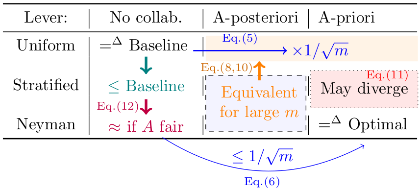
Figure 2: The influence of collaboration strategy and sampling method on the average DP error (summarizing our theoretical results).

6 Experiments and Results

To empirically evaluate and understand the gains of collaboration with real-world datasets, we implement a simulation framework in the Python 3 programming language. We leverage three datasets: German Credit (Hofmann, 1994), Propublica (Angwin et al., 2016) and Folktables (Ding et al., 2021) (full description is deferred to Appendix C). We consider five attributes on each dataset where each attribute is binary by default or binarized by following a certain scheme (see Appendix C). The labels for the prediction task in each dataset are also binary. To simulate black-box models, we adopt a unique strategy by treating dataset labels as responses from the ML model, avoiding the traditional need to train specific models for each audit task. This approach views datasets as extensive passive sampling sets of the target model, eliminating the need to select a training algorithm and an ML model from diverse choices. To ensure reproducibility, we open source all source code and documentation on GitHub.

Setup. We consider the uniform, stratified, and Neyman sampling methods, along with collaboration, a-posteriori collaboration, and a-priori collaboration strategies. The Folktables dataset is composed of $5\,916\,565$ samples. We run each experiment with the Folktables for $300$ repetitions. These repetitions yield a good balance between the accuracy of the mean and computational efficiency.

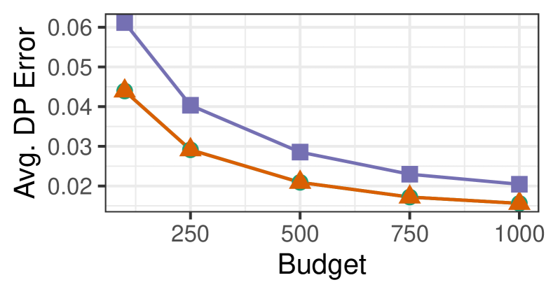
(a) Uniform Sampling

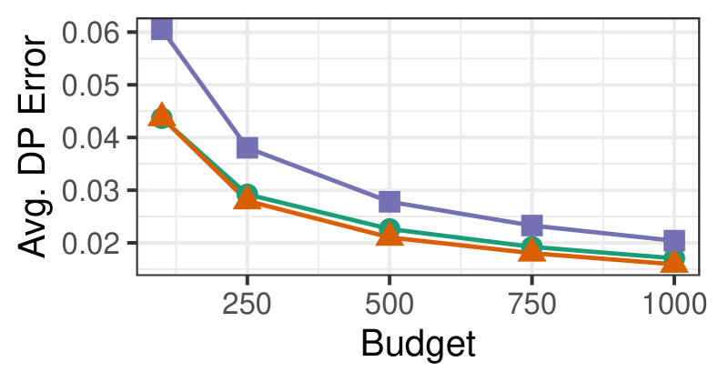
(b) Stratified Sampling

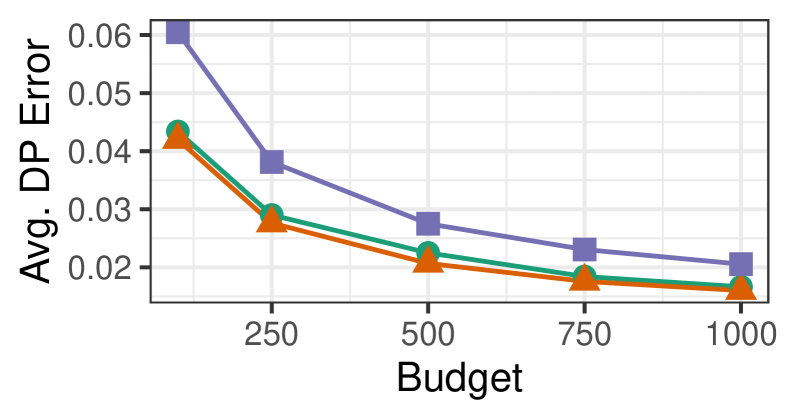
(c) Neyman Sampling

Figure 3: Average error on demographic parity (across agents) for different collaboration strategies and sampling methods, for the Folktables dataset. Results for the German Credit and Propublica datasets can be found in Section D.1.

6.1 Error of $\hat{D}$ for Two Agents and Increasing Budgets

We simulate the different collaboration strategies and sampling methods for all three datasets and observe the average error of the DP estimator $\hat{D}$ across agents for different per-agent query budgets $R$, ranging from $100$ to $1000$. For this experiment, two agents audit a particular attribute in each dataset; we consider age and marital status for the Folktables dataset. These results are shown in Figure 3 where each row represents a different dataset and each column, a different sampling method. Our first observation is that for all configurations, the average $\hat{D}$ error decreases as $R$ increases since individual $\hat{D}$ estimations become closer to the ground-truth value. Figure 3 also illustrates that a-posteriori or a-priori collaboration always decreases the average $\hat{D}$ error compared to when not collaborating and therefore it is always beneficial to collaborate.

Furthermore, under the same sampling method, the a-posteriori and a-priori collaborations perform similarly. As demonstrated by theory, these two strategies are equivalent when using uniform sampling. When comparing across sampling methods, we observe that at higher budgets, all strategies achieve similar error values. This is because as the budget rises, the estimations become more accurate, independent of the strategy. Consequently, all strategies will converge to the same final error value. At lower budgets, however, Neyman sampling performs better than uniform sampling. For example, at $R=100$, a-priori Neyman achieves an lower average error ($0.042$) than a-priori uniform ($0.044$). We observe similar behavior on the remaining two datasets, which results are included in Section D.1. Surprisingly, while Neyman sampling is always optimal, stratified sampling performs nearly as well, suggesting that the stratified allocation might not be as far from the Neyman optimal allocation when dealing with only two agents. We extend this comparison between strategies and collaborations in the next section, while considering more agents.

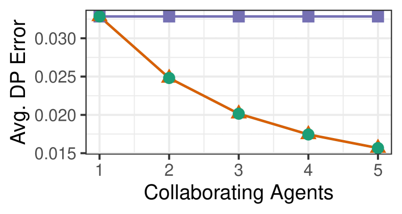
(a) Uniform Sampling

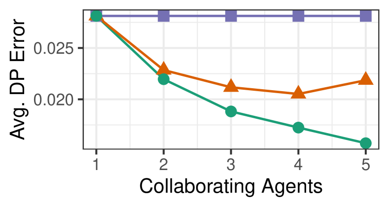
(b) Stratified Sampling

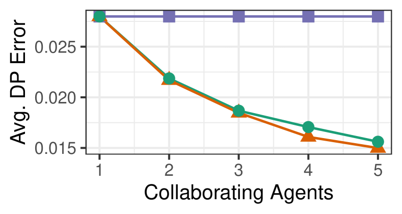
(c) Neyman Sampling

Figure 4: Average error on demographic parity with increasing number of collaborating agents for the Folktables dataset. Results for the German Credit and Propublica datasets can be found in Section D.2.

6.2 Error of $\hat{D}$ for Multiple Collaborating Agents

This experiment aims to observe how the average error of $\hat{D}$ changes as we increase the level of collaboration. For each dataset, we increase the number of collaborating agents ($m$) from $1$ (no collaboration) to $5$. When considering a particular $m$, we report the mean across all combinations of $m$ agent collaborations, for instance, all two agent combinations of protected attributes when $m=2$. Each combination is still run several times with different random seeds, as previously described. We set the budget $R=500$ for the Folktables dataset. Figure 4 visualizes our results where each column represents a different sampling method. The results for the remaining datasets are presented in Section D.2.

First, we observe that a-posteriori and a-priori are alike with uniform sampling, resulting in overlapping curves in Figure 4 (in line with theory). We observe that, in general, increasing $m$ decreases the average $\hat{D}$ error for collaborative strategies, while no collaboration achieves a constant error. Figure 4 shows that for the Neyman sampling, the a-priori strategy always outperforms a-posteriori and no collaboration since it is a theoretically optimal, however, the differences with a-posteriori are minimal. The performance of stratified sampling for collaborative strategies is more nuanced. We observe that, under stratification, the error of a-priori decreases with more collaboration ($m=2,3$), stabilizes ($m=4$), and then even increases at full collaboration ($m=5$). On the other hand, the error of a-posteriori under stratified sampling always decreases with increasing collaboration. We expand further in the following section.

6.3 Empirical Verification of the Theoretical Bounds

Strategy	No Collab.	A-posteriori	A-priori
Uniform	0.054	0.024	0.024
Stratified	0.048	0.023	0.032
Neyman	0.048	0.023	0.022

Table 1: The average $\hat{D}$ errors for $5$-agent collaboration on the Propublica dataset for a per-agent budget $R=250$.

Next, we compare our empirical findings with our theoretical bounds in Section 5. Specifically, we consider five auditing agents on the Propublica dataset, each with a budget $R=250$. Table 1 provides the results for different sampling and collaboration strategies. We observe that the baseline comprising uniform sampling with no collaboration shows the highest error while Neyman sampling with a-priori collaboration achieves the lowest error. Interestingly, stratified a-posteriori ($0.023$) is only $4.5\%$ more inaccurate than the optimal Neyman a-priori ($0.022$), implying that the cost of auditing a black box is low on this dataset. In other words, given such a close upper bound, even though additional knowledge of the target would enable auditors to setup more elaborate sampling approaches, those approaches would only slightly improve the DP estimate.

The uniform sampling achieves the same error for both a-priori and a-posteriori collaborations. Moreover, the error derived from uniform sampling adheres to Equation 5, wherein $\epsilon_{a-priori}^{uniform}\leq\frac{1}{\sqrt{m}}\epsilon_{nocollab}^{uniform}$ ($\sim 0.024$) where $m=5$. Similarly, errors obtained through Neyman sampling align with Equation 6, wherein $\epsilon_{a-priori}^{Neyman}\leq\frac{1}{\sqrt{m}}\epsilon_{nocollab}^{Neyman}$ ($\sim 0.022$). The a-priori stratified strategy suffers from the curse of dimensionality when $m\rightarrow\infty$, however, our experiments do not reveal this due to the relatively small value of $m$. Despite this, we note the scenario in which $\epsilon_{a-posteriori}^{stratified}<\epsilon_{a-priori}^{stratified}$, as we presented in Equation 11, even for a modest $m=5$. Thus, empirical results are consistent with theoretical bounds.

7 Related work

We next discuss related work in the domain of fairness auditing and multi-agent collaboration. We provide further discussion of these works in Section A.2.

Fair Collaboration in other domains. (De Jong et al., 2008) outlines the notion of fairness in multi-agent systems using game-theoretical principles. (Xu et al., 2023) introduces a collaboration framework, based on active learning, that promotes data exchange amongst researchers. Unlike our work, these works ensure fairness between agents rather than focusing on the estimation of fairness of a particular black-box model. Furthermore, these studies take a game-theoretical approach to collaboration, are notably broad, and do not seem directly applicable to fairness auditing.

Multiple Hypothesis Testing. Multiple hypothesis testing (Cournot, 1843; Benjamini & Hochberg, 1995; Benjamini & Yekutieli, 2001; Efron et al., 2001) entails the simultaneous examination of several null hypotheses, managing the Type-I error problem. These tests are done by a single agent. Our work differs from multiple hypothesis testing by considering multiple agents that collaborate to improve their accuracy.

Crowdsourcing. Crowdsourcing in the context of algorithmic auditing involves hiring persons to collect data or scrape information for a specific study, typically without active collaboration among individuals (Ghezzi et al., 2018; Mikians et al., 2013). Our approach goes beyond the passive role of individuals in crowdsourcing and considers a more dynamic and interactive multi-agent system for fairness auditing.

Federated Learning. Federated learning consists in the collaboration of distributed models to collectively solve a learning task (Shen et al., 2020; Fallah et al., 2020; Zhang et al., 2021). With Federated Learning (FL), models, weights, or responses are shared among the distributed entities, yet the training queries and datasets remain decentralized. FL primarily focuses on collaboration for learning, instead of statistical estimation of fairness metrics. Multi-task learning (Smith et al., 2017) also involves collaboration to determine the optimal policy for accomplishing multiple tasks. However, it is also exclusively designed for learning tasks.

Digital Regulation Project / PR. (Crémer et al., 2023) examines the European Commission’s implementation of the Digital Markets Act (European Parliament and Council of the European Union, 2022) in March 2024, providing recommendations on prioritizing cases, optimizing internal structures, enhancing compliance mechanisms, and leveraging antitrust tools for effective resolution of Big Tech platform investigations. This is a recommendation only, nothing has been used yet. In fact, currently, two agencies from different authorities cannot collaborate to assess legal compliance nor prove offenses that did not direct the investigation. Only one recent exception, (Court of justice of the European Union, 2023), motivates our work. Our collaborative audit could be applied to regulators.

8 Conclusion

Decision-making algorithms and models are now widespread online and often lack transparency in their operation. Multiple regulatory bodies are, therefore, willing to conduct efficient fairness audits. However, auditors can only estimate fairness attributes since they have a hard cap on the number of queries they can issue.

This paper shows that collaboration among previously independent audit tasks can yield a substantial gain in accuracy while respecting query budgets. We observed and analyzed an interesting case where prior coordination on the queries sent can cause worse outcomes than a non-coordinated collaboration strategy. We also show that, in practice, the latter strategy performs nearly as well as the (infeasible) optimal strategy, underlining the relevance of that proposed collaboration strategy.

Appendix A Additional Information

Figure 5: The query distributions for two agents for our illustrative example, and for the uniform and stratified sampling methods. In this example, agents do not collaborate.

A.1 The Query Distributions under Uniform and Stratified Sampling

Figure 5 shows the query distributions of two agents for our illustrative example (see Section 2) when no collaboration is used. In this example, agent 1 and 2 estimate the DP error for the gender and disability attribute, respectively. Figure 5 (left) shows this query distribution when the agents use uniform sampling and the attribute being audited will be set uniformly (, mirrors some real-world distribution) in the queries they send to the black-box algorithm, , in 51% of the queries by agent 1, the gender attribute will be set to $0$. Similarly, in only 2% of the queries sent by agent 2, the disability attribute will be set to $0$. Figure 5 (right) shows this query distribution when the agents use stratified sampling. With stratified sampling, 50% of the queries being sent by a particular agent will have the attribute being audited set to $0$ and set to $1$.

A.2 Related work

Method	Multi-auditors	Multi-goals	Testing tasks	Shared queries	Shared strategy
Multiple hypothesis testing  (Shaffer, 1995)	✗	✗	✓	-	-
Crowdsourcing  (Ghezzi et al., 2018)	✗	✓	✓	-	-
Federated Learning  (Zhang et al., 2021)	✓	✗	✗	✗	✓
Multi-task Learning  (Zhang & Yang, 2021)	✓	✓	✗	✓	✓
DRP / PR	✓	✓	✓	✗	✗
This work	✓	✓	✓	✓	✓

Table 2: Comparison of state-of-the-art works with multi-agents. This paper fits the characteristics, as a design goal. As we are interested in the application of subjects in general, references are made to field surveys rather than to specific articles.

The metric set encompasses several key dimensions. Firstly, ”Multi-Auditors” seeks clarification on whether there is involvement from one or more active auditors. This metric delves into the level of auditor activity in the evaluation process. Next, ”Multi-goals” explores whether the agents are tasked with studying distinct facets. It emphasizes that these facets may refer to different aspects or hypotheses, though they pertain to the same attribute. Thirdly, ”Testing tasks” questions whether the auditor’s objectives extend beyond mere statistical estimates. This metric aims to understand the depth and complexity of the testing goals. Lastly, ”Shared queries” and ”shared strategies” are self-explanatory metrics that highlight the collaborative nature of queries and strategies among the auditors, emphasizing a shared approach in the evaluation process.

The concept of Multiple hypothesis testing involves a single agent conducting multiple hypothesis tests simultaneously. Despite the simultaneous execution of several hypothesis tests, it does not qualify as multi-goals since the focus remains on a single attribute throughout.

In the case of Crowdsourcing, there is a single active auditor overseeing the process, while multiple agents play passive roles. Given that both these systems involve a singular auditor, the notions of ”shared queries” and ”shared strategy” become irrelevant, resulting in a lack of information in these categories.

Federated learning revolves around a single shared objective pursued by each agent, aiming to solve a task through learning. As a result, it does not fall under the category of multi-goals, and it does not deal with statistical estimates. The exchanged information in federated learning does not involve query exchanges,

either. On the other hand, Multi-task learning is slightly more general but still does not support testing tasks. It involves addressing multiple tasks, yet the testing aspect remains limited within the context of this metric set.

As said before, the Digital Regulation Project is a cooperative effort stands that out as an anomaly rather than a typical occurrence. It entailed the sharing of meta-information instead of engaging in a collaborative interchange of specific requests.

A.3 Sampling Methods

uniform	stratified	Neyman
$\hat{D}_{i}=\hat{Y}_{i}-\hat{Y}_{\bar{i}}$	$\hat{D}_{i}=\sum_{k=1}^{2^{m}}(p_{k}\delta_{i,k}\hat{Y}_{k})-\sum_{k=1}^{2^{m}}(p_{k}(1-\delta_{i,k})\hat{Y}_{k})$	$\hat{D}_{i}=\sum_{k=1}^{2^{m}}(p_{k}\delta_{i,k}\hat{Y}_{k})-\sum_{k=1}^{2^{m}}(p_{k}(1-\delta_{i,k})\hat{Y}_{k})$

Table 3: The definition of the unbiased estimator $\hat{D}_{i}$, for our three sampling methods. $p_{k}$ is the probability of stratum $k$, $\hat{Y}_{k}$ is the average success probability in stratum $k$, $\delta_{i,k}=1$ if $S_{k}\in X_{i}$, 0 else.

	uniform	stratified	Neyman
no collab.	$P_{i}R$	$R/2$	$argmin~{}\epsilon(i)$
a-posteriori	$mP_{i}R$	$R/2+(m-1)P_{i}R$	$argmin~{}\epsilon(i)+(m-1)P_{i}R$
a-priori	$mP_{i}R$	$Rm/2$	$m~{}argmin~{}\epsilon(i)$

Table 4: Number of queries $R_{i}$ in the subpopulation $X_{i}=1$. All complementary proportions $R_{\bar{i}}$ in the subpopulation $X_{i}=0$ are taken such that $R_{\bar{i}}=R-R_{i}$.

Appendix B Proofs of Theoretical Bounds on DP Errors

This section provides the proofs for the theoretical bounds presented in Section 5. We introduce the notation $r_{i}$ for the number of queries made by each agent in the subpopulation $X_{i}=1$. For instance, $R_{i}=mr_{i}$ with a-priori collaboration and $r_{i}=P_{i}R$ for uniform sampling.

B.1 Proofs of Section 5.1 - uniform sampling

$$\epsilon_{a-priori}^{uniform}(I)=\epsilon_{a-posteriori}^{uniform}(I)=\frac{1}{\sqrt{m}}\epsilon_{nocollab.}^{uniform}(I).$$ (5)

Proof.

First equality (left). According to Table 4, the number of queries $R_{i}$ using the uniform sampling with a-priori collaboration are the same as that of a-posteriori collaboration (and the estimator is naturally unbiased). So the equality $\epsilon_{a-priori}^{uniform}(I)=\epsilon_{a-posteriori}^{uniform}(I)$ is immediate.

Second equality (right). We keep the notation $r_{i}$ introduced in the Appendix for the number of queries made by each agent in the subpopulation $X_{i}=1$.

$$\epsilon_{a-priori}(I) =\frac{1}{m}\sum_{i\in I}\epsilon_{a-priori}(i)$$

$$=\frac{1}{m}\sum_{i\in I}\sqrt{\frac{\sigma_{i}^{2}}{mr_{i}}}+\sqrt{\frac{\sigma_{\bar{i}}^{2}}{mr_{\bar{i}}}}$$

$$=\frac{1}{\sqrt{m}}\frac{1}{m}\sum_{i\in I}\sqrt{\frac{\sigma_{i}^{2}}{r_{i}}}+\sqrt{\frac{\sigma_{\bar{i}}^{2}}{r_{\bar{i}}}}$$

$$=\frac{1}{\sqrt{m}}\frac{1}{m}\sum_{i\in I}\epsilon_{nocollab.}(i)$$

$$=\frac{1}{\sqrt{m}}\epsilon_{nocollab.}(I)$$

Corollary.

We can clearly see that the proof is independent of the value of $r_{i}$ and $r_{\bar{i}}$. The only difference is that, for stratified a-priori and Neyman a-priori, the estimator is de-biased. The equality is just relaxed to an inequality. Thus, we have also proven Equation 6 (left).

B.2 Proof of Section 5.2 - Neyman sampling

B.2.1 Proof of Equation 6.

$$\epsilon_{a-priori}^{Neyman}(I)\leq\frac{1}{\sqrt{m}}\epsilon_{nocollab.}^{Neyman}(I)\leq\epsilon_{nocollab.}^{uniform}(I)$$ (6)

Proof.

1) By definition of the optimal allocation, the Equation 6, (right) is immediate.

2) The second inequality of Equation 6 is a corollary of Equation 5 (see its proof of details).

B.2.2 Proof of Equation 7.

$$\epsilon_{a-posteriori}^{Neyman}(I)\leq\epsilon_{nocollab.}^{Neyman}(I).$$ (7)

Proof.

Using the definition of a-posteriori:

$$\epsilon_{a-posteriori}^{Neyman}(I) =\frac{1}{m}\sum_{i\in I}\epsilon_{a-posteriori}^{Neyman}(i)$$

$$=\frac{1}{m}\sum_{i\in I}\sqrt{\frac{\sigma_{i}^{2}}{r_{i}+(m-1)P_{i}R}}+\sqrt{\frac{\sigma_{\bar{i}^{2}}}{r_{\bar{i}}+(m-1)P_{\bar{i}}R}}$$

As $\forall i\in I,(m-1)P_{i}R\geq 0$ (and $(m-1)P_{\bar{i}}R>0$,

$$\epsilon_{a-posteriori}^{Neyman}(I) \leq\frac{1}{m}\sum_{i\in I}\sqrt{\frac{\sigma_{i}^{2}}{r_{i}}}+\sqrt{\frac{\sigma_{\bar{i}}^{2}}{r_{\bar{i}}}}$$

$$\leq\frac{1}{m}\sum_{i\in I}\epsilon_{nocollab.}^{Neyman}(I).$$

$$\leq\epsilon_{nocollab.}^{Neyman}(I).$$

It is the expected result. It is the expected result.

Corollary.

We can clearly see that the proof is independent of the value of $r_{i}$ and $r_{\bar{i}}$. Thus, we have also proven Equation 9.

B.2.3 Proof of Equation 8.

$$\epsilon_{a-posteriori}^{Neyman}(I)\underset{m\rightarrow+\infty}{\sim}\epsilon_{a-posteriori}^{uniform}(I).$$ (8)

Proof.

Using the definition of a-posteriori:

$$\epsilon_{a-posteriori}^{Neyman}(I) =\frac{1}{m}\sum_{i\in I}\epsilon_{a-posteriori}^{Neyman}(i)$$

$$=\frac{1}{m}\sum_{i\in I}\sqrt{\frac{\sigma_{i}^{2}}{r_{i}+(m-1)P_{i}R}}+\sqrt{\frac{\sigma_{\bar{i}}^{2}}{r_{\bar{i}}+(m-1)P_{\bar{i}}R}}$$

When $m\rightarrow+\infty$, $r_{i}+(m-1)P_{i}R\sim mP_{i}R$ and $r_{\bar{i}}+(m-1)P_{\bar{i}}R\sim mP_{\bar{i}}R$ (because $r_{i}$ and $r_{\bar{i}}$ do not depend on $m$ and $m\sim(m-1)$ for large $m$).

$$\epsilon_{a-posteriori}^{Neyman}(I) \underset{m\rightarrow+\infty}{\sim}\frac{1}{m}\sum_{i\in I}\sqrt{\frac{\sigma_{i}^{2}}{mP_{i}R}}+\sqrt{\frac{\sigma_{\bar{i}}^{2}}{mP_{\bar{i}}R}}$$

$$\underset{m\rightarrow+\infty}{\sim}\frac{1}{m}\sum_{i\in I}\epsilon_{a-posteriori}^{uniform}(i)$$

$$\underset{m\rightarrow+\infty}{\sim}\epsilon_{a-posteriori}^{uniform}(I)$$

Corollary.

We can clearly see that in the same way, $R/2+(m-1)P_{i}R\sim mP_{i}R$ and $R/2+(m-1)P_{\bar{i}}R\sim mP_{\bar{i}}R$ for large $m$ so the previous result is also true for stratified sampling. It proves Equation 10.

B.3 Proof of Section 5.3 - stratified sampling

B.3.1 Proof of Equation 9.

$$\epsilon_{a-posteriori}^{stratified}(I)\leq\epsilon_{nocollab.}^{stratified}(I).$$ (9)

Proof.

Equation 9 is a corollary of Equation 7 (see its proof of details).

B.3.2 Proof of Equation 10.

$$\epsilon_{a-posteriori}^{stratified}(I)\underset{m\rightarrow+\infty}{\sim}\epsilon_{a-posteriori}^{uniform}(I).$$ (10)

Proof.

Equation 10 is a corollary of Equation 8 (see its proof of details).

B.3.3 Proof of Equation 11.

$$\epsilon_{a-priori}^{stratified}(I)\underset{m\rightarrow+\infty}{\rightarrow}+\infty.$$ (11)

Before proving the asymptotic limit of Equation 11, we introduce two lemmas.

Lemma B.1.

$\forall i\in I,\forall k\in{0,1}^{m-1},P(X\in S_{k}|X_{i}=1)^{2}+P(X\in S_{k}|X_{i}=0)^{2}=2.P(X\in S_{k})^{2}$

Proof.

Immediate, as all attributes are independent.

Lemma B.2.

With stratified allocation, $\exists s,\forall k\in\{0,1\}^{m},(\frac{1}{R_{k}}-\frac{1}{N_{k}})\epsilon(\hat{Y}_{k})\geq(\frac{2^{m-1}}{(m-1)n}-1)\epsilon(\hat{Y}_{k})$

Proof.

$$(\frac{1}{R_{k}}-\frac{1}{N_{k}})\epsilon(\hat{Y}_{k}) =m(\frac{2^{m-1}}{(m-1)n}-\frac{1}{N_{k}})\epsilon(\hat{Y}_{k})$$

$$\geq(\frac{2^{m-1}}{(m-1)n}-1)\epsilon(\hat{Y}_{k})$$

Proof of Equation 11.

$$\epsilon(I) =\epsilon(\frac{1}{m}\sum_{i\in I}D_{i})$$

$$=\epsilon(\frac{1}{m}\sum_{i\in I}\hat{Y}_{i}-\hat{Y}_{\bar{i}})$$

$$=\frac{1}{m^{2}}\sum_{i\in I}(\epsilon(\hat{Y}_{i})+\epsilon(\hat{Y}_{\bar{i}}))$$

$$=\frac{1}{m^{2}}\sum_{i\in I}(\sum_{k\in\{0,1\}^{m-1}}P(X\in S_{k}|X_{i}=1)^{2}\left(\frac{1}{R_{k}}-\frac{1}{N_{k}}\right)\epsilon(\hat{Y}_{k})+\sum_{k\in\{0,1\}^{m-1}}P(X\in S_{k}|X_{i}=0)^{2}\left(\frac{1}{R_{k}}-\frac{1}{N_{k}}\right)\epsilon(\hat{Y}_{k}))$$

$$=\frac{1}{m^{2}}\sum_{i\in I}\sum_{k\in\{0,1\}^{m-1}}(P(X\in S_{k}|X_{i}=1)^{2}+P(X\in S_{k}|X_{i}=0)^{2})\left(\frac{1}{R_{k}}-\frac{1}{N_{k}}\right)\epsilon(\hat{Y}_{k})$$

$$\underset{lemma\ref{laux:pki}}{\geq}\frac{1}{m^{2}}\sum_{i\in I}(\sum_{k\in\{0,1\}^{m-1}}2.P(X\in S_{k})^{2}\left(\frac{1}{R_{k}}-\frac{1}{N_{k}}\right)\epsilon(\hat{Y}_{k})$$

$$\underset{lemma\ref{laux:weights}}{\geq}\frac{1}{m^{2}}\sum_{i\in I}(\sum_{k\in\{0,1\}^{m-1}}2.P(X\in S_{k})^{2}(\frac{2^{m-1}}{(m-1)n}-1)\epsilon(\hat{Y}_{k})$$

By independence, $\forall k\in\{0,1\}^{m-1},P(X\in S_{k})=\Pi_{j\in I,j\neq i}P(X_{j}=k[j])$.

As $\forall j\in J,P(X_{j}=1)+P(X_{j}=0)=1$, one of two probabilities is superior to their average. It means that $P(X_{j}=1)\geq 1/2$ or $P(X_{j}=0)\geq 1/2=_{not}1/2+c_{j}$ for a $c_{j}\geq 0$.

We then select $k_{0}\in\{0,1\}^{m-1}$ s.t. $\forall j\in I,j\neq i,P(X_{j}=k[j])=1/2+c_{j}$ with all $c_{j}\geq 0$. Informally, $k_{0}$ represents a majority and its probability is $P(X\in S_{k_{2}})=(1/2+c_{j})^{m-1}\geq(1/2+c)^{m-1}$ with $c=\min_{j}c_{j}$.

$$\epsilon(D_{I}) \underset{lemma\ref{laux:weights}}{\geq}\frac{1}{m^{2}}\sum_{i\in I}(\sum_{k\in\{0,1\}^{m-1}}2.P(X\in S_{k})^{2}(\frac{2^{m-1}}{(m-1)n}-1)\epsilon(\hat{Y}_{k})$$

$$\geq\frac{1}{m^{2}}(\frac{2^{m-1}}{(m-1)n}-1)\sum_{i\in I}(\sum_{k\in\{0,1\}^{m-1}}2.P(X\in S_{k})^{2}\epsilon(\hat{Y}_{k})$$

$$\geq\frac{1}{m^{2}}(\frac{2^{m-1}}{(m-1)n}-1)\sum_{i\in I}(2.P(X\in S_{k_{0}})^{2}\epsilon(\hat{Y}_{k_{0}})+\sum_{k\neq k_{0}}2.P(X\in S_{k})^{2}\epsilon(\hat{Y}_{k}))$$

$$\geq\frac{1}{m^{2}}(\frac{2^{m-1}}{(m-1)n}-1)\sum_{i\in I}2.P(X\in S_{k_{0}})^{2}\epsilon(\hat{Y}_{k_{0}})$$

$$\geq\frac{1}{m^{2}}(\frac{2^{m-1}}{(m-1)n}-1)\sum_{i\in I}2.((\frac{1}{2}+c)^{m-1})^{2}\epsilon(\hat{Y}_{k_{0}})$$

$$\geq\frac{1}{m^{2}}(\frac{2^{m-1}}{(m-1)n}-1)\sum_{i\in I}2.((\frac{1}{2}+c)^{m-1})^{2}\epsilon(\hat{Y}_{k_{0}})$$

$$\geq\frac{1}{m}(\frac{2^{m-1}}{(m-1)n}-1)2.((\frac{1}{2}+c)^{m-1})^{2}\epsilon(\hat{Y}_{k_{0}})$$

$$\geq\frac{1}{m}\frac{2^{m-1}}{(m-1)n}2.((\frac{1}{2}+c)^{m-1})^{2}\epsilon(\hat{Y}_{k_{0}})-\frac{1}{m}(2.((\frac{1}{2}+c)^{m-1})^{2}\epsilon(\hat{Y}_{k_{0}})$$

$$\geq\frac{1}{m}\frac{2^{m-1}}{(m-1)n}2.(\frac{1}{2}+c)^{2(m-1)}\epsilon(\hat{Y}_{k_{0}})-\frac{1}{m}(2.((\frac{1}{2}+c)^{m-1})^{2}\epsilon(\hat{Y}_{k_{0}})$$

$$\geq\frac{2}{m(m-1)n}2^{m-1}(\frac{1}{2}+c)^{2(m-1)}\epsilon(\hat{Y}_{k_{0}})-\frac{1}{m}(2.((\frac{1}{2}+c)^{m-1})^{2}\epsilon(\hat{Y}_{k_{0}})$$

$$\geq\frac{2}{m(m-1)n}\sqrt{2}^{2(m-1)}(\frac{1}{2}+c)^{2(m-1)}\epsilon(\hat{Y}_{k_{0}})-\frac{1}{m}(2.((\frac{1}{2}+c)^{m-1})^{2}\epsilon(\hat{Y}_{k_{0}})$$

$$\geq\frac{2}{m(m-1)n}(\sqrt{2}(\frac{1}{2}+c))^{2(m-1)}\epsilon(\hat{Y}_{k_{0}})-\frac{1}{m}(2.((\frac{1}{2}+c)^{m-1})^{2}\epsilon(\hat{Y}_{k_{0}})$$

$$\underset{m\rightarrow+\infty}{\sim}\frac{2}{m(m-1)n}(\sqrt{2}(\frac{1}{2}+c))^{2(m-1)}\epsilon(\hat{Y}_{k_{0}})$$

$$\underset{m\rightarrow+\infty}{\sim}\frac{2}{m(m-1)n}C^{2(m-1)}\epsilon(\hat{Y}_{k_{0}})$$

with $C=\sqrt{2}(\frac{1}{2}+c)$.

If $C>1$ then $\epsilon(D_{I})\underset{m\rightarrow+\infty}{\rightarrow}+\infty$.

As: $C=\sqrt{2}(\frac{1}{2}+c)$, it is equivalent to: If $c>\frac{1}{\sqrt{2}-\frac{1}{2}}$ then $\epsilon(D_{I})\underset{m\rightarrow+\infty}{\rightarrow}+\infty$.

By definition of $c$, it is the case if $\forall j\in I,max(p_{j},p_{\bar{i}})>\frac{1}{\sqrt{2}}\simeq 0.7$.

It happens when each agent studies the fairness of unbalanced attributes. For instance, for agents studying the attributes $gender$ and $age$ in the Propublica dataset ($P("\text{male}")=0.81$ and $P("\text{Age below twenty five}")=0.78$).

B.3.4 Proof of Equation 12.

$$\epsilon_{nocollab.}^{stratified}(I)\underset{\mathcal{A}~{}fair}{=}\epsilon_{nocollab.}^{Neyman}(I)$$ (12)

Proof.

$$\epsilon(I) =\frac{1}{m}\sum_{i\in I}\epsilon(i)$$

$$=\frac{1}{m}\sum_{i\in I}\sqrt{\frac{\sigma_{i}^{2}}{r_{i}}}+\sqrt{\frac{\sigma_{\bar{i}}^{2}}{r_{\bar{i}}}}$$

$$\underset{\mathcal{A}~{}fair}{=}\frac{1}{m}\sum_{i\in I}\sqrt{\frac{\sigma_{i}^{2}}{r_{i}}}+\sqrt{\frac{\sigma_{i}^{2}}{r_{\bar{i}}}}$$

$$=\frac{1}{m}\sum_{i\in I}\sigma_{i}\left(\frac{1}{\sqrt{r_{i}}}-\frac{1}{\sqrt{r_{\bar{i}}}}\right)$$

which is minimized for $\forall r_{i}=1/2$. It corresponds to the stratified method so Neyman method. In conclusion, if the model is fair, the optimal sampling is the stratified sampling. It is the expected result.

B.3.5 Proof of Equation 13.

$$\exists\text{cases},\epsilon_{a-posteriori}^{stratified}(I)<\epsilon_{a-priori}^{stratified}(I).$$ (13)

Proof.

The result is immediate as seen in the proof of Equation 11, $\epsilon_{a-priori}^{stratified}$ is asymptotically infinite while $\epsilon_{a-posteriori}^{stratified}$ is finite by definition.

Appendix C Additional Notes on Experiment Setup

C.1 Description of the leveraged datasets

We conduct our study using three datasets: German Credit (Hofmann, 1994), Propublica (Angwin et al., 2016) and Folktables (Ding et al., 2021). In the German Credit dataset, the task involves predicting the creditworthiness of loan applicants. Within the Propublica dataset, we consider the recidivism risk task, predicting whether an individual will re-offend within two years after their initial criminal involvement. In the Folktables dataset, we consider the ACSPublicCoverage task that predicts whether low-income individuals, ineligible for Medicare, are covered by public health insurance. Attributes, such as age, gender, and demographic information, among others, are employed in these prediction tasks. While some attributes are inherently binary, we binarize others by grouping values. For instance, the marital status attribute in the Folktables dataset is binarized as $1$ for married and $0$ for other statuses (widowed, divorced, separated, or never married). In total, after binarization, we have five attributes corresponding to five auditing agents for each dataset. Lastly, the prediction labels for each of the above tasks are also binary. A comprehensive summary of the adopted datasets and the binarization strategy for each attribute can be found in Appendix C.

In practice, the agents audit a platform through a black-box model. To simulate such an audit, we must train a model for each task to be audited later. In this work, we take a different approach and consider the labels in the dataset to be the response of the ML model when queried with the corresponding attributes. In other words, the datasets can be interpreted as a large passive sampling set of the target model (in our case, the real process that generated a given dataset). This strategy prevents the need of having to choose a training algorithm along with a ML model, among the diverse array of choices that exist.

C.2 Folktables dataset

In the Folktables dataset (Ding et al., 2021), we address the ACSPublicCoverage task, predicting whether a low-income individual without Medicare eligibility is covered by public health insurance. We consider the following five attributes for auditing: gender, marital status, age, nativity and mobility status. Their binarisation scheme is detailed in Table 5.

Attribute $X_{i}$	How was it binarized ?	$P(X_{i}=1)$
SEX	Binary by default	$0.43$
NATIVITY	Binary by default	$0.85$
MIG	Class $1$ is original value $\{1\}$ and $0$ for original values $\{\text{N/A},2,3\}$	$0.82$
AGEP	Class $1$ is when $age\geq 25$ and $0$ when $age<25$	$0.66$
MAR	Class $1$ is original value $\{1\}$ and $0$ for original values $\{2,3,4,5\}$	$0.37$

Table 5: Attributes in the Folktables ACSPublicCoverage task. The value to description mapping for the original values can be found in (Ding et al., 2021).

C.3 German Credit dataset

The task in the German Credit dataset involves predicting whether a given individual is a good or bad credit risk (Hofmann, 1994). We chose the following five attributes for auditing: age, gender, marital status, whether the person has own telephone and employment status. Their binarisation scheme is detailed in Table 6.

Attribute $X_{i}$	How was it binarized ?	$P(X_{i}=1)$
Own telephone	Class is $0$ when original value is ‘none’ and $1$ otherwise	$0.40$
Marital status	Class is $0$ for original value ‘single’ and $1$ otherwise	$0.45$
Gender	Class is $0$ when original value is ‘female’ and $1$ otherwise	$0.69$
Age	Class is $1$ when $age>25$ and $0$ when $age\leq 25$	$0.81$
Employment status	Class is $1$ for original values $\geq 4$ and $0$ otherwise	$0.42$

Table 6: Attributes in the German Credit dataset. More information regarding the dataset can be found in (Hofmann, 1994).

C.4 Propublica dataset

The recidivism risk task in the ProPublica dataset involves predicting whether an individual will re-offend within 2 years after their initial criminal involvement (Angwin et al., 2016). We consider the following five attributes for auditing: female, African-American origin, age below twenty five, misdemeanor and number of prior crimes. Their binarisation scheme is detailed in Table 7.

Attribute $X_{i}$	How was it binarized ?	$P(X_{i}=1)$
Female	Binary by default	$0.19$
Misdemeanor	Binary by default	$0.36$
African-American	Binary by default	$0.51$
Age below twenty five	Binary by default	$0.22$
Number of prior crimes	Class is $1$ if original value $>0$ and $0$ otherwise	$0.66$

Table 7: Attributes in the Propublica dataset. More information regarding the dataset can be found in (Angwin et al., 2016).

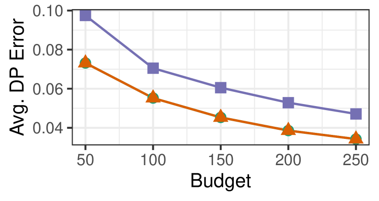
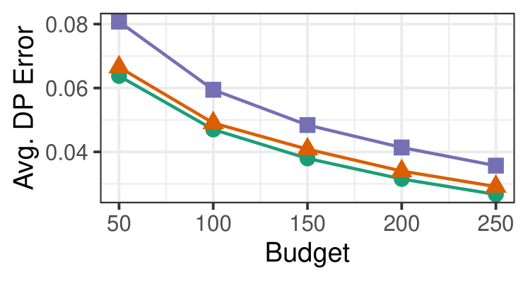
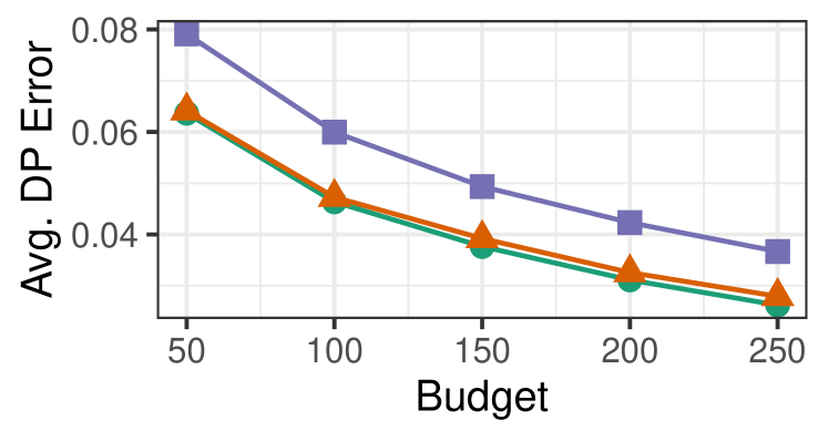
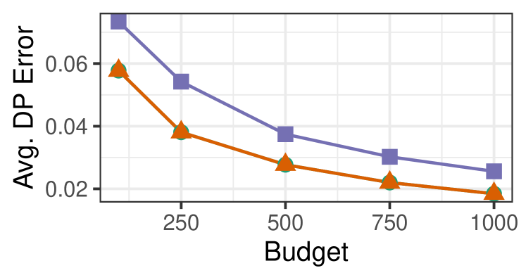
(a) Uniform Sampling

(b) Stratified Sampling

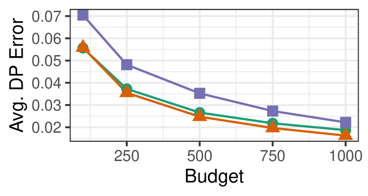
(c) Neyman Sampling

Figure 6: Average error on demographic parity (across agents) for different collaboration and sampling strategies, for the German Credit (top row) and the Propublica dataset (bottom row). Each column corresponds to one sampling method: Uniform (left), Stratified (middle) and Neyman (right).

Appendix D Additional Experiments

This section extends the experimental results presented in Section 6 by presenting the results for the German Credit and Propublica datasets.

D.1 Error of $\hat{D}$ for Two Agents and Increasing Budgets

We simulate the different collaboration and sampling strategies for all three datasets and observe the average error of the DP estimator $\hat{D}$ across agents for different per-agent query budgets $R$, ranging from $50$ to $250$ for German Credit and from $100$ to $1000$ for Propublica. For this experiment, two agents audit a particular attribute in each dataset. We set the attributes to age and gender in the German Credit dataset, African-American origin, and gender in the Propublica dataset. These results are shown in Figure 6 where each row represents a different dataset and each column, a different sampling method. Our first observation is that for all configurations, the average $\hat{D}$ error decreases as $R$ increases since individual $\hat{D}$ estimations become closer to the ground-truth value. Figure 6 also illustrates that a-posteriori or a-priori collaboration always decreases the average $\hat{D}$ error compared to when not collaborating and therefore it is always beneficial to collaborate.

Furthermore, under the same dataset and sampling strategy, the a-posteriori and a-priori collaborations perform similarly. As demonstrated by theory, these two strategies are equivalent when associated uniform sampling. We observe a gap in performance when using stratified or Neyman sampling, without a clear winner. When comparing across sampling methods, we observe that at higher budgets, all strategies achieve similar error values. This is because as the budget rises, the estimations become more accurate independent of the strategy. Consequently, all strategies will converge to the same final error value. At lower budgets, however, the stratified and Neyman sampling methods perform better than uniform sampling. For example, at $R=50$ on the German Credit dataset, a-priori stratified and a-priori Neyman achieve a lower average error ($<0.07$) than a-priori uniform ($>0.07$). Surprisingly, while Neyman sampling is always optimal, stratified sampling performs nearly as well, suggesting that the stratified allocation might not be as far from the Neyman optimal allocation when dealing with only two agents. We extend this comparison between strategies and collaborations further in the Section D.2 while considering more than two agents.

D.2 Error of $\hat{D}$ for Multiple Collaborating Agents

This experiment aims to observe how the average error of $\hat{D}$ changes as we increase the level of collaboration. We use the same setup as described in Section 6.2. We fix the budget value $R=100$ for German Credit and $R=250$ for Propublica. Figure 7 visualizes our results where each row represents a different dataset and each column, a different sampling method.

To begin, we observe that a-posteriori and a-priori are alike with uniform sampling, resulting in overlapping curves in Figure 4 (in line with theory). We observe that, in general, increasing $m$ decreases the average $\hat{D}$ error for collaborative strategies while no collaboration achieves a constant error. Figure 4 shows that for the Neyman sampling, the a-priori strategy always outperforms a-posteriori and no collaboration since it is a theoretically optimal, however, the differences with a-posteriori are minimal. The performance of stratified sampling for collaborative strategies is more nuanced. We observe that, under stratification, the error of a-priori decreases with more collaboration ($m=2$), stabilizes ($m=3,4$) and then even increases at full collaboration ($m=5$) on the Propublica. On the other hand, the error of a-posteriori under stratified sampling always decreases with increasing collaboration. We elucidated further on this relative performance between a-posteriori and a-posteriori strategies under stratified sampling in Section 6.3.

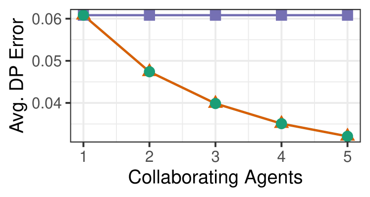
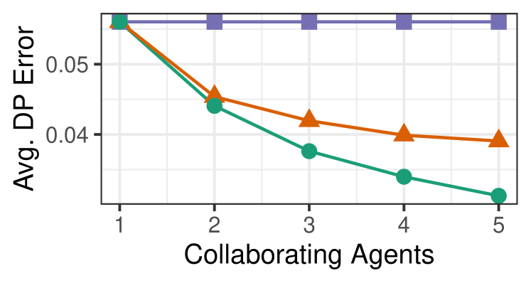
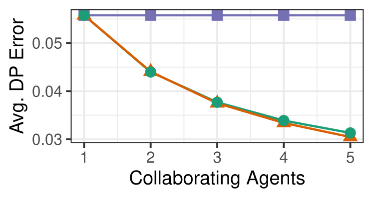
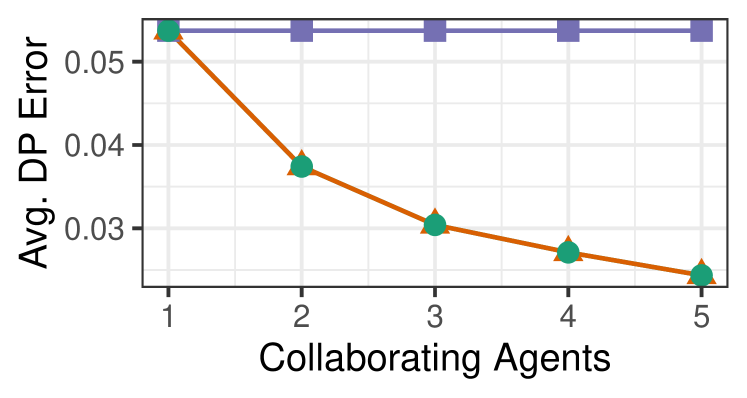
(a) Uniform Sampling

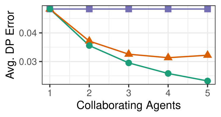
(b) Stratified Sampling

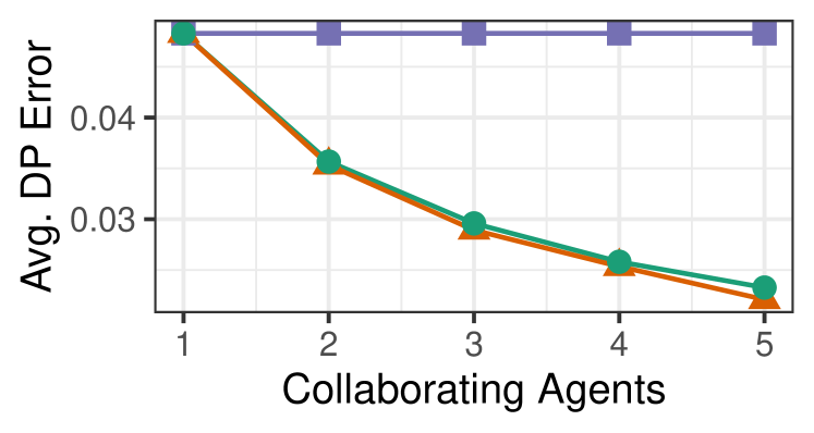
(c) Neyman Sampling

Figure 7: Average error on demographic parity with increasing number of collaborating agents. Each row corresponds to one dataset: German Credit (top row) and Propublica (bottom row). Each column corresponds to one sampling method: Uniform (left), Stratified (middle) and Neyman (right).

Appendix E Discussion

Our analysis results in the following conclusions: • Collaboration is always beneficial (i.e., results in gains $>1$). • The gains of a-priori collaboration are equivalent to or higher than those of a-posteriori collaboration.

References

- Angwin et al. (2016) Angwin, J., Larson, J., Mattu, S., and Kirchner, L. Machine bias: There’s software used across the country to predict future criminals. and it’s biased against blacks. ProPublica, 5 2016.
- Arieska & Herdiani (2018) Arieska, P. K. and Herdiani, N. Margin of error between simple random sampling and stratified sampling. In PROCEEDING International Conference Technopreneur and Education 2018, volume 1, 2018.
- Benjamini & Hochberg (1995) Benjamini, Y. and Hochberg, Y. Controlling the false discovery rate: a practical and powerful approach to multiple testing. Journal of the Royal statistical society: series B (Methodological), 57(1):289–300, 1995.
- Benjamini & Yekutieli (2001) Benjamini, Y. and Yekutieli, D. The control of the false discovery rate in multiple testing under dependency. Annals of statistics, pp. 1165–1188, 2001.
- Buyl & De Bie (2024) Buyl, M. and De Bie, T. Inherent limitations of ai fairness. Communications of the ACM, 2024.
- Cournot (1843) Cournot, A. A. Exposition de la théorie des chances et des probabilités. L. Hachette, 1843.
- Court of justice of the European Union (2023) Court of justice of the European Union. Judgment of the court in case c-252/21, press release no. 113/23, 2023. https://alinea-avocats.eu/fr/actualite/une-autorite-nationale-de-concurrence-est-competente-pour-constater-une-violation-du-rgpd-dans-le-cadre-de-lexamen-dun-abus-de-position-dominante/.
- Crémer et al. (2023) Crémer, J., Dinielli, D., Heidhues, P., Kimmelman, G., Monti, G., Podszun, R., Schnitzer, M., Scott Morton, F., and De Streel, A. Enforcing the digital markets act: institutional choices, compliance, and antitrust. Journal of Antitrust Enforcement, 11(3):315–349, 2023.
- De Jong et al. (2008) De Jong, S., Tuyls, K., and Verbeeck, K. Fairness in multi-agent systems. The Knowledge Engineering Review, 23(2):153–180, 2008.
- Ding et al. (2021) Ding, F., Hardt, M., Miller, J., and Schmidt, L. Retiring adult: New datasets for fair machine learning. Advances in Neural Information Processing Systems, 34, 2021.
- Efron et al. (2001) Efron, B., Tibshirani, R., Storey, J. D., and Tusher, V. Empirical bayes analysis of a microarray experiment. Journal of the American statistical association, 96(456):1151–1160, 2001.
- EU (2022) EU. Auditing the quality of datasets used in algorithmic decision-making systems, 2022. URL https://www.europarl.europa.eu/RegData/etudes/STUD/2022/729541/EPRS_STU(2022)729541_EN.pdf.
- European Commission (2020) European Commission. Proposal for a regulation of the european parliament and of the council on a single market for digital services (digital services act) and amending directive 2000/31/ec., 2020. URL https://digital-strategy.ec.europa.eu/en/library/proposal-regulation-european-parliament-and-council-single-market-digital-services-digital-services.
- European Parliament and Council of the European Union (2022) European Parliament and Council of the European Union. Regulation (eu) 2022/1925 of the european parliament and of the council of 14 september 2022 on contestable and fair markets in the digital sector and amending directives (eu) 2019/1937 and (eu) 2020/1828 (digital markets act), 2022. URL https://eur-lex.europa.eu/eli/reg/2022/1925/oj.
- Fallah et al. (2020) Fallah, A., Mokhtari, A., and Ozdaglar, A. Personalized federated learning with theoretical guarantees: A model-agnostic meta-learning approach. Advances in Neural Information Processing Systems, 33:3557–3568, 2020.
- Feldman et al. (2015) Feldman, M., Friedler, S. A., Moeller, J., Scheidegger, C., and Venkatasubramanian, S. Certifying and removing disparate impact. In proceedings of the 21th ACM SIGKDD international conference on knowledge discovery and data mining, pp. 259–268, 2015.
- Ghezzi et al. (2018) Ghezzi, A., Gabelloni, D., Martini, A., and Natalicchio, A. Crowdsourcing: a review and suggestions for future research. International Journal of management reviews, 20(2):343–363, 2018.
- Giang (2018) Giang, V. The potential hidden bias in automated hiring systems. Fast Company, 2018.
- Gohar & Cheng (2023) Gohar, U. and Cheng, L. A survey on intersectional fairness in machine learning: notions, mitigation, and challenges. In Proceedings of the Thirty-Second International Joint Conference on Artificial Intelligence, IJCAI ’23, 2023. ISBN 978-1-956792-03-4. doi: 10.24963/ijcai.2023/742. URL https://doi.org/10.24963/ijcai.2023/742.
- Hofmann (1994) Hofmann, H. Statlog (German Credit Data). UCI Machine Learning Repository, 1994. DOI: https://doi.org/10.24432/C5NC77.
- Holstein et al. (2019) Holstein, K., Wortman Vaughan, J., Daumé III, H., Dudik, M., and Wallach, H. Improving fairness in machine learning systems: What do industry practitioners need? In Proceedings of the 2019 CHI conference on human factors in computing systems, pp. 1–16, 2019.
- Hunkenschroer & Luetge (2022) Hunkenschroer, A. L. and Luetge, C. Ethics of ai-enabled recruiting and selection: A review and research agenda. Journal of Business Ethics, 178(4):977–1007, 2022.
- Keramat & Kielbasa (1998) Keramat, M. and Kielbasa, R. A study of stratified sampling in variance reduction techniques for parametric yield estimation. IEEE Transactions on Circuits and Systems II: Analog and Digital Signal Processing, 45(5):575–583, 1998.
- Kloek & Van Dijk (1978) Kloek, T. and Van Dijk, H. K. Bayesian estimates of equation system parameters: an application of integration by monte carlo. Econometrica: Journal of the Econometric Society, pp. 1–19, 1978.
- Le Merrer et al. (2023) Le Merrer, E., Pons, R., and Trédan, G. Algorithmic audits of algorithms, and the law. AI and Ethics, pp. 1–11, 2023.
- Mathew et al. (2013) Mathew, O. O., Sola, A. F., Oladiran, B. H., and Amos, A. A. Efficiency of neyman allocation procedure over other allocation procedures in stratified random sampling. American Journal of Theoretical and Applied Statistics, 2(5):122–127, 2013.
- Mhlanga (2021) Mhlanga, D. Financial inclusion in emerging economies: The application of machine learning and artificial intelligence in credit risk assessment. International journal of financial studies, 9(3):39, 2021.
- Mikians et al. (2013) Mikians, J., Gyarmati, L., Erramilli, V., and Laoutaris, N. Crowd-assisted search for price discrimination in e-commerce: First results. In Proceedings of the ninth ACM conference on Emerging networking experiments and technologies, pp. 1–6, 2013.
- Mouzannar et al. (2019) Mouzannar, H., Ohannessian, M. I., and Srebro, N. From fair decision making to social equality. In Proceedings of the Conference on Fairness, Accountability, and Transparency, pp. 359–368, 2019.
- Neiswanger et al. (2021) Neiswanger, W., Wang, K. A., and Ermon, S. Bayesian algorithm execution: Estimating computable properties of black-box functions using mutual information. In International Conference on Machine Learning, pp. 8005–8015. PMLR, 2021.
- Ng (2021) Ng, A. Can auditing eliminate bias from algorithms?, Feb 2021. URL https://themarkup.org/the-breakdown/2021/02/23/can-auditing-eliminate-bias-from-algorithms. Accessed: 2023-10-10.
- Pessach & Shmueli (2022) Pessach, D. and Shmueli, E. A review on fairness in machine learning. ACM Computing Surveys (CSUR), 55(3):1–44, 2022.
- Rastegarpanah et al. (2021) Rastegarpanah, B., Gummadi, K., and Crovella, M. Auditing black-box prediction models for data minimization compliance. Advances in Neural Information Processing Systems, 34:20621–20632, 2021.
- Saleiro et al. (2018) Saleiro, P., Kuester, B., Hinkson, L., London, J., Stevens, A., Anisfeld, A., Rodolfa, K. T., and Ghani, R. Aequitas: A bias and fairness audit toolkit. arXiv preprint arXiv:1811.05577, 2018.
- Shaffer (1995) Shaffer, J. P. Multiple hypothesis testing. Annual review of psychology, 46(1):561–584, 1995.
- Shen et al. (2020) Shen, T., Zhang, J., Jia, X., Zhang, F., Huang, G., Zhou, P., Kuang, K., Wu, F., and Wu, C. Federated mutual learning. arXiv preprint arXiv:2006.16765, 2020.
- Singh & Chunara (2023) Singh, H. and Chunara, R. Measures of disparity and their efficient estimation. In Proceedings of the 2023 AAAI/ACM Conference on AI, Ethics, and Society, pp. 927–938, 2023.
- Smith et al. (2017) Smith, V., Chiang, C.-K., Sanjabi, M., and Talwalkar, A. S. Federated multi-task learning. Advances in neural information processing systems, 30, 2017.
- Xu et al. (2023) Xu, X., Wu, Z., Verma, A., Foo, C. S., and Low, B. K. H. Fair: Fair collaborative active learning with individual rationality for scientific discovery. In Ruiz, F., Dy, J., and van de Meent, J.-W. (eds.), Proceedings of The 26th International Conference on Artificial Intelligence and Statistics, volume 206 of Proceedings of Machine Learning Research, pp. 4033–4057. PMLR, 25–27 Apr 2023. URL https://proceedings.mlr.press/v206/xu23e.html.
- Yan & Zhang (2022) Yan, T. and Zhang, C. Active fairness auditing. In International Conference on Machine Learning, pp. 24929–24962. PMLR, 2022.
- Zhang et al. (2021) Zhang, C., Xie, Y., Bai, H., Yu, B., Li, W., and Gao, Y. A survey on federated learning. Knowledge-Based Systems, 216:106775, 2021.
- Zhang & Yang (2021) Zhang, Y. and Yang, Q. A survey on multi-task learning. IEEE Transactions on Knowledge and Data Engineering, 34(12):5586–5609, 2021.