Counterfactual Influence in Markov Decision Processes

Abstract

Our work addresses a fundamental problem in the context of counterfactual inference for Markov Decision Processes (MDPs). Given an MDP path $\tau$, this kind of inference allows us to derive counterfactual paths $\tau^{\prime}$ describing what-if versions of $\tau$ obtained under different action sequences than those observed in $\tau$. However, as the counterfactual states and actions deviate from the observed ones over time, the observation $\tau$ may no longer influence the counterfactual world, meaning that the analysis is no longer tailored to the individual observation, resulting in interventional outcomes rather than counterfactual ones. Even though this issue specifically affects the popular Gumbel-max structural causal model used for MDP counterfactuals, it has remained overlooked until now. In this work, we introduce a formal characterisation of influence based on comparing counterfactual and interventional distributions. We devise an algorithm to construct counterfactual models that automatically satisfy influence constraints. Leveraging such models, we derive counterfactual policies that are not just optimal for a given reward structure but also remain tailored to the observed path. Even though there is an unavoidable trade-off between policy optimality and strength of influence constraints, our experiments demonstrate that it is possible to derive (near-)optimal policies while remaining under the influence of the observation.

1 Introduction

Counterfactual inference allows us to reason hypothetically about what effect changing an action or condition in the past would have on a given observation, e.g., “What would the patient’s condition be, had we used treatment Y instead of treatment X?”. This type of reasoning is particularly useful for evaluating and optimising sequences of actions, to identify how the end result could have been improved by changing some action(s) along the observed path. This optimised counterfactual path can be seen as a counterfactual explanation of how the decision-making process could be improved. Markov Decision Processes (MDPs) are often used to model sequential decision-making processes under uncertainty, so counterfactual inference can be used to generate counterfactual explanations on improving a given policy. This research area also aligns with the increasing use of machine learning in healthcare, specifically in supporting clinical decision-making with the use of AI models (Verma et al., 2020; Guidotti, 2022; Tsirtsis et al., 2021).

One of the key issues in sequential processes, which is not as pronounced in single-step scenarios, is the divergence of the counterfactual path from the observed one: as the counterfactual outcomes deviate over time, the observations become less relevant for counterfactual inference. In particular, this problem involves categorical counterfactual models used for MDPs. This leads to a situation where we are essentially computing interventional outcomes rather than counterfactual ones, meaning that the outcomes are no longer tailored to the specific observed path.

Consider an example of clinical decision-making where we observe a patient transitioning from state $s$ into state $s^{\prime}$ after a therapy action $a$. Formally, $s^{\prime}$ arises from some structural causal model (SCM), $s^{\prime}\sim f(s,a,\mathbf{U})$, where $\mathbf{U}$ are the (prior) random exogenous factors and $f$ is a function. Now, suppose that the observed $s^{\prime}$ is a particularly unlikely next state given $s$ and $a$ (e.g., the patient’s sugar levels increase after administering insulin, or oxygen levels drop after giving an anticoagulant). Thus, we may be interested in the following counterfactual query: what would have been the patient’s next state at state $s_{c}$ if we delivered a different therapy decision $a_{c}\neq a$, given that we observed the path $\tau=(s,a,s^{\prime})$? In counterfactual inference, this amounts to deriving the posterior $\mathbf{U}^{\prime}=\mathbf{U}\mid\tau$ and then predicting $S^{\prime}_{c}\sim f(s_{c},a_{c},\mathbf{U}^{\prime})$. In this example, given that observing $s^{\prime}$ was a rare event, the posterior $\mathbf{U}^{\prime}$ makes $s^{\prime}$ much more likely, penalising other states that could have been reached from $s$ and $a$. However, it does not influence the likelihood of states that are impossible from $s$ and $a$ (not observing them does not bring any new information). Similarly, if $s^{\prime}$ is impossible from $s_{c}$ and $a_{c}$, then it remains so in the counterfactual world too, no matter how strong the evidence provided by $\mathbf{U}^{\prime}$ in favour of $s^{\prime}$. Hence, there may be cases when the counterfactual state $s_{c}$ diverges from the observed $s$ (which is the norm in sequential processes) in such a way that the distribution of our counterfactual outcome $S^{\prime}_{c}$ is not at all influenced by the observation $\tau$. We illustrate the notion of influence in Figure 1, with an artificial example of insulin therapy in type 1 diabetes.

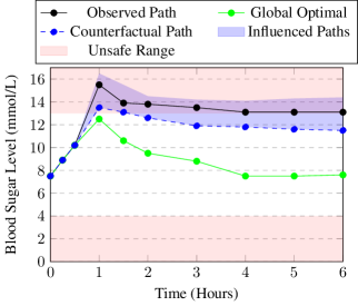
Figure 1: Given an observed path (black), we can reason counterfactually about adjusting bolus insulin to carbohydrate ratios for type 1 diabetes patients. Shaded in blue is the range of possible counterfactual paths that are influenced by the observed path, from which we identify the optimal one (blue). Without influence constraints, we may find better outcomes (green), but these would be disconnected from the individual observation (i.e., such outcomes are interventional, not counterfactual).

We build on recent work by Oberst & Sontag (2019) who introduced Gumbel-max SCMs, a class of causal models for counterfactual inference of discrete-state MDPs, as well as on the approach of Tsirtsis et al. (2021), which leverages Gumbel-max SCMs to derive an alternative sequence of actions that optimises the counterfactual outcome but do not differ much from the observed sequence. However, these and other existing papers on counterfactual analysis of MDPs, e.g. (Buesing et al., 2018; Lu et al., 2020; Kazemi & Paoletti, 2023), ignore the issue of influence, resulting in counterfactuals that may be (erroneously) disconnected from the observation.

Contributions. In this paper, we introduce the notion of influence in the context of counterfactual inference of MDPs. In particular, we say that an MDP path influences the counterfactual world if the interventional probabilities (i.e., the transition probabilities of the nominal MDP under the counterfactual policy) and the corresponding counterfactual probabilities are not identical. In this way, our approach can devise counterfactual policies that are not only optimal for a given reward structure but also maintain a degree of influence from the observed path, meaning that the counterfactual outcome remains tailored to the individual observation.

Procedurally, we build a counterfactual MDP that inherently satisfies influence constraints, through a polynomial-time algorithm that prunes the (non-constrained) counterfactual MDP removing all actions that lead in one step into states that violate influence. Hence, our approach has also the benefit of reducing the MDP’s size. We note that imposing such constraints over one step only may result in counterfactual MDPs that are close or equal to the observed path, which is not desirable when the path describes an unsafe evolution (e.g., a patient progresses to an unrecoverable condition). Therefore, we further extend the notion of influence to encompass multiple steps, so that influence constraints must hold at least once (as opposed to always) over paths of a given length. In this way, we can arbitrarily relax influence constraints, allowing for larger deviations from the observation, to favour optimality of the counterfactual policy.

We validate our approach on a grid-world model and two clinical case studies: an epidemic model and a sepsis model. We evaluate how relaxing influence constraints impact the optimal policy derived for a counterfactual MDP. In particular, we find that our approach results in counterfactual paths that are optimal or near-optimal while remaining influenced by the observed path. This results in more informative counterfactual explanations for improving a given policy, as these explanations are guaranteed to be tailored toward the given observation.

2 Preliminaries

MDPs are a class of stochastic models to describe sequential decision-making processes. In an MDP $\mathcal{P}$, at each step $t$, an agent in state $s_{t}$ performs some action $a_{t}$ determined by a policy $\pi$, ending up in state $s_{t+1}\sim P_{\mathcal{P}}(s\mid s_{t},a_{t})$. The agent receives some reward $R(s_{t},a_{t})$ for performing $a_{t}$ at $s_{t}$. Formally, an MDP is a tuple $\mathcal{P}=(\mathcal{S},\mathcal{A},P_{\mathcal{P}},P_{I},R)$ where $\mathcal{S}$ is the discrete state space, $\mathcal{A}$ is the set of actions, $P_{\mathcal{P}}:(\mathcal{S}\times\mathcal{A}\times\mathcal{S})\rightarrow[0,1]$ is the transition probability function, $P_{I}:\mathcal{S}\rightarrow[0,1]$ is the initial state distribution, and $R:(\mathcal{S}\times\mathcal{A})\rightarrow\mathbb{R}$ is the reward function. A (deterministic) policy $\pi$ for $\mathcal{P}$ is a function $\pi:\mathcal{S}\rightarrow\mathcal{A}$. A path realisation of $\mathcal{P}$ under policy $\pi$, denoted $\tau\sim\mathcal{P}(\pi)$, is a sequence $\tau=(s_{0},a_{0}),(s_{1},a_{1}),\ldots,(s_{T-1},a_{T-1})$ where $T=|\tau|$ is the path length, $P_{I}(s_{0})>0$, $a_{t}=\pi(s_{t})$ for all $t=0,\ldots,T-1$, and $P_{\mathcal{P}}(s_{t+1}\mid s_{t},a_{t})>0$ for all $t=0,\ldots,T-2$.

While the MDP characterisation helps make predictions about future states and design action policies, it is not sufficient to make counterfactual predictions. For this purpose, we need Structural Causal Models (SCMs) (Pearl, 2009). Formally, an SCM is a tuple $\mathcal{M}=(\mathbf{U},\mathbf{V},\mathcal{F}=\{f_{V}\}_{V\in\mathbf{V}},P(\mathbf{U}))$, where $\mathbf{U}$ is a set of mutually independent exogenous variables with $P(\mathbf{U})$ being its distribution, and $\mathbf{V}$ is a set of endogenous variables. The value of each $V\in\mathbf{V}$ is determined by a function $V=f_{V}(\mathbf{PA}_{V},U_{V})$ where $\mathbf{PA}_{V}\subseteq\mathbf{V}$ is the set of direct causes of $V$ and $U_{V}\in\mathbf{U}$. Assignments in an SCM are acyclic, so that no variable can be a direct or indirect cause of itself.

Endogenous variables are those that can be observed. Exogenous variables are unobserved and act as the source of randomness in the model. Indeed, for a fixed realisation $\mathbf{u}\sim P(\mathbf{U})$, i.e., a concrete unfolding of the system’s randomness, the values of $\mathbf{V}$ become deterministic, as they are uniquely determined by $\mathbf{u}$ and $\mathcal{F}$. The value $\mathbf{u}$ is called context. With SCMs, one can establish the causal effect of some input variable $X$ on some outcome $Y$ by evaluating $Y$ after applying a so-called intervention $X\leftarrow x$, i.e., after replacing the RHS of $X=f_{X}(\mathbf{PA}_{X},U_{X})$ with $x$. We denote the resulting interventional distribution by $P_{\mathcal{M}[x]}(Y)$ (also written as $P(Y\mid\mathit{do}(x))$ in Pearl’s do notation).

Upon observing a realisation $\mathbf{v}$ of the SCM variables $\mathbf{V}$, counterfactuals answer the following question: what would have been the value of variable $Y$ under intervention $X\leftarrow x$, given that we observed $\mathbf{v}$? This corresponds to evaluating $\mathbf{V}$ in a hypothetical world characterised by the same context that generated the observation $\mathbf{v}$ but under a different causal process (i.e., $\mathcal{M}[x]$ instead of $\mathcal{M}$). Computing counterfactuals first requires deriving the context that led to the observation, i.e., $\mathbf{U}\mid\mathbf{v}$, and then evaluate the outcome under the counterfactual model obtained from $\mathcal{M}[x]$ by replacing $P(\mathbf{U})$ with the inferred $P(\mathbf{U}\mid\mathbf{v})$. Since each observation $\mathbf{v}$ can be seen as a deterministic function of a particular context $\mathbf{u}$, then in theory, the counterfactual outcome should be deterministic too. However, as we will see, $\mathbf{u}$ cannot be always uniquely identified from $\mathbf{v}$, resulting in a (non-Dirac) posterior distribution $P(\mathbf{U}\mid\mathbf{v})$ and a stochastic counterfactual outcome.

2.1 SCM-based Encoding of MDPs

To enable counterfactual reasoning in MDPs, Oberst & Sontag (2019) have proposed the following SCM-based encoding. For an MDP $\mathcal{P}$, policy $\pi$, and horizon $T$, we define an SCM over variables $\{S_{t},A_{t}\}_{t=0}^{T-1}$ which describes paths of length $T$ induced by $\mathcal{P}$ and $\pi$, using the structural equations:

$$S_{t+1}=f(S_{t},A_{t},U_{t});\ \ A_{t}=\pi(S_{t});\ \ S_{0}=f_{0}(U_{0}).$$ (1)

In the above equations, we factorise the model into an independent source of noise (the exogenous variables $U_{t}$) and a deterministic function mapping such noise variables into values of the endogenous variables (i.e., the MDP states and actions). This factorisation allows us to compute counterfactuals, but it is not obvious how to define $f$ (and $f_{0}$) when dealing with categorical variables (arising from the MDP’s discrete state space). To this purpose, Oberst & Sontag (2019) introduced Gumbel-Max SCMs, expressed as

$$\begin{array}[]{ll}S_{t+1}&=f(S_{t},A_{t},U_{t}=(G_{s,t})_{s\in\mathcal{S}})\\ &=\operatorname*{arg\,max}_{s\in\mathcal{S}}\left\{\log\left(P_{\mathcal{P}}(s\mid S_{t},A_{t})\right)+G_{s,t}\right\},\end{array}$$ (2)

where for each $s\in\mathcal{S}$ and $t=0,\ldots,T-1$, $G_{s,t}$ follows a Gumbel distribution. This approach is grounded in the Gumbel-Max trick, which shows that sampling from a categorical distribution with $k$ categories is equivalent to sampling $k$ copies $g_{0},\ldots,g_{k}$ of a standard Gumbel and then determining the outcome as $\operatorname*{arg\,max}_{j}\left\{\log\left(P(Y=j)\right)+g_{j}\right\}$. Notably, the Gumbel-Max SCM encoding possesses a desirable feature called counterfactual stability, which, informally, states that a counterfactual outcome remains equal to the observed outcome unless the intervention increases the relative probability of an alternative outcome. See (Oberst & Sontag, 2019) for more details.

Counterfactual inference.

Given an MDP path $\tau=(s_{0},a_{0}),\ldots,(s_{T-1},a_{T-1})$, the task of counterfactual inference in this context is to identify the values of the Gumbel exogenenous variables that align with $\tau$, i.e., calculate $\mathbf{G}^{\prime}=(G_{s,t})_{s\in\mathcal{S}}^{t=0,\ldots,T-1}\mid\tau$. Thanks to the Markov property, their probability can be decomposed as:

$$P(\mathbf{G}^{\prime})=P((G_{s,0})_{s\in\mathcal{S}}\mid s_{1})\cdot\prod_{t=1}^{T-1}P((G_{s,t})_{s\in\mathcal{S}}\mid s_{t},a_{t},s_{t+1}).$$ (3)

Yet, a challenge arises as the mechanism of (2) is non-invertible: for given $s_{t}$ and $a_{t}$, multiple sets of $(G_{s,t})_{s\in\mathcal{S}}$ can result in the same $s_{t+1}$. This implies that MDP counterfactuals cannot be uniquely identified, an issue that affects not just Gumbel-Max SCMs but categorical counterfactuals in general (Oberst & Sontag, 2019). As proposed by Oberst & Sontag, (approximate) posterior inference of $P((G_{s,t})_{s\in\mathcal{S}}\mid s_{t},a_{t},s_{t+1})$ can be nevertheless accomplished through rejection sampling: we first draw samples from the prior $(g_{s,t})_{s\in\mathcal{S}}\sim P((G_{s,t})_{s\in\mathcal{S}})$ and then discard all instances where $f(s_{t},a_{t},(g_{s,t})_{s\in\mathcal{S}})\neq s_{t+1}$. This can also be implemented more efficiently using the top-down Gumbel sampling approach described in (Maddison et al., 2014).

2.2 Counterfactual MDP and Optimal Policies

Once derived the posterior Gumbel variables $\mathbf{G}^{\prime}$ as described above, we can define a corresponding counterfactual MDP $\mathcal{P}^{\tau}$, which captures counterfactual probabilities at any choice of state $s$ and action $a$. $\mathcal{P}^{\tau}$ is a non-stationary MDP with the same state space $\mathcal{S}$, action space $\mathcal{A}$, and reward structure $R$ as $\mathcal{P}$; its initial state distribution $P^{\tau}_{I}$ assigns probability $1$ to $s_{0}$, the first state of $\tau$; and its transition probability function directly follows from the SCM (2) and is defined, for $t=0,\ldots,T-1$, as

$$P_{\mathcal{P},t,\tau}(s^{\prime}\mid s,a)=\\ \underset{(G^{\prime}_{s^{\prime\prime},t})_{s^{\prime\prime}\in\mathcal{S}}}{\mathrm{Pr}}\left(s^{\prime}=\operatorname*{arg\,max}_{s^{\prime\prime}\in\mathcal{S}}\left\{\log\left(P_{\mathcal{P}}(s^{\prime\prime}\mid s,a)\right)+G^{\prime}_{s^{\prime\prime},t}\right\}\right).$$ (4)

Such MDP can be directly solved to derive optimal counterfactual policies, as done in (Tsirtsis et al., 2021). The authors, in particular, are concerned with finding optimal action sequences that differ in at most $m$ actions from the observed sequence. We call this an $m$-CF policy.

Definition 2.1 ($m$-CF policy (Tsirtsis et al., 2021)).

Let $\tau$ be a path of an MDP $\mathcal{P}$ of length $T$, and let $\mathcal{P}^{\tau}$ be the corresponding counterfactual MDP. For a given $m\leq T$, an $m$-CF policy $\pi^{*}$ is one that maximises the value $V_{\tau}(\pi)=\mathbb{E}_{\tau^{\prime}\sim\mathcal{P}^{\tau}(\pi)}\left[\sum_{t=0}^{T-1}R(s^{\prime}_{t},a^{\prime}_{t})\right]$ under the condition that any counterfactual path $\tau^{\prime}$ induced by $\mathcal{P}^{\tau}$ and $\pi^{*}$ satisfies $\sum_{t=0}^{T-1}\mathbf{1}(a_{t}\neq a^{\prime}_{t})\leq m$.

To derive $m$-CF policies, Tsirtsis et al. employ a polynomial-time dynamic programming algorithm that keeps track of the number of action changes between the observed path $\tau$ and the counterfactual one $\tau^{\prime}$. However, their approach has two main shortcomings. First, $\tau^{\prime}$ may diverge from $\tau$, visiting different state sequences where it may not be sensible to impose the same observed action. Second, and most important, because of this divergence, it is possible to reach a state in $\tau^{\prime}$ where the observed path $\tau$ bears no longer influence, meaning that we are no longer computing counterfactuals but interventional outcomes. In the next sections, we formally characterise and solve the latter issue.

3 Theoretical Framework

In this section, we introduce the notion of influence in the context of MDP counterfactuals, to characterise the degree to which an observed path $\tau$ affects the counterfactual world. As stated previously, when there is no influence, then the counterfactual distribution $P_{\mathcal{P},t,\tau}$ is identical to the original/interventional one $P_{\mathcal{P}}$. Before formally defining influence, below we derive a sufficient condition for these two distributions to be equal.

Proposition 3.1.

Let $\tau$ be a path of an MDP $\mathcal{P}$ of length $T$, and let $\mathcal{P}^{\tau}$ be the corresponding counterfactual MDP. Given a time $t<T$ and counterfactual state $s^{\prime}_{t}$ and action $a^{\prime}_{t}$ in $\mathcal{P}^{\tau}$, then if $P_{\mathcal{P}}(\cdot\mid s_{t},a_{t})$ and $P_{\mathcal{P}}(\cdot\mid s^{\prime}_{t},a^{\prime}_{t})$ have disjoint support, then the counterfactual distribution $P_{\mathcal{P},t,\tau}(\cdot\mid s^{\prime}_{t},a^{\prime}_{t})$ is identical to the interventional distribution $P_{\mathcal{P}}(\cdot\mid s^{\prime}_{t},a^{\prime}_{t})$.

Proof.

At time $t$, if the distributions $P_{\mathcal{P}}(\cdot\mid s_{t},a_{t})$ and $P_{\mathcal{P}}(\cdot\mid s^{\prime}_{t},a^{\prime}_{t})$ have disjoint supports then the posterior Gumbel distribution relative to the possible next states from $(s^{\prime}_{t},a^{\prime}_{t})$ remains the same as the prior Gumbel distribution for those states. This is because the states in the support of $P(\cdot\mid s^{\prime}_{t},a^{\prime}_{t})$ cannot be reached from $(s_{t},a_{t})$ in the factual world (i.e., in the original MDP), hence, no observation can change their prior. As a consequence, by (2) and (4), the counterfactual probabilities for those states remain equal to the probabilities in the original MDP. ∎

With this proposition, we can now define influence by checking a simple condition on the transition probabilities of the original MDP. Importantly, this condition can be checked precisely because we know the true probabilities $P_{\mathcal{P}}$. On the other hand, the equality $P_{\mathcal{P},t,\tau}(\cdot\mid s^{\prime}_{t},a^{\prime}_{t})=P_{\mathcal{P}}(\cdot\mid s^{\prime}_{t},a^{\prime}_{t})$ cannot be established precisely because of the sampling error introduced in $P_{\mathcal{P},t,\tau}$ by the Gumbel posterior inference.

Definition 3.2 (1-step influence).

Let $\tau$ be a path of an MDP $\mathcal{P}$ of length $T$, and let $\mathcal{P}^{\tau}$ be the corresponding counterfactual MDP. Given a time $t<T$ and counterfactual state $s^{\prime}_{t}$ and action $a^{\prime}_{t}$ in $\mathcal{P}^{\tau}$, we say that $\tau$ exerts an immediate ($1$- step) influence on $s^{\prime}_{t}$ and $a^{\prime}_{t}$ at time $t$ if and only if the supports of the distributions $P_{\mathcal{P}}(\cdot\mid s^{\prime}_{t},a^{\prime}_{t})$ and $P_{\mathcal{P}}(\cdot\mid s_{t},a_{t})$ are not disjoint.

While imposing influence constraints is clearly desirable, the above notion of $1$-step influence may be too strict and we may not be able to deviate much, or at all, from the observed path. Figure 2b provides an example of a toy counterfactual MDP, with two possible actions: $a_{0}$ (which has a distribution of possible outcomes) and $a_{1}$ (which is deterministic). With a 1-step influence, although there are three state-action pairs (in addition to those in the observed path) that are influenced by the observed path, states $s_{4}$ and $s_{6}$ are not reachable, and so the only possible counterfactual paths are the observed path and the path through state $s_{3}$.

(a)

(b) $k=1$

(c) $k=2$

Figure 2: Example counterfactual MDP given $k$-step influence

To overcome this potential limitation, we relax and generalise the notion of $1$-step influence to encompass multiple steps, so that influence constraints needs to hold at least once in a counterfactual path, and not at every step.

Definition 3.3 ($k$-step influence).

Let $\mathcal{P}$, $T$, $\tau$, and $\mathcal{P}^{\tau}$ be as in Definition 3.2. Given a time $t<T$, horizon $k$, and counterfactual state $s^{\prime}_{t}$ and action $a^{\prime}_{t}$, if $t+k<T$ we say that $\tau$ exerts a $k$-step influence on $s^{\prime}_{t}$ and $a^{\prime}_{t}$ at time $t$ if there exists a path $\tau^{\prime}$ of $\mathcal{P}^{\tau}$ of length $k$ starting in $(s^{\prime}_{t},a^{\prime}_{t})$ and such that $\tau$ exerts a $1$-step influence on at least one state of $\tau^{\prime}$. If $t+k\geq T$, $\tau$ always exerts a $k$-step influence on $s^{\prime}_{t}$ and $a^{\prime}_{t}$ at time $t$.

Remark 3.4.

In the above definition, when $t+k\geq T$, the length $T$ of the observed path is not sufficient to determine $k$-step influence, and so we make the conservative assumption that influence holds in such cases. In particular, for $k\geq T$, we have that the observed path $\tau$ exerts a $k$-step influence on any counterfactual state at any time $t$ (because when $k\geq T$, then $t+k\geq T$ for any $t$).

Figure 2c extends Figure 2b to consider 2-step influence. This further expands the set of paths that can be taken in the counterfactual MDP, which may lead to better outcomes. For this example, a $k$-step influence of $k\geq 3$ suffices to recover all transitions from the original MDP.

We now re-formulate the idea of optimal counterfactual policy by incorporating our notion of influence. Previously, in Definition 2.1, we restricted to policies ensuring a bounded number of action changes from the observed action sequence. Here, we further include constraints to guarantee that any counterfactual path is influenced to some degree by the observation.

Definition 3.5 ($(k,m)$-CF policy).

Let $\tau$ be a path of an MDP $\mathcal{P}$ of length $T$, and let $\mathcal{P}^{\tau}$ be the corresponding counterfactual MDP. For a given $m\leq T-1$ and influence bound $k$, a $(k,m)$-CF policy $\pi^{*}$ is one that maximises the value $V_{\tau}(\pi)=\mathbb{E}_{\tau^{\prime}\sim\mathcal{P}^{\tau}(\pi)}\left[\sum_{t=0}^{T-1}R(s^{\prime}_{t},a^{\prime}_{t})\right]$ under two conditions: 1) the observed path $\tau$ exerts a $k$-step influence on any counterfactual path $\tau^{\prime}$ induced by $\mathcal{P}^{\tau}$ and $\pi^{*}$; and 2) any such counterfactual path satisfies the constraint $\sum_{t=0}^{T-1}\mathbf{1}(a_{t}\neq a^{\prime}_{t})\leq m$.

4 Methodology

In this section, we describe the implementation for finding the optimal $(k,m)$-CF policy for a given MDP. To do this, we must first restrict the counterfactual MDP to only transitions that are influenced by the observed path (under a $k$-step influence).

We implement this by first identifying, for each state-action $(s_{t},a_{t})$ pairs in the observed path, all states $s$ that are in the support of $P(\cdot\mid s_{t},a_{t})$. We denote the set of such states with $S^{\tau}_{t}$, and denote the union of all of these $S^{\tau}_{t}$ as $S^{\tau}=\bigcup_{t=0}^{T-1}S^{\tau}_{t}$. For the example MDP given in Figures 2b and 2c, $S^{\tau}=\{s_{2},s_{3},s_{5},s_{8}\}$.

We then execute a reverse Breadth-First Search (BFS) algorithm with a maximum depth of $k$ over the original MDP, starting from each state in $S^{\tau}$. This identifies all the states that can reach a transition influenced by the observed path, within $k$ steps, which we denote as $S^{\tau,k}$. As shown in Figure 2b, $S^{\tau,1}=S^{\tau}\cup\{s_{4},s_{6}\}$, and $S^{\tau,2}=S^{\tau}\cup\{s_{1},s_{4},s_{6}\}$. We remark that, since the BFS algorithm is polynomial in the number of states and transitions, and we run the algorithm $|S^{\tau}|$ times, the computational complexity of the algorithm remains polynomial.

Next, we build the influence-constrained counterfactual MDP by adding all transitions (with their counterfactual probabilities $P_{\mathcal{P},t,\tau}$) between the states in $S^{\tau,k}$. As stated in Definition 3.3, we also need to include all transitions between $t=T-k+1$ and $t=T$, since the observed path always exerts a $k$-step influence over any path of length $<k$ in this range. Finally, we need to remove any states that are unreachable or have no outgoing transitions, and all actions that have some probability of leading to states outside the pruned counterfactual MDP. This is necessary to ensure that we never reach states outside the pruned counterfactual MDP. As shown in Figures 2b and 2c, this last pruning step removes states $s_{4}$ and $s_{6}$ for $k=1$, and states $s_{1}$ and $s_{4}$ for $k=2$, as these states are not reachable. Pseudocode for the algorithm can be found in Appendix A.

Once the influence-constrained counterfactual MDP is constructed, we use a similar dynamic programming approach to value iteration as described in (Tsirtsis et al., 2021) to find the optimal $(k,m)$-CF policy for each given $m$ (the maximum number of actions that can be changed). The only difference is that we restrict the action choices to only those transitions in the influence-constrained MDP.

5 Experiments

In this section, we apply our notion of influence to several MDPs, to derive counterfactual policies with a varying level of influence with respect to the observed path. We evaluate our approach on three models: a Grid World example, an epidemic MDP model, and a realistic MDP for modelling the progression of a patient with sepsis.

5.1 Setup

For each MDP, we first generate an observed path of length $T$ using a deliberately sub-optimal policy. The exact value of $T$ depends on the MDP being evaluated, to ensure there is enough opportunity to improve the policy, and is noted in the following subsections. We use this observed path to generate the optimal $(k,m)$-CF policy for $1\leq k\leq T+1$ and $1\leq m\leq T$, using the algorithm described in Section 4. We always assume that counterfactual paths begin in the same initial state as the observed path. To evaluate the performance of the $(k,m)$-CF policies, we consider the value of the initial state, $V(s_{0})$, as this measures how good the paths generated by the optimal policy (starting at the initial state) will be.

Our algorithm was implemented in Python 3.10 and executed on an 128 core machine with NVIDIA A40 48GB GPU, Intel Xeon CPU and 512 GB RAM.

5.2 Grid World

In the Grid World experiment, the agent must traverse a 4x4 grid from the top-left corner to the bottom-right corner, avoiding a dangerous terminal state in the middle of the grid. At each time step, the agent can move up, down, left, or right. However, there is a small probability that the agent will move in a different direction to the chosen action. As the agent gets closer to the goal state in the bottom-right corner, the reward for each state increases, and the agent receives a reward of $100$ for reaching the terminal goal state. However, there is also a reward of $-100$ for transitioning into the dangerous terminal state.

We derive the counterfactual MDP using an observed path of length 11 that falls into this dangerous terminal state at time 3. Figure 3 shows how $k$ and $m$ affect the value collected by the $(k,m)$-CF policy. For a $k$-step influence of $k\leq 6$, we see no improvement in the optimal policy, since all influenced paths of 6 steps or fewer lead back to the dangerous terminal state. However, the goal state can be reached with a $k$-step influence of $k\geq 7$, which gives the maximum possible value for the initial state. In this case, we can generate counterfactual paths which are still influenced by the observed path, and so are more informed than those paths for $k=T+1$.

Figure 3: Grid World: value of initial state given $k$-step influence and maximum $m$ actions changed

5.3 Epidemic Model

In this experiment, the MDP describes how infection spreads through a (discrete) population. Each state $(S,I,V)$ consists of $S$ susceptible and $I$ infected individuals, and the number of available vaccines $V$. At each time step, the agent implements a vaccination strategy and can choose among three actions: do nothing, vaccinate an infected individual, or vaccinate a susceptible individual. We use a hypergeometric distribution to model how many susceptible individuals become infected at each step. Each vaccination decreases the count $V$ and removes the vaccinated individual from the population (i.e., no re-infection is possible). The reward for each transition $(s,a,s^{\prime})$ is given by the negative of the number of infected individuals in $s$, $-I$. Full details of the model are given in Appendix B.

The observed path of length 7 begins in state $(S=9,I=1,V=20)$ and is generated from a suboptimal policy that does nothing in every state. We can therefore generate increasingly better counterfactual paths that are still highly influenced by the observed path, because switching the action in most states would lead to an improved outcome. This is shown in Figure 4a, where for $k$-step influence with $k>2$, the policy value increases monotonically with both $k$ and $m$. Figure 4b further shows how relaxing influence constraints affects the final reward. Figure 4b shows the average number of infected individuals $I$ at each time step $T$ for select combinations of $(k,m)$, compared to the observed path. Where the counterfactual paths follow the observed path, we can see that the standard deviation $\sigma(I)=0$, as these transitions are deterministic. Increasing the influence from 3 to 8 is enough to significantly reduce the number of infected individuals, even if we restrict ourselves to only changing one action in the trajectory. We also see improvements when increasing the influence slightly from $6$ to $7$ for a maximum of $4$ changed actions.

In addition, Figure 4a shows that an influence of $k=T+1$ means that the observed path no longer influences the counterfactual path, so the first action can be changed to vaccinate the single infected person, and stop the epidemic. This is clearly shown in Figure 4b, as the infection rate for $(8,1)$ drops to $0$ once the first action is changed.

(a) Epidemic MDP: initial state value given changing influence

(b) Epidemic MDP: mean infection rate over time for select $(k,m)$

Figure 4: Epidemic MDP analysis results

5.4 Sepsis Model

The Sepsis MDP is taken from (Oberst & Sontag, 2019) and models the trajectory of a patient with sepsis. The states consist of four vital signs (heart rate, blood pressure, oxygen concentration, and glucose levels), with possible states of low, normal, or high. There are three treatment options, which can be turned on or off at each time step, leading to 8 possible actions. Unlike in (Oberst & Sontag, 2019), we scale the rewards depending on the number of vital signs that are out of range at the end of the trajectory between $-1000$ (patient dies) and $1000$ (patient is discharged). For further details, we refer to (Oberst & Sontag, 2019). In our experiments, we simulated the trajectory of a patient with Sepsis over $10$ time steps.

If three or more vital signs go outside of normal range, the patient will die. In practice, this means that Sepsis trajectories depend heavily on the first few actions that are taken, to reduce the probability that treatment will lead to one of these terminal states. Changing these actions will often lead far away from the observed path, so we need a low influence (i.e., high values of $k$) for paths that lead to catastrophic outcomes to generate better outcomes than the observed path, as shown in Figure 5. The Sepsis MDP is also very stochastic, so the same action may lead to widely different outcomes. This means that for observed paths which are suboptimal (the patient is not dead/discharged at the end of the path) the optimal counterfactual policy tends to follow close to the observed path, so the derived counterfactual transition probabilities are more reliable. This is shown in Figure 6, as $V(s_{0})$ is optimal with only a $3$-step influence.

Figure 5: Sepsis: $V(s_{0})$ given $k$-step influence and maximum $m$ actions changed for a catastrophic path.

Figure 6: Sepsis: $V(s_{0})$ given $k$-step influence and maximum $m$ actions changed for a suboptimal path

5.5 Reduction in MDP Size

An additional benefit of our $k$-step influence approach, is that the state space of the pruned counterfactual MDP can be significantly reduced. The state space of the pruned counterfactual MDPs for the models (for select values of $k$) are given in Table 1. We can see that for $k=1$, the MDP is restricted to just the states in each of the observed paths, and the size of the counterfactual MDP increases as the $k$-step influence increases. We can also see that the state space of the pruned counterfactual MDPs for $k<T+1$ are significantly smaller (for the Epidemic and Sepsis models) than the state space of the entire counterfactual MDP ($k=T+1$), meaning that value iteration is much more efficient. Full results for all the environments are given in Appendix C.

$k$	1	3	6	7	10	T+1
Grid World	12	15	15	147	182	192
Epidemic	8	43	157	210	-	19355
Sepsis	11	14	3477	4055	5884	6996

Table 1: Size of the state space of pruned counterfactual MDPs, given $k$-step influence. There is no data for the Epidemic environment for $k=10$, because the observed path has length $7$.

6 Conclusion

In this work, we addressed a significant yet neglected issue in counterfactual inference of Markov Decision Processes (MDPs). The problem is that as counterfactual states and actions progressively diverge from the observed ones over time, the observation may not influence the counterfactual world any longer, meaning that the resulting explanation is no longer tailored towards the individual observation. To tackle this issue, we introduced a formal methodology to quantify the influence of the observed path $\tau$ on its counterfactual versions $\tau^{\prime}$. Additionally, we devised an algorithm that generates optimal counterfactual explanations while automatically satisfying predetermined influence constraints. This approach ensures that the resulting counterfactual policies are optimal according to a specific reward structure provided that they remain grounded to the observed path. Our experimental results evidence a trade-off between the influence of the observed path and the optimality of a policy. Nonetheless, our findings demonstrate the feasibility of deriving policies that are nearly optimal while still being significantly influenced by the initial observed path.

Although this method is the first to expose and solve the problem of counterfactual influence, it relies on the availability of the system’s transition probabilities. Moving forward, our goal is to develop optimal policies through a model-free approach, particularly in scenarios where the transition probabilities of the underlying MDP are unknown or uncertain.

7 Related Work

To the best of our knowledge, there is no other work that directly aims to address the problem of counterfactual influence caused by the divergence of the counterfactual path from the observed one. Nevertheless, there is growing field of work focusing on the intersection between causality and various other domains, including reinforcement learning and planning.

Causal RL

Causality can often improve the performance of RL algorithms (Zeng et al., 2023; Schölkopf et al., 2021), especially when when data is scarce, or where exploration may be dangerous or infeasible (Lu et al., 2020). In such cases, counterfactual reasoning can be used to augment datasets with counterfactual data, improve the efficiency and performance of RL algorithms (Lu et al., 2020; Buesing et al., 2018), and generate explanations (Oberst & Sontag, 2019; Tsirtsis et al., 2021; Tsirtsis & Gomez-Rodriguez, 2023). Causal reasoning is also useful at training-time: if an agent can perform informative interventions to learn the causal structure of its environment, it would enable performing more structured exploration when learning optimal policies (Dasgupta et al., 2019). In addition to MDPs, causal RL has also been successfully applied to Multi-Arm Bandit problems (Lattimore et al., 2016; Madhavan et al., 2021) and Dynamic Treatment Regimes (Zhang & Bareinboim, 2019).

Planning

Our work is related to the field of explainable planning (Fox et al., 2017) and in particular contrastive explanations (Borgo et al., 2018), which focuses on offering explanations about alternative sequence of actions in classic planning scenarios. Krarup et al. (2021) propose a method to restrict the model by implementing constraints based on user questions, thereby providing structured explanations for the planning procedure as a negotiation. Stein (2021) extends this to explanations for plans in partially-revealed environments. However, it should be noted that these counterfactual explanations do not adjust the transition probabilities based on the observed path in the counterfactual world.

Offline RL

In offline RL, the objective is to find an optimal policy maximising the expected return using a fixed dataset of observed trajectories (Uehara et al., 2022). However, this can be challenging due to the problem of distribution shift, where there is a mismatch between the distribution of trajectories in the dataset, and distribution of the trajectories that would be generated by the learned policy (Jin et al., 2021). This often leads to overestimation of the value function for out-of-distribution actions (Uehara et al., 2022). Recent work tackles distribution shift by promoting proximity between the learned policy and the behaviour policy. This is achieved through regularising the learned policy to avoid states and actions that appear less frequently (Fujimoto et al., 2019), or using pessimistic value-based approaches, which apply a penalty to the value function on these states and actions (Yu et al., 2020; Kidambi et al., 2020). Although our work solves a different problem, our notion of influence is similar to these methods as it can be seen as form of regularisation constraint.

Impact Statement

This paper presents work whose goal is to advance the field of Machine Learning. There are many potential societal consequences of our work, none which we feel must be specifically highlighted here.

Appendix A Algorithm for Pruning the Counterfactual MDP Given $k$-step Influence

Algorithm 1 Find Optimal $(k,m)$-CF Policy for a given MDP

Input:MDP $\mathcal{P}$, observed path $\tau$, Counterfactual MDP $\mathcal{P}^{\tau}$, $k$, $m$Output:Optimal $(k,m)$-CF policy $\pi^{*}$$S^{\tau}\leftarrow\emptyset$Initialize the set of states $1$-step influenced by observed path each state-action pair $(s_{t},a_{t})$in the observed path $S^{\tau}_{t}\leftarrow$all states in the support of $P(\cdot\mid s_{t},a_{t})$: $\{s_{t+1}\mid P(s_{t+1}\mid s_{t},a_{t})>0\}$$S^{\tau}\leftarrow S^{\tau}\cup S^{\tau}_{t}$Initialise set of all state which are $1$-step influenced $S^{k}\leftarrow S^{\tau}$each state $s\in S^{\tau}$Reverse BFS with depth $k$$S^{k}\leftarrow S^{k}\cup\text{ReverseBFS}(s,k)$Prune counterfactual MDP by only including transitions between states in $S^{k}$$t=T-k+1$to $T$Include transitions due to $k$-step influence Add all transitions between $t$and $t+1$Further prune MDP to remove unreachable states, states with no outgoing edges, and actions leading outside $S^{k}$Compute the optimal $(k,m)$-CF policy using dynamic programming, while restricting action choices to transitions in the pruned counterfactual MDP Optimal $(k,m)$-CF policy

Appendix B Epidemic MDP

The Epidemic MDP models how infection spreads through a given population $P$ of vaccinated and unvaccinated individuals. The MDP can be described as follows.

State Space

The state space consists of a tuple $(S,I,V)$ where:

• $S$: number of individuals susceptible to the disease (ranging from 0 to $P$).

• I: number of individuals infected with the disease (ranging from 0 to $P$).

• V: number of vaccines available (ranging from 0 to $2\times P$).

Initial State

The initial state $(S_{0},I_{0},V_{0})$ consists of:

• $S_{0}=P-I_{0}$ (initially the entire population is unvaccinated).

• $I_{0}$ is chosen arbitrarily or can be taken from any chosen distribution. In our experiments, we set $I_{0}=1$.

• $V_{0}=2\times P$.

Action Space

There are three possible actions at each time step:

• $V_{I}$: vaccinate an infected individual.

• $V_{S}$: vaccinate a susceptible individual.

• $NIL$: do nothing.

Transition Probabilities

The transition probabilities are defined as follows. We assume that at each time step, individuals in $S_{t}$ can be infected following a hypergeometric model, i.e., a binomial without replacement.

• For the action $NIL$:

  • $P(S_{t+1},I_{t+1},V_{t+1}\mid S_{t},I_{t},V_{t},NIL)=0$ if $V_{t+1}\neq V_{t}$.

  • For $k\leq S_{t}$, $P(S_{t+1}-k,I_{t+1}+k,V_{t+1}\mid S_{t},I_{t},V_{t},\text{NIL})=\text{hypergeom}(M,n,N).\text{pmf}(k)$ if $V_{t+1}=V_{t}$, where $M=S_{t}+I_{t}$, $n=\min(S_{t},I_{t})$, $N=S_{t}$.

• For the action $V_{I}$:

  • $P(S_{t+1},I_{t+1},V_{t+1}\mid S_{t},I_{t},V_{t},V_{I})=0$ if $V_{t+1}\neq V_{t}-1$.

  • For $k\leq S_{t}$, $P(S_{t+1}-k,I_{t+1}-1+k,V_{t+1}\mid S_{t},I_{t},V_{t},V_{I})=\text{hypergeom}(M,n,N).\text{pmf}(k)$ if $V_{t+1}=V_{t}-1$, where $M=S_{t}+I_{t}-1$, $n=\min(S_{t},I_{t}-1)$, $N=S_{t}$.

• For the action $V_{S}$:

  • $P(S_{t+1},I_{t+1},V_{t+1}\mid S_{t},I_{t},V_{t},V_{S})=0$ if $V_{t+1}\neq V_{t}-1$.

  • For $k\leq S_{t}-1$, $P(S_{t+1}-k-1,I_{t+1}+k,V_{t+1}\mid S_{t},I_{t},V_{t},V_{S})=\text{hypergeom}(M,n,N).\text{pmf}(k)$ if $V_{t+1}=V_{t}-1$, where $M=S_{t}+I_{t}-1$, $n=\min(S_{t}-1,I_{t})$, $N=S_{t}-1$.

Rewards

The reward function at each time step $t$ is defined as the negative of the number of infected individuals, $R_{t}=-I_{t}$.

Appendix C Size of State Space of Pruned Counterfactual MDPs, Given $k$-step Influence

$k$	1	2	3	4	5	6	7	8	9	10	11	T+1
State Space	12	12	15	15	15	15	147	161	173	182	188	192

Table 2: Grid World: Size of the State Space of Pruned Counterfactual MDP, Given $k$-step influence

$k$	1	2	3	4	5	6	7	T+1
State Space	8	32	43	59	91	157	210	19355

Table 3: Epidemic: Size of the State Space of Pruned Counterfactual MDP, Given $k$-step influence

$k$	1	2	3	4	5	6	7	8	9	10	T+1
State Space	11	14	14	2123	2896	3477	4055	4647	5291	5884	6996

Table 4: Sepsis: Size of the State Space of Pruned Counterfactual MDP, for the Catastrophic Path, Given $k$-step influence

References

- Borgo et al. (2018) Borgo, R., Cashmore, M., and Magazzeni, D. Towards providing explanations for AI planner decisions. In IJCAI/ECAI 2018 Workshop on Explainable Artificial Intelligence (XAI), 2018.
- Buesing et al. (2018) Buesing, L., Weber, T., Zwols, Y., Heess, N., Racaniere, S., Guez, A., and Lespiau, J.-B. Woulda, coulda, shoulda: Counterfactually-guided policy search. In International Conference on Learning Representations, 2018.
- Dasgupta et al. (2019) Dasgupta, I., Wang, J., Chiappa, S., Mitrovic, J., Ortega, P., Raposo, D., Hughes, E., Battaglia, P., Botvinick, M., and Kurth-Nelson, Z. Causal reasoning from meta-reinforcement learning. arXiv preprint arXiv:1901.08162, 2019.
- Fox et al. (2017) Fox, M., Long, D., and Magazzeni, D. Explainable planning. arXiv preprint arXiv:1709.10256, 2017.
- Fujimoto et al. (2019) Fujimoto, S., Meger, D., and Precup, D. Off-policy deep reinforcement learning without exploration. In Chaudhuri, K. and Salakhutdinov, R. (eds.), Proceedings of the 36th International Conference on Machine Learning, volume 97 of Proceedings of Machine Learning Research, pp. 2052–2062. PMLR, 09–15 Jun 2019. URL https://proceedings.mlr.press/v97/fujimoto19a.html.
- Guidotti (2022) Guidotti, R. Counterfactual explanations and how to find them: literature review and benchmarking. Data Mining and Knowledge Discovery, pp. 1–55, 2022.
- Jin et al. (2021) Jin, Y., Yang, Z., and Wang, Z. Is pessimism provably efficient for offline RL? In Meila, M. and Zhang, T. (eds.), Proceedings of the 38th International Conference on Machine Learning, volume 139 of Proceedings of Machine Learning Research, pp. 5084–5096. PMLR, 18–24 Jul 2021. URL https://proceedings.mlr.press/v139/jin21e.html.
- Kazemi & Paoletti (2023) Kazemi, M. and Paoletti, N. Causal temporal reasoning for markov decision processes, 2023.
- Kidambi et al. (2020) Kidambi, R., Rajeswaran, A., Netrapalli, P., and Joachims, T. Morel: Model-based offline reinforcement learning. In Larochelle, H., Ranzato, M., Hadsell, R., Balcan, M., and Lin, H. (eds.), Advances in Neural Information Processing Systems, volume 33, pp. 21810–21823. Curran Associates, Inc., 2020. URL https://proceedings.neurips.cc/paper_files/paper/2020/file/f7efa4f864ae9b88d43527f4b14f750f-Paper.pdf.
- Krarup et al. (2021) Krarup, B., Krivic, S., Magazzeni, D., Long, D., Cashmore, M., and Smith, D. E. Contrastive explanations of plans through model restrictions. Journal of Artificial Intelligence Research, 72:533–612, 2021.
- Lattimore et al. (2016) Lattimore, F., Lattimore, T., and Reid, M. D. Causal bandits: Learning good interventions via causal inference. In Lee, D., Sugiyama, M., Luxburg, U., Guyon, I., and Garnett, R. (eds.), Advances in Neural Information Processing Systems, volume 29. Curran Associates, Inc., 2016. URL https://proceedings.neurips.cc/paper_files/paper/2016/file/b4288d9c0ec0a1841b3b3728321e7088-Paper.pdf.
- Lu et al. (2020) Lu, C., Huang, B., Wang, K., Hernández-Lobato, J. M., Zhang, K., and Schölkopf, B. Sample-efficient reinforcement learning via counterfactual-based data augmentation. arXiv preprint arXiv:2012.09092, 2020.
- Maddison et al. (2014) Maddison, C. J., Tarlow, D., and Minka, T. A* sampling. Advances in neural information processing systems, 27, 2014.
- Madhavan et al. (2021) Madhavan, R., Maiti, A., Sinha, G., and Barman, S. Intervention efficient algorithm for two-stage causal MDPs. arXiv preprint arXiv:2111.00886, 2021.
- Oberst & Sontag (2019) Oberst, M. and Sontag, D. Counterfactual off-policy evaluation with Gumbel-max structural causal models. In ICML, 2019.
- Pearl (2009) Pearl, J. Causality. Cambridge University Press, 2 edition, 2009. doi: 10.1017/CBO9780511803161.
- Schölkopf et al. (2021) Schölkopf, B., Locatello, F., Bauer, S., Ke, N. R., Kalchbrenner, N., Goyal, A., and Bengio, Y. Toward causal representation learning. Proceedings of the IEEE, 109(5):612–634, 2021.
- Stein (2021) Stein, G. Generating high-quality explanations for navigation in partially-revealed environments. Advances in neural information processing systems, 34:17493–17506, 2021.
- Tsirtsis & Gomez-Rodriguez (2023) Tsirtsis, S. and Gomez-Rodriguez, M. Finding counterfactually optimal action sequences in continuous state spaces, 2023.
- Tsirtsis et al. (2021) Tsirtsis, S., De, A., and Rodriguez, M. Counterfactual explanations in sequential decision making under uncertainty. Advances in Neural Information Processing Systems, 34:30127–30139, 2021.
- Uehara et al. (2022) Uehara, M., Shi, C., and Kallus, N. A review of off-policy evaluation in reinforcement learning. arXiv preprint arXiv:2212.06355, 2022.
- Verma et al. (2020) Verma, S., Boonsanong, V., Hoang, M., Hines, K. E., Dickerson, J. P., and Shah, C. Counterfactual explanations and algorithmic recourses for machine learning: A review. arXiv preprint arXiv:2010.10596, 2020.
- Yu et al. (2020) Yu, T., Thomas, G., Yu, L., Ermon, S., Zou, J. Y., Levine, S., Finn, C., and Ma, T. Mopo: Model-based offline policy optimization. Advances in Neural Information Processing Systems, 33:14129–14142, 2020.
- Zeng et al. (2023) Zeng, Y., Cai, R., Sun, F., Huang, L., and Hao, Z. A survey on causal reinforcement learning, 2023.
- Zhang & Bareinboim (2019) Zhang, J. and Bareinboim, E. Near-optimal reinforcement learning in dynamic treatment regimes. In Wallach, H., Larochelle, H., Beygelzimer, A., d'Alché-Buc, F., Fox, E., and Garnett, R. (eds.), Advances in Neural Information Processing Systems, volume 32. Curran Associates, Inc., 2019. URL https://proceedings.neurips.cc/paper_files/paper/2019/file/8252831b9fce7a49421e622c14ce0f65-Paper.pdf.