Reduced-order modeling of the dynamics of an inverted flag from experimental data

Abstract

We use video footage of a water tunnel experiment to construct a two-dimensional reduced-order model of the flapping dynamics of an inverted flag in uniform flow. The model is obtained as the reduced dynamics on an attracting spectral submanifold (SSM) that emanates from the two slowest modes of the unstable fixed point of the flag. Beyond an unstable fixed point and a limit cycle expected from observations, our SSM-reduced model also confirms the existence of two unstable fixed points for the flag, which were found by previous numerical simulations. Importantly, the model correctly reconstructs the dynamics from a small number of general trajectories and no further information on the system.

1 Introduction

Accurate modeling of fluid flows has consistently posed challenges due to the expensive numerical simulations required. The objective of reduced-order modeling is to decrease these costs while preserving accuracy and physical relevance. Methods like the proper orthogonal decomposition (POD) (Holmes et al., 1996) identify key modes from data, onto which the governing equations can be projected. Dynamic mode decomposition (DMD) (Schmid, 2022) directly finds a linear system governing the time evolution. Although such approaches and their variants are powerful and widely used, the linear models they return cannot capture essentially nonlinear behavior, emphasizing the need for nonlinear reduced-order models, as noted by Page & Kerswell (2019); Linot & Graham (2020); Kaszás & Haller (2024). Our focus here is on fluid-structure interactions, crucial for vegetation (de Langre E., 2008) as well as for wind energy production (Hsu & Bazilevs, 2012). Exhibiting strongly nonlinear behavior, this problem also requires nonlinear reduced-order models. Pioneering research on the construction of such models has been discussed in the review of Dowell & Hall (2001).

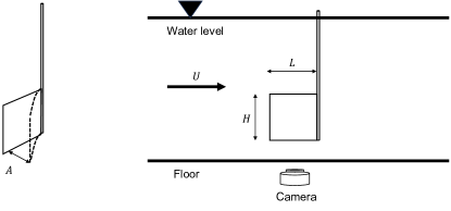
The dynamics of a conventional flag with a clamped leading edge in uniform flow, a classic fluid-structure interaction system, have been widely studied (see the review paper by Shelley & Zhang (2011)). The inverted variant of the same setup, with the trailing edge clamped has also gained significant interest recently. Figure 1 illustrates the latter configuration for the inverted flag.

Kim et al. (2013) experimentally showed that in both air and water flow, the amplitude dynamics of an inverted flag exhibit three main regimes: a stable undeformed regime, a large-amplitude oscillatory regime (flapping), and a fully deflected regime. These dynamics depend on the Reynolds number, the fluid-to-flag mass ratio $\mu_{\rho}$ and the dimensionless bending stiffness $K_{B}$. These parameters are defined as

$$Re=\frac{\rho_{f}UL}{\mu},\qquad\mu_{\rho}=\frac{\rho_{s}h}{\rho_{f}L},\qquad K_{B}=\frac{B}{\rho_{f}U^{2}L^{3}},$$ (1)

where $\rho_{f}$ and $\rho_{s}$ are the densities of the fluid and the elastic sheet the flag is made of; $U$ is the free stream velocity; $H$ and $L$ are the height and the length of the sheet, respectively; $h$ is the thickness of the sheet; $\mu$ is the viscosity of the fluid; and $B=Eh^{3}/12\left(1-\nu^{2}\right)$ is the bending rigidity of the sheet with $E$ and $\nu$ denoting Young’s modulus and Poisson’s ratio. This non-dimensional stiffness $K_{B}$ quantifies the magnitude of the flag’s elastic response to the deformation caused by the fluid flow.

In addition to the three dynamical regimes already mentioned, Ryu et al. (2015) numerically identified an intermediate regime, the deformed equilibrium, between the flapping mode and the undeformed equilibrium, which was confirmed by Yu et al. (2017) in experiments. Gurugubelli & Jaiman (2015) demonstrated that an inverted flag can generate significantly more strain energy than a conventional flag. Motivated by this finding, Shoele & Mittal (2016) explored the application of an inverted piezoelectric flag in energy harvesting. Sader et al. (2016) conducted experiments at Reynolds number $Re=\mathcal{O}(10^{4}-10^{5})$ and found that flapping is predominantly periodic but transitions to chaos as the flow speed increases.

Goza et al. (2018) characterized the chaotic flapping regime from simulations for a much lower Reynolds number $Re=\mathcal{O}(10^{2})$. Chaotic flapping develops when the stiffness is smaller than for the large-amplitude flapping regime, but not yet small enough for the totally deflected regime. They also conducted a stability analysis of the fully coupled equations and found that as $K_{B}$ decreases, the deformed equilibrium state undergoes a supercritical Hopf bifurcation to small-deflection deformed flapping. As $K_{B}$ decreases further, large amplitude flapping sets in. They predicted two unstable deflected equilibria for the flag in addition to its trivial unstable equilibrium corresponding to the undeflected state, as also obtained by the simplified phenomenological model of Sader et al. (2016).

While previous studies have offered great insight by analyzing extensive experimental and numerical data, it is desirable to model the behavior of such a nonlinear system including its various states and the transitions between them based on limited observations. Reduced-order modeling approaches have not yet been explored for the inverted flag setup. We therefore use the recently developed theory of spectral submanifolds (SSMs) to obtain a two-dimensional, data-driven model for the inverted flag directly from experimental data. SSMs are continuations of a spectral subspace of the linearized system near a stationary state such as a fixed point, a periodic orbit, or a quasiperiodic torus (Haller & Ponsioen, 2016). Initially, only the smoothest SSMs of stable stationary states and their reduced dynamics were constructed via Taylor-expansions. More recently, Haller et al. (2023) extended the theory to include secondary SSMs of limited smoothness (fractional SSMs) as well as SSMs tangent to eigenmodes of mixed stability type (mixed mode SSMs). We will use the dynamics on an attracting mixed-mode SSM as a reduced order model for the inverted flag.

In the large-amplitude flapping regime there are three unstable fixed points together with the limit cycle motion. They are all coexisting stationary states of the system. Under nonresonance conditions, SSM theory establishes the existence and uniqueness of SSMs attached to the middle equilibrium point. We show that the two deflected unstable equilibria and the stable limit cycle predicted by previous numerical studies and phenomenological models are all contained in this mixed-mode SSM. This enables us to derive a simple 2D data driven-model that captures all stable and unstable steady states of the flag as well as transitions among them.

In section 2 we describe our experimental setup and give a brief overview of data-driven model reduction to SSMs. In section 3, we apply SSM-reduction to our experimental data at two different Reynolds numbers to obtain a single 2D model for all stable and unstable steady states of the inverted flag. In section 4, we present our conclusions.

2 Experimental setup and nonlinear model reduction method

2.1 Experimental apparatus and procedure

We carry out our experiments in a recirculating open channel facility. A contraction ensures laminar flow entering the $2.4\mathrm{~{}m}$ long, $0.45\mathrm{~{}m}$ wide test section, filled with water to a depth of $0.41\mathrm{~{}m}$. We conduct experiments using two flags of different bending rigidity in different ranges of flow velocities, as summarized in table 1. These yield two Reynolds numbers, $Re=6\times 10^{4}$ and $Re=10^{5}$, defined at the velocity at which the large-amplitude periodic flapping have been modeled. The flags consist of polycarbonate sheets (Young’s modulus $E=2.38\times 10^{9}~{}Pa$, Poisson ratio $\nu=0.38$, density $\rho=1.2\times 10^{3}~{}kg\cdot m^{-3}$) clamped on an aluminum beam, 16 mm in diameter and rigidly mounted to the body of the channel. A schematic of the setup is shown in Fig. 1. The motion of the bottom tip of the flag, marked with a small color strip, is captured by a digital camera (4 Megapixels, 120 fps) through the transparent floor, a black cover on the test section serving as background. Beside the deflection $A$, we evaluate the velocity $\dot{A}$ after applying a Gaussian filter to the position data. The uncertainty on the latter, due to finite imaging resolution and small bending of the beam, is estimated as 1% of the total length of the flag. We conducted two types of experiments to characterize both the steady-state and the transient dynamics. For the former, we analyze the behavior after initial transients have dissipated, while the latter involve releasing the flag from various deflected positions with zero initial velocity.

Figure 1: Schematic view of the system with the water tunnel, linear actuator and the camera system. The flag’s length is $L$, height $H$, thickness $h$ and the tip’s deflection from its undeformed equilibrium position is denoted by $A$. Since the flapping is symmetric, we choose one side to be positive and other side to be negative in sign.

parameter	$Re=10^{5}$	$Re=6\times 10^{4}$
$L$	$150\ mm$	$150\ mm$
$H$	$150\ mm$	$150\ mm$
$h$	$1.5\ mm$	$0.8\ mm$
$U$	$1.0\ m/s$	$0.41\ m/s$
$\mu_{\rho}$	$0.012$	$0.0064$

Table 1: Flag properties in the two experiments; We used the same material, polycarbonate, for all experiments such that Young’s modulus, density and Poisson’s ratio remain the same. $U$ is the free stream velocity at which the periodic flapping behavior has been modeled.

2.2 Spectral submanifolds (SSMs) and data-driven reduced modeling of the flag dynamics

The considered system is infinite-dimensional, being governed by the coupled Navier-Stokes and Euler-Bernoulli partial differential equations (PDEs) for the fluid and solid, respectively. These are discretized to achieve a system of ordinary differential equations (ODEs) in the form:

$$\dot{\boldsymbol{x}}=\mathsfbi{A}\boldsymbol{x}+\boldsymbol{f}_{nl}(\boldsymbol{x}),\quad\boldsymbol{x}\in\mathbb{R}^{n},\quad\boldsymbol{f}_{nl}=\mathcal{O}(\left|\boldsymbol{x}\right|^{2})\in C^{\infty}.$$ (2)

The linearization of this system around its $\boldsymbol{x}=\boldsymbol{0}$ equilibrium is governed by the operator $\boldsymbol{A}$. Let $\lambda_{1},...,\lambda_{n}\in\mathbb{C}$ denote the eigenvalues of $\boldsymbol{A}$. If these eigenvalues satisfy the nonresonance condition

$$\sum_{j=1}^{n}m_{j}\lambda_{j}\neq\lambda_{k},\quad m_{j}\in\mathbb{N},$$ (3)

for $k=1,...,n$ and for all non-negative integers $m_{j}$ with $\sum_{j=1}^{n}m_{j}\geq 2$, system (2) can be exactly linearized via a $C^{\infty}$ change of coordinates near $\boldsymbol{x}=\boldsymbol{0}$ (see Sternberg (1958)). This implies that any spectral subspace $\mathcal{E}$ (i.e., any span of generalized eigenspaces) of $\boldsymbol{A}$ gives rise to a $C^{\infty}$ submanifold (SSM) $\mathcal{W}(\mathcal{E})$ for the nonlinear system (2) near the origin (Haller et al., 2023). $\mathcal{E}$ is called a like-mode spectral subspace if the signs of the real parts of all $\lambda_{j}$ inside $\mathcal{E}$ are the same, and $\mathcal{E}$ is called a mixed-mode spectral subspace otherwise. Similarly, the SSM $\mathcal{W}(\mathcal{E})$ is called a like-mode SSM if the associated $\mathcal{E}$ is like-mode spectral subspace, and $\mathcal{W}(\mathcal{E})$ is called a mixed-mode SSM otherwise.

This $\mathcal{W}(\mathcal{E})$ is an invariant manifold tangent to $\mathcal{E}$ at $\boldsymbol{x}=\boldsymbol{0}$ and has the same dimension as $\mathcal{E}$. If all eigenvalues of $\boldsymbol{A}$ outside $\mathcal{E}$ have negative real parts, then $\mathcal{W}(\mathcal{E})$ is an attracting invariant manifold to which all neighbouring trajectories converge exponentially fast. In that sense, the dynamics on $\mathcal{W}(\mathcal{E})$ serves as a reduced-order model with which all nearby trajectories synchronize exponentially fast.

Applications of SSM-based model reduction to mechanical systems have been discussed by Haller & Ponsioen (2017); Breunung & Haller (2018); Haller & Ponsioen (2016); Ponsioen et al. (2018, 2020); Jain et al. (2018); Jain & Haller (2022). Recently, a data-driven approach to SSM-reduction has been developed and a corresponding MATLAB package has been released by Cenedese et al. (2022a, b). As noted in Cenedese et al. (2022a), if observations of the full state space variable $\boldsymbol{x}$ are not available, one can use delay-embedding of a smaller set of observables to reconstruct SSMs based on Takens’s embedding theorem (Takens, 1981). Under appropriate nondegeneracy conditions, this theorem guarantees that an $m$-dimensional invariant manifold of system (2) can be smoothly embedded into a generic observable space of dimension $p\geq 2m+1$.

In the case of the inverted flag, the tip displacement $A(t)$ can be used to define a delay-embedded observable vector $\mathbf{y}(t)=(A(t),A(t+\Delta t),...,A(t+(p-1)\Delta t))\in\mathbb{R}^{p}$. The SSM $\mathcal{W}(\mathcal{E})$ we seek to reconstruct in the space of this observable is the slowest SSM of the unstable fixed point corresponding to the undeflected position of the flag. This two-dimensional SSM is tangent to the spectral subspace of the linearized dynamics that is spanned by the eigenvectors of a positive and a negative real eigenvalue. By Takens’s theorem, the dimension of the observable space should be at least $p=5$, given that the dimension of the SSM is $m=2$.

To construct the parametrization of the two-dimensional SSM $\mathcal{W}(\mathcal{E})$ in the observable space, we follow the procedure developed by Cenedese et al. (2022a). Let $\mathbf{W}_{0}\in\mathbb{R}^{2\times p}$ be the matrix composed of the a priori unknown vectors spanning the tangent space $\mathcal{E}$ of $\mathcal{W}(\mathcal{E})$ at the origin. We approximate $\mathbf{W}_{0}$ from singular value decomposition of trajectory segments passing by the undeflected position of the flag. Specifically, $\mathbf{W}_{0}$ is chosen as the span of the two leading singular vectors of the trajectory data matrix constructed for the observable $\mathbf{y}(t)$. Reduced coordinates on $\mathcal{E}$ can be defined as $\boldsymbol{\eta}=\mathbf{W}_{0}\mathbf{y}$, i.e. the projection of the observable coordinates onto $\mathcal{E}$. We aim to parametrize the SSM $\mathcal{W}(\mathcal{E})$ as a polynomial function $\boldsymbol{y}=\mathbf{V}_{0}\boldsymbol{\eta}+\mathbf{V}\boldsymbol{\eta}^{2:l}$, where the vector $\boldsymbol{\eta}^{2:l}$ contains all scalar monomials of the variables $\eta_{1}$ and $\eta_{2}$ from degree $2$ to $l$ and $\mathbf{W}_{0}\mathbf{V}_{0}=\mathbf{I}$. Delay-embedded slow SSMs are nearly flat near the origin as deduced in general by Cenedese et al. (2022a). Based on this observation, we set $\mathbf{V}=\mathbf{0}$.

We then look for the reduced dynamics on the SSM $\mathcal{W}(\mathcal{E})$ as the projection of the full dynamics in the observable space. We use polynomials up to $M$-th order to represent the dynamics on $\mathcal{W}(\mathcal{E})$ in reduced coordinates:

$$\begin{gathered}\dot{\boldsymbol{\eta}}=\mathbf{R}_{0}\boldsymbol{\eta}+\mathbf{R}\boldsymbol{\eta}^{2:M},\\ \boldsymbol{\eta}=(\eta_{1},\eta_{2})^{T}\in\mathbb{R}^{2}.\end{gathered}$$ (4)

To learn $\mathbf{R}_{0}$ and $\mathbf{R}$ from the data set of $K$ experiments $\mathbf{y}_{1},\ldots,\mathbf{y}_{K}$, we first project them to $\mathcal{W}(\mathcal{E})$ in a direction orthogonal to $\mathcal{E}$ to obtain $\boldsymbol{\eta}_{1},\ldots,\boldsymbol{\eta}_{K}$. We obtain the time derivatives $\dot{\boldsymbol{\eta}}$ via numerical differentiation and formulate a minimization problem to find the best fitting matrices $(\mathbf{R}_{0}^{*},\mathbf{R}^{*})$ in formula (4) using the cost function

$$\begin{gathered}\left(\mathbf{R}_{0}^{*},\mathbf{R}^{*}\right)=\arg\min_{\mathbf{R}_{0},\mathbf{R}}\sum_{j=1}^{K}\left\|\dot{\boldsymbol{\eta}}_{j}-\mathbf{R}_{0}\boldsymbol{\eta}_{j}-\mathbf{R}\boldsymbol{\eta}_{j}^{2:M}\right\|^{2}.\end{gathered}$$ (5)

Among all the dynamic regimes, large-amplitude flapping tends to generate the most interest as it results in large strain energy suitable for energy harvesting. Our objective is to find the slow SSM of the undeformed state with its reduced dynamics in order to model all coexisting stationary states (deformed equilibria on two sides, undeformed equilibrium in the middle and a stable limit cycle), as well as transition orbits among them.

3 Results

3.1 Dynamical regimes of an inverted flag

Previous findings indicate that as the stiffness $K_{B}$ decreases, the flag experiences a sequence of different dynamic regimes, as discussed in the Introduction. Starting with an undeformed static equilibrium, it progresses through small deflections, small-amplitude flapping, large-amplitude flapping, chaotic flapping, and finally, fully deflected state with the free end pointing downstream as a conventional flag. Kim et al. (2013) and Yu et al. (2017) report qualitatively similar bifurcation diagrams after comparing results from water and wind tunnels. In our experiments, we focus on mass ratio $\rho_{s}h/\rho_{f}L=\mathcal{O}(10^{-2})$ and aspect-ratio $H/L=1$.

We plot the tip displacements against the stiffness $1/K_{B}$ to construct the bifurcation diagram for the flag. Following Goza et al. (2018) and Tavallaeinejad et al. (2021), we construct a Poincaré-section based on the tip velocity crossing zero.

As shown in Fig. 2, the bifurcation diagrams for both investigated $Re$ are quantitatively similar. This aligns with the findings of Sader et al. (2016), that the flapping dynamics regimes are insensitive to changes in $Re$. We find that the first bifurcation leading to large amplitude flapping occurs for $0.18\leq K_{B}\leq 0.25$ at $Re=6\times 10^{4}$ and for $0.16\leq K_{B}\leq 0.25$ at $Re=10^{5}$. This is consitent with the experiments by Kim et al. (2013) who observed such bifurcation for $0.2\leq K_{B}\leq 0.25$ at a similar mass ratio.

Figure 2: Bifurcation diagrams of the inverted flag as a function of stiffness. Under decreasing stiffness $K_{B}$, the flag experiences a sequence of different dynamic regimes, as seen in the plots. (a) $Re=6\times 10^{4}$ and (b) $Re=10^{5}$

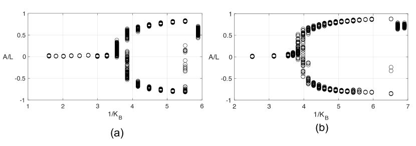
We observe that under decreasing stiffness $K_{B}$, the inverted flag explores the same dynamic regimes that have been reported by others, as stated in the Introduction. Specifically, we note that the flag stretches straight in the stable undeformed equilibrium, then buckles with small deflections at a stable deflected equilibrium, progresses to small-amplitude asymmetric deformed flapping and then large-amplitude flapping. Chaotic behavior is also observed before the flag ultimately becomes fully deflected.

3.2 The reduced order model constructed at $Re=6\times 10^{4}$

Having explored the dynamical regimes of the inverted flag, we now seek to find an SSM-reduced model in the large-amplitude flapping regime using the data-driven SSMLearn methodology of Cenedese et al. (2022a). We obtain the necessary transient trajectories from experiments initialized with nonzero deflection and zero velocity at $Re=6\times 10^{4}$. We apply delay-embedding to the tip displacement time-series to represent the trajectories in the observable space. The processed trajectories are shown in Fig. 3a. To discover the dynamics in a larger subset of the observable space, we choose the initial deflections of the flag in the range of large-amplitude deflection, especially near the three fixed points.

Figure 3: (a) Eight sample trajectories collected during the transient experiments. They show transient dynamics before settling down to the stable limit cycle oscillation. (b) Trajectories in the reduced coordinates and the SSM (pink) obtained using the training data. Here $\eta_{1}$ and $\eta_{2}$ are the reduced coordinates and the vertical axis denotes the amplitude of the tip deflection. (c) A snapshot of the experimental video. The blue line indicates the undeflected position of the flag; a white circle shows the position of the tip of the flag, the tip deflection is represented by the red arrow.

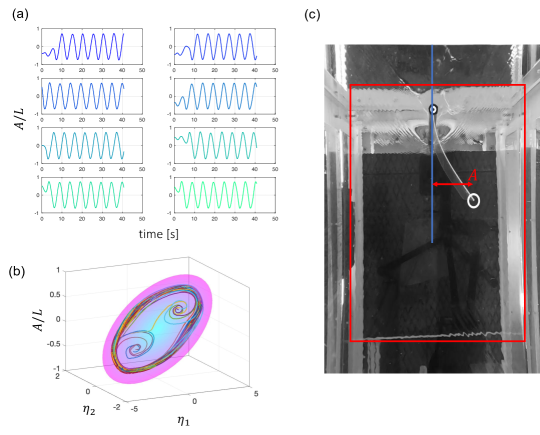
The undeformed equilibrium is known to become an unstable saddle-type fixed point via a supercritical pitchfork bifurcation (Tavallaeinejad et al., 2021) of the deformed equilibrium. Its two slowest eigenvalues are real, with one being positive and the other negative. The non-resonance condition (3) generally holds for a physical system that has dissipation, especially in a data-driven setting for real-world experiments. Therefore, we fit a two-dimensional mixed-mode SSM to the experimental data, as the associated spectral subspace $\mathcal{E}$ contains eigenvalues with different signs. We first divide the collected trajectories into a training set and a test set. The training set is used to construct $\mathcal{W}(\mathcal{E})$ from singular valued decomposition and its reduced dynamics (4) by solving the optimization problem (5). The test set is reserved to evaluate the performance of the SSM-based model. In total, we collect 20 trajectories, 4 of which are reserved for testing and 16 are used for training. In Fig. 3a-b, we show the training data we use together with the two-dimensional SSM $\mathcal{W}(\mathcal{E})$.

After extracting the SSM $\mathcal{W}(\mathcal{E})$ from the training data, we project the trajectories of the training set in the observable space on $\mathcal{W}(\mathcal{E})$ and use the general polynomial form in Eq.(4) to find the best fitting reduced dynamics. To determine parameters for the polynomial regression, such as the embedding dimension $p$ and the order of the polynomial $M$ to fit the reduced dynamics, a grid search method is employed to minimize the reconstruction error on the training data set, as illustrated in Cenedese et al. (2022a). We use non-regularized polynomial regression. For the embedding dimension, we choose $p=25$ and for the polynomial order, we select $M=11$ in (4) after the grid search.

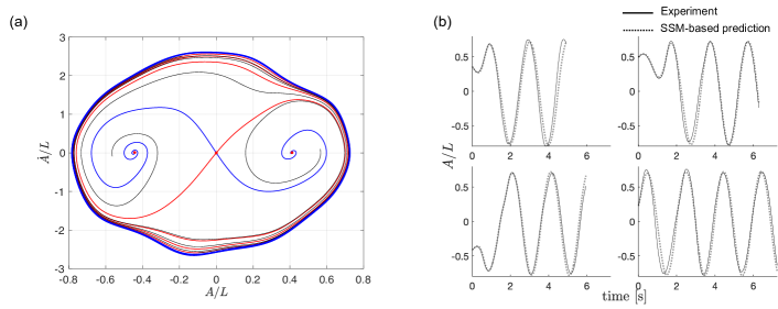
The reduced-order model (4) is a planar dynamical system. Inspection of the vector field defining the right-hand side of this model ODE reveals three coexisting unstable fixed points and a stable limit cycle. Physically, the fixed points capture two deformed unstable equilibira in symmetric positions and one undeformed equilibrium in the middle. These findings confirm the numerically predicted unstable fixed points of Goza et al. (2018), and also uncover the geometry of transitions from these fixed points to the stable limit cycle describing the large-amplitude flapping of the flag. Note that we have not used any knowledge of the existence of the unstable deflected fixed points and the limit cycle: they were discovered from a model obtained using general trajectories. This shows the predictive power of our SSM-based reduced order model.

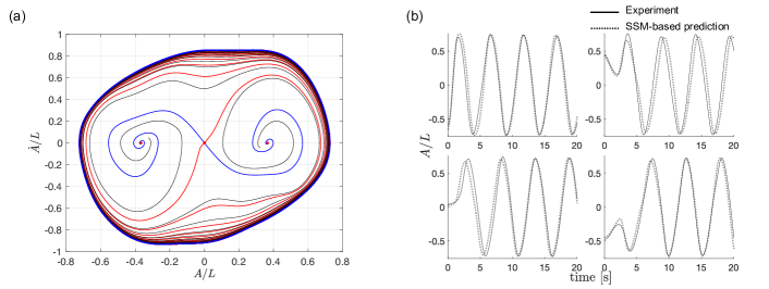
Our low-dimensional model is also geometrically interpretable. The phase portrait of the planar system is influenced by the fixed points and their stable and unstable manifolds that we can find by time integration of the model. We initialize trajectories close to the three fixed points and advect them with the reduced model. We then transform the trajectories to the observable space and obtain the corresponding tip displacements as well as velocities. This results in a phase portrait purely in terms of physical variables, as shown in Fig. 4a. The heteroclinic orbits that connect the undeformed equilibrium with the deformed equilibria are shown in blue lines.

To examine the predictive power of our SSM-reduced model more closely, we reconstruct the test set. By running the SSM-reduced model on the same initial conditions numerically, we can advect the predicted trajectory, transform to the observable space and compare the predicted and the actual tip displacements. Figure 4b shows the predictions of the model as well as the experimental data, which are in close agreement.

Figure 4: (a) The nonlinear phase portrait in the tip displacement and velocity coordinates at $Re=6\times 10^{4}$. The red curve represents the unstable manifold, while the blue curve denotes the stable manifold of the undeformed state. The closed blue curve on the exterior shows the limit cycle, with two black curves depicting trajectories initialized near unstable deformed equilibria. Three fixed points are shown in red dots. (b) Our predictions of the tip motion versus the test trajectories at $Re=6\times 10^{4}$. The label ”Experiment” refers to the experimentally measured test trajectories, while ”Prediction” refers to predictions by the SSM-reduced model.

3.3 The reduced order model constructed at $Re=10^{5}$

In order to investigate the effect of the change in Reynolds number on the SSM-reduced model, we also perform the same experiments as in section 3.2 at $Re=10^{5}$. At this Reynolds number, a total of 17 transient trajectories are collected of which 13 are used for training and 4 for testing.

Since the data set at this Reynolds number is intrinsically different from the one at lower Reynolds number, we perform again a grid search on the training data to determine the optimal values for $p$ and $M$. The dimension of the manifold remains two as the spectral subspace $\mathcal{E}$ has the same dimension and stability type. Based on a minimization of the trajectory reconstruction error, we chose the dimension of the observable space $p=9$ and the polynomial order $M=11$ in (4) after the grid search.

We construct the phase portrait in the same way as before, by releasing initial conditions near the three fixed points and integrating the reduced model. Then we transform the trajectories back to the tip displacements and velocities shown in Fig. 5a. The SSM at higher Reynolds number also contains three unstable fixed points and one stable limit cycle. The reconstructed trajectories are obtained by integrating the model from the initial conditions of the test set. As shown in Fig. 5b, we again obtain accurate predictions over the test data set. Therefore the predictive power of our SSM-reduced model does not change as we double the Reynolds number.

Figure 5: Same as Fig. 4 but for $Re=10^{5}$.

4 Conclusion

In this paper, we have constructed a nonlinear reduced-order model for an inverted flag from experimental data collected in its large amplitude flapping regime. We have performed experiments to construct the canonical bifurcation diagram of the inverted flag that aligns with those reported in the literature. We have demonstrated that SSM-reduced nonlinear models can capture three coexisting unstable fixed points and a stable limit cycle, as well as the transitions between those. We start with the undeformed unstable equilibrium as our anchor point and discover the other two unstable fixed points. Although these unstable fixed points were predicted in the literature from numerical simulation by Goza et al. (2018), our reduced-order model did not utilize this information. Additionally, our SSM-reduced model has also provided reliable predictions for transitions between those states, which have been unexplored in prior studies. In particular, we observe that initial conditions in the neighborhood of either one of the deformed states synchronize with the limit cycle dynamics, but their oscillations are in anti-phase, as evidenced by the black curves of Fig. 4a and Fig. 5a. These types of orbits take the longest time to converge to the limit cycle. We have also found heteroclinic orbits connecting the undeformed equilibrium with the deformed states. We have finally confirmed that the system is not sensitive to changes in Reynolds number in the considered regime, $Re=\mathcal{O}(10^{4}-10^{5})$.

The two-dimensional, SSM-reduced polynomial model we have obtained creates an opportunity to design a closed-loop controller for the inverted flag. A possible actuation mechanism is the rotation of the trailing edge of the flag, as pursued by Tang & Dowell (2013) in a different setting. Possible control objectives range from the stabilization or elimination of select unstable equilibria or the reduction or enhancement of the limit cycle amplitude to a desired level. Building on the recent SSM-reduced control methodology used in model-predictive control of soft robots (Alora et al., 2023a, b), the development of a closed-loop, SSM-reduced controllers for the inverted flag is currently underway.

References

- Alora et al. (2023a) Alora, J. I., Cenedese, M., Schmerling, E., Haller, G. & Pavone, M. 2023a Data-Driven Spectral Submanifold Reduction for Nonlinear Optimal Control of High-Dimensional Robots. In IEEE Int. Conf. Robot., pp. 2627–2633.
- Alora et al. (2023b) Alora, J. I., Cenedese, M., Schmerling, E., Haller, G. & Pavone, M. 2023b Practical Deployment of Spectral Submanifold Reduction for Optimal Control of High-Dimensional Systems. IFAC-PapersOnLine 56 (2), 4074–4081.
- Breunung & Haller (2018) Breunung, T. & Haller, G. 2018 Explicit backbone curves from spectral submanifolds of forced-damped nonlinear mechanical systems. Proc. Math. Phys. Eng 474 (2213), 20180083.
- Cenedese et al. (2022a) Cenedese, M., Axås, J., Bäuerlein, B., Avila, K. & Haller, G. 2022a Data-driven modeling and prediction of non-linearizable dynamics via spectral submanifolds. Nat. Commun. 13 (1), 872.
- Cenedese et al. (2022b) Cenedese, M., Axås, J., Yang, H., Eriten, M. & Haller, G. 2022b Data-driven nonlinear model reduction to spectral submanifolds in mechanical systems. Philos. Trans. Royal Soc. A 380 (2229), 20210194.
- Dowell & Hall (2001) Dowell, E. H. & Hall, K. C. 2001 Modeling of fluid-structure interaction. Annu. Rev. Fluid Mech. 33 (1), 445–490.
- Goza et al. (2018) Goza, A., Colonius, T. & Sader, J. E. 2018 Global modes and nonlinear analysis of inverted-flag flapping. J. Fluid Mech. 857, 312–344.
- Gurugubelli & Jaiman (2015) Gurugubelli, P. S. & Jaiman, R. K. 2015 Self-induced flapping dynamics of a flexible inverted foil in a uniform flow. J. Fluid Mech. 781, 657–694.
- Haller et al. (2023) Haller, G., Kaszás, B., Liu, A. & Axås, J. 2023 Nonlinear model reduction to fractional and mixed-mode spectral submanifolds. Chaos 33 (6), 063138.
- Haller & Ponsioen (2016) Haller, G. & Ponsioen, S. 2016 Nonlinear normal modes and spectral submanifolds: existence, uniqueness and use in model reduction. Nonlinear Dyn. 86 (3), 1493–1534.
- Haller & Ponsioen (2017) Haller, G. & Ponsioen, S. 2017 Exact model reduction by a slow–fast decomposition of nonlinear mechanical systems. Nonlinear Dyn. 90 (1), 617–647.
- Holmes et al. (1996) Holmes, P., Lumley, J. L. & Berkooz, G. 1996 Turbulence, Coherent Structures, Dynamical Systems and Symmetry. Cambridge Monographs on Mechanics . Cambridge University Press.
- Hsu & Bazilevs (2012) Hsu, MC. & Bazilevs, Y. 2012 Fluid–structure interaction modeling of wind turbines: simulating the full machine. Comput. Mech. 50, 821–833.
- Jain & Haller (2022) Jain, S. & Haller, G. 2022 How to compute invariant manifolds and their reduced dynamics in high-dimensional finite element models. Nonlinear Dyn. 107 (2), 1417–1450.
- Jain et al. (2018) Jain, S., Tiso, P. & Haller, G. 2018 Exact nonlinear model reduction for a von Kármán beam: Slow-fast decomposition and spectral submanifolds. J. Sound Vib. 423, 195–211.
- Kaszás & Haller (2024) Kaszás, B. & Haller, G. 2024 Capturing the edge of chaos as a spectral submanifold in pipe flows. J. Fluid Mech. 979, A48.
- Kim et al. (2013) Kim, D., Cossé, J., Cerdeira, C. H. & Gharib, M. 2013 Flapping dynamics of an inverted flag. J. Fluid Mech. 736.
- de Langre E. (2008) de Langre E. 2008 Effects of Wind on Plants. Annu. Rev. Fluid Mech. 40 (1), 141–168.
- Linot & Graham (2020) Linot, A. J. & Graham, M. D. 2020 Deep learning to discover and predict dynamics on an inertial manifold. Phys. Rev. E 101, 062209.
- Page & Kerswell (2019) Page, J. & Kerswell, R. R. 2019 Koopman mode expansions between simple invariant solutions. J. Fluid Mech. 879, 1–27.
- Ponsioen et al. (2020) Ponsioen, S., Jain, S. & Haller, G. 2020 Model reduction to spectral submanifolds and forced-response calculation in high-dimensional mechanical systems. J. Sound Vib. 488, 115640.
- Ponsioen et al. (2018) Ponsioen, S., Pedergnana, T. & Haller, G. 2018 Automated computation of autonomous spectral submanifolds for nonlinear modal analysis. J. Sound Vib. 420, 269–295.
- Ryu et al. (2015) Ryu, J., Park, S. G., Kim, B. & Sung, H. J. 2015 Flapping dynamics of an inverted flag in a uniform flow. J. Fluids Struct. 57, 159–169.
- Sader et al. (2016) Sader, J. E., Cossé, J., Kim, D., Fan, B. & Gharib, M. 2016 Large-amplitude flapping of an inverted flag in a uniform steady flow–a vortex-induced vibration. J. Fluid Mech. 793, 524–555.
- Schmid (2022) Schmid, P. J. 2022 Dynamic Mode Decomposition and Its Variants. Annu. Rev. Fluid Mech. 54 (1), 225–254.
- Shelley & Zhang (2011) Shelley, M. J. & Zhang, J. 2011 Flapping and Bending Bodies Interacting with Fluid Flows. Annu. Rev. Fluid Mech. 43 (1), 449–465.
- Shoele & Mittal (2016) Shoele, K. & Mittal, R. 2016 Energy harvesting by flow-induced flutter in a simple model of an inverted piezoelectric flag. J. Fluid Mech. 790, 582–606.
- Sternberg (1958) Sternberg, Shlomo 1958 On the Structure of Local Homeomorphisms of Euclidean n-Space, II. Am. J. Math. 80 (3), 623–631.
- Takens (1981) Takens, F. 1981 Detecting strange attractors in turbulence. In Dynamical Systems and Turbulence, Warwick 1980 (ed. David Rand & Lai-Sang Young), pp. 366–381. Berlin, Heidelberg: Springer Berlin Heidelberg.
- Tang & Dowell (2013) Tang, D. & Dowell, E. H. 2013 Computational/experimental aeroelastic study for a horizontal-tail model with free play. AIAA J. 51, 341–352.
- Tavallaeinejad et al. (2021) Tavallaeinejad, M., Salinas, M. F., Païdoussis, M. P., Legrand, M., Kheiri, M. & Botez, R. M. 2021 Dynamics of inverted flags: Experiments and comparison with theory. J Fluids Struct. 101, 103199.
- Yu et al. (2017) Yu, Y., Liu, Y. & Chen, Y. 2017 Vortex dynamics behind a self-oscillating inverted flag placed in a channel flow: Time-resolved particle image velocimetry measurements. Phys. Fluids 29 (12), 125104.