Defect versus defect: phases of single file marching in periodic landscapes with road blocks

Abstract

We consider an inhomogeneous asymmetric exclusion processes in a closed geometry with a point and an extended defects across which the hopping rates are less than elsewhere. We study the stationary density profiles that result from the competition between the point and extended defects. By using a minimum current principle, we identify the conditions of the existence of a localised shock or a localised domain wall. We further elucidate delocalisation of these localised domain walls, when the strengths of the point and extended defects follow a certain mutual relationship, which originates again from the minimum current principle. We show that in that case the system admits a pair of delocalised domain walls, none of which can penetrate the extended defect. We calculate the fluctuation properties of the domain walls and obtain the long time averaged shapes of the delocalised domain walls.

I Introduction

Totally asymmetric simple exclusion process (TASEP) with open boundaries and its related models in one dimension (1D) serve as simple models of restricted 1D transport. TASEP was originally introduced as a simple model describe ribosome translocation along messenger RNA in eukaryotic cells macdonald1 . TASEP has been used to describe a varieties of physical systems, e.g., fluid motion along artificial crystalline zeolitical structures fluid and movement of unidirectional vehicular traffic along roads traffic . It was subsequently discovered to have novel boundary induced phase transitions tasep1 ; tasep2 . See Refs. rev1 ; rev2 for reviews on TASEP. Natural systems are never pure. Impurities or defects are ever present in condensed matter or biological systems. In a TASEP, this can be in the form of a point or a finite fraction of the channel (called an “extended defect”) having reduced hopping rates that tend to hamper flow of particles. Open TASEPs with both point and extended defects have been studied previously; see, e.g., Refs. def1 ; def2 ; def3 ; def4 ; def5 . TASEP with periodic boundary conditions that necessarily conserved total particle number has also been studied. A uniform TASEP on a ring necessarily has a spatially uniform mean density in the steady states, due to the underlying translational invariance. In contrast, an inhomogeneous TASEP in a ring geometry explicitly breaks the translational invariance, and hence is a candidate to produce macroscopically nonuniform steady state densities. For instance, studies on TASEP in a ring geometry with either one lebo or two niladri-tasep point defects reveal spatially nonuniform stationary densities when the mean particle is intermediate, i.e., neither too low (close to zero), nor too high (close to unity), the TASEP admits localised (LDW) or delocalised (DDW) domain walls. Similarly, a periodic TASEP with one or more extended defects can display one LDW mustansir or more than one DDWs tirtha-niladri for intermediate mean densities. For sufficiently low or high densities, the bulk density is macroscopically uniform, independent of whether the defects in question are point or extended. Thus defects tend to become controlling factors of the ensuing steady states in the systems when there are sufficient number of particles in the system.

An important issue concerning the role of defects in TASEP is the interplay and competition between multiple defects of different types that result into nonuniform steady states in the TASEP. Being motivated by this generic issue, we here study a periodic TASEP having one point defect and one extended defect. Apart from its theoretical motivations, this study would be useful to understand the phenomenologies of ribosome translocations along closed mRNA loops (circular translation of polysomal mRNA) with clusters of slow codons along which ribosome translocations are inhibited mrna1 ; mrna11 ; mrna2 ; mrna3 ; mrna4 ; mrna5 . The principal result from our work is that for intermediate values of the mean density, both there can be an LDW due to both the point and extended defects. This leads to competition between them. We invoke a minimum current principle to decide the dominant defect. Furthermore, when the strengths (defined below) of the point and extended defects maintain a particular relation, for intermediate densities one find a pair of DDWs instead of a single LDW. For very low and high densities, LD and HD phases follow.

II Model

We consider an inhomogeneous asymmetric exclusion process in a ring geometry with $L$ sites; see Fig. 1 for a schematic diagram of the model. The model has a single slow site at $i=1$ and an extended slow section from $i=\epsilon_{1}\,L$ to $(\epsilon_{1}+\epsilon_{2})L,\,\epsilon_{1},\epsilon_{2}<1$. The hopping rate across the single slow site at $i=1$ is assumed to be $p<1$, and the extended slow segment has a hopping rate $q<1$. In general $p\neq q$. Elsewhere in the system, the hopping rate is unity. The particles are assumed move in the anticlockwise direction. Periodic boundary condition is imposed on the system. The following microscopic processes fully describe the dynamics of the model:

(a) At any site $i=1$ to $\epsilon_{1}\,L,\,\epsilon_{1}<1$, particles hop in an anticlockwise manner to the neighboring site at rate unity, subject to exclusion.

(b) At any site $i=\epsilon_{1}\,L$ to $(\epsilon_{1}+\epsilon_{2})L,\,\epsilon_{1}+\epsilon_{2}<1$, particles hop in an anticlockwise manner to the neighboring site at rate $q<1$, subject to exclusion.

(c) At any site $i=(\epsilon_{1}+\epsilon_{2})\,L$ to $i=L$, particles hop in an anticlockwise manner to the neighboring site at rate unity, subject to exclusion.

(d) From site $i=L$ to 1, particles hop in an anticlockwise manner to the neighboring site at rate $p<1$, subject to exclusion.

Figure 1: Schematic model diagram. The thick bluish green circle marks the point defect across which the hopping rate is $p<1$. The arc in red is the extended defect along which the hopping rate is $q<1$. In the remaining segments, the hopping rate is unity (see text).

III Steady state density profiles

III.1 Mean-field theory

In this Section, we set up and analyze the MFT equations. Let $n_{i}$ be the occupation at site $i$. In the MFT approximation, correlations are neglected and averages of products are replaced by products of averages blythe . While MFT is an adhoc approximation, it provides a good analytically tractable guideline to the steady state densities and phase diagrams. It is convenient to consider the system to be composed of three segments - $T_{1}$ between $i=1$ to $\epsilon_{1}L$,$T_{2}$ between $\epsilon_{1}L$ to $(\epsilon_{1}+\epsilon_{2})L$ and $T_{3}$ between $(\epsilon_{1}+\epsilon_{2})L$ to $L$, connected serially. The MFT equation for the density $n_{i}$ in the different segments reads

$$\frac{dn_{i}}{dt} = n_{i+1}[1-n_{i}]-n_{i}[1-n_{i-1}],\;1<i<\epsilon_{1}L,$$ (3)

$$= qn_{i+1}[1-n_{i}]-qn_{i}[1-n_{i-1}],$$

$$\;\;\;\;\;\;\epsilon_{1}L\leq i\leq(\epsilon_{1}+\epsilon_{2})L,$$

$$= n_{i+1}[1-n_{i}]-n_{i}[1-n_{i-1}],$$

$$\;\;\;\;\;\;(\epsilon_{1}+\epsilon_{2})L<i\leq L.$$

We note that the above mean-field equations are invariant under the transformations $n_{i}\rightarrow 1-n_{L-i-1}$, which defines the particle hole symmetry in this model. Before proceeding further it is convenient introduce a quasi-continuous coordinate $x\equiv i/L$ in the thermodynamic limit $L\rightarrow\infty$. Thus, we have $0\leq x\leq 1$. Now defining $\rho_{a}(x)\equiv\langle n^{a}_{i}\rangle$, where $\langle...\rangle$ implies temporal averages in the steady states and $a=1,\,2$ or $3$ for the three segments, the MFT equations in the steady states yield the stationary currents $J_{1},\,J_{2},\,J_{3}$ in the three segments as

$$J_{1} = \rho_{1}(1-\rho_{1}),$$ (4)

$$J_{2} = q\rho_{2}(1-\rho_{2}),$$ (5)

$$J_{3} = \rho_{3}(1-\rho_{3}),$$ (6)

where $\rho_{1},\,\rho_{2}$ and $\rho_{3}$ are the stationary densities in $T_{1},\,T_{2}$ and $T_{3}$ respectively. Current conservation means

$$J_{1}=J_{2}=J_{3}$$ (7)

in the steady states. Each of $T_{1},T_{2},T_{3}$ can be in its LD, HD, MC phase individually, similar to an open TASEP. In addition, they can also be in their domain wall (DW) phase. Furthermore, particle number conservation (PNC) gives

$$\int_{0}^{\epsilon_{1}}\rho_{1}dx+\int_{\epsilon_{1}}^{\epsilon_{1}+\epsilon_{2}}\rho_{2}dx+\int_{\epsilon_{2}+\epsilon_{1}}^{1}\rho_{3}dx=n,$$ (8)

where $n=\sum_{i}\,n_{i}/L$ is the mean particle density in the system.

Steady state currents (4)-(6) together with the particle number conservation (8) can be used to calculate the steady state densities $\rho_{1},\,\rho_{2},\,\rho_{3}$. A complete characterization of the steady states of this model requires specifying the phases in all of $T_{1},\,T_{2},\,T_{3}$, i.e., solving for all of $\rho_{1},\,\rho_{2},\,\rho_{3}$. While an open TASEP can be in LD, HD and MC phases, a TASEP in a closed system can be in domain wall (DW) phase in an extended region of the space of the control parameters lebo ; niladri-tasep ; mustansir ; hinsch ; tirtha-niladri ; parna-anjan ; astik-parna . While each of $T_{1},T_{2},T_{3}$ can be in any of these four phases under various conditions, we will see below that the conditions of current conservation and PNC ensure that not all of the phases are actually admissible in the present model. This forms a principal result from this work. In general, all of $T_{1},\,T_{2},\,T_{3}$ may be in the same phases, or different phases. We name the former as identical phase solutions and the latter as distinct phase solutions. Before we make detailed quantitative analysis, we can make the following general comments. We note that $J_{1}=J_{3}$ gives $\rho_{1}=\rho_{3}$ or $\rho_{1}=1-\rho_{3}$ in the steady state. We shall see below that the relation between $\rho_{2}$ and $\rho_{1}$ (or $\rho_{3}$) is more complex due to $q<1$.

In order to validate our mean-field theory, we have also performed stochastic simulations (using a random sequential update algorithm) to determine the phase diagrams and calculate the stationary densities, and we compare with our mean-field theory predictions; see Section III.6 for more details on the numerical simulations.

III.1.1 Identical phase solutions in MFT

We first explore the possibilities of all the three channels are in the same phase, which form the identical phase states of the system. In this case, the possible phases of the system are LD-LD-LD, HD-HD-HD and MC-MC-MC phases. We use (7) and (8) to determine the phases.

LD-LD-LD phase:- For sufficiently low mean densities $n$, all the channels should be sparsely populated, and hence we expect all the three segments to be in their LD phases with uniform densities $\rho_{1}=\rho_{3}<\rho_{2}<1/2$ respectively. These may be obtained as follows. By using $J_{1}=J_{2}=J_{3}$

$$\rho_{1}(1-\rho_{1})=q\rho_{2}(1-\rho_{2})=\rho_{3}(1-\rho_{3}).$$ (9)

Since $q<1$, we expect $\rho_{1}=\rho_{3}<\rho_{2}$ in the LD phase. Form (9), we get

$$\rho_{1}=\rho_{3}=\frac{1}{2}[1\pm\sqrt{1-4q\rho_{2}(1-\rho_{2})}].$$ (10)

Since we are looking for the LD-LD-LD phase, we choose

$$\rho_{1}=\rho_{3}=\frac{1}{2}[1-\sqrt{1-4q\rho_{2}(1-\rho_{2})}]<\frac{1}{2}.$$ (11)

Now using (8) we get

$$[1-\epsilon_{2}]\rho_{1}+\rho_{2}\epsilon_{2}=n<\frac{1}{2}$$ (12)

for the LD phase.

For explicit solutions of the densities in the LD-LD-LD phase, (9) together with (12) can be used to give

$$\rho_{1}=\left[-B\pm\sqrt{B^{2}-4AC}\right]\frac{1}{2A},$$ (13)

as the two general solutions, where

$$A = (1-\epsilon_{2})^{2}-\epsilon_{2}^{2}/q,$$ (14)

$$B = \frac{\epsilon_{2}^{2}}{q}-(1-\epsilon_{2})(2n-\epsilon_{2}),$$ (15)

$$C = n^{2}-\epsilon_{2}n.$$ (16)

So far we have not imposed any conditions of the LD-LD-LD phase on the solutions (13). The pertinent question then is: Which of the two solutions in (11) is to be considered as the LD-LD-LD phase density solution? To settle this, we use the fact that in the limiting case with vanishing particle number, i.e., with $n\rightarrow 0$, the LD-LD-LD phase solution must smoothly go to zero. This consideration allows us to pick the right solution in (13) for the LD-LD-LD phase: we choose the solution that vanishes as $n\rightarrow 0$. Which one among the two in (13) does that depends upon the signs of $A$ and $B$, i.e., will be decided by $\epsilon_{2}$ and $n$. We thus note that the point defect has no macroscopic effect on the steady state density profiles. Instead at $x=0$, the location of the point defect, there is a local peak of height $h$ and vanishing width in the thermodynamic limit, with $h=n(1-p)/p$, such that the local density at $x=0$ is $\rho_{1}+h$ niladri-tasep . This essentially acts as a boundary layer between $T_{1}$ and $T_{3}$. Steady state density profiles in the LD-LD-LD phase with $n=0.15,p=0.2,\,q=0.45$ and $n=0.15,p=0.15,\,q=0.6$ with a system size $L=9000$ and $\epsilon_{1}=\epsilon_{2}=1/3$ are shown in Fig. 2. Good agreement between MFT and MCS results are observed.

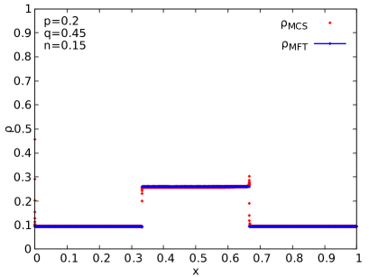
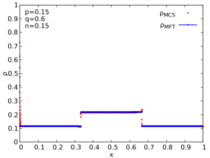
Figure 2: LD-LD-LD density plots with $n=0.15$: (top) $p=0.2,\,q=0.45$, (bottom) $p=0.15,\,q=0.6$. MFT (blue lines) and MCS (red points) results are shown. Good agreement between MFT and MCS results are observed.

HD-HD-HD phase:- The HD-HD-HD phase can be analysed by applying the particle-hole symmetry on the LD-LD-LD phase. The specific solution for the HD-HD-HD phase for a given set of $\epsilon_{2},\,n$ can be obtained by first obtaining the corresponding LD-LD-LD phase solution following the above arguments and then applying the particle-hole symmetry. Physically, for very high $n$, all of $T_{1},T_{2}$ and $T_{3}$ should be nearly filled with particles, and hence HD-HD-HD phase is expected. In this case, $\rho_{1},\rho_{2},\rho_{3}>1/2$ and $\rho_{1}=\rho_{3}>\rho_{2}$. Using current conservation, we find

$$\rho_{1}=\rho_{3}=\frac{1}{2}[1+\sqrt{1-4q\rho_{2}(1-\rho_{2})}]>\frac{1}{2}.$$ (17)

For an explicit solution for the HD-HD-HD phase, we again consider (13) and note that if $n=1$, unsurprisingly $\rho_{1}=1$ is a solution, which in turn means $\rho_{2}=1$ and $\rho_{3}=1$, i.e., a completely filled up system. Thus, when the system is nearly filled and all of $T_{1},T_{2},T_{3}$ are in their HD phases, we should accept that particular solution in (13) which smoothly reaches unity when $n\rightarrow 1$. Which of the two solutions in (13) will satisfy this property depends on the signs of $A,\,B$.

Similar to the LD-LD-LD phase, the point defect has no macroscopic effect on the stationary densities. Instead, one has a local valley of vanishing width in the thermodynamic limit and a depth $h^{\prime}=(1-n)(1-p)/p$, such that at $x=0$, the density is $\rho_{1}-h^{\prime}$. Steady state density profiles in the HD-HD-HD phase with $n=0.8,p=0.2,\,q=0.45$ and $n=0.8,p=0.15,\,q=0.6$ with a system size $L=9000$ and $\epsilon_{1}=\epsilon_{2}=1/3$ are shown in Fig. 3. Good agreement between MFT and MCS results are observed.

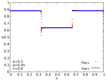
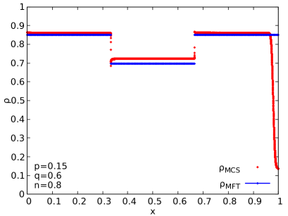
Figure 3: HD-HD-HD density plots: (top) $n=0.8,\,p=0.2,\,q=0.45$, (bottom) $n=0.8,\,p=0.15,\,q=0.6$. MFT (blue lines) and MCS (red points) results are shown. Good agreement between MFT and MCS results are observed.

MC-MC-MC phase:- In the MC phase, the density should be 1/2. This means in these putative MC phases, $J_{1}=J_{3}=1/4,\,J_{2}=q/4$. This immediately shows that there is no MC-MC-MC phase in the model, i.e., all the three segments cannot be simultaneously in the MC phases, as that would violate the current conservation condition (9).

III.1.2 Distinct phase solutions in MFT

We now consider the possibilities when each of $T_{1},T_{2}$ and $T_{3}$ can be in different, spatially uniform or even nonuniform stationary states separately. These are different phase states of the system. Let us first consider what happens when we start adding particles when the system is in its LD-LD-LD phase with a sufficiently low $n$. With addition of particles, $\rho_{1}=\rho_{3}<1/2$ and $\rho_{2}<1/2$ will rise, maintaining $J_{1}=J_{2}=J_{3}$ and $\rho_{1}=\rho_{3}<\rho_{2}<1/2$ (i.e., the LD-LD-LD phase). As $n$ keeps rising, the LD-LD-LD phase ultimately gives way to nonuniform phases. We argue below that this can happen in two distinct ways.

Point defect dominated steady states:- As $n$ rises, the LD-LD-LD phase is no longer the desired stationary state. This can be seen from the fact that the height $h$ of the local peak at $x=0$ in the LD-LD-LD phase continues to rise and the steady state current decreases as $p$ decreases. This cannot continue indefinitely. For instance, as argued in Refs. lebo ; niladri-tasep , in a periodic TASEP with just one point defect, as $n$ reaches a lower threshold

$$n=\frac{p}{1+p}$$ (18)

the point defect starts to have macroscopic effects in the form of a domain wall; see also Ref. erwin-defect . Physically, for a very low $n$, the system should be in its LD-LD-LD phase. The upon addition of particles, $n$ rises. As it rises, it eventually reaches a lower threshold, a macroscopically nonuniform steady state in the shape of a DW is formed. This threshold should obviously depend on the defect strengths. For a single point defect in an otherwise homogeneous ring (i.e., no extended defect, $q=1$) is as given in (18). This should however be different in the present model (marked $n_{cL}^{p}$ below; see below), when $q<1$. A DW, essentially a pile up of particles due to a bottleneck or a defect, should form behind the point defect, extending an HD phase up to a point $x_{w}$ and an LD phase from $x_{w}$ to 1. Hence it is first formed in $T_{1}$, as $n$ just exceeds $n_{cL}^{p}$ with the DW position $x_{w}$ being at $x=0$. As $n$ rises further above this lower threshold, the size of this pile or the DW increases by shifting its position $x_{w}$ (see below for a formal definition) along the ring, moving from $T_{1}$ first to $T_{2}$ and then to $T_{3}$, finally reaching $x=1$, at which point the DW ends at an threshold $n_{cU}^{p}$ of $n$ (see below), bringing the model to its HD-HD-HD phase. If $n$ is still increased, the system continues to remain in its HD-HD-HD phase till $n=1$ is reached, when the system gets fully filled. See sm1 for a related movie (Movie 1) that visually presents this picture. Below we provide a quantitative analysis that corroborates this intuitive picture.

First let us assume that the DW is located outside $T_{2}$, and is either in $T_{1}$ or in $T_{3}$, i.e., $0<x_{w}<\epsilon_{1}$, or $\epsilon_{1}+\epsilon_{2}<x_{w}<1$. In this case, $\rho_{2}$, the density of $T_{2}$, is spatially uniform. The DW being located either in $T_{1}$ or $T_{3}$, connects a low density segment with density $\rho_{\text{LD}}$ and a high density segment with density $\rho_{\text{HD}}$. We have

$$\rho_{\text{LD}}=\frac{p}{1+p},\,\rho_{\text{HD}}=\frac{1}{1+p}.$$ (19)

Using current conservation (7),

$$q\rho_{2}(1-\rho_{2})=\rho_{\text{LD}}(1-\rho_{\text{LD}})=\frac{p}{(1+p)^{2}}.$$ (20)

This is quadratic equation in $\rho_{2}$ that has two solutions

$$\rho_{2} = \frac{1}{2}\left[1\pm\{1-\frac{4p}{q(1+p)^{2}}\}^{1/2}\right]$$ (21)

$$= \rho_{2+}(>1/2),\,\rho_{2-}(<1/2).$$

Clearly, these solutions are physically acceptable, so long as $4p/[q(1+p)^{2}]<1$, or equivalently,

$$\frac{p}{(1+p)^{2}}<\frac{q}{4}.$$ (22)

We will come back to this condition below and re-interpret this in terms of the stationary currents.

Since the particles are hopping in the anticlockwise direction, subject to exclusion, any pile up of particles due to the point defect at $x=0$ will start just behind it, i.e., in $T_{1}$, and a DW is created. As more and more particles are added, the size of this “pile” of particles or the DW grows, and the DW position $x_{w}$ starts to move away from $x=0$. As a specific example, consider the case when the DW is inside $T_{1}$: $0\leq x_{w}\leq\epsilon_{1}$. Since the particles flow in the anticlockwise direction, and a DW should form behind a bottleneck (which in the present case is the point defect at $x=0$), we write

$$\rho_{1}(x) = \rho_{\text{HD}},\;\;0\leq x\leq x_{w},$$ (23)

$$= \rho_{\text{LD}},\;\;x_{w}\leq x\leq\epsilon_{1},$$

In this situation, we must have the entire $T_{2}$ to be its LD phase: $\rho_{2}(x)=\rho_{2-}$ for $\epsilon_{1}\leq x\leq\epsilon_{1}+\epsilon_{2}$. In addition, $T_{3}$ too should be in its LD phase, with $\rho_{3}=\rho_{\text{LD}}$. We can now apply PNC to determine $x_{w}$. We get

$$\rho_{\text{HD}}x_{w}+\rho_{\text{LD}}(\epsilon_{1}-x_{w})+\rho_{2-}\epsilon_{2}+\rho_{\text{LD}}(1-\epsilon_{1}-\epsilon_{2})=n.$$ (24)

Equation (24) gives $x_{w}$ as a function of $p,q$ and $n$. Simplifying (24), we obtain

$$x_{w}=\left(\frac{1+p}{1-p}\right)[n-\rho_{2-}\epsilon_{2}-\rho_{\text{LD}}(1-\epsilon_{2})].$$ (25)

Since a unique solution for $x_{w}$ can be obtained from (25), the DW has a fixed position and hence is an LDW. For $x_{w}>0$ but $<1$, there is an LDW in the bulk of $T_{1}$, making $\rho_{1}$ nonuniform, corresponding to the DW-LD-LD phase. See Fig. 4 for a plot showing an LDW in $T_{1}$ ($p=0.2000,n=0.35,q=0.65,L=9000,\epsilon_{1}=\epsilon_{2}=1/3$). Both MFT and MCS results are shown. If we set $x_{w}=0$, all of $T_{1},\,T_{2}$ and $T_{3}$ are in their LD phases, and is in fact the boundary between the LD-LD-LD phase and DW-LD-LD phase. We get

$$\frac{p}{1+p}(1-\epsilon_{2})+\frac{\epsilon_{2}}{2}\left[1-\sqrt{1-\frac{4p}{q(1+p)^{2}}}\;\right]=n=n_{cL}^{p},$$ (26)

a lower threshold on $n$, such that as $n$ exceeds $n_{cL}^{p}$ distinct phase solutions appear with the disappearance of the LD-LD-LD phase. As an example, if $T_{1},\,T_{2},\,T_{3}$ have the same size, i.e., if $\epsilon_{1}=\epsilon_{2}=1/3$, we get

$$\frac{2}{3}\frac{p}{1+p}+\frac{1}{6}\left[1-\sqrt{1-\frac{4p}{q(1+p)^{2}}}\right]=n_{cL}^{p}.$$ (27)

Furthermore, if we set $\epsilon_{2}=0$, i.e., effectively no extended defect, then $n_{cL}=p/(1+p)$, in agreement with Ref. niladri-tasep . On the other hand, at $x_{w}=\epsilon_{1}$ entire $T_{1}$ is in its HD phase; as $x_{w}$ exceeds $\epsilon_{1}$, $T_{2}$ is now its DW phase. Thus, $x_{w}=\epsilon_{1}$ gives HD-LD-LD phase and is the boundary between the DW-LD-LD phase and HD-DW-LD phase. We get

$$\frac{\epsilon_{1}}{1+p}+\frac{\epsilon_{2}}{2}\left[1-\sqrt{1-\frac{4p}{q(1+p)^{2}}}\,\right]$$

$$+\frac{p}{1+p}(1-\epsilon_{1}-\epsilon_{2})=n=n_{p1}.$$ (28)

In the particular case with $\epsilon_{1}=\epsilon_{2}=1/3$, we get

$$\frac{1}{3(1+p)}+\frac{1}{6}\left[1-\sqrt{1-\frac{4p}{q(1+p)^{2}}}\,\right]+\frac{p}{3(1+p)}=n=n_{p1}.$$ (29)

When the LDW is inside $T_{2}$, $T_{1}$ is in its HD phase, hence $\rho_{1}=\rho_{\text{HD}}$, and $T_{3}$ is in its LD phase, with $\rho_{3}=\rho_{\text{LD}}$. Further, since the LDW is located inside $T_{2}$, we must have $\rho_{2}=\rho_{+}$ for $\epsilon_{1}<x<x_{w}$; $\rho_{2}=\rho_{-}$ for $x_{w}<x<\epsilon_{1}+\epsilon_{2}$. Applying PNC we get

$$\rho_{\text{HD}}\epsilon_{1}+(x_{w}-\epsilon_{1})\rho_{2+}+(\epsilon_{1}+\epsilon_{2}-x_{w})\rho_{2-}+\rho_{\text{LD}}(1-\epsilon_{1}-\epsilon_{2})=n.$$ (30)

Solving (30), we get

$$x_{w} = \frac{1}{(\rho_{2+}-\rho_{2-})}\bigg{[}n+\rho_{2+}\epsilon_{1}-\rho_{\text{HD}}\epsilon_{1}$$ (31)

$$- (\epsilon_{1}+\epsilon_{2})\rho_{2-}-\rho_{\text{LD}}(1-\epsilon_{1}-\epsilon_{2})\bigg{]}$$

giving a unique position of the LDW in $T_{2}$. See Fig. 5 for an LDW in $T_{2}$ ($p=0.2,n=0.5,q=0.65,L=9000$). The overall density profile, consisting of HD phase in $T_{1}$ and LD phase in $T_{3}$, with an intervening LDW in $T_{2}$ takes the form of a step-like structure. This is specifically attributed to $T_{2}$ being an extended defect with a hopping rate $q<1$. Setting $x_{w}=\epsilon_{1}$ gives the boundary between the DW-LD-LD and HD-DW-LD phases (28). Next, if we set $x_{w}=\epsilon_{1}+\epsilon_{2}$ in (30), we get the HD-HD-LD phase, which gives the boundary between the HD-DW-LD and HD-HD-DW phases:

$$\frac{\epsilon_{1}}{1+p}+\frac{\epsilon_{2}}{2}\left[1+\sqrt{1-\frac{4p}{q(1+p)^{2}}}\;\right]$$ (32)

$$+ \frac{p}{1+p}(1-\epsilon_{1}-\epsilon_{2})=n=n_{p2}.$$

For the specific choice of equal-sized $T_{1},T_{2},T_{3}$, $\epsilon_{1}=\epsilon_{2}=1/3$, we get

$$\frac{1}{3}+\frac{1}{6}\left[1+\sqrt{1-\frac{4p}{q(1+p)^{2}}}\;\right]=n_{p2}.$$ (33)

Finally, consider an LDW in $T_{3}$. Thus, $\rho_{3}(x)=\rho_{\text{HD}},\;\epsilon_{1}+\epsilon_{2}<x<x_{w}$, $\rho_{3}(x)=\rho_{\text{LD}},\;x_{w}<x<1$. Further, $\rho_{1}(x)=\rho_{\text{HD}}$, $\rho_{2}(x)=\rho_{+}$, since both $T_{1}$ and $T_{2}$ are in their HD phases. Then applying PNC, we obtain

$$\frac{\epsilon_{1}}{1+p}+\frac{\epsilon_{2}}{2}\left[1+\sqrt{1-\frac{4p}{q(1+p)^{2}}}\;\right]$$

$$+(x_{w}-\epsilon_{1}-\epsilon_{2})\frac{1}{1+p}+\frac{(1-x_{w})p}{1+p}=n.$$ (34)

Solving, we find

$$x_{w}=\frac{1+p}{1-p}\left[n+\frac{\epsilon_{2}}{1+p}-\frac{p}{1+p}-\frac{\epsilon_{2}}{2}\left[1+\sqrt{1-\frac{4p}{q(1+p)^{2}}}\right]\right]$$ (35)

as the LDW position in $T_{3}$. See Fig. 6 for an LDW in $T_{3}$, where both MFT and MCS results are shown ($p=0.2,n=0.65,q=0.65,L=9000$). Setting $x_{w}=\epsilon_{1}+\epsilon_{2}$ gives HD-HD-LD phase, which exists on the boundary (32) between the HD-DW-LD and HD-HD-DW phases. On the other hand, if we set $x_{w}=1$, the LDW ends and the system is in its boundary between the HD-HD-DW phase and HD-HD-HD phase. We find

$$\frac{\epsilon_{1}}{1+p}+\frac{\epsilon_{2}}{2}\left[1+\sqrt{1-\frac{4p}{q(1+p)^{2}}}\;\right]$$ (36)

$$+ (1-\epsilon_{1}-\epsilon_{2})\frac{1}{1+p}=n=n_{cU}^{p},$$

an upper threshold on $n$, such that as $n$ exceeds $n_{cU}^{p}$, identical phase solutions reappear. For equal-sized $T_{1},T_{2},T_{3}$, we get

$$\frac{1}{3}+\frac{1}{6}\left[1+\sqrt{1-\frac{4p}{q(1+p)^{2}}}\;\right]=n_{cU}^{p}.$$ (37)

Further, if we set $\epsilon_{2}=0$, i.e., a vanishing extended defect, we get $n_{cU}^{p}=1/(1+p)$, as found in Ref. niladri-tasep .

Our MFT and MCS results on LDWs in $T_{1},\,T_{2},\,T_{3}$ are shown in Fig. 4, Fig. 5 and Fig. 6 respectively. We find reasonable agreement between our MFT and MCS results.

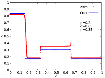
Figure 4: Plot of an LDW in $T_{1}$ in the point defect dominated regime with $p=0.2,n=0.35,q=0.65,L=9000,\epsilon_{1}=\epsilon_{2}=1/3$. MFT (blue lines) and MCS (red points) results are shown (see text).

Figure 5: Plot of an LDW in $T_{2}$ in the point defect dominated regime with $p=0.2,n=0.5,q=0.65,L=9000,\epsilon_{1}=\epsilon_{2}=1/3$. MFT (blue lines) and MCS (red points) results are shown (see text).

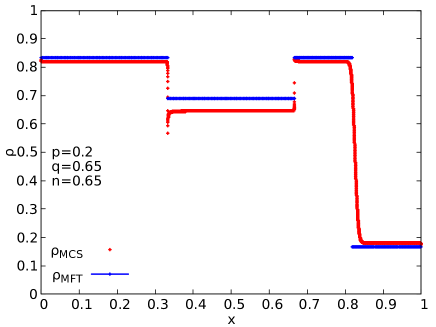
Figure 6: Plot of an LDW in $T_{3}$ in the point defect dominated regime with $p=0.2,n=0.65,q=0.65,L=9000,\epsilon_{1}=\epsilon_{2}=1/3$. MFT (blue lines) and MCS (red points) results are shown (see text).

Extended defect dominated steady states:- So far in the above, we have studied the situation where the point defect dominates by assuming that by adding particles $n$ reaches a threshold $n_{cL}^{p}$ above which the point defect enforces macroscopically nonuniform steady states. Alternatively, a rising $n$ can reach a different lower threshold, denoted $n_{cL}^{q}$ below, at which the extended defect enforces a DW. As $n$ rises, both $\rho_{1}=\rho_{3}$ and $\rho_{2}$ rise while being in their LD phases. Eventually, as $n$ reaches $n_{cL}^{q}$, $T_{2}$ reaches its MC phase with $\rho_{2}=1/2$ in the bulk, and $\rho_{1}=\rho_{3}<1/2$. As $n$ is further increased beyond $n_{c}^{q}$, a DW is formed in the system, just behind the bottleneck, which in the present case is $T_{2}$. This means a DW is first formed at $x=\epsilon_{1}+\epsilon_{2}$ in $T_{3}$ as soon as $n$ reaches $n_{c}^{q}$. As $n$ rises further, the DW starts moving along $T_{3}$, crossing over to $T_{1}$ at $x=0$, and then finally reaching $x=\epsilon_{1}$ at an upper density threshold $n_{cU}^{q}$, when the DW ends. Any further increase in $n$ will push the system to the HD-HD-HD phase. Thus, the DW never enters $T_{2}$, which remains in its MC phase. This is a fundamental difference with the LDW formed due to the point defect. This physical description is presented in a movie (Movie 2) in SM sm1 . Below we provide a quantitative analysis that corroborates this intuitive picture. We now work out the corresponding quantitative details that corroborates this intuitive picture.

Since $T_{2}$ is in its MC phase, we must have $\rho_{2}=1/2$ and $J_{2}=q/4$. Current conservation then yields

$$\rho(1-\rho)=\frac{q}{4},$$ (38)

where $\rho$ is $\rho_{1}$ or $\rho_{3}$. Solving,

$$\rho=\frac{1}{2}\left[1\pm\sqrt{1-{q}}\right]=\rho_{+}(>1/2),\rho_{-}(<1/2),$$ (39)

giving the densities of the high density and low density parts of the DW, which meet at $x_{w}$. As before, $x_{w}$ can be calculated by using PNC. Assume an LDW in $T_{3}$. This is the LD-MC-DW phase. Then PNC gives

$$\rho_{-}\epsilon_{1}+\frac{\epsilon_{2}}{2}+(1-x_{w})\rho_{-}+(x_{w}-\epsilon_{1}-\epsilon_{2})\rho_{+}=n.$$ (40)

Setting $x_{w}=\epsilon_{1}+\epsilon_{2}$ gives the condition for transition from the LD-LD-LD phase to LD-MC-DW phase, when the DW is due to the extended defect. We get

$$\epsilon_{1}\rho_{-}+\frac{\epsilon_{2}}{2}+(1-\epsilon_{1}-\epsilon_{2})\rho_{-}=n.$$ (41)

This is independent of $p$, but depends upon $q$ through the dependence of $\rho_{-}$ on $q$. Using (39), we find

$$(1-\epsilon_{2})\frac{1}{2}\left[1-\sqrt{1-{q}}\right]+\frac{\epsilon_{2}}{2}=n\equiv n_{cL}^{q},$$ (42)

defining a critical density $n_{c}^{q}$ above which an LDW due to the extended defect appears. For the particular case of $\epsilon_{1}=\epsilon_{2}=1/3$, we get

$$\frac{1}{3}\left[1-\sqrt{1-{q}}\right]+\frac{1}{6}=n_{cL}^{q}.$$ (43)

If we set $\epsilon_{2}=1/2$, i.e., the extended defect covers half of the ring, as case discussed in Refs. mustansir ; tirtha-niladri without any point defect (i.e., $p=1$), we get

$$\frac{1}{4}\left[1-\sqrt{1-{q}}\right]+\frac{1}{4}=n_{cL}^{q}.$$ (44)

If $x_{w}=1$, the system is at the boundary between its LD-MC-HD phase and DW-MC-HD phase, which is also the location of the (assumed subdominant in this Section) point defect. Now setting $x_{w}=1$ together with $\epsilon_{1}=1/4,\,\epsilon_{2}=1/2$ in (40), we find $n=1/2$, which is independent of $q$. We thus conclude that so long as the condition for an LDW due to the extended defect is satisfied, in the half-filled limit ($n=1/2$) with $\epsilon_{1}=1/4,\,\epsilon_{2}=1/2$, there is always an LDW at the location of the point defect, independent of the value of $q$ mustansir .

Now consider an LDW in $T_{1}$. In this case, $T_{3}$ is in the HD phase. PNC gives

$$x_{w}\rho_{+}+\frac{\epsilon_{2}}{2}+(1-\epsilon_{1}-\epsilon_{2})\rho_{+}+(\epsilon_{1}-x_{w})\rho_{-}=n.$$ (45)

Setting $x_{w}=\epsilon_{1}$ produces the boundary between the DW-MC-HD phase and HD-HD-HD phase:

$$(1-\epsilon_{2})\rho_{+}+\frac{\epsilon_{2}}{2}=n.$$ (46)

Substituting for $\rho_{+}$, we get

$$(1-\epsilon_{2})\frac{1}{2}\left[1+\sqrt{1-{q}}\right]+\frac{\epsilon_{2}}{2}=n\equiv n_{cU}^{q},$$ (47)

defining an upper threshold on $n$, such that for $n>n_{cU}^{q}$, identical phase solutions are predicted. In the special case of $\epsilon_{2}=1/3$, we get

$$\frac{1}{3}\left[1+\sqrt{1-q}\right]+\frac{1}{6}=n_{cU}^{q}.$$ (48)

Furthermore, in the case where $\epsilon_{2}=1/2$, we find

$$\frac{1}{4}\left[1+\sqrt{1-{q}}\right]+\frac{1}{4}=n_{cU}^{q},$$ (49)

see also Refs. mustansir ; tirtha-niladri . Our MFT and MCS results on LDWs in $T_{3}$ and $T_{1}$ are shown in Fig. 7 and Fig. 8 respectively. We find reasonable agreement between our MFT and MCS results.

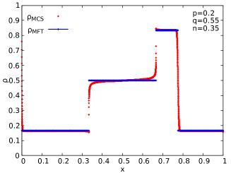
Figure 7: Plot of an LDW in $T_{3}$ in the extended defect dominated regime with $p=0.2,n=0.35,q=0.55,L=9000,\epsilon_{1}=\epsilon_{2}=1/3$. MFT (blue lines) and MCS (red points) results are shown (see text).

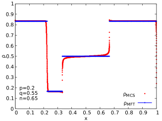
Figure 8: Plot of an LDW in $T_{1}$ in the extended defect dominated regime with $p=0.2,n=0.65,q=0.55,L=9000,\epsilon_{1}=\epsilon_{2}=1/3$. MFT (blue lines) and MCS (red points) results are shown (see text).

III.1.3 Minimum current principle and stationary state selections

We have discussed the possibilities of nonuniform steady steady states that can borne out of two distinct mechanisms - being controlled by the point defect or by the extended defect. We must then be able to specify which one will be observed for a given set of $p,q$. To do this end, we invoke a minimum current principle: among the possible steady state solutions, the one with the lowest stationary current should actually be observed.

To proceed further, we note that stationary current $J_{\text{PD}}$ corresponding to a domain wall due to the point defect is

$$J_{\text{PD}}=\frac{p}{(1+p)^{2}},$$ (50)

which depends only on $p$. Similarly, the stationary current $J_{\text{ED}}$ corresponding corresponding to a domain wall due to the extended defect is

$$J_{\text{ED}}=\frac{q}{4}.$$ (51)

Minimum current principle stipulates that when

$$J_{\text{PD}}<(>)J_{\text{ED}},$$ (52)

the nonuniform steady states are controlled by the point defect (extended defect).

When $J_{\text{PD}}=J_{\text{ED}}$, the two defects compete, as we illustrate below, a new kind of states - a pair of delocalised domain walls (DDW) emerges. The condition $J_{\text{PD}}=J_{\text{ED}}$ gives a unique relation between $p$ and $q$, which in the MFT is

$$\frac{p}{(1+p)^{2}}=\frac{q}{4},$$ (53)

- a line in the $p-q$ plane, on which the two defects compete and consequently a pair of DDWs emerge on this line in the $p-q$ plane. The numerical analogue of the line (53) has been measured in our MCS simulations by determining the emergence of a pair of DDWs for a particular $p,q$ pair. Both the MFT line (53) and the corresponding MCS results are shown in Fig. 9. We notice a small disagreement between the two, which we believe is due to the fluctuation effects ignored in the MFT.

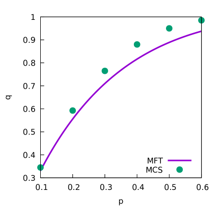
Figure 9: Plot of Eq. (53) in the $p-q$ plane (continuous line) and the corresponding MCS results (points) (see text).

III.2 Domain walls and the extended defect size

In the previous Section, we have discussed the minimum current principle in selecting the steady states. This analysis implicitly assumes selecting between an LDW due to the point defect and an LDW due to the extended defect. This holds when the density $n$ is above both the critical densities $n_{cL}^{p}$ and $n_{cL}^{q}$ for a domain wall due to the point defect and extended defect. However, $n_{cL}^{p}$ and $n_{cL}^{q}$ are in general unequal. Consider now a situation with $J_{\text{PD}}<J_{\text{ED}}$, i.e., the point defect dominates according to our previous analysis. Now consider

$$n_{cL}^{q}-n_{cL}^{p}=(1-\epsilon_{2})\frac{1}{2}\left[1+\sqrt{1-{q}}\right]+\frac{\epsilon_{2}}{2}$$ (54)

$$- \frac{p}{1+p}(1-\epsilon_{2})-\frac{\epsilon_{2}}{2}\left[1-\sqrt{1-\frac{4p}{q(1+p)^{2}}}\;\right].$$

Now consider the extreme limit of $\epsilon_{2}\rightarrow 1$, which means the size of $T_{2}$ is much greater than those of $T_{1}$ or $T_{3}$. In that limit,

$$n_{cL}^{q}-n_{cL}^{p}=\frac{1}{2}\sqrt{1-\frac{4p}{q(1+p)^{2}}}>0,$$ (55)

so long as $\frac{q}{4}-\frac{p}{(1+p)^{2}}>0$, which is equivalent to $J_{\text{PD}}<J_{\text{ED}}$, which in turn is what we have assumed. On the other hand, in the opposite limit of $\epsilon_{2}\rightarrow 0$, i.e., when $T_{1}$ or $T_{3}$ (or both) is much larger than $T_{2}$,

$$n_{cL}^{q}-n_{cL}^{p}<0$$ (56)

if

$$\frac{q}{4}<\frac{p}{(1+p)^{2}},$$ (57)

which contradicts the condition $J_{\text{PD}}<J_{\text{ED}}$. Therefore, $n_{cL}^{q}-n_{cL}^{p}>0$ necessarily for $\epsilon_{2}\rightarrow 0$, just as it is for $\epsilon_{2}\rightarrow 1$. Can $n_{cL}^{q}-n_{cL}^{p}$ be negative for intermediate values of $\epsilon_{2}$, i.e., for $0<\epsilon_{2}<1$? For this to happen, $n_{cL}^{q}-n_{cL}^{p}$ must flip sign for even number of times (at least twice) for intermediate values of $\epsilon_{2}$. Since (54) is linear in $\epsilon_{2}$, such a possibility is ruled out. Therefore, $n_{cL}^{q}-n_{cL}^{p}>0$ for all admissible values of $\epsilon_{2}$. This then means that with $J_{\text{PD}}<J_{\text{ED}}$, $n_{cL}^{q}-n_{cL}^{p}>0$ necessarily. Hence, as $n$ rises from a small value, it will first meet $n_{cL}^{p}$, creating an LDW due to the point defect.

III.3 Phase diagram for $\epsilon_{1}=1/3=\epsilon_{2}$

With $\epsilon_{1}=1/3=\epsilon_{2}$, the phases are determined by the mutual interplay between the defect strengths $p,\,q$ and the mean density $n$. A list of the phases is given in Table 1.

List of the phases
Phases	Types	Condition for existence	Dominant defect
LD-LD-LD	Identical	$n<n_{cL}^{p}$ with $J_{\text{PD}}<J_{\text{ED}}$ or $n<n_{cL}^{q}$ with $J_{\text{ED}}<J_{\text{PD}}$	None
HD-HD-HD	Identical	$n>n_{cU}^{p}$ with $J_{\text{PD}}<J_{\text{ED}}$ or $n>n_{cU}^{q}$ with $J_{\text{ED}}<J_{\text{PD}}$	None
DW-LD-LD	Distinct	$n_{p1}>n>n_{cL}^{p}$ with $J_{\text{PD}}<J_{\text{ED}}$	Point defect
HD-DW-LD	Distinct	$n_{p2}>n>n_{p1}$ with $J_{\text{PD}}<J_{\text{ED}}$	Point defect
HD-HD-DW	Distinct	$n_{cU}^{p}>n>n_{p2}^{p}$ with $J_{\text{PD}}<J_{\text{ED}}$	Point defect
LD-MC-DW	Distinct	$1/2>n>n_{cL}^{q}$ with $J_{\text{ED}}<J_{\text{PD}}$	Extended defect
DW-MC-HD	Distinct	$n_{cU}^{q}>n>1/2$ with $J_{\text{ED}}<J_{\text{PD}}$	Extended defect
DDW-MC-DDW	Distinct	$n_{cU}^{p}=n_{cU}^{q}>n>n_{cL}^{q}=n_{cL}^{p}$ with $J_{\text{ED}}=J_{\text{PD}}$	Point and extended defects equally dominant

Table 1: List of the phases on the segments $T_{1},T_{2},T_{3}$.

In this Section, we present a phase diagram of the model in the $p-q-n$ space. To proceed, we first list the phase boundaries between the different phases.

(i) Transition between the LD-LD-LD to DW-LD-LD phases (controlled by the point defect):

$$\frac{2p}{1+p}+\frac{1}{2}\left[1-\sqrt{1-\frac{4p}{q(1+p)^{2}}}\;\right]=3n.$$ (58)

(ii) Transition between the HD-HD-DW to HD-HD-HD phases (controlled by the point defect):

$$\frac{2}{1+p}+\frac{1}{2}\left[1+\sqrt{1-\frac{4p}{q(1+p)^{2}}}\;\right]=3n.$$ (59)

(iii) Transition between LD-LD-LD to LD-MC-DW phases (controlled by the extended defect):

$$\sqrt{1-{q}}=3(\frac{1}{2}-n).$$ (60)

This is independent of $p$.

(iv) Transition between HD-HD-HD and DW-MC-HD phases (controlled by the extended defect):

$$-\sqrt{1-{q}}=3(\frac{1}{2}-n).$$ (61)

Again, this is independent of $p$. The mean-field phase diagram in the $p-q-n$ space is shown in Fig.10

Figure 10: Mean-field phase diagram of the model in the $p-q-n$ space showing the phases in the model. HD and DW (with one LDW) phases are marked. LD phase that lies below the DW phase in the figure is not visible. Points on the gray curved plane lying as a divider of the DW phase have $J_{\text{PD}}=J_{\text{ED}}$ [see Eq. (53)] satisfied and hence have a pair of DDWs fully or partially covering $T_{1}$ and $T_{3}$. In the DW phase region, on the right of this curved surface (i.e., with $J_{\text{PD}}<J_{\text{ED}}$, there is an LDW due to the point defect in either $T_{1},T_{2}$ or $T_{3}$; on the left of this plane (i.e., with $J_{\text{ED}}<J_{\text{PD}}$, one has an LDW due to the extended defect in $T_{1}$ or $T_{3}$ and correspondingly an MC phase in $T_{2}$. In the HD (LD) phase region, one has HD-HD-HD (LD-LD-LD) phase in $T_{1},T_{2},T_{3}$ (see text).

III.4 Jump in the LDW position across $J_{\text{PD}}=J_{\text{ED}}$

We focus on the case $\epsilon_{1}=1/3=\epsilon_{2}$. Consider the LD-MC-HD phase that comes with an LDW at $x_{w}=0$, which is also the location of the point defect. This LDW is due to the extended defect. Using (41),

$$\frac{1}{6}\left[1-\sqrt{1-{q}}\;\right]+\frac{1}{6}+\frac{1}{6}\left[1+\sqrt{1-{q}}\;\right]=n,$$ (62)

giving $n=1/2$, independent of $p$ and $q$. Thus, so long as the extended defect “dominates”, i.e., $J_{\text{ED}}<J_{\text{PD}}$ is satisfied, there is always an LDW at $x_{w}=0$ with $n=1/2$.

What happens in the other limit, i.e., $J_{\text{ED}}>J_{\text{PD}}$ with $n=1/2$? In this case, the point defect controls the steady state. Now, if there is an LDW in $T_{1}$, then

$$\frac{1-p}{1+p}x_{w}+\frac{2p}{3(1+p)}+\frac{1}{6}\left[1-\{1-\frac{4p}{q(1+p)^{2}}\}^{1/2}\right]=n.$$ (63)

Since the LDW is assumed to be confined in $T_{1}$, max$(x_{w})$=1/3. Since $n$ rises with $x_{w}$ monotonically, we have

$$\text{max}({n})=\frac{1}{3}+\frac{1}{6}\left[1-\{1-\frac{4p}{q(1+p)^{2}}\}^{1/2}\right]<\frac{1}{2}.$$ (64)

On the other hand, if there is an LDW in $T_{3}$,

$$\frac{1}{3(1+P)}+\frac{1}{6}\left[1-\{1-\frac{4p}{q(1+p)^{2}}\}^{1/2}\right]$$ (65)

$$+ (x_{w}-\frac{2}{3})\frac{1}{1+P}+(1-x_{w})\frac{P}{1+P}=n.$$

Now, min$(n)$ is when $x_{w}=2/3$. This gives

$$\text{min}(n)=\frac{1}{3}+\frac{1}{6}\left[1+\{1-\frac{4p}{q(1+p)^{2}}\}^{1/2}\right]>\frac{1}{2}.$$ (66)

Therefore if $n=1/2$, the LDW cannot be in $T_{1}$ or $T_{3}$; it must be somewhere in $T_{2}$. Now, assuming an LDW in $T_{2}$,

$$\frac{1}{2}-(x_{w}-\frac{1}{2})\sqrt{1-\frac{4p}{q(1+p)^{2}}}=n.$$ (67)

Thus, if $n=1/2$, $x_{w}=1/2$, i.e., the LDW, now formed due to the point defect, appears at the mid point of the extended defect or $T_{2}$.

We thus note that with $n=1/2$ the positions $x_{w}$ of the LDW are at diametrically opposite points $x_{w}=0$ and $x_{w}=1/2$, when controlled by the point defect and extended defect respectively. Let and $n=1/2$ and $p_{c},\,q_{c}$ satisfy $J_{\text{PD}}=J_{\text{ED}}$. Then if $p=p_{c}-\delta_{1},\,q=q_{c}+\delta_{2},\,\delta_{1},\,\delta_{2}>0$ (but $\delta_{1},\,\delta_{2}$ are very small) $J_{\text{PD}}<J_{\text{ED}}$, we have an LDW at $x_{w}=1/2$ due to the point defect. On the other hand, if $\delta_{1},\,\delta_{2}<0$, $J_{\text{ED}}<J_{\text{PD}}$ and hence an LDW at $x_{w}=0$. Thus, as one moves ${\cal O}(\delta),\,\delta=\delta_{1},\,\delta_{2}$ being vanishingly small, the DW position changes by an ${\cal O}(1)$ amount - from $x_{w}=0$ to $x_{w}=1/2$. Thus, the domain wall position as a function of $\delta_{1},\delta_{2}$ (or $p,q$) shows a jump across the line $J_{\text{PD}}=J_{\text{LD}}$. This may be described in a more quantitative way. Let $\delta\equiv 2\sqrt{\delta_{1}^{2}+\delta_{2}^{2}}$ be the “distance” between the two points $(p=p_{c}-\delta_{1},\,q=q_{c}+\delta_{2})$ and $p=p_{c}+\delta_{1},\,q=q_{c}-\delta_{2}$ in the $p-q$ plane. Then, $dx_{w}/d\delta$ diverges for small $\delta$. Such divergences can occur only when the two points in the $p-q$ plane lie on the two sides of the line determined by the condition $J_{\text{PD}}=J_{\text{ED}}$.

III.5 Delocalised DW

Let us now consider the steady states on the critical line in the $p-q$ plane given by $J_{\text{PD}}=J_{\text{ED}}$. On this line, there should be a domain wall due to the point defect, so long as $n>n_{cL}^{p}$ for a particular value of $p$. Let us assume that it is at $x=x_{w}^{\text{PD}}$. On the other hand, there should be a domain wall, say at $x=x_{w}^{\text{ED}}$, due to the extended defect, provided $n>n_{cL}^{q}$. Thus, a complete description of the stationary density profiles require enumeration of both $x_{w}^{\text{PD}}$ and $x_{w}^{\text{ED}}$. However, with just one condition, viz., the PNC at hand, both $x_{w}^{\text{PD}}$ and $x_{w}^{\text{ED}}$ cannot be uniquely determined. Rather only a linear relation between the two is obtained. This then means any pair of ($x_{w}^{\text{PD}}$, $x_{w}^{\text{ED}}$) satisfying PNC is a valid solution, giving positions of the two LDW’s. Since an LDW due to the extended defect must be confined to $T_{1}$ and $T_{3}$ only, other LDW due to the point defect must also be confined to the same (even though an LDW due to an isolated point defect with $J_{\text{PD}}<J_{\text{ED}}$ can also be in $T_{2}$). Thus, each of ($x_{w}^{\text{PD}}$, $x_{w}^{\text{ED}}$) must be confined to $T_{1}$ or $T_{2}$ only. The inherent stochasticity of the dynamics implies all such valid ($x_{w}^{\text{PD}}$, $x_{w}^{\text{ED}}$) pairs satisfying PNC will be visited over time. This further means long-time averages of the densities take the form of inclined straight lines. See sm1 for a related movie (Movie 3) that visually presents this picture, showing a pair of DDWs. Below we provide a quantitative analysis that corroborates this intuitive picture.

Consider an specific example with $n_{cL}^{p},\,n_{cL}^{q}<n<1/2$ together with $J_{\text{ED}}=J_{\text{PD}}$. We then expect a DW behind the point defect in $T_{1}$ at, say, $x_{w}^{\text{PD}}$, and another behind the extended defect in $T_{3}$ at, say, $x_{w}^{\text{ED}}$. The condition $J_{\text{ED}}=J_{\text{PD}}$ ensures that both the DWs must have the same height given by $(1-p)/(1+p)$, with $\rho_{\text{HD}}=1/(1+p),\,\rho_{\text{LD}}=p/(1+p),\,\rho_{2}=1/2$. Applying PNC,

$$\rho_{\text{HD}}x_{w}^{\text{PD}}+\rho_{\text{LD}}(\epsilon_{1}-x_{w}^{\text{PD}})+\frac{\epsilon_{2}}{2}+\frac{x_{w}^{\text{ED}}-\epsilon_{1}-\epsilon_{2}}{1+p}$$

$$+(1-x_{w}^{\text{ED}})\frac{p}{1+p}=n.$$ (68)

Clearly, (68) gives only a linear relations connecting $x_{w}^{\text{PD}}$ and $x_{w}^{\text{ED}}$, and not each of the positions separately. As a result, a pair of DDWs is observed. MFT cannot predict the profiles of the DDWs, as it neglects fluctuations. However, we can employ arguments based on symmetry to construct the DDW profiles. First consider the special case $\epsilon_{1}=1/3=\epsilon_{2}$. Equation (68) simplifies to

$$\rho_{\text{HD}}x_{w}^{\text{PD}}+\rho_{\text{LD}}(\frac{1}{3}-x_{w}^{\text{PD}})+\frac{1}{6}+\frac{x_{w}^{\text{ED}}-2/3}{1+p}$$

$$+(1-x_{w}^{\text{ED}})\frac{p}{1+p}=n.$$ (69)

Statistically, with equal-sized segments $T_{1},T_{2},T_{3}$ both the DDWs must symmetric, i.e., the configuration of the long time averaged envelop of the DDW in $T_{1}$ must be same as the configuration of the long time averaged envelop of the DDW in $T_{3}$. To know the midpoint for each of them, we hypothetically replace each of them by an LDW of height $(1-p)/(1+p)$, connecting $\rho_{\text{HD}}=1/(1+p)$ and $\rho_{\text{LD}}=p/(1+p)$. Such (hypothetical) replacements evidently satisfy the PNC. Symmetry of the problem dictates that if $x_{0}$ is the position of the LDW in $T_{1}$, the corresponding LDW in $T_{3}$ must be located at $x_{0}+2/3$. This ensures that each of the LDW has HD (or LD) phase parts with the same length, as necessary from the symmetry considerations. Now in terms of these two LDWs, the PNC reads

$$2x_{0}\frac{1}{1+p}+2(\frac{1}{3}-x_{0})\frac{p}{1+p}+\frac{1}{6}=n.$$ (70)

This gives

$$2x_{0}\frac{1-p}{1+p}=n-\frac{1}{6}-\frac{2}{3}\left(\frac{p}{1+p}\right).$$ (71)

Clearly, if $n=1/2$, $x_{0}=1/6$, which means the midpoint of the LDW is at the midpoint of $T_{1}$ or $T_{3}$. If $n<1/2$, $x_{0}<1/6$, whereas $n>1/2$, $x_{0}>1/6$. Our MCS results on DDWs in $T_{1},\,T_{3}$ are shown in Fig. 11, Fig. 12 and Fig. 13 respectively. The analytically obtained DDW profiles are also shown.

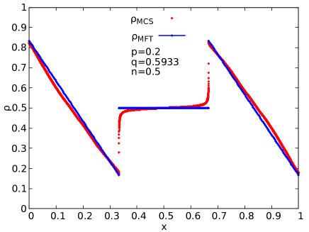
Figure 11: Plot of a pair of DDWs in $T_{1}$ and $T_{3}$ with $n=0.5,\,p=0.2,\,q=0.5933,\,L=9000,\,\epsilon_{1}=\epsilon_{2}=1/3$. Each DDW spans the entire respective segments $T_{1}$ or $T_{3}$ from our MCS results (red points). The analytically obtained DDW profiles (blue lines) are also shown (see text).

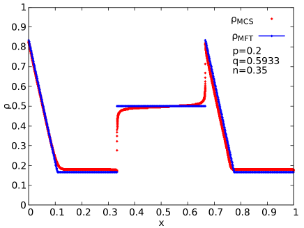
Figure 12: Plot of a pair of DDWs in $T_{1}$ and $T_{3}$ with $n=0.35,\,p=0.2,\,q=0.5933,\,L=9000,\,\epsilon_{1}=\epsilon_{2}=1/3$. Each DDW spans the respective segments $T_{1}$ or $T_{3}$ partially with the remaining part being in the LD phase from our MCS results (red points). The analytically obtained DDW profiles (blue lines) are also shown (see text).

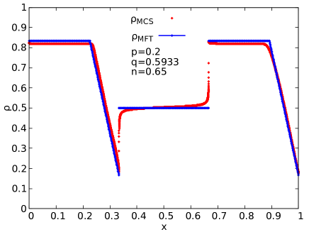
Figure 13: Plot of a pair of DDWs in $T_{1}$ and $T_{3}$ with $n=0.65,\,p=0.2,\,q=0.5933,\,L=9000,\,\epsilon_{1}=\epsilon_{2}=1/3$. Each DDW spans the respective segments $T_{1}$ or $T_{3}$ partially with the remaining part being in the HD phase from our MCS results (red points). The analytically obtained DDW profiles (blue lines) are also shown (see text).

III.6 MCS algorithm

In our stochastic simulations, we have used sequential updating of the sites of the TASEP with a periodic boundary condition. We perform stochastic simulations of the model subject to the update rules (a)-(d) described above in Sec. II by using a random sequential updating scheme rand . In each iteration, we choose a site in the TASEP random-sequentially for updating. The stationary densities are calculated by temporal averaging, once the system reaches steady states. This naturally produces time-averaged, space-dependent, steady state density profiles, which are then used to calculate the phase diagram.

IV Summary and outlook

We have thus studied a periodic TASEP with a point and an extended defects, of strengths $p$ and $q$. We have used a combination of MFT and extensive MCS studies to systematically explore how the interplay between the trio of the two defect strengths and mean number density ultimately result into the stationary density profiles. The MFT and MCS studies results agree reasonably well. We show that while for small (closed to zero) and high (closed to unity) mean densities, the TASEP should be in either the LD or HD phases. For mean densities in intermediate ranges, i.e., when it is neither too high nor too low, domain walls are observed. In general there is a single domain wall which is pinned to a particular point in the TASEP lane, i.e., an LDW is formed, with its height and location being functions of either $p$ or $q$ and $n$, the mean density. There is a fundamental distinction between an LDW formed by a point defect, and the one formed by an extended defect: While the former can be found anywhere in the ring including inside the extended defect segment, with its position being continuously tuned by $n$, the mean density, the latter must always be outside of the extended defect segment. We have further shown that for intermediate values of $n$, controlled by $p$ and $q$, there can a pair of DDWs instead one LDW, when $p$ and $q$ maintains a specific relationship. These DDWs must remain outside the extended defect segment. These DDWs can be partial or full, i.e., they can jointly cover only a part of the remaining part of the ring, or the whole of the remaining ring (i.e., excluding the extended defect). We invoke a minimum current principle to explain the LDW either due to a point defect or an extended defect, and also the pair of DDWs. We have argued that the latter appear when certain conditions on the steady state currents controlled by of the point defect or the extended defect hold.

In the present work, we have focussed on a periodic TASEP with just one point defect and one uniform extended defect as a prototype system to explore the consequence of competitions between defects of different types. In possible natural realisations of the system, there can be more than one point and extended defects of different strengths. Furthermore, these extended defect segments themselves need not be uniform, i.e., can have spatially varying hopping in the segment. A TASEP with open boundaries or in a ring geometry having spatially continuously varying hopping rates can already give surprisingly nontrivial stationary densities atri ; tirtha-qkpz . Now adding competition between such spatially nonuniform hopping rates with point defects are expected to introduce complex density profiles and phase diagrams. Yet another direction of research that follows from our work would be introduce time-dependent defects, where the either strength or location or both can be changing. Thus the defects become annealed as opposed to being quenched in the present study. Such annealed defects can introduce further elements of competition due to the possible fast to slow defect dynamics relative to the TASEP hopping rates. It would also be interesting to study the effects of coupling an inhomogeneous TASEP with diffusive processes on the steady states atri2 . We hope our work here will stimulate further research along these directions.

V Acknowledgement

S.M. thanks SERB (DST), India for partial financial support through the CRG scheme [file: CRG/2021/001875].

References

- (1) C. T. MacDonald, J. H. Gibbs and Allen C. Pipkin, Kinetics of biopolymerization on nucleic acid templates, Biopolymers 6, 1 (1968).
- (2) J. Kärger and D. Ruthven, Diffusion in Zeolites and Other Microporous Solids (New York: Wiley)
- (3) D. Chowdhury, L. Santen, and A. Schadschneider, Statistical physics of vehicular traffic and some related systems, Phys. Rep. 329, 199 (2000).
- (4) J. Krug, Boundary-induced phase transitions in driven diffusive systems, Phys. Rev. Lett. 67, 1882 (1991).
- (5) B. Derrida, M. R. Evans, V. Hakim, and V. Pasquier, Exact solution of a 1d asymmetric exclusion model using a matrix formulation,” J. Phys. A: Math. Gen. 26, 1493 (1993).
- (6) B. Schmittmann and R. Zia, in Phase Transitions and Critical Phenomena, edited by C. Domb and J. L. Lebowitz (Academic, London, 1995).
- (7) T. Chou, K. Mallick, and R. K. P. Zia, Non-equilibrium statistical mechanics: from a paradigmatic model to biological transport, Rep. Prog. Phys. 74, 116601 (2011).
- (8) J. J. Dong, B. Schmittmann, and R. K. P. Zia, Towards a Model for Protein Production Rates, J. Stat. Phys. 128, 21 (2007).
- (9) P. Greulich and A. Schadschneider, Phase diagram and edge effects in the ASEP with bottlenecks, Physica A 387, 1972 (2008).
- (10) R. K. P. Zia, J. J. Dong, and B. Schmittmann, Modeling Translation in Protein Synthesis with TASEP: A Tutorial and Recent Developments, J. Stat. Phys. 144, 405 (2011).
- (11) J. S. Nossan, Disordered exclusion process revisited: some exact results in the low-current regime, J. Phys. A: Math. Theor. 46, 315001 (2013).
- (12) J. Schmidt, V. Popkov, and A. Schadschneider, Defect-induced phase transition in the asymmetric simple exclusion process, Europhys. Lett. 110, 20008 (2015).
- (13) S. A. Janowsky and J. L. Lebowitz, Finite-size effects and shock fluctuations in the asymmetric simple-exclusion process, Phys. Rev. A 45, 618 (1992).
- (14) N. Sarkar and A. Basu, Nonequilibrium steady states in asymmetric exclusion processes on a ring with bottlenecks, Phys. Rev. E 90, 022109 (2014).
- (15) G. Tripathy and M. Barma, Driven lattice gases with quenched disorder: Exact results and different macroscopic regimes, Phys. Rev. E 58, 1911 (1998).
- (16) T. Banerjee, N. Sarkar and A. Basu, Generic nonequilibrium steady states in an exclusion process on an inhomogeneous ring, J. Stat. Mech. J. Stat. Mech. P01024 (2015).
- (17) T. Chou, Ribosome Recycling, Diffusion, and mRNA Loop Formation in Translational Regulation, Biophys. J. 85, 755 (2003).
- (18) S. E. Wells, E. Hillner, R. D. Vale and A. B. Sachs, Circularization of mRNA by Eukaryotic Translation Initiation Factors, Mol. Cell 2, 135 (1998).
- (19) G. S. Kopeina et al, Step-wise formation of eukaryotic double-row polyribosomes and circular translation of polysomal mRNA, Nucleic Acids Res. 36, 2476 (2008).
- (20) Robinson M et al, Codon usage can affect efficiency of translation of genes in Escherichia coli, Nucleic Acids Res. 12, 6663 (1984).
- (21) M. A. Sorensen, C. G. Kurland and S. Pedersen, Codon usage determines translation rate in Escherichia coli, J. Mol. Biol. 207, 365 (1989).
- (22) D. A. Phoenix and E. Korotkov, Evidence of rare codon clusters within Escherichia coli coding regions, FEMS Microbiol. Lett. 155, 63 (1997).
- (23) R A Blythe and M R Evans, Nonequilibrium steady states of matrix-product form: a solver’s guide, J. Phys. A 40, R333 (2007).
- (24) H. Hinsch and E. Frey, Bulk-driven nonequilibrium phase transitions in a mesoscopic ring, Phys. Rev. Lett. 97, 095701 (2006).
- (25) P. Roy, A. K. Chandra and A. Basu, Pinned or moving: States of a single shock in a ring, Phys. Rev. E 102, 012105 (2020).
- (26) A. Haldar, P. Roy and A. Basu, Asymmetric exclusion processes with fixed resources: Reservoir crowding and steady states, Phys. Rev. E 104, 034106 (2021).
- (27) P. Pierobon, M. Mobilia, R. Kouyos and E. Frey, Bottleneck-induced transitions in a minimal model for intracellular transport, Phys. Rev. E 74, 031906 (2006).
- (28) Supplemental Material movie
- (29) N. Rajewsky, L. Santen, A. Schadschneider and M. Schreckenberg, The asymmetric exclusion process: Comparison of update procedures, Journal of Statistical Physics 92, 151 (1998).
- (30) A. Goswami, M. Chatterjee and S. Mukherjee, Steady states and phase transitions in heterogeneous asymmetric exclusion processes, J. Stat. Mech. 123209 (2022).
- (31) T. Banerjee and A. Basu, Smooth or shock: Universality in closed inhomogeneous driven single file motions, Phys. Rev. Research 2, 013025 (2020).
- (32) A. Goswami, U. Dey and S. Mukherjee, Nonequilibrium steady states in coupled asymmetric and symmetric exclusion processes, Phys. Rev. E 108, 054122 (2023).