A Physics-Informed Deep Learning Description of Knudsen Layer Reactivity Reduction
Abstract
A physics-informed neural network (PINN) is used to evaluate the fast ion distribution in the hot spot of an inertial confinement fusion target. The employment of customized input and output layers to the neural network are shown to enable a PINN to learn the parametric solution to the Vlasov-Fokker-Planck equation in the absence of any synthetic or experimental data. While the offline training of the PINN is computationally intensive, online deployment is rapid, thus enabling an efficient surrogate of the fast ion tail across a broad range of hot spot conditions. As an explicit demonstration of the approach, the specific problem of Knudsen layer fusion yield reduction is treated. Here, predictions from the Vlasov-Fokker-Planck PINN are used to provide a non-perturbative solution of the fast ion tail in the vicinity of the hot spot thus allowing the spatial profile of the fusion reactivity to be evaluated for a range of collisionalities and hot spot conditions. Excellent agreement is found between the predictions of the Vlasov-Fokker-Planck PINN and results from traditional numerical solvers with respect to both the energy and spatial distribution of fast ions and the fusion reactivity profile demonstrating that the Vlasov-Fokker-Planck PINN provides an accurate and efficient means of determining the impact of Knudsen layer yield reduction across a broad range of plasma conditions.
I Introduction
Inertial confinement fusion (ICF) experiments generate plasmas that encompass an exceptionally broad range of densities and temperatures. This broad range of plasma conditions creates a challenge with regard to selecting the level of physics fidelity required for accurately describing an ICF implosion. In particular, while radiation-hydrodynamic codes have emerged as the backbone to integrated simulations of ICF capsules Clark et al. (2011); Johnson et al. (2020), such a framework is based on perturbative closures that are only valid for asymptotically small values of the Knudsen number , where is the particle’s mean-free-path and is the smallest gradient length scale. While the limit is well satisfied across a range of ICF conditions, this limit is strongly violated in low density exploding pusher experiments Rosenberg et al. (2014); Rinderknecht et al. (2015), and due to the strong temperature dependence of the Knudsen number (), becomes increasingly suspect for burning plasmas capable of achieving high ion and electron temperatures Hartouni et al. (2023).
The presence of low to modest levels of collisionality allow for strong deviations from a local Maxwellian distribution to develop that cannot be treated by perturbative closures Chapman et al. (1990); Braginskii (1958). Such deviations of an ion or electron distribution from a local Maxwellian impact closure quantities such as the heat flux Spitzer Jr and Härm (1953); Epperlein and Short (1991); Schurtz et al. (2000); Chapman et al. (2021); Miniati and Gregori (2022), the magnitude and spatial profile of the fusion reactivity Henderson (1974); Petschek and Henderson (1979); Molvig et al. (2012); McDevitt et al. (2014a); Kagan et al. (2015), atomic physics rates Garland et al. (2022), and thus can strongly impact the trajectory of an ICF implosion Rinderknecht et al. (2018). In addition, sufficiently strongly deviations from a Maxwellian impact diagnostics based on neutron Frenje (2020); Crilly et al. (2022) or hard X-ray spectra Kagan et al. (2019). In this paper we describe how physics-informed machine learning methods enable the development of an efficient surrogate model for the tail ion distribution to be rapidly inferred. Such an approach offers a complement to traditional numerical solvers focusing on the solution to the Vlasov-Fokker-Planck equation Larroche (2012); Taitano et al. (2015). Here, rather than relying on data, this approach seeks to embed physical constraints into the training of a neural network Karniadakis et al. (2021). In so doing, the quantity of data needed to train the neural network (NN) can be sharply reduced, or even eliminated.
As an initial study, we demonstrate the ability of this approach to provide a comprehensive description of Knudsen layer reactivity reduction in the hot spot of an ICF target. In particular, a physics-informed neural network (PINN) is used to solve the time dependent Vlasov-Fokker-Planck (VFP) equation for a geometry with one spatial dimension and two velocity space dimensions (1D-2V) in the absence of any data. It is shown that the VFP PINN is able to learn the parametric dependence of solutions to the Vlasov-Fokker-Planck equation, thus enabling a fast surrogate model of plasma kinetic effects.
The remainder of this paper is organized as follows. Section II provides a brief description of physics-informed neural networks, with an emphasis on how they may be used to learn the solution space of parametric PDEs Sun et al. (2020). An overview of the system of equations solved is given in Sec. III, along with a description of how customized input and output layers are included for treating the specific problem of the fast ion distribution in the vicinity of a plasma hot spot. Section IV describes the fast ion solution predicted by the VFP PINN. The fusion yield of an ICF hot spot is described in Sec. V, along with a comprehensive description of how hot spot parameters impact Knudsen layer yield reduction. Conclusions and a brief discussion are given in Sec. VI.
II Physics-Constrained Deep Learning
A primary aim of this paper is the development of a PINN customized to treat the Vlasov-Fokker-Planck equation. Before doing so, it will be useful to briefly review fundamental aspects of the PINN framework, which has emerged as a prominent example of physics-informed machine learning methods Lagaris et al. (1998); Karpatne et al. (2017); Karniadakis et al. (2021); Lusch et al. (2018); Wang et al. (2020). The present discussion will only focus on the essential concepts, where the interested reader is referred to Ref. Karniadakis et al. (2021) and references therein for a more detailed discussion. Here, the underlying strategy is to impose physical constraints into the training of a neural network. This can be accomplished either via the use of customized layers in the neural network (i.e. as hard constraints), or via the addition of physical constraints into the loss function (soft constraints). A PINN in its simplest form is focused on the latter strategy, with the loss expressed as Raissi et al. (2019):
| Loss | ||||
| (1) |
where represents the field being solved for (the ion distribution in the present paper), are phase space coordinates (energy, pitch and a spatial coordinate), is time, represents parameters of the physical system (Knudsen number, for example), and is the residual of the PDE. The second and third terms on the right hand side are to set boundary and initial conditions, respectively. An additional loss term containing any available data can be added to the loss in Eq. (1), though no data will be used in the present study. Our motivation will instead be to demonstrate the ability of PINNs to accurately learn solutions to the Vlasov-Fokker-Planck equation across a broad range of parameters in the zero data limit. As described in Sec. III.2 below, the use of a vanilla PINN such as Eq. (1) will fail to accurately evaluate the ion distribution at high energies. A primary motivation of the present work will thus be to develop a tailored PINN, with a loss function and custom input and output layers that ensure physical constraints and symmetries of the system are exactly satisfied.
III Model Equations
III.1 Physics Model
For modest Knudsen numbers, ions in the bulk plasma will be nearly Maxwellian, and will thus be well approximated by collisional closures based on perturbative Chapman-Enskog expansions Chapman et al. (1990). Due to the mean-free-path of an ion scaling with the square of the ion’s energy, however, we anticipate strong deviations from a Maxwellian distribution at high energy. An accurate description of such deviations can be achieved by utilizing a test-particle collision operator, whereby the fast ion population is evolved under the assumption that collisions between the tail and Maxwellian bulk are dominant compared to tail-tail collisions Tang et al. (2014a). Under such an assumption, the fast ion population can be described by a test-particle collision operator, resulting in the Vlasov-Fokker-Planck equation reducing to McDevitt et al. (2014b):
| (2) |
where the collisional coefficients are defined by:
| (3a) | |||
| (3b) | |||
| (3c) | |||
| (3d) | |||
| (3e) |
with the normalizations
Here, is the hot spot temperature, is the density at the center of the hot spot, , we have assumed a slab geometry with one spatial dimension , is half the system size, is the ion kinetic energy, and is the pitch. For non-thermal ions satisfying , the dimensionless collision frequencies for a DT plasma are given by:
| (4) | |||
| (5) |
where is the mean free path of a thermal ion. The collisional dependence can be described by the Knudsen number defined by:
| (6) |
where is the Coulomb logarithm, taken as a constant in the present study for simplicity. We have also defined the quantity , which defines the energy scale above which ion slowing down by electrons becomes dominant, i.e.
| (7) |
While in the hot spot, noting that decreases with temperature, this term will impact ion slowing down in the neighboring cold plasma.
Our aim will be to utilize a PINN to evaluate the ion distribution in an idealized hot spot, where for definiteness we adopt an analogous slab geometry and profiles as adopted in Ref. McDevitt et al. (2014b). In particular, we will assume an isobaric equilibrium with density and temperature profiles of the form
where , , and for simplicity we have assumed each particle species to have the same temperature. For all cases treated in this work we will take . The electric field will be evaluated from the electron equation of motion, which can be approximated by:
| (8) |
Here, describes electron-ion momentum exchange, and we have neglected the electron inertia and viscosity terms. For an electron-proton plasma, the thermal force in the momentum exchange term can be written as , with Braginskii and Leontovich (1965). After normalization, the electric field can then be expressed as:
| (9) |
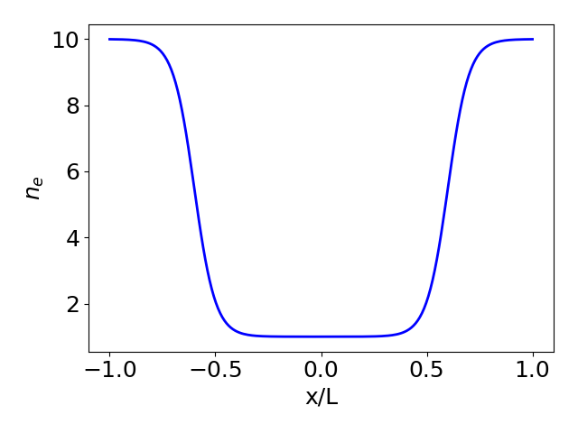
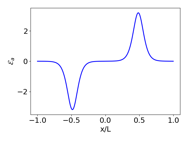
where since we are considering an isobaric equilibrium, with no equilibrium ion or electron flow, only the thermal force contributes to the electric field. The sign of this electric field is such that it accelerates ions away from the hot spot, thus enhancing fast ion losses. The assumed density and electric field profiles are shown in Fig. 1. For the remainder of this paper we will drop overbars of normalized quantities for notational simplicity unless explicitly indicated.
To complete the description of the problem setup we will need to introduce initial and boundary conditions. With regard to the boundary conditions, we will match the ion distribution to a Maxwellian at the low energy boundary, and take its value to be a small value at the high energy boundary. While no rigorous boundary condition is available at the high energy boundary, taking the distribution to a small value was shown in Ref. McDevitt et al. (2014b) to have a minimal impact on the solution of the fast ion distribution throughout the energies that strongly impact the fusion reactivity. The specific value of the distribution at the high energy boundary will be taken to be
| (10) |
where indicates the minimum temperature in the simulation domain, which in dimensionless units is given by . With regard to the initial distribution, this will be taken to be a Maxwellian evaluated at the local density and temperature, but modified to match the high energy boundary condition. In particular, the initial distribution will be taken to have the form
| (11) |
where we will take . For all cases considered in this work we will take . It can be verified that for energies this distribution reduces to a Maxwellian, but at recovers the high energy boundary condition defined by Eq. (10). For all cases considered in this paper we will take the high energy boundary condition to be , and the low energy boundary to be . This high energy boundary condition will enable an accurate solution of the ion distribution for the energies of interest for evaluating the fusion reactivity for hot spots of at least two keV. With regard to the low energy boundary, while the test-particle collision operator will not be quantitatively accurate at energies comparable to the thermal energy, the test-particle collision operator described by Eq. (3) does recover a Maxwellian distribution in the limit of high collisionality. Since the ion distribution will be nearly Maxwellian at low energies for the Knudsen numbers considered in this work (), the test-particle collision operator will provide a sufficiently accurate approximation for the ion distribution for the purposes of computing the fusion reactivity. For an accurate calculation of other closure quantities such as the heat flux, plasma viscosity, or momentum and energy exchange rates, which are strongly impacted by first order corrections to the Maxwellian, the low energy boundary should be taken to be several times the thermal energy, and then matched to a particle distribution computed from a collisional closure as described in Ref. Tang et al. (2014b). On the spatial boundaries, and , the ion distribution will be taken to be .
For the hot spot geometry described above, the fast ion tail can thus be described in terms of the four physics parameters . Here, characterizes the collisionality in the hot spot, and quantify the density and temperature difference between the cold and hot regions, together with the steepness of the gradient region, and is the tritium-deuterium fraction. For the present work we will take such that we will aim to infer the fast ion solution as a function of the three remaining parameters . We note that when evaluating the fusion reactivity, the hot spot temperature will emerge as an important parameter, though it does not appear explicitly in Eq. (3) due to the Chandrasekhar functions being expanded in the limit . Its influence thus enters implicitly via the strong dependence of the Knudsen number on the hot spot temperature.
III.2 Embedding Physical Constraints into the Neural Network
A key component to ensuring the robust training of the PINN representation of the VFP (VFP PINN) will be to limit solutions the optimizer searches for to those that are consistent with the physical problem of interest. In particular, we will introduce customized input and output layers of the neural network that: (i) ensures positivity of , (ii) satisfies the low and high energy boundary conditions, (iii) exactly recovers as the initial distribution, and (iv) recovers known symmetries of the particle distribution. While these constraints could be enforced by a penalty function in the loss of the VFP PINN, by enforcing them as hard constraints this will enable more robust training of the VPF PINN and ultimately a lower loss.
First noting that for the slab description of a hot spot centered about described in Sec. III.1 above, Eq. (2) is invariant under the transformation , indicating that the ion particle distribution must obey
| (12) |
This symmetry can be enforced exactly by introducing an additional layer to the neural network between the input layer and the hidden layers. In particular, the inputs to the neural network will be the independent variables along with the physical parameters . The additional layer will take the inputs and pass them through a layer defined by . Here, the parameter inputs as well as energy and time are simply passed through the additional layer without modification, however, the spatial coordinate and pitch are transformed by . Such a transform ensures predictions of the neural network satisfy the symmetry indicated by Eq. (12).
The additional three constraints indicated above can be enforced by introducing an output layer to the neural network of the form:
| (13a) | |||
| (13b) |
where is the initial ion distribution defined by Eq. (11) and is the output of the hidden layers of the neural network. From Eq. (13), it is apparent that regardless of the value of , is: (i) positive definite, (ii) obeys the boundary conditions, and (iii) recovers the initial particle distribution at .
An additional component to the VFP PINN will be the selection of an appropriate form of the loss. Specifically, in addition to the residual of the Vlasov-Fokker-Planck equation, the selection of an appropriate weighting factor will be crucial to ensure the optimizer is able to find an accurate solution across the broad range of energies needed when describing the fast ion distribution. Noting that the boundary and initial conditions are automatically satisfied, and thus do not need to be included in the loss, we will weight the residual to the Vlasov-Fokker-Planck equation by the following factors in the loss function
| (14) |
Here, corresponds to the residual of Eq. (2), is a Maxwellian evaluated at , and is a hyperparameter of the model. The factor softens the divergence of the test-particle collision operator at low energy, but then asymptotes to unity for . The factor serves two purposes. The first is that due to the large density and temperature variation between the hot spot and surrounding cold region, the magnitude of will vary substantially due to . This factor helps ensure that the residual is weighted evenly over these regions. In addition, by choosing an appropriate value of , this factor controls the weighting of different energies. Noting the approximate exponential decay of the ion distribution with energy, a small value of leads to the high energy regions of being more heavily weighted, whereas a larger value of will give more weight to lower energy regions that have larger values of . For all the cases treated in this paper we will take . Further details of each model used in this paper are listed in Table 1.
| Figures showing results of model | Initial Training points | Time Dependent | Input Transform | range | |||
|---|---|---|---|---|---|---|---|
| Figs. 2(a), (c), (e) | Yes | No | 0.1 | ||||
| Figs. 2(b), (d), (f) | Yes | Yes | 0.1 | ||||
| Figs. 5, 6 | Yes | Yes | 0.1 | ||||
| Figs. 8, 9, 10 | No | Yes |
IV Fast Ion Solution
IV.1 Impact of Input Transform on Fast Ion Solution
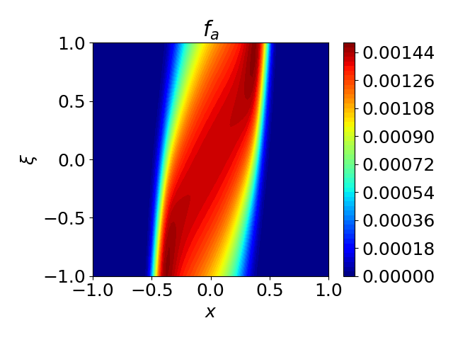

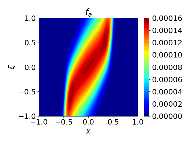
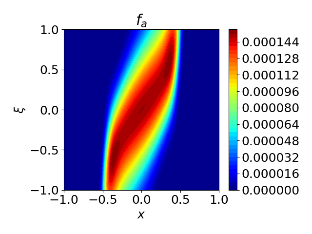
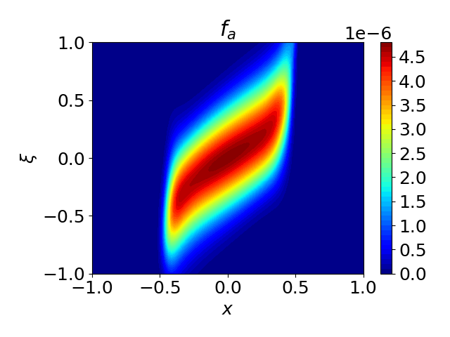

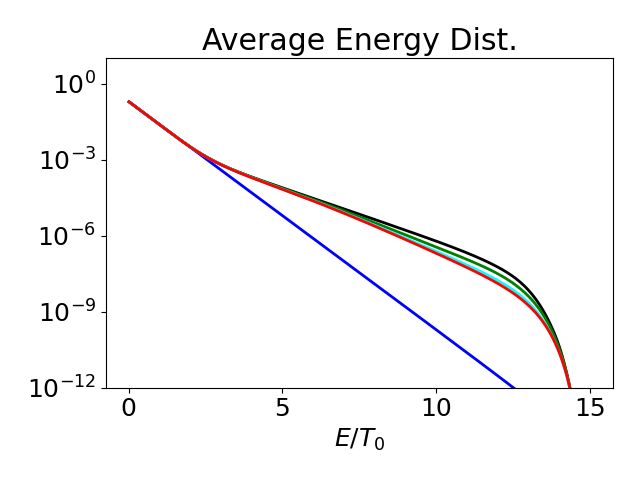
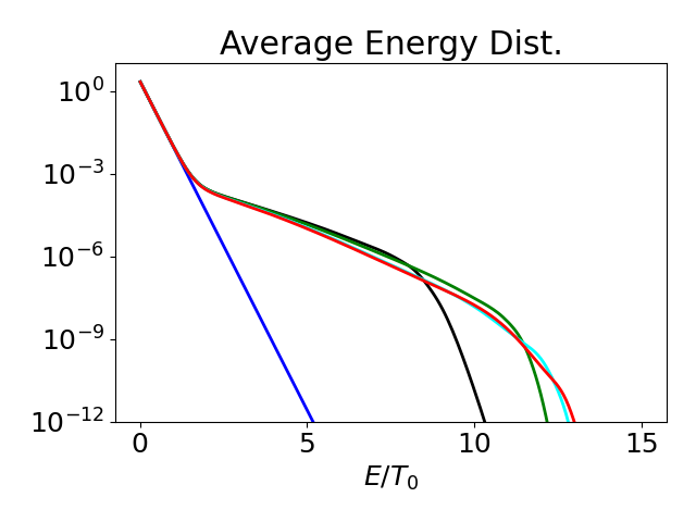
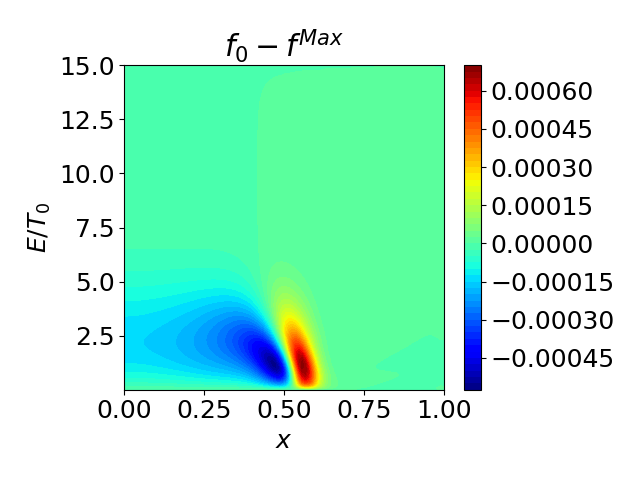
In this section it will be useful to investigate the form of the fast ion solution. We will begin by investigating the impact of the input layer described in Sec. III.2 above on the fast ion distribution. Figure 2 shows a comparison of the fast ion with and without introducing the input transform (other parameters are indicated in Table 1). Considering a cross cut of the fast ion solution in the plane at for three different energies, it is apparent that the loss of fast ions from the hot spot leads to substantial deviations from a Maxwellian distribution. In particular, noting that the temperature is maximal in the hot spot between (for the examples shown in this section, ), this is the region which would be expected to have the largest number of fast ions. For the highest energy cross cut shown [, Figs. 2(e) and (f)], it is evident that a large asymmetry in the number of ions with compared to is present. This is due to the relatively low collisionality at this energy allowing the fast ions to free stream toward the interface between the hot and cold regions. Once these fast ions reach the cold region the high collisionality results in the fast ions slowing down, which leads to maximums of the ion distribution forming at lower energies at and . These are particularly evident in the cross cut shown in Figs. 2(a) and (b). While this physics is evident for cases where the input transform is applied [Figs. 2(b), (d), (f)], and when it is not [Figs. 2(a), (c), (e)], the latter ion distribution does not precisely satisfy the symmetry , with the deviations most evident at the highest energy cross cut [compare with in Fig. 2(e), for example].
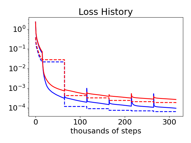
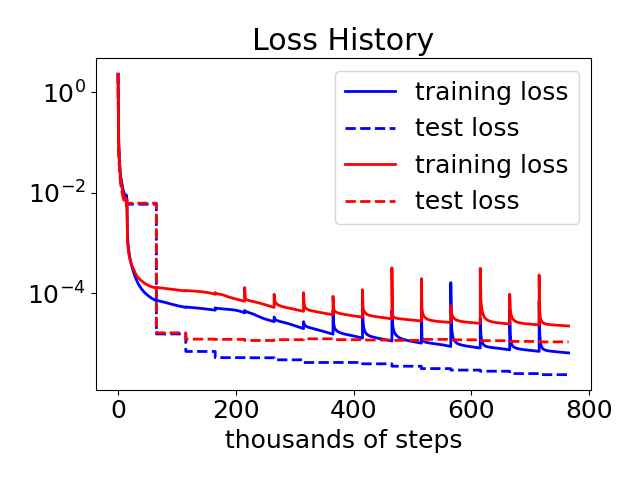
A comparison of the loss histories for the two cases is shown in Fig. 3. Here an ADAM optimizer is used for the first 15,000 epochs, and L-BFGS is used thereafter. A million training points obeying a Hammersley distribution are used in the training. After periods of 50,000 epochs of L-BFGS training, an additional 100 training points are added at locations where the residual is maximal, leading to periodic spikes in the training loss. It is evident that the loss for the case where an input transform is included is substantially reduced. Hence, the input transform provides a means of reducing the loss, and hence improving the accuracy of the solution, while exactly satisfying a known symmetry of the system. Furthermore, noting the symmetry of the solution is automatically satisfied, it is only necessary to solve for the solution in one half of the spatial domain. Hence for the remainder of this analysis we will limit the spatial domain to be between during training, where the solution for negative values of can be recovered by noting the symmetry .
IV.2 Temporal Evolution of the Fast Ion Distribution

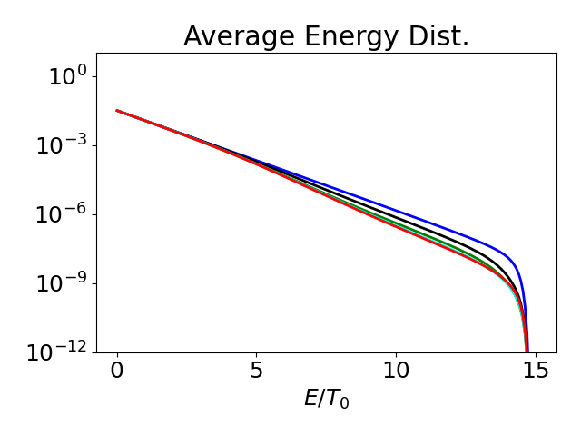
Incorporating the input transform, and training over a spatial range [see the third row of Table 1 for further details of the model], the loss history for time dependent models of the deuterium and tritium distributions are shown in Fig. 4. The test loss drops by roughly five orders of magnitude, with the tritium case achieving a slightly lower saturated loss, indicating the VFP PINN has been able to obtain an accurate solution. The pitch-angle averaged tritium distribution is shown at different spatial locations in Fig. 5 for several different time slices. Here, Fig. 5(a) indicates five time slices at , where it is evident that while the low energy bulk plasma remains approximately Maxwellian, the hot tail becomes significantly depleted by . Considering the transition region [, Fig. 5(b)], the fast ions lost from the hot spot lead to an increase in the number of fast ions in the neighboring region. After this fast ion tail forms, it slowly decreases as the fast ion tail in the hot spot decreases. Turning to a spatial location deeper into the cold region [, Fig. 5(c)], the time evolution is similar to the location, though the fast ions have slowed down substantially by the time they reach this spatial location. Fig. 5(d), shows a comparison of the fast ion distribution at the three spatial locations at . From this comparison it is clear that the magnitude of the fast ion tail decreases as is increased, though the slope of the fast ion distribution with respect to energy is similar at each spatial location.
IV.3 Legendre Moments of the Fast Ion Distribution
More insight into the fast ion solution can be gained by projecting the solution onto a basis of Legendre polynomials . In particular, noting the relations
| (15a) | |||
| (15b) | |||
| (15c) |
If the ion distribution is expanded as
| (16) |
and Eq. (16) is substituted into Eq. (15), this yields
| (17a) | |||
| (17b) | |||
| (17c) |
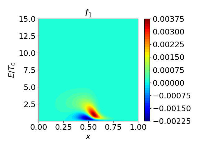
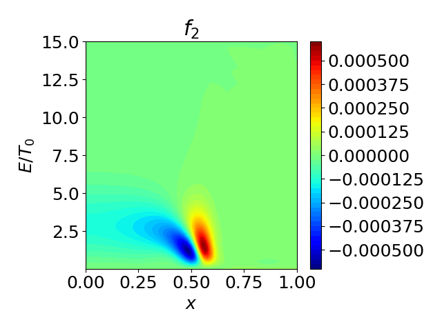
It is thus evident that the component describes the density and isotropic pressure, is linked to the spatial flux of fast ions, and describes the pressure anisotropy of the high energy ion tail. The energy and spatial dependence of the first three Legendre coefficients are shown in Fig. 6. Considering the Legendre coefficient, it is evident that the number of fast ions is reduced inside the hot spot, with a substantial surplus present in the neighboring cold region. More interestingly, the component indicates an outflow of fast ions from the hot spot at high energy, but an inflow at low energy. This inflow of low energy ions is required for particle balance as the system approaches steady state. Considering , it is evident that within the hot spot at high energy, indicating that fast ions whose direction is primarily in the direction are depleted more rapidly than those whose motion is perpendicular to the direction, with this trend reversed in the neighboring cold region.
IV.4 Comparison with Previous Results
Here we will provide a comparison of the deuterium and tritium distribution predicted by the VFP PINN with the results given in Ref. McDevitt et al. (2014b), which evaluated a nearly identical model of the fast ion distribution using a traditional numerical solver. Noting that Ref. McDevitt et al. (2014b), considered the limit of a steady state fast ion distribution, we will also modify the VFP PINN to evaluate the steady state fast ion distribution. This is done by removing the time derivative term in Eq. (2), and removing time as an input into the VFP PINN. In addition, to provide a more complete description of Knudsen layer yield reduction, we have added the parameter to the inputs of the VFP PINN, which characterizes the density gradient between the hot and cold regions. Hence, the input parameters for the steady state VFP PINN is given by [further model details are given in the fourth row of Table 1]. The loss history for the steady state VFP PINNs is shown in Fig. 7. Here, the test loss for both the tritium and deuterium VFP PINNs decreases by nearly six orders of magnitude implying that the VFP PINNs were able to successfully train.
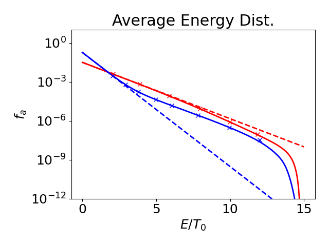
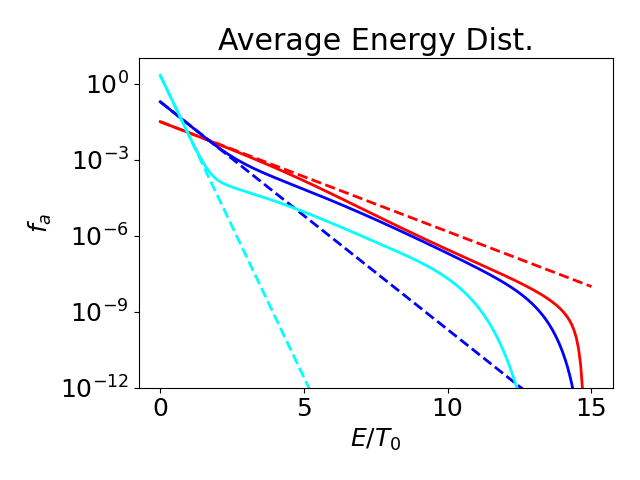
A comparison of the predicted pitch-angle averaged tritium distribution from the VFP PINN and Fig. 17 of Ref. McDevitt et al. (2014b) is shown in Fig. 8. Here, excellent agreement is evident for the ion distribution in both the hot spot (, red curves) and adjacent cold region (, red curves). While the physical parameters utilized in this comparison were matched, a handful of numerical parameters differed slightly, yielding modest differences in the predictions between the present paper and Ref. McDevitt et al. (2014b). In particular, the upper and lower energy bounds employed by the two papers are different. In the present model, the low energy boundary was taken to be , whereas Ref. McDevitt et al. (2014b) chose . Furthermore, Ref. McDevitt et al. (2014b) chose , whereas the present paper selected . While the PINN implementation could be straightforwardly modified to incorporate a low energy boundary of , we chose to demonstrate that PINNs are able to learn the ion distribution across the full range of energies. In contrast, since contributions to the fusion reactivity are negligible beyond for , we opted to restrict the energy range to . As a result of these different choices for energy ranges, Fig. 8 only includes values from Fig. 17 of Ref. McDevitt et al. (2014b) between and . Furthermore, since Ref. McDevitt et al. (2014b) used a grid based approach, where the ion distribution was only available at discreet spatial locations, a careful examination of the Maxwellian distributions shown in Fig. 17 of Ref. McDevitt et al. (2014b) indicated that the blue curves in that paper were evaluated at , rather than (using the normalization of the current paper). Finally, while both the present paper and Ref. McDevitt et al. (2014b) chose a high energy boundary condition such that the ion distribution was forced to a small value, this value differed between the two studies yielding slightly different behavior near the high energy boundary. This choice of boundary condition, however, does not strongly impact the solution at energies of interest for evaluating the fusion reactivity for temperatures greater than a few keV.
V Knudsen Layer Reactivity Reduction
In this section we will utilize VFP PINNs for the tritium and deuterium fast ion distributions to quantify how the fusion reactivity varies with hot spot parameters . To accomplish this, the fast ion distributions will be inferred using the steady state VFP PINNs described in Sec. IV.4 above. The fusion reactivity can then be evaluated from the expression
| (18) |
where is the relative velocity and is the fusion cross section parameterized by
| (19) |
Here is the center-of mass-energy , is the reduced mass, is the Gamow energy , and will be taken to have the form:
where the specific values of the coefficients and used in the present study will be taken from Ref. Bosch and Hale (1992). The six-dimensional integral defined by Eq. (18) can be simplified by expanding in Legendre coefficients, yielding Cordey et al. (1978)
| (20) |
Here, the relative velocity can be written as , the pitch-angle variable is given by , where is the angle between and , and are the Legendre coefficients defined in Eq. (16). As shown in Ref. McDevitt et al. (2014b), the sum in Eq. (20) converges rapidly, such that only a few Legendre coefficients are required for convergence. In the present study only the first two Legendre coefficients will be used. The fusion yield can then be written as:
| (21) |
where is the energy released in a given fusion reaction and is the reactivity rate.
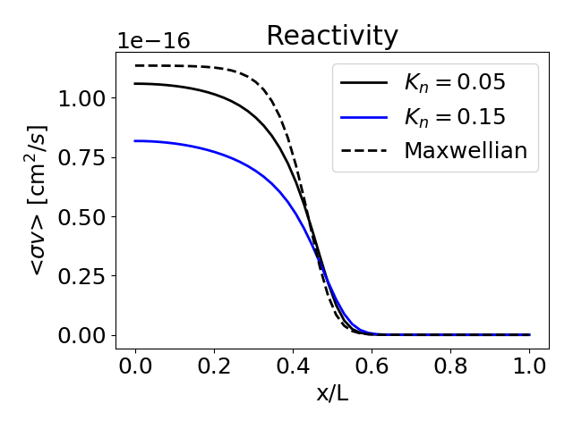
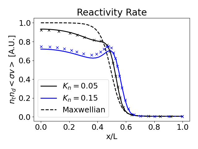
A plot of the reactivity and reactivity rate for different Knudsen numbers is shown in Fig. 9. From Fig. 9(a), it is evident that as the Knudsen number is increased the fusion reactivity is substantially decreased in the hot spot. The escaping fast ions, do however, introduce a slight increase in the reactivity in the neighboring cold region. While this increase in reactivity is small, the reaction rate is substantially increased due to the high density present in the neighboring cold region [see Fig. 9(b)]. Despite this increase in the neighboring cold region, the net fusion yield () decreases as increases [see Fig. 10 below], suggesting radiation-hydrodynamic codes which are based on the assumption of a Maxwellian plasma will overpredict the fusion reactivity at high temperatures and low densities where the Knudsen number is largest.
A comparison of the spatial fusion reaction rate profile with Fig. 24 of Ref. McDevitt et al. (2014b) is shown in Fig. 9(b). Here the solid curves represent the predictions of the VFP PINN whereas the ‘x’ markers indicate values shown in Fig. 24 of McDevitt et al. (2014b) extracted using the software Rohatgi . Due to the different normalizations employed between the present work and Ref. McDevitt et al. (2014b), both datasets have been normalized to the fusion reactivity at the center of the hot spot for a Maxwellian ion distribution. Considering first the case of a modest Knudsen number (black curve, ) the VFP PINN is in excellent agreement in the outer region of the hot spot, with good agreement also evident near the center of the hot spot. In contrast, for a large Knudsen number of , the VFP PINN predicts lower fusion yield across the entire hot spot. The origin of this systematic shift in predictions is that the low energy boundary conditions were different for the two cases. In particular, Ref. McDevitt et al. (2014b) matched the fast ion solution to a Maxwellian at for the tritium distribution, and for the deuterium distribution. In the present work we have taken for both ion distributions. As the Knudsen number is increased, deviations from a Maxwellian distribution will emerge at lower energies, which were not entirely captured by Ref. McDevitt et al. (2014b) due to the low energy boundary conditions applied in that work. In contrast, while the present study evaluates nearly the entire distribution, the fast ion model employed is only quantitatively accurate for . Hence, if deviations from a Maxwellian emerge at , these will not be accurately quantified by the collision coefficients defined by Eqs. (3). As discussed in Ref. McDevitt et al. (2014b), the fast ion model employed will thus be most accurate for cases of modest Knudsen numbers.
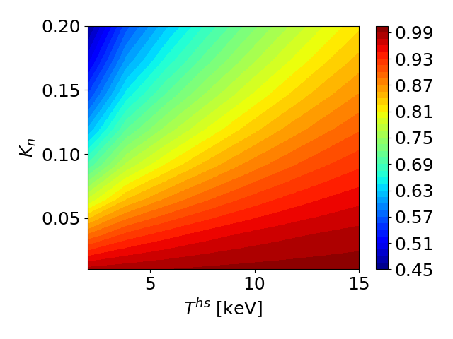
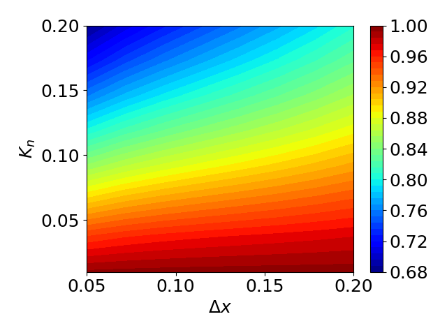
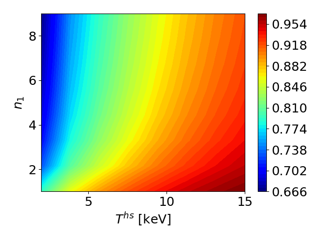
More insight into how the hot spot parameters impact Knudsen layer reactivity reduction can be gained by considering the dependence of the net fusion yield on . Here, we will evaluate the spatially integrated fusion yield as inferred from the VFP PINN, and then compare with the nominal Maxwellian value . This comparison is shown in Fig. 10. First considering the dependence of the Knudsen number , it is apparent that the spatially integrated fusion yield always decreases with increasing . This is due to larger Knudsen numbers enabling more fast ions to escape the hot spot, where they will collide with colder ions and hence will on average have a lower relative velocity, and thus lower fusion cross section. Furthermore, fast ions that escape from the hot spot will lose some of their energy to ion-electron collisions, further reducing the net fusion yield. Turning to the dependence on the hot spot temperature , the ratio increases as the temperature is increased. This is due to the location of the Gamow peak normalized to temperature decreasing as is increased. Specifically, for ions obeying a Maxwellian distribution, the energy of the Gamow peak normalized to the local temperature is given by:
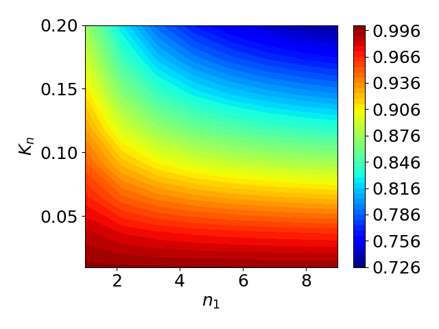
which decreases as . Since the depletion of the ion distribution at low values of is less pronounced compared to higher energies, the fractional reduction of fusion yield is also reduced. From Figs. 10(b) and (c) it is also evident that the Knudsen layer yield reduction becomes more severe as the temperature and density change between the hot spot and cold region become more extreme, or as the density region becomes sharper. This is due to the density and temperature variation providing the drive for fast ion losses, such that as is increased, or the gradient length scale is reduced, larger reductions on the fusion yield are expected.
VI Conclusions and Discussion
A physics-informed neural network was used to evaluate the fast ion tail of the tritium and deuterium distribution in the context of Knudsen reactivity layer depletion. This approach was shown to yield accurate predictions of the fast ion distribution in both the hot spot and neighboring hot region, and thus provide a robust description of fast ion depletion. A feature of the present approach is that the offline training time for each network was long, requiring approximately a day to reach a saturated level of loss on an Nvidia A100 GPU, however, the online inference time is short, typically only a microsecond per prediction. While this offline training time is expected to be long compared to most traditional fast ion solvers, a single VFP PINN is able to learn the parametric dependence of the fast ion solution, thus the model only needs to be trained once, and can then be deployed to efficiently explore the parameter space. This can be contrasted with a traditional fast ion solver, where the run time for a geometry of this complexity would be expected to be far shorter than the training time of the VFP PINN, but the traditional solver would need to be rerun for each parameter set. While the present model involves a relatively low 3-D parameter space, we do not anticipate the treatment of more comprehensive descriptions of the target hot spot (including a variable mix of materials, for example) to pose a fundamental obstacle. Such a study will be carried out in future work.
While in the present paper our focus was on Knudsen layer reactivity reduction, since the VFP PINN evaluates the time evolution of the fast ion distribution, it may be employed to evaluate other quantities of interest linked to a non-Maxwellian tail distribution. Furthermore, we do not anticipate any difficulties in extending the approach to a fast electron population. We thus expect the present approach to provide a path through which surrogate models can be developed for a range of plasma kinetic effects. The exploration of this approach for the purpose of providing a non-perturbative evaluation of the fast particle distribution for a broader range of applications will be left to future work.
Acknowledgements.
This work was supported by DOE OFES under award number DE-SC0024634. The authors acknowledge the University of Florida Research Computing for providing computational resources that have contributed to the research results reported in this publication.References
- Clark et al. (2011) D. Clark, S. Haan, A. Cook, M. Edwards, B. Hammel, J. Koning, and M. Marinak, Physics of Plasmas 18 (2011).
- Johnson et al. (2020) M. G. Johnson, B. M. Haines, P. Adrian, C. Forrest, J. Frenje, V. Y. Glebov, W. Grimble, R. Janezic, J. Knauer, B. Lahmann, et al., High Energy Density Physics 36, 100825 (2020).
- Rosenberg et al. (2014) M. Rosenberg, A. Zylstra, F. Séguin, H. Rinderknecht, J. Frenje, M. Gatu Johnson, H. Sio, C. Waugh, N. Sinenian, C. Li, et al., Physics of Plasmas 21 (2014).
- Rinderknecht et al. (2015) H. G. Rinderknecht, M. Rosenberg, C. Li, N. Hoffman, G. Kagan, A. Zylstra, H. Sio, J. Frenje, M. G. Johnson, F. Séguin, et al., Physical Review Letters 114, 025001 (2015).
- Hartouni et al. (2023) E. Hartouni, A. Moore, A. Crilly, B. Appelbe, P. Amendt, K. Baker, D. Casey, D. Clark, T. Döppner, M. Eckart, et al., Nature Physics 19, 72 (2023).
- Chapman et al. (1990) S. Chapman, T. G. Cowling, and D. Burnett, The mathematical theory of non-uniform gases: an account of the kinetic theory of viscosity, thermal conduction and diffusion in gases (Cambridge university press, 1990).
- Braginskii (1958) S. Braginskii, Sov. Phys. JETP 6, 358 (1958).
- Spitzer Jr and Härm (1953) L. Spitzer Jr and R. Härm, Physical Review 89, 977 (1953).
- Epperlein and Short (1991) E. Epperlein and R. Short, Physics of Fluids B: Plasma Physics 3, 3092 (1991).
- Schurtz et al. (2000) G. Schurtz, P. D. Nicolaï, and M. Busquet, Physics of plasmas 7, 4238 (2000).
- Chapman et al. (2021) D. Chapman, J. Pecover, N. Chaturvedi, N. Niasse, M. Read, D. Vassilev, J. Chittenden, N. Hawker, and N. Joiner, Physics of Plasmas 28 (2021).
- Miniati and Gregori (2022) F. Miniati and G. Gregori, Scientific Reports 12, 11709 (2022).
- Henderson (1974) D. B. Henderson, Physical Review Letters 33, 1142 (1974).
- Petschek and Henderson (1979) A. Petschek and D. Henderson, Nuclear Fusion 19, 1678 (1979).
- Molvig et al. (2012) K. Molvig, N. M. Hoffman, B. Albright, E. M. Nelson, and R. B. Webster, Physical review letters 109, 095001 (2012).
- McDevitt et al. (2014a) C. McDevitt, X.-Z. Tang, Z. Guo, and H. Berk, Physics of Plasmas 21 (2014a).
- Kagan et al. (2015) G. Kagan, D. Svyatskiy, H. Rinderknecht, M. Rosenberg, A. Zylstra, C.-K. Huang, and C. McDevitt, Physical review letters 115, 105002 (2015).
- Garland et al. (2022) N. A. Garland, H.-K. Chung, M. C. Zammit, C. J. McDevitt, J. Colgan, C. J. Fontes, and X.-Z. Tang, Physics of Plasmas 29 (2022).
- Rinderknecht et al. (2018) H. G. Rinderknecht, P. Amendt, S. Wilks, and G. Collins, Plasma Physics and Controlled Fusion 60, 064001 (2018).
- Frenje (2020) J. Frenje, Plasma Physics and Controlled Fusion 62, 023001 (2020).
- Crilly et al. (2022) A. Crilly, B. Appelbe, O. Mannion, W. Taitano, E. Hartouni, A. Moore, M. Gatu-Johnson, and J. Chittenden, Nuclear Fusion 62, 126015 (2022).
- Kagan et al. (2019) G. Kagan, O. Landen, D. Svyatskiy, H. Sio, N. Kabadi, R. Simpson, M. Gatu Johnson, J. Frenje, R. Petrasso, R. Shah, et al., Inference of the electron temperature in inertial confinement fusion implosions from the hard x-ray spectral continuum (2019).
- Larroche (2012) O. Larroche, Physics of Plasmas 19 (2012).
- Taitano et al. (2015) W. T. Taitano, L. Chacón, A. Simakov, and K. Molvig, Journal of Computational Physics 297, 357 (2015).
- Karniadakis et al. (2021) G. E. Karniadakis, I. G. Kevrekidis, L. Lu, P. Perdikaris, S. Wang, and L. Yang, Nature Reviews Physics 3, 422 (2021).
- Sun et al. (2020) L. Sun, H. Gao, S. Pan, and J.-X. Wang, Computer Methods in Applied Mechanics and Engineering 361, 112732 (2020).
- Lagaris et al. (1998) I. E. Lagaris, A. Likas, and D. I. Fotiadis, IEEE transactions on neural networks 9, 987 (1998).
- Karpatne et al. (2017) A. Karpatne, G. Atluri, J. H. Faghmous, M. Steinbach, A. Banerjee, A. Ganguly, S. Shekhar, N. Samatova, and V. Kumar, IEEE Transactions on knowledge and data engineering 29, 2318 (2017).
- Lusch et al. (2018) B. Lusch, J. N. Kutz, and S. L. Brunton, Nature communications 9, 1 (2018).
- Wang et al. (2020) R. Wang, K. Kashinath, M. Mustafa, A. Albert, and R. Yu, in Proceedings of the 26th ACM SIGKDD International Conference on Knowledge Discovery & Data Mining (2020), pp. 1457–1466.
- Raissi et al. (2019) M. Raissi, P. Perdikaris, and G. E. Karniadakis, Journal of Computational physics 378, 686 (2019).
- Tang et al. (2014a) X.-Z. Tang, H. Berk, Z. Guo, and C. McDevitt, Physics of Plasmas 21, 032707 (2014a).
- McDevitt et al. (2014b) C. McDevitt, X.-Z. Tang, Z. Guo, and H. Berk, Physics of Plasmas 21, 032708 (2014b).
- Braginskii and Leontovich (1965) S. Braginskii and M. Leontovich, Reviews of plasma physics (1965).
- Tang et al. (2014b) X.-Z. Tang, C. McDevitt, Z. Guo, and H. Berk, EPL (Europhysics Letters) 105, 32001 (2014b).
- (36) A. Rohatgi, Webplotdigitizer, https://automeris.io/WebPlotDigitizer.
- Bosch and Hale (1992) H.-S. Bosch and G. Hale, Nuclear fusion 32, 611 (1992).
- Cordey et al. (1978) J. Cordey, K. Marx, M. McCoy, A. Mirin, and M. Rensink, Journal of Computational Physics 28, 115 (1978).