Revealing Decurve Flows for Generalized Graph Propagation
Abstract
This study addresses the limitations of the traditional analysis of message-passing, central to graph learning, by defining generalized propagation with directed and weighted graphs. The significance manifest in two ways. Firstly, we propose Generalized Propagation Neural Networks (GPNNs), a framework that unifies most propagation-based graph neural networks. By generating directed-weighted propagation graphs with adjacency function and connectivity function, GPNNs offer enhanced insights into attention mechanisms across various graph models. We delve into the trade-offs within the design space with empirical experiments and emphasize the crucial role of the adjacency function for model expressivity via theoretical analysis. Secondly, we propose the Continuous Unified Ricci Curvature (CURC), an extension of celebrated Ollivier-Ricci Curvature for directed and weighted graphs. Theoretically, we demonstrate that CURC possesses continuity, scale invariance, and a lower bound connection with the Dirichlet isoperimetric constant validating bottleneck analysis for GPNNs. We include a preliminary exploration of learned propagation patterns in datasets, a first in the field. We observe an intriguing “decurve flow” - a curvature reduction during training for models with learnable propagation, revealing the evolution of propagation over time and a deeper connection to over-smoothing and bottleneck trade-off.
1 Introduction
Propagation of vertex features is central to various graph models, including message-passing models (MPNNs) and graph transformers (GTs).
MPNNs pass features by the graph structure of incoming data, inherently capturing characteristics of the underlying graph structure Hamilton et al. (2017); Veličković et al. (2018); Monti et al. (2017). Propagation of MPNNs is carefully inspected by analyzing its expressivity and geometric properties based on undirected and unweighted graphs. In detail, the expressive power of message-passing is bounded by the first-order Weisfeiler-Lehman test (1-WL)Xu et al. (2019); Chen et al. (2019). Furthermore, MPNNs suffer from over-squashing Alon and Yahav (2020) and over-smoothing Chen et al. (2020); Oono and Suzuki (2019) phenomena due to the undesirable geometric properties of the graph structures (eg. molecule, knowledge graph) like bottlenecks and complete graphs.
On the other hand, graph transformers determine the propagation of features with “attention” Vaswani et al. (2017). Pioneering methods directly apply self-attention on graphs, suffering a lack of structural information Dwivedi and Bresson (2021) and can be potentially improved by injecting additional positional/structural encodings Kreuzer et al. (2021a); Rampášek et al. (2022); Chen et al. (2022); Ma et al. (2023). Although GTs have shown superior performance on various benchmarks and diverse heuristics, a clear understanding of how they gain their power remains elusive Cai et al. (2023). Specifically, GTs are considered propagating messages with a undirected-unweighted complete graph Shirzad et al. (2023a). However, a random walk on complete graph would soon converges to stable distribution which implies severe over-smoothing Giraldo et al. (2022), contradicting the empirical success of GTs.
In this study, we demonstrate that the limitation of existing analysis on message propagation largely stems from the traditional focus on defining propagation within the realm of undirected and unweighted graphs. Challenging conventional boundaries, we conceptualize the generalize propagation with directed and weighted graphs. The significance of this generalization manifest in two ways.
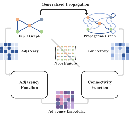
Firstly, we introduce Generalized Propagation Networks (GPNNs), which unify GTs, MPNNs, and their variants by adopting directed, weighted propagation graphs. Central to GPNNs is the adjacency function, mapping adjacency matrices to vertex pair embeddings, and the connectivity function, converting these embeddings and vertex features into scalar values. This framework advances the analysis of propagation in graph models by its inherent ability to model “attention”, which is neglected with undirected and unweighted modeling. For completeness, we show that GPNNs’ expressiveness is determined by their adjacency function theoretically. Furthermore, we provide a taxonomy (see Appendix E.1) for the models that belongs to GPNN family and showcase the high-level design choice in literature. Through empirical evaluations within the design space, we show the impact of adjacency and connectivity function and pinpointing the most effective configurations as well as ineffective ones.
Secondly, we propose the Continuous Unified Ricci Curvature (CURC), extending the celebrated Ollivier-Ricci (OR) Curvature to directed and weighted graphs Ollivier (2009). CURC is defined by Wasserstein distance between mean transition probabilities centered at each vertex and an asymmetric distance for vertex pairs. During the derivation of CURC, we give a stronger version of Kantorovich-Rubinstein duality, which not only serves as the theoretical basis for our design of reciprocal edge weight, but also enables a wider class of valid distance function to create different graph curvatures based on Riemannian Geometry. Furthermore, three benign properties of CURC are demonstrated, which are particularly designed for generalized propagation graphs: (i) continuity, which enables smooth variation of the curvature with respect to the propagation graphs; (ii) unity with Ollivier-Ricci Curvature when the input graph is undirected and unweighted, when and coexist and both ; and (iii) a lower bound linking CURC with the Dirichlet Isoperimetric Constant, validating the use of CURC in analyzing bottlenecks on graphs.
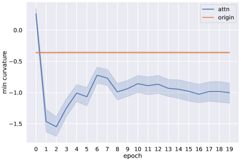
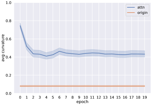
We analyze the geometric property of the generalized propagation for models with learnable propagation during training, which has been carried out for undirected-unweighted propagation with OR curvature by Topping et al. (2022). First in the field, we spotted the intriguing “decurve flow” phenomenon – a curvature reduction propagation graph evolution observed in multiple models, including the stat-of-the-art, during early stage in training. In contrast to rewiring Topping et al. (2022), which increases curvature and reduces bottlenecks, generalized propagation graph of inspected models starts from a distribution of high curvatures and gradually decurves. This suggests a possible explanation of GTs performance: starting from a extreme curved state, GTs solves over-smoothing vs trade-off with respect to data.
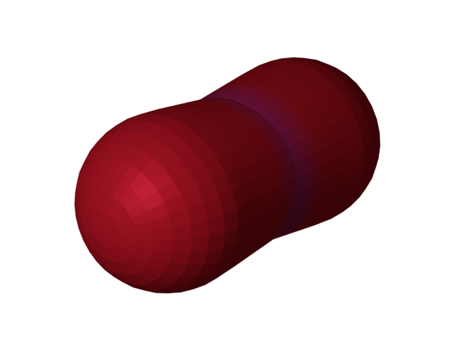

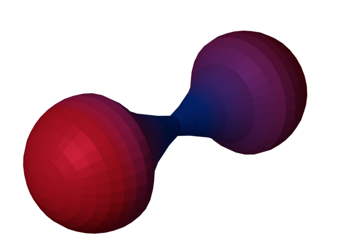
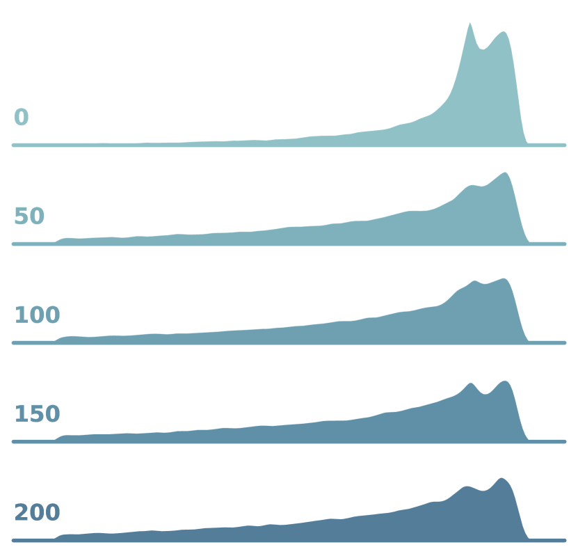
This visual serves as an analogy for the curvature decrease observed in Generalized Propagation Neural Networks (GPNNs) with learnable propagation. The proposed Continuous Uniform Ricci Curvature (CURC) are applied to characterize this “decurve flow” observed across various models. Dark-blue and red represent regions of negative and positive curvature, respectively
2 Directed and Weighted Propagation
This section challenges the convention by defining message propagation on directed-weighted graphs. We show that directed-weighted propagation inherently provides insight to the “attention” mechanism in MPNNs. This analysis is extended towards a general graph model framework - GPNN, characterizing various propagation based methods. We finish this section with a discussion on its design space and an exhibition of GPNNs expressivity.
Preliminary
In this work, we concern machine learning algorithms on undirected graphs characterized by two sets, namely the vertices and the edges . Given the indexes of the vertices, the structure of the graph can also be represented by its adjacency matrix , where iff and zero otherwise. Each vertex and edge could be associated with attributes and . The intermediate hidden variables passing between layers are denoted as . A graph network model usually contains multiple layers marked as .
Generalized Propagation
We consider message propagation on weighted-directed graph , where denotes the connectivity: . The connectivity models the amount of information that is passed along with a specific edge (eg. “attention”). In fact, the concept of weighted propagation is common and can be introduced to MPNNs by refining its definition (see Appendix C.1)
| (1) | ||||
where is a scalar function that models the connectivity. This formulation is standard in most MPNNs Kipf and Welling (2017); Monti et al. (2017); Veličković et al. (2018); Bresson and Laurent (2018). Previous analyses over message passing are based on the summation over neighbors, overlooking the important affect of connectivity.
GPNNs
To obtain a general formulation, we make extentions: (1) summation over all vertices. (2) an adjacency function , defined as a permutation equivariant mapping from the adjacency matrix and edge feature (if available) to its embedding . (3) the connectivity function which depend on adjacency feature and along with vertex features. The resulting formulation contains four steps for each layer,
| (2) | ||||
where indicates the element of the input matrix/tensor.
2.1 GPNN Design Space
In Appendix E.2 we show existing methods belong to GPNNs by casting their formulation with GPNNs’ adjacency and connectivity function. GPNNs cover a wide range of propagation-based models, making them excellent guidelines for taxonomy (see Appendix E.1). Here we highlight several important design choices.
Multi-head v.s. Single-head
pinpointing the question of whether multiple propagation graphs should be used in each GPNN layer. When multi-head is adopted, , and will be specific to each head as , and . The multi-head approach is adopted commonly with attention mechanisms.
Local v.s. Non-Local v.s. Global Propagation
can be identified based on the constraints imposed by the input graph. Local propagation constraints the propagation graph to be a weighted version of the input graph, which is typical for MPNNs. Global propagation poses no constraint to the propagation graph, characterizing most GTs. Non-local propagation, making the propagation graph a super graph of the input graph, includes additional edges but does not form a complete graph to balance cost and expressiveness, incorporating techniques like graph-rewiring, polynomial spectral GNNs, diffusion-enhanced GNNs, and efficient GTs or MPNNs with virtual nodes.
Static v.s. Dynamic Propagation
static mode denotes that all layers in GPNNs are sharing the same propagation graph. In contrast, the dynamic mode indicates that different propagation graphs are used in different layers. This is typically implemented by evolving the connectivity across layers.
Feature-independent v.s. Feature-dependent Propagation
The propagation graph can be generated in two ways: depending on the node features, referred to as feature-dependent (Feat. Dep.) propagation, commonly seen in models with attention or gating mechanisms. Otherwise, the propagation is referred to as feature-independent (Feat. Ind.) propagation. The adjacency function , as the essential component in GPNNs, interprets the topological information contained in the adjacency matrix for the connectivity function. The adjacency functions can be as simple as performing normalization on adjacency matrix or the Laplacian matrix , as seen in many MPNNs. More complicated designs, such as computing power series of () (polynomial spectral/diffusion GNNs Defferrard et al. (2016); Gasteiger et al. (2019); Frasca et al. (2020), GRIT Ma et al. (2023)) or performing eigendecomposition on () Kreuzer et al. (2021a); Hussain et al. (2022), can explore richer topological information and facilitate connectivity function to generate more expressive propagation graphs.
2.2 Expressiveness of GPNNs
GPNNs subsume models with various expressiveness. However, by abstracting away the exact adjacency and mild assumption over connectivity function (MLPs), we deliver two propositions by inducting a common routine for propagation-based models expressivity assessment. To reach the upper-bounded expressiveness for both propositions, a sufficient number of heads, MLPs with a sufficient layer and width for the connectivity function, and an update function are required. First, we consider the GPNNs with static propagation for a sufficient number of heads and layers, referred to as static GPNNs.
Proposition 2.1.
(Static GPNNs) For a static GPNN model with a fixed adjacency feature and sufficient heads and layers, the expressiveness is upper-bounded by the color refinement iteration
| (3) |
The proof the proposition 2.1 is provided in Appendix B.2. This expressiveness result could be induced by existing expressivity proof in propagation-based GNNs. This proposition assured an expressiveness upper bound for models in GPNN families by solely inspecting their adjacency function.
Generally, we consider the unusual case when multiple adjacency function is applied, rotating among layers, eg. Rampášek et al. (2022).
Proposition 2.2.
(Dynamic GPNNs) Suppose a Layer-recurrent GPNN model M has a layer-dependent adjacency embedding repeats every layer: . With sufficient heads and layers, by stacking of such repetition, the expressiveness of M is upper-bounded by the color refinement iteration
| (4) |
We refer readers to Appendix B.2 for detailed proof. This proposition justified those approaches introducing multiple adjacency functions for different layers: the overall expressiveness is not weaker than the ones using any one of the adjacency functions alone. This proposition provides a strong theoretical foundation for the usage of dynamic propagation designs in GPNNs.
3 Continuous Unified Ricci Curvature
In the previous section, we generalize message propagation with directed-weighted graphs and carry out a general framework that characterizes various propagation-based graph models. In this section, we introduce the Continuous Unified Ricci Curvature (CURC) designed explicitly for analyzing GPNNs’ weighted-directed propagation graph. Notably, we propose a stronger version of Kantorovich-Rubinstein duality, which serves as the theoretical basis for our design of reciprocal edge weight and enables a broader class of valid distance functions. Later, we discuss the connection between optimal transport and information propagation on graphs. Finally, we finish by analyzing the properties of CURC, including a lower bound connecting the Dirichlet isoperimetric constant and CURC.
3.1 Preliminaries for CURC
To facilitate comprehension of readers and maintain the notation consistency with earlier works on curvatures, we utilize function notation to describe CURC. For example, we interpret as a function where is equivalent to in Eq. 1. To avoid confusion with the notations in previous sections, we use instead of specifically in for CURC. Note that, for CURC, we only consider the absolute value of . We assume all propagation graphs in this section to be strongly-connected weighted-directed finite graphs with vertices, except otherwise specified. Let the random walk matrix be defined by , where . In the following discussions, we abuse the notation of to keep in line with other function-form variables, where we denote as . We construct CURC based on the curvature proposed by Ozawa et al. (2020) and Lin-Liu-Yau Ricci Curvature Lin et al. (2011).
3.2 Construction of CURC
According to the Perron-Fronbenius Theorem Kirkwood and Kirkwood (2020), for a finite strongly-connected weighted-directed graph , there exists a strictly positive left eigenvector of the corresponding random walk matrix (Perron-Frobenius left eigenvector). By normalizing , we state the following concept of Perron measure, which also corresponds to the stationary distribution for the random walk matrix .
Definition 3.1.
(Perron measure) For , let be its Perron-Frobenius left eigenvector. The Perron measure is defined by
Definition 3.2.
(Mean transition probability kernel) Let be the perron measure defined on graph . The mean transition probability kernel is defined by
| (5) |
where and for fixed .
Here, we can easily induce that by checking and . Intuitively, contains the information of random walks from to . We aim to define curvature for weighted-directed graphs with Wasserstein distance by optimal transpor. We will use this mean transition probability kernel to construct initial mass distribution for the optimal transport Ozawa et al. (2020). In order to reduce the optimal transport problem to linear programming, K-R duality is essential. Conventionally, we require a distance function to be non-negative, definite, symmetric and satisfies the triangle inequality. In the following, we propose a version of K-R duality that requires a weaker condition on the distance function of graph , excluding the symmetry restriction.
Definition 3.3.
(Coupling) Suppose and to be two probability distribution on finite sets and respectively. Let denotes the set of couplings between and . We say is a coupling if
Theorem 3.4.
(K-R duality) Let be a graph with (asymmetric) distance function satisfying triangle inequality and admits . Then for probability measure , the Kantorovich-Rubinstein duality holds. Namely,
| (6) |
where is a coupling between and , if for all , .
Proof of Theorem 3.4 is given in Appendix A.6. Additionally, for computational intensive scenario, we offer two lower-bound estimations of CURC under distinct assumptions in Appendix A.26 and A.29, with computational costs of and , respectively. Here, we define the reciprocal edge weight to construct such asymmetric distance function.
Definition 3.5.
(Reciprocal edge weight) Let be a small positive real value, then the -masked reciprocal edge weight is defined by
Definition 3.6.
(Reciprocal distance function) The -masked reciprocal distance function is defined by
In particular, is a possibly asymmetric distance function on , which is consistent with directed-weighted graph propagation in GPNNs. Now we are ready to drive the definition of CURC. Attention should be placed to handle the singularity issue of reciprocal distance. We use an extra definition wtih to define with limit.
Definition 3.7.
(CURC) Let be a graph equipped with the -masked weighted reciprocal distance function . For distinct , we define the -masked Continuous Unified Ricci Curvature by
where the Wasserstein distance is based on . The corresponding Continuous Unified Ricci Curvature (CURC) is defined by
3.3 Optimal Transport of Information
Here, we share intuition over optimal transport of information. Existing applicaiton of optimal transportation in a message-passing on graphs is investigated by Topping et al. (2022), utilizing Ollivier-Ricci (OR) curvature. For vertices , OR-curvature, represented as , evaluates the ratio of Wasserstein to graph distance, signifying the cost of moving uniform mass across edges. In this framework, information from each vertex diminishes as it spreads to neighboring vertices due to the nested aggregation function. Such diminishing impact is akin to the cost in Wasserstein distance. By normalizing this, we assert OR-curvature as a metric to measure the difficulty of information transport between vertices. This motivates us to develop CURC based on optimal transport.
3.4 Properties of CURC
Proposition 3.8.
The Continuous Unified Ricci Curvature admits the following properties:
-
•
(Unity) For connected unweighted-undirected graph , for any vertex pair , we have , where is the Ollivier-ricci curvature.
-
•
(Continuity) If we perceive as a function of , then is continuous w.r.t. entry-wise.
-
•
(Scale invariance) For strongly-connected weighted-directed graph , when all edge weights are scaled by an arbitrary positive constant , the value of for any vertex pair is invariant.
Detailed proof Proposition 3.8 is given in Appendix A.14. The Unity and Continuity properties collectively establish CURC as a continuous extension of the canonical Ollivier-Ricci curvature, as originally introduced in Ollivier (2009). Scale invariance is a crucial property for CURC being a measure of bottlenecks on the propagation graph. Intuitively, uniformly scaling of edge weight does not change the dynamics of information on the propagation graph, leading to a robust bottlenecks or oversquashing measure on the graph.
Furthermore, we establish how CURC can be perceived as a measure of bottlenecks phenomenon with the help of the so-called Dirichlet isoperimetric constant, which is the direct extension of Cheeger constant into strongly-connected weighted-directed graphs. Cheeger constant has been widely used to measure bottlenecks of GNN messsage-passing on undirected-unweighted graphs due to its connection with community clustering. In Topping et al. (2022), they established the connection between Balanced Forman curvature with Cheeger constant using spectral properties. Likewise, we derive similar property between CURC and Dirichlet isoperimetric constant to conclude our theoretical discussion of CURC and its connection to bottlenecks.
Definition 3.9.
(Boundary Perron-measure) For a non-empty , its Boundary Perron-measure is defined as
where and .
Definition 3.10.
(Dirichlet isoperimetric constant) The Dirichlet isoperimetric constant on a non-empty set is defined by
Theorem 3.11.
Let and . Fix , we assume for some and for some . For , we further assume that for all , . Then the Dirichlet isoperimetric constant admits the following lower bound:
Proof of Theorem 3.11 is given in Appendix A.25. Same as its counterpart in undirected-unweighted graphs, a small Dirichlet isopermetric constant indicates higher probability of bottlenecks on propagation graph. For a fixed vertex , a large value of for implie a large value of , which results in a larger lower bound for the Dirichlet ioperimetric constant according to Theorem 3.11. Combined with Proposition 3.8, CURC constitues a proper instrument for measuring the bottleneck phenomenon on propagation graphs within our GPNN framework. For better visualization, we present the CURC distributions of our GPNN models in the later experiments.
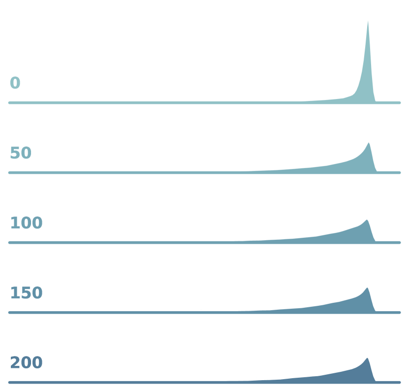
(a) SAN
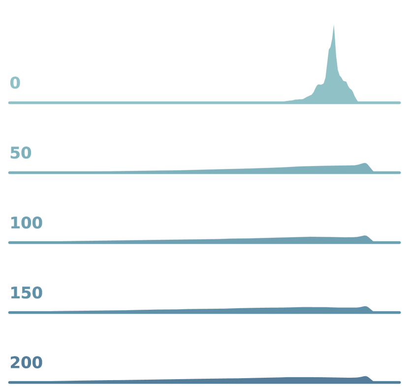
(b) Graphormer
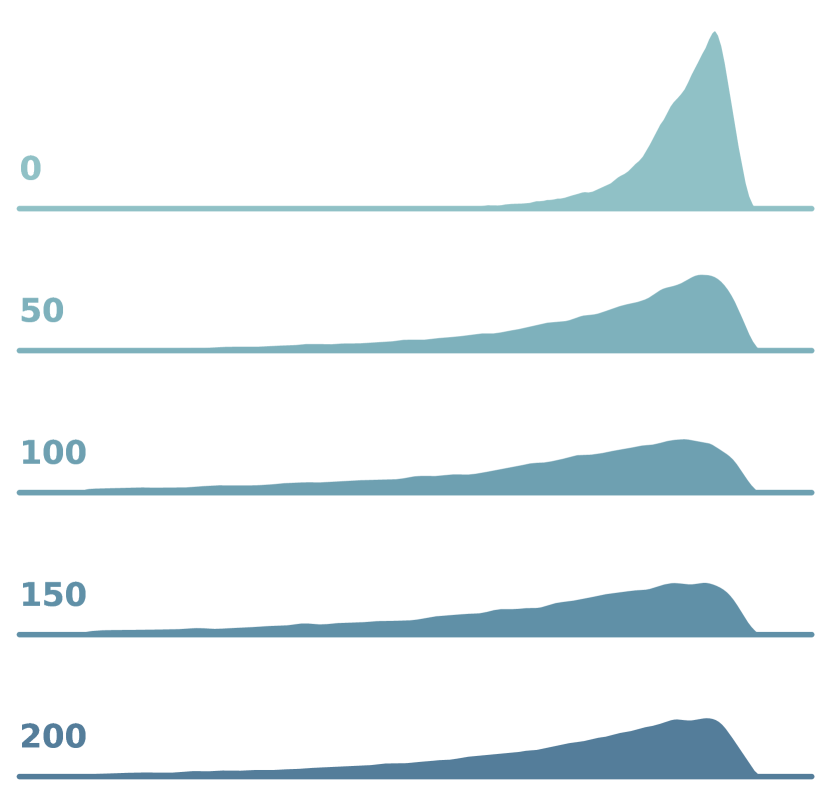
(c) GRIT
(d) GPNN-PE
4 “Decurve Flow” Phenomenon
The proposed Continuous Unified Ricci Curvature (CURC) allows for in-depth analysis of geometric properties in GPNN variants, particularly focusing on Graph Transformers (GTs). This analysis aids in identifying optimal propagation graph structures, enhancing our understanding of graph learning and informing the design of new GPNN models.
4.1 Analyzing the Learning Dynamic on CURC
To better understand the behavior of GTs and exploring potential learning patterns, we analyze the trend in CURC distributions of the propagation graphs during training.
We consider three classical graph transformers, Graphormer Ying et al. (2021), SANs Kreuzer et al. (2021b), GRIT Ma et al. (2023) as well as a simplified, feat. ind. variant of GRIT, namely GPNN-PE (details in Appx. F.1).
We first visualize the kernel density estimate (KDE) plots of CURC distributions on sampled graphs from ZINC datasets on 0, 50, 100, 150 and 200 training epochs (as shown in Fig. 3). Based on the visualization, we reveal that these models all exhibit similar learning patterns: the propagation graphs at the initial stage resemble a smoothed complete graph resulting in a strongly right-skewed CURC distribution with nearly all positive curvatures. As the training epochs increase, the learned propagation graphs gradually shift towards the left, indicating the geometric patterns learned from the graphs.
We name this phenomenon as decurve flow. In fact, Decurve flow can be connected to the recent study on the relationship between over-smoothing and over-squashing Giraldo et al. (2022). Giraldo et al. (2022) reveal that small curvature values might cause the over-squashing problem, whereas, over-large curvatures might, on the other hand, lead to over-smoothing issues. Correspondingly, we conjecture that, even though start with random initialized complete propagation graphs, GTs learn to diminish the CURC to alleviate over-smoothing. In other words, there might exist an optimal propagation graph, balancing the over-squashing and over-smoothing, which is potentially identifiable via further in-depth analysis on the CURC distributions.
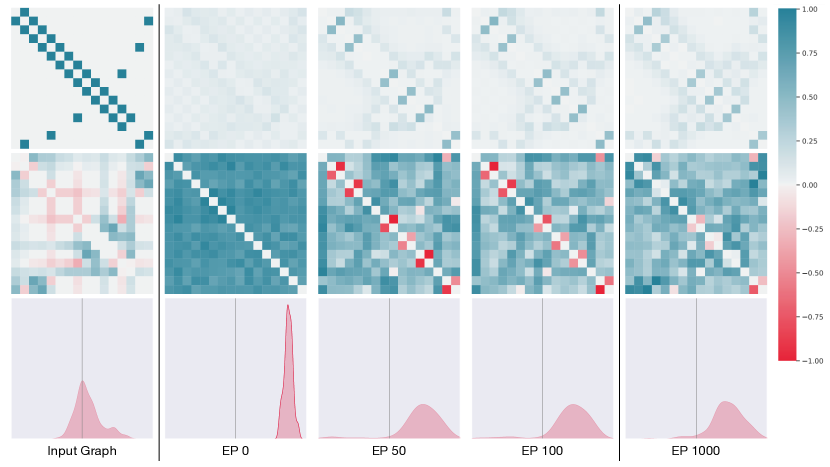
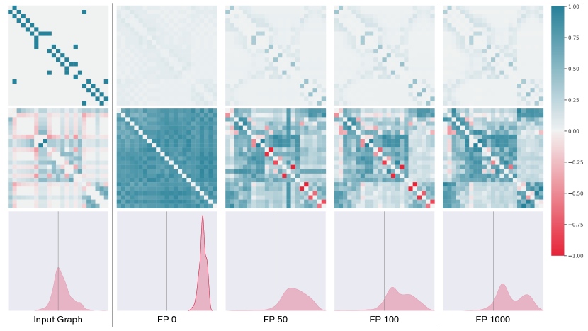
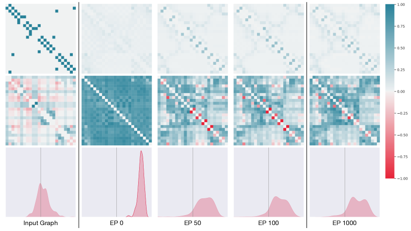
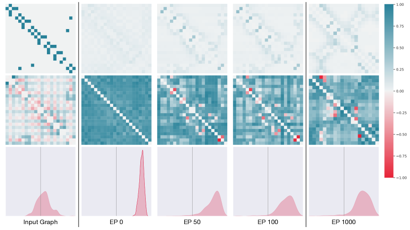
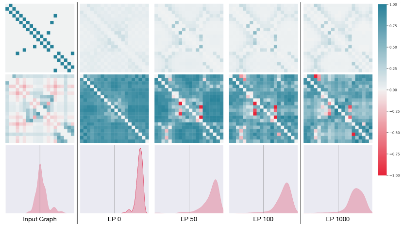
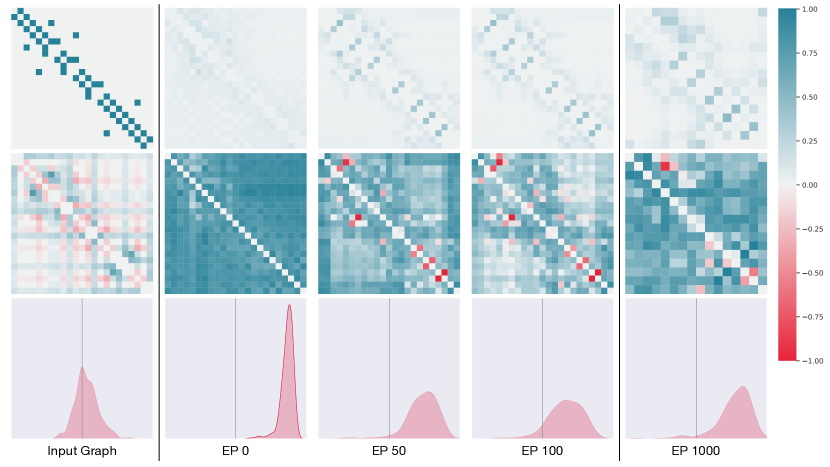
4.2 In-depth exploration on propagation matrices, CURC maps and CURC distributions
To further understand decurve flow, we go beyond the distribution and visualize propagation matrices (1st row), the corresponding CURC maps (2nd row) as well as the CURC distributions (3rd row) of GPNN-PE on 6 graphs from ZINC (shown in Fig 4). From the visualization, we observe that the CURC maps of GPNN-PE, from all large positive values, gradually learn small and even negative CURC values for certain node pairs. These observations match our conjecture: a well-optimized propagation matrix might deliberately diminish the information transport between two nodes, in order to prevent over-smoothing.
5 Navigating GPNN Design
GPNN framework unifies GTs, MPNNs and their variants by two key components, adjacency function and connectivity function. Here, we first conduct a series of in-depth exploratory experiments on ZINC datasets Dwivedi et al. (2022a) to explore their design spaces and reveal the effective configurations as well as ineffective ones. Then we conduct thorough experiments on five datasets from Dwivedi et al. (2022a) and two from Dwivedi et al. (2022b) to properly justify our hypothesis on the configurations.
5.1 Designs of Connectivity Functions
In Sec.2.1, we discuss the taxonomy of the connectivity functions in our GPNN framework. Here, we explore the impact of each potential design on the connectivity functions and identify the essential configurations. Here, we conduct a thorough comparison experiment on ZINC-12K Dwivedi et al. (2022a) for different variants of GPNNs with different configurations: (1) feat. dep. ✓v.s., feat. ind. ✗; (2) dynamic ✓v.s. static ✗; (3) multi-head ✓v.s. single head ✗; as well as (4) global ✓v.s. local✗; The experimental results are shown in Table 1.
Empirically, compared to the full configuration (all ✓), changing feat. dep. to feat. ind. only leads to a statistically insignificant performance drop. This empirical finding matches our theoretical analysis in Sec. 2.2: the adjacency function is the dominant component of the expressive power on distinguishing non-isomorphism graphs, whereas the feat. ind. counterpart is much less essential. This drives us to conduct further ablation study based on this variant. From the empirical results, changing global to local, dynamic to static and multi-head to single-head will demonstrate different levels of decline in efficacy. The comparisons against two existing MPNNs demonstrate similar findings and also hint the importantness of the choices of adjacency functions.
| ZINC (MAE) | Local✗ Global✓ | Static✗ Dynamic✓ | Single ✗ Multi. ✓ Head. | Feat. Ind. ✗ Cond. ✓ | Adj. Func. | Model |
| ✓ | ✓ | ✓ | ✓ | 21-RRWP* | GRIT | |
| ✓ | ✓ | ✓ | ✗ | 21-RRWP | GPNN-PE | |
| ✓ | ✗ | ✓ | ✗ | 21-RRWP | + static | |
| ✓ | ✓ | ✗ | ✗ | 21-RRWP | + 1-head | |
| ✗ | ✓ | ✓ | ✗ | 21-RRWP | + local | |
| ✗ | ✗ | ✗ | ✗ | RWSE+1-RRWP | (GINE+RWSE) | |
| ✗ | ✗ | ✗ | ✗ | 1-RRWP | (GIN) | |
| *: 21-RRWP will naturally include RWSE with 21-order. | ||||||
| Adjacency Function | ZINC (MAE) |
| 21-RRWP | |
| SPD | |
| pair-LapPE | |
| 1-RRWP |
5.2 Designs of Adjacency Function
Following the previous exploration, we would like to verify the essentiality of the adjacency function on the empirical results. Specifically, using GPNN-PE as the platform for comparison, we conduct experiments on ZINC, comparing 4 choices of adjacency function designs: 21-order RRWP (more details in Appendix F.1.2)), paired Laplacian Positional encoding (pair-LapPE), 1-order RRWP (equivalent to random matrix plus self-identification), and shortest-path distance Ying et al. (2021) (as shown in Tab. 2). The experimental results are shown in Table 2. According to the empirical results, GPNN-PEs with different choices of adjacency functions demonstrate huge performance differences, revealing the importance of the design choices on the adjacency functions.
5.3 Benchmarking GPNN-PE
To verify our findings in the previous exploratory experiments, we would like to further benchmark our highlighted GPNN variant, GPNN-PE, in comparison to other typical graph models. Thus, we further evaluate GPNN-PE on two datasets from the Long-Range Graph Benchmark (LRGB) Dwivedi et al. (2022b) (shown in Tab. 3). The empirical results further justify our theoretical findings: GPNN-PE reaches a comparable performance to GRIT and outperforms other GTs and MPNNs with weaker adjacency functions. More experimental results and further details concerning the experimental setup can be found in Appendix F.2.
| Model | Peptides-func | Peptides-struct |
| AP | MAE | |
| GCN | ||
| GINE | ||
| GatedGCN | ||
| GatedGCN+RWSE | ||
| Transf.+LapPE | ||
| SAN+LapPE | ||
| SAN+RWSE | ||
| GPS | ||
| GRIT | ||
| GPNN-PE |
6 Conclusion and Future Work
This study addresses the limitations of the traditional analysis of message-passing, central to graph learning, by defining generalized propagation with directed and weighted graphs. The introduced Generalized Propagation Networks (GPNNs) unifies Graph Transformers (GTs), Message Passing Neural Networks (MPNNs), and their variants through the use of directed, weighted propagation graphs. This approach aims to advances the field by incorporating ”attention” mechanisms into graph analysis, which have been largely overlooked in traditional, undirected, and unweighted graph models. Our findings demonstrate that the expressiveness of GPNNs is fundamentally tied to the design of the adjacency function, thereby highlighting its theoretical and practical importance. Additionally, we have presented a taxonomy for GPNN-related models, illuminating the prevalent design choices and their implications through empirical analysis within this framework. Furthermore, we proposed the Continuous Unified Ricci Curvature (CURC), an extension of the Ollivier-Ricci (OR) Curvature, tailored for directed and weighted graphs. The CURC exhibits key properties such as continuity, unity with OR curvature under specific conditions, and a novel lower bound relationship with the Dirichlet Isoperimetric Constant, facilitating enhanced analysis of graph bottlenecks. By CURC, we reveal the “decurve flow” phenomenon, calling for future research with propagation analysis on weighted-directed graphs.
References
- Hamilton et al. (2017) Will Hamilton, Zhitao Ying, and Jure Leskovec. Inductive Representation Learning on Large Graphs. In Adv. Neural Inf. Process. Syst., volume 30. Curran Associates, Inc., 2017.
- Veličković et al. (2018) Petar Veličković, Guillem Cucurull, Arantxa Casanova, Adriana Romero, Pietro Liò, and Yoshua Bengio. Graph Attention Networks. In Proc. Int. Conf. Learn. Representations, February 2018.
- Monti et al. (2017) Federico Monti, Davide Boscaini, Jonathan Masci, Emanuele Rodolà, Jan Svoboda, and Michael M. Bronstein. Geometric deep learning on graphs and manifolds using mixture model CNNs. In IEEE Conference on Computer Vision and Pattern Recognition (CVPR), 2017.
- Xu et al. (2019) Keyulu Xu, Weihua Hu, Jure Leskovec, and Stefanie Jegelka. How Powerful are Graph Neural Networks? In Proc. Int. Conf. Learn. Representations, February 2019.
- Chen et al. (2019) Zhengdao Chen, Soledad Villar, Lei Chen, and Joan Bruna. On the equivalence between graph isomorphism testing and function approximation with GNNs. In Adv. Neural Inf. Process. Syst., pages 15894–15902, Red Hook, NY, USA, December 2019. Curran Associates Inc.
- Alon and Yahav (2020) Uri Alon and Eran Yahav. On the bottleneck of graph neural networks and its practical implications. arXiv preprint arXiv:2006.05205, 2020.
- Chen et al. (2020) Deli Chen, Yankai Lin, Wei Li, Peng Li, Jie Zhou, and Xu Sun. Measuring and relieving the over-smoothing problem for graph neural networks from the topological view. In Proceedings of the AAAI conference on artificial intelligence, volume 34, pages 3438–3445, 2020.
- Oono and Suzuki (2019) Kenta Oono and Taiji Suzuki. Graph neural networks exponentially lose expressive power for node classification. arXiv preprint arXiv:1905.10947, 2019.
- Vaswani et al. (2017) Ashish Vaswani, Noam Shazeer, Niki Parmar, Jakob Uszkoreit, Llion Jones, Aidan N Gomez, Łukasz Kaiser, and Illia Polosukhin. Attention is all you need. In NeurIPS, 2017.
- Dwivedi and Bresson (2021) Vijay Prakash Dwivedi and Xavier Bresson. A Generalization of Transformer Networks to Graphs. In Proc. AAAI Workshop Deep Learn. Graphs: Methods Appl., January 2021.
- Kreuzer et al. (2021a) Devin Kreuzer, Dominique Beaini, William L. Hamilton, Vincent Létourneau, and Prudencio Tossou. Rethinking Graph Transformers with Spectral Attention. In Adv. Neural Inf. Process. Syst., May 2021a.
- Rampášek et al. (2022) Ladislav Rampášek, Mikhail Galkin, Vijay Prakash Dwivedi, Anh Tuan Luu, Guy Wolf, and Dominique Beaini. Recipe for a General, Powerful, Scalable Graph Transformer. In Adv. Neural Inf. Process. Syst., May 2022.
- Chen et al. (2022) Dexiong Chen, Leslie O’Bray, and Karsten Borgwardt. Structure-Aware Transformer for Graph Representation Learning. In Proc. Int. Conf. Mach. Learn., pages 3469–3489, June 2022.
- Ma et al. (2023) Liheng Ma, Chen Lin, Derek Lim, Adriana Romero-Soriano, Puneet K Dokania, Mark Coates, Philip Torr, and Ser-Nam Lim. Graph inductive biases in transformers without message passing. arXiv preprint arXiv:2305.17589, 2023.
- Cai et al. (2023) Chen Cai, Truong Son Hy, Rose Yu, and Yusu Wang. On the Connection Between MPNN and Graph Transformer. In Proc. Int. Conf. Mach. Learn. arXiv, 2023. URL http://arxiv.org/abs/2301.11956. arXiv:2301.11956 [cs].
- Shirzad et al. (2023a) Hamed Shirzad, Ameya Velingker, Balaji Venkatachalam, Danica J Sutherland, and Ali Kemal Sinop. Exphormer: Sparse transformers for graphs. arXiv preprint arXiv:2303.06147, 2023a.
- Giraldo et al. (2022) Jhony H Giraldo, Fragkiskos D Malliaros, and Thierry Bouwmans. Understanding the relationship between over-smoothing and over-squashing in graph neural networks. arXiv preprint arXiv:2212.02374, 2022.
- Ollivier (2009) Yann Ollivier. Ricci curvature of markov chains on metric spaces. Journal of Functional Analysis, 256(3):810–864, 2009.
- Topping et al. (2022) Jake Topping, Francesco Di Giovanni, Benjamin Paul Chamberlain, Xiaowen Dong, and Michael M. Bronstein. Understanding over-squashing and bottlenecks on graphs via curvature. In Proc. Int. Conf. Learn. Representations, March 2022.
- Kipf and Welling (2017) Thomas N. Kipf and Max Welling. Semi-Supervised Classification with Graph Convolutional Networks. In Proc. Int. Conf. Learn. Representations, 2017.
- Bresson and Laurent (2018) Xavier Bresson and Thomas Laurent. Residual Gated Graph ConvNets. arXiv, April 2018.
- Defferrard et al. (2016) Michaël Defferrard, Xavier Bresson, and Pierre Vandergheynst. Convolutional Neural Networks on Graphs with Fast Localized Spectral Filtering. In Adv. Neural Inf. Process. Syst., 2016.
- Gasteiger et al. (2019) Johannes Gasteiger, Stefan Weiß enberger, and Stephan Günnemann. Diffusion Improves Graph Learning. In Adv. Neural Inf. Process. Syst., volume 32. Curran Associates, Inc., 2019.
- Frasca et al. (2020) Fabrizio Frasca, Emanuele Rossi, Davide Eynard, Ben Chamberlain, Michael Bronstein, and Federico Monti. SIGN: Scalable Inception Graph Neural Networks. In arXiv:2004.11198 [Cs, Stat], November 2020.
- Hussain et al. (2022) Md Shamim Hussain, Mohammed J. Zaki, and Dharmashankar Subramanian. Global Self-Attention as a Replacement for Graph Convolution. In Proc. ACM SIGKDD Int. Conf. Knowl Discov. Data Min. (KDD), August 2022. doi: 10.1145/3534678.3539296.
- Ozawa et al. (2020) Ryunosuke Ozawa, Yohei Sakurai, and Taiki Yamada. Geometric and spectral properties of directed graphs under a lower ricci curvature bound. Calculus of Variations and Partial Differential Equations, 59:1–39, 2020.
- Lin et al. (2011) Yong Lin, Linyuan Lu, and Shing-Tung Yau. Ricci curvature of graphs. Tohoku Mathematical Journal, Second Series, 63(4):605–627, 2011.
- Kirkwood and Kirkwood (2020) James R. Kirkwood and Bessie H. Kirkwood. The perron–frobenius theorem. Linear Algebra, 2020. URL https://api.semanticscholar.org/CorpusID:120536925.
- Ying et al. (2021) Chengxuan Ying, Tianle Cai, Shengjie Luo, Shuxin Zheng, Guolin Ke, Di He, Yanming Shen, and Tie-Yan Liu. Do Transformers Really Perform Badly for Graph Representation? In Adv. Neural Inf. Process. Syst., 2021.
- Kreuzer et al. (2021b) Devin Kreuzer, Dominique Beaini, Will Hamilton, Vincent Létourneau, and Prudencio Tossou. Rethinking graph transformers with spectral attention. Advances in Neural Information Processing Systems, 34:21618–21629, 2021b.
- Dwivedi et al. (2022a) Vijay Prakash Dwivedi, Chaitanya K. Joshi, Thomas Laurent, Yoshua Bengio, and Xavier Bresson. Benchmarking Graph Neural Networks. J. Mach. Learn. Res., December 2022a.
- Dwivedi et al. (2022b) Vijay Prakash Dwivedi, Ladislav Rampášek, Mikhail Galkin, Ali Parviz, Guy Wolf, Anh Tuan Luu, and Dominique Beaini. Long Range Graph Benchmark. In Adv. Neural Inf. Process. Syst., December 2022b.
- Lax (2007) Peter D Lax. Linear algebra and its applications, volume 78. John Wiley & Sons, 2007.
- Grigor’yan (2018) Alexander Grigor’yan. Introduction to analysis on graphs, volume 71. American Mathematical Soc., 2018.
- Jost and Liu (2014) Jürgen Jost and Shiping Liu. Ollivier’s ricci curvature, local clustering and curvature-dimension inequalities on graphs. Discrete & Computational Geometry, 51(2):300–322, 2014.
- Morris et al. (2019a) Christopher Morris, Martin Ritzert, Matthias Fey, William L. Hamilton, Jan Eric Lenssen, Gaurav Rattan, and Martin Grohe. Weisfeiler and Leman Go Neural: Higher-Order Graph Neural Networks. In Proc. AAAI Conf. Artif. Intell., volume 33, pages 4602–4609, July 2019a. doi: 10.1609/aaai.v33i01.33014602.
- Hornik et al. (1989) Kurt Hornik, Maxwell Stinchcombe, and Halbert White. Multilayer feedforward networks are universal approximators. Neural Netw., 2(5):359–366, 1989.
- Zhang et al. (2023) Bohang Zhang, Shengjie Luo, Liwei Wang, and Di He. Rethinking the expressive power of GNNs via graph biconnectivity. In Proc. Int. Conf. Learn. Representations, 2023. URL https://openreview.net/forum?id=r9hNv76KoT3.
- Gilmer et al. (2017a) Justin Gilmer, Samuel S. Schoenholz, Patrick F. Riley, Oriol Vinyals, and George E. Dahl. Neural Message Passing for Quantum Chemistry. In Proc. Int. Conf. Mach. Learn., June 2017a.
- Gilmer et al. (2017b) Justin Gilmer, Samuel S. Schoenholz, Patrick F. Riley, Oriol Vinyals, and George E. Dahl. Neural message passing for quantum chemistry, 2017b.
- Weisfeiler and Leman (1968) B Yu Weisfeiler and A A Leman. The Reduction of a Graph to Canonical Form and the Algebra Which Appears Therein. NTI, Series, 2:12–16, 1968.
- Morris et al. (2019b) Christopher Morris, Martin Ritzert, Matthias Fey, William L Hamilton, Jan Eric Lenssen, Gaurav Rattan, and Martin Grohe. Weisfeiler and leman go neural: Higher-order graph neural networks. In Proceedings of the AAAI conference on artificial intelligence, volume 33, pages 4602–4609, 2019b.
- Babai and Kucera (1979) Laszlo Babai and Ludik Kucera. Canonical labelling of graphs in linear average time. In 20th Annual Symposium on Foundations of Computer Science (sfcs 1979), pages 39–46, 1979. doi: 10.1109/SFCS.1979.8.
- Maron et al. (2019) Haggai Maron, Heli Ben-Hamu, Hadar Serviansky, and Yaron Lipman. Provably Powerful Graph Networks. In Advances in Neural Information Processing Systems, volume 32. Curran Associates, Inc., 2019.
- Morris et al. (2022) Christopher Morris, Gaurav Rattan, Sandra Kiefer, and Siamak Ravanbakhsh. Speqnets: Sparsity-aware permutation-equivariant graph networks. In International Conference on Machine Learning, pages 16017–16042. PMLR, 2022.
- Frasca et al. (2022) Fabrizio Frasca, Beatrice Bevilacqua, Michael Bronstein, and Haggai Maron. Understanding and extending subgraph gnns by rethinking their symmetries. Advances in Neural Information Processing Systems, 35:31376–31390, 2022.
- Bevilacqua et al. (2022) Beatrice Bevilacqua, Fabrizio Frasca, Derek Lim, Balasubramaniam Srinivasan, Chen Cai, Gopinath Balamurugan, Michael M. Bronstein, and Haggai Maron. Equivariant Subgraph Aggregation Networks. In Proc. Int. Conf. Learn. Representations, March 2022.
- Welke et al. (2023) Pascal Welke, Maximilian Thiessen, Fabian Jogl, and Thomas Gärtner. Expectation-complete graph representations with homomorphisms. arXiv preprint arXiv:2306.05838, 2023.
- Puny et al. (2023) Omri Puny, Derek Lim, Bobak Kiani, Haggai Maron, and Yaron Lipman. Equivariant polynomials for graph neural networks. In International Conference on Machine Learning, pages 28191–28222. PMLR, 2023.
- Zhao and Akoglu (2020) Lingxiao Zhao and Leman Akoglu. PairNorm: Tackling Oversmoothing in Gnns. In International Conference on Learning Representations (ICLR), page 17, 2020.
- Wenkel et al. (2022) Frederik Wenkel, Yimeng Min, Matthew Hirn, Michael Perlmutter, and Guy Wolf. Overcoming Oversmoothness in Graph Convolutional Networks via Hybrid Scattering Networks, August 2022.
- Gutteridge et al. (2023) Benjamin Gutteridge, Xiaowen Dong, Michael M Bronstein, and Francesco Di Giovanni. Drew: Dynamically rewired message passing with delay. In International Conference on Machine Learning, pages 12252–12267. PMLR, 2023.
- Brüel-Gabrielsson et al. (2022) Rickard Brüel-Gabrielsson, Mikhail Yurochkin, and Justin Solomon. Rewiring with positional encodings for graph neural networks. arXiv preprint arXiv:2201.12674, 2022.
- Zhang et al. (2021) Ziwei Zhang, Peng Cui, Jian Pei, Xin Wang, and Wenwu Zhu. Eigen-GNN: A Graph Structure Preserving Plug-in for GNNs. IEEE Trans. Knowl. Data Eng., pages 1–1, 2021. ISSN 1558-2191. doi: 10.1109/TKDE.2021.3112746.
- Lim et al. (2023) Derek Lim, Joshua David Robinson, Lingxiao Zhao, Tess Smidt, Suvrit Sra, Haggai Maron, and Stefanie Jegelka. Sign and Basis Invariant Networks for Spectral Graph Representation Learning. In Proc. Int. Conf. Learn. Representations, 2023.
- Wang et al. (2022) Haorui Wang, Haoteng Yin, Muhan Zhang, and Pan Li. Equivariant and Stable Positional Encoding for More Powerful Graph Neural Networks. In Proc. Int. Conf. Learn. Representations, May 2022.
- Dwivedi et al. (2021) Vijay Prakash Dwivedi, Anh Tuan Luu, Thomas Laurent, Yoshua Bengio, and Xavier Bresson. Graph Neural Networks with Learnable Structural and Positional Representations. In Proc. Int. Conf. Learn. Representations, September 2021.
- Bouritsas et al. (2022a) Giorgos Bouritsas, Fabrizio Frasca, Stefanos Zafeiriou, and Michael M Bronstein. Improving graph neural network expressivity via subgraph isomorphism counting. IEEE Transactions on Pattern Analysis and Machine Intelligence, 45(1):657–668, 2022a.
- Velingker et al. (2022) Ameya Velingker, Ali Kemal Sinop, Ira Ktena, Petar Veličković, and Sreenivas Gollapudi. Affinity-Aware Graph Networks, June 2022.
- You et al. (2019) Jiaxuan You, Rex Ying, and Jure Leskovec. Position-aware Graph Neural Networks. In Proc. Int. Conf. Mach. Learn., pages 7134–7143. PMLR, May 2019.
- Li et al. (2020) Pan Li, Yanbang Wang, Hongwei Wang, and Jure Leskovec. Distance Encoding: Design Provably More Powerful Neural Networks for Graph Representation Learning. In Adv. Neural Inf. Process. Syst., 2020.
- Bodnar et al. (2021) Cristian Bodnar, Fabrizio Frasca, Yuguang Wang, Nina Otter, Guido F. Montufar, Pietro Lió, and Michael Bronstein. Weisfeiler and Lehman Go Topological: Message Passing Simplicial Networks. In Proc. Int. Conf. Mach. Learn., pages 1026–1037. PMLR, July 2021.
- Zhou et al. (2023) Cai Zhou, Xiyuan Wang, and Muhan Zhang. From relational pooling to subgraph gnns: A universal framework for more expressive graph neural networks. arXiv preprint arXiv:2305.04963, 2023.
- Bai et al. (2020) Shuliang Bai, Yong Lin, Linyuan Lu, Zhiyu Wang, and Shing-Tung Yau. Ollivier ricci-flow on weighted graphs. arXiv preprint arXiv:2010.01802, 2020.
- Barbero et al. (2023) Federico Barbero, Ameya Velingker, Amin Saberi, Michael Bronstein, and Francesco Di Giovanni. Locality-aware graph-rewiring in gnns. arXiv preprint arXiv:2310.01668, 2023.
- Barbero et al. (2022) Federico Barbero, Cristian Bodnar, Haitz Sáez de Ocáriz Borde, Michael Bronstein, Petar Veličković, and Pietro Liò. Sheaf Neural Networks with Connection Laplacians. In Proc. Int. Conf. Mach. Learn. Workshop Topol. Algebra Geom. Mach. Learn. arXiv, June 2022.
- Wang and Zhang (2022) Xiyuan Wang and Muhan Zhang. How Powerful are Spectral Graph Neural Networks. In Proc. Int. Conf. Mach. Learn., pages 23341–23362. PMLR, June 2022.
- Zhao et al. (2021a) Jialin Zhao, Yuxiao Dong, Ming Ding, Evgeny Kharlamov, and Jie Tang. Adaptive Diffusion in Graph Neural Networks. In Adv. Neural Inf. Process. Syst., volume 34, pages 23321–23333. Curran Associates, Inc., 2021a.
- Shirzad et al. (2023b) Hamed Shirzad, Ameya Velingker, Balaji Venkatachalam, Danica J Sutherland, and Ali Kemal Sinop. Exphormer: Scaling Graph Transformers with Expander Graphs. In Proc. Int. Conf. Mach. Learn., 2023b. URL https://openreview.net/forum?id=8Tr3v4ueNd7.
- Zaheer et al. (2017) Manzil Zaheer, Satwik Kottur, Siamak Ravanbakhsh, Barnabas Poczos, Russ R Salakhutdinov, and Alexander J Smola. Deep Sets. In Adv. Neural Inf. Process. Syst., 2017.
- Bruna et al. (2014) Joan Bruna, Wojciech Zaremba, Arthur Szlam, and Yann LeCun. Spectral Networks and Locally Connected Networks on Graphs. In International Conference on Learning Representations (ICLR), May 2014.
- Bo et al. (2023) Deyu Bo, Chuan Shi, Lele Wang, and Renjie Liao. Specformer: Spectral Graph Neural Networks Meet Transformers. In Proc. Int. Conf. Learn. Representations, 2023. URL https://openreview.net/forum?id=0pdSt3oyJa1.
- Hu et al. (2020) Weihua Hu, Bowen Liu*, Joseph Gomes, Marinka Zitnik, Percy Liang, Vijay Pande, and Jure Leskovec. Strategies for Pre-training Graph Neural Networks. In Proc. Int. Conf. Learn. Representations, March 2020.
- Corso et al. (2020) Gabriele Corso, Luca Cavalleri, Dominique Beaini, Pietro Liò, and Petar Veličković. Principal Neighbourhood Aggregation for Graph Nets. In Adv. Neural Inf. Process. Syst., December 2020.
- Luo et al. (2022) Shengjie Luo, Shanda Li, Shuxin Zheng, Tie-Yan Liu, Liwei Wang, and Di He. Your transformer may not be as powerful as you expect. In Adv. Neural Inf. Process. Syst., 2022.
- Beani et al. (2021) Dominique Beani, Saro Passaro, Vincent Létourneau, Will Hamilton, Gabriele Corso, and Pietro Lió. Directional Graph Networks. In Proc. Int. Conf. Mach. Learn., pages 748–758. PMLR, July 2021.
- Bouritsas et al. (2022b) Giorgos Bouritsas, Fabrizio Frasca, Stefanos P Zafeiriou, and Michael Bronstein. Improving Graph Neural Network Expressivity via Subgraph Isomorphism Counting. IEEE Trans. Pattern Anal. Mach. Intell., pages 1–1, 2022b. ISSN 1939-3539. doi: 10.1109/TPAMI.2022.3154319.
- Toenshoff et al. (2021) Jan Toenshoff, Martin Ritzert, Hinrikus Wolf, and Martin Grohe. Graph learning with 1d convolutions on random walks. arXiv preprint arXiv:2102.08786, 2021.
- Zhao et al. (2021b) Lingxiao Zhao, Wei Jin, Leman Akoglu, and Neil Shah. From stars to subgraphs: Uplifting any gnn with local structure awareness. In Proc. Int. Conf. Learn. Representations, 2021b.
- Irwin et al. (2012) John J. Irwin, Teague Sterling, Michael M. Mysinger, Erin S. Bolstad, and Ryan G. Coleman. ZINC: A Free Tool to Discover Chemistry for Biology. J. Chem. Inf. Model., 52(7):1757–1768, July 2012. ISSN 1549-9596. doi: 10.1021/ci3001277.
- Hu et al. (2021) Weihua Hu, Matthias Fey, Hongyu Ren, Maho Nakata, Yuxiao Dong, and Jure Leskovec. Ogb-lsc: A large-scale challenge for machine learning on graphs. In Adv. Neural Inf. Process. Syst. Datasets Benchmarks Track, 2021.
[section] \printcontents[section]l0
Appendix A Detailed Proofs for CURC
A.1 Kantorovich-Rubinstein duality
Kantorovich-Rubinstein duality is an important result in the field of optimal transportation, which establishes the connection between optimal transportation problem and linear programming problem. The most common form of duality is stated in the context of Polish metric space. While in the setting up of , the distance function as weighted shortest distance is not necessarily symmetric, which fails to define a metric space. Luckily, the duality still holds under weaker assumption without symmetry assumption. Here, we give a short proof of Kantorovich-Rubinstein duality for the sake of completeness.
Definition A.1.
(L-Lipschitz) Let be an asymmetric definite distance function on , we say is L-Lipschitz w.r.t. if
Definition A.2.
(Support) Let be a finite set and be the corresponding probability measure, we define the support of to be
Definition A.3.
(Coupling) Suppose and to be two probability distribution on finite sets and respectively. Let denotes the set of couplings between and . We say is a coupling if
Definition A.4.
(C-convexity) Let and be two sets and . A function is -convex if it is not identically , and there exists such that
Then its corresponding -transform is the function defined by
Lemma A.5.
Let be a function defined on a set . Let to be a distance function on that satisfies the following properties:
-
•
,
-
•
-
•
,
Then function is -convex is 1-Lipschitz w.r.t. distance function .
Proof.
We first suppose is -convex, we want to show that . By the definition of -convex, function , such that and . Suppose
Now, suppose is 1-Lipschitz w.r.t. distance function . We note that . By 1-Lipschitz, we have that
by taking in the supremum and , we have the following equality:
By the exact same argument, we can derive a bonus property that
Therefore, on a set with asymmetric distance function that satisfies triangle inequality, function is -convexity is 1-Lipschitz w.r.t. distance function . And its -transform is itself. ∎
Theorem A.6.
(K-R duality) Let be a discrete finite set equipped with a possibly asymmetric distance function that is definite and satisfies triangle inequality. Suppose and to be two probability measure on . Then we have the Kantorovich–Rubinstein duality:
| (1) |
where denotes the coupling between probability measure and and denotes that is 1-Lipschitz w.r.t. distance function .
Proof.
We prove equation 1 by first showing that
| (2) |
Then we provide a specific construction of 1-Lipschitz function showing the converse,
| (3) |
Firstly, take arbitrary and 1-Lipschitz, we have the following algebraic property:
Secondly, we construct a function with the help of -convexity introduced in definition A.4. For a fixed , we can pick a sequence . Note that this choice of is finite and . We construct our function by
| (4) |
We now want to show that almost surely for . Note that
By lemma A.5, we have that , which implies that this choice of guarantees 1-Lipschitz.
Suppose , and in the choice of sequence we can let . Therefore,
The last equality comes from the fact that in the definition of , taking supremum over or does not matter. Hence,
Therefore, we have that by using lemma A.5 again. For clarity, we will denote this choice of to be . Using this result, we have
Therefore, both equations 2 and 3 hold, hence we have proven the Kantorovich–Rubinstein duality under the weaker assumption that distance function is not necessarily symmetric. ∎
Corollary A.7.
Suppose to be a discrete finite set equipped with a possibly asymmetric distance function that satisfies triangle inequality. Suppose and to be two probability measure on with support on and respectively. Then solving the Wasserstein distance is equivalent with
| (5) |
which is further equivalent to the following Linear programming problem
| (6) |
with the following construction of matrix and vectors:
A.2 Analytical and Algebraic Properties of Continuous Unified Ricci Curvature
To prove Proposition 3.8, we perceive edge weights in its matrix form to keep in line with other linear algebra lemmas required in this section.
Lemma A.8.
s We say a matrix is regular if for some , . Or equivalently, matrix has non-negative entries and is strongly connected in our context. Then by Perron-Frobenius theorem:
-
•
There exists a unique positive unit left eigenvector of called Perron-Frobenius left eigenvector, whose corresponding eigenvalue is real and has the largest norm among all eigenvalues.
-
•
is simple, i.e. has multiplicity one.
Proof.
Perron-Frobenius theorem is well-known in the field of linear algebra, and has different forms on non-negative matrices, non-negative regular matrices and postivie matrices. We only need it for non-negative regular matrices. ∎
Lemma A.9.
Let be a differentiable matrix-valued function of , an eigenvalue of of multiplicity one. Then we can choose an eigenvector of pertaining to the eigenvalue to depend differentiably on .
Proof.
For the purpose of our proof, we only need continuity of on , but we present this stronger statement, cf. Theorem 8, p130 in Lax [2007]. ∎
Lemma A.10.
Suppose arbitrary matrix is a non-negative regular matrix. Then its Perron-Frobenius left eigenvector depend continuously on the w.r.t. small perturbation entry-wise, restricting to being non-negative and regular after the perturbation.
Proof.
Let denotes a matrix with zero entries except for entry . Let , which is obviously a matrix-valued function differentiable w.r.t. . Suppose is small such that we are only dealing with non-negative regular . Therefore by Perron-Frobenius theorem A.8, there exists and for , which has multiplicity 1. Therefore, by lemma A.9, we have that continuously depends on . Note that this eigenvector unnecessarily has unit length. But fortunately, the 2-norm of a positive continuous vector function is also continuous w.r.t. , we have that the Perron-measure is continuous w.r.t. element-wise. ∎
Lemma A.11.
The mean transition probability for vertex defined in equation 5 is continuous w.r.t. weight matrix entry-wise, restricting to being non-negative and regular after the perturbation.
Proof.
By lemma A.10, we have that the Perron-measure is a continuous function w.r.t. entry-wise. Since , , we have , is continuous w.r.t. entry-wise.
Now we consider normalized weight . WLOG, we suppose a perturbation of on in entry , which only influences the i-th row of . Denote this perturbed normalized weight matrix by , and we have that
Therefore if we choose to perturb the entry of , the value of is indifferent to this entry, hence continuous. For where , we pick . By choosing , we ensure , hence is continuous w.r.t. entry-wise. For , we also pick , and we choose to get the entry-wise continuity. Therefore, , the mean transition measure
is a continuous function w.r.t. entry-wise, as summation and product of two continuous function is still continuous. ∎
Lemma A.12.
Consider the convex optimization problem with a valid solution:
| (7) |
where , and c(t): being a vector-valued function that depends continuously on . We claim that also depends continuously on .
Proof.
Note that equation 7 is a convex optimization problem and admits a feasible solution. Therefore the optimization problem admits strong duality from the Slater’s condition and is equivalent to the following dual problem:
In particular, the maximization problem has as the optimal value. From the strong duality of convex optimization problem, we move the continuous function from the constraint to the objective. Note that is a continuous function of , therefore the supremum over is also a continuous function. ∎
Lemma A.13.
Consider the convex optimization problem with a valid solution:
where and and being vector-valued functions that depend continuously on . We claim that depends continuously on .
Proof.
We extend the lemma to the case where the objective is also a continuous function of . Let be a small perturbation, and . Therefore, we have that
By lemma A.12 and continuity of supremum over continuous function, depends continuously on variable . ∎
The following is the proof of three important properties of CURC, the first one and the third one are natural results from the construction of , but we stress that the second note on continuity of is non-trivial and new.
Proposition A.14.
We have the following properties for :
-
•
(Unity) For connected unweighted-undirected graph , for any pair of vertices , we have
-
•
(Continuity) If we perceive as a function of , then is continuous w.r.t. entry-wise.
-
•
(Scale Invariance) For strongly-connected weighted-directed graph , when all edge weights are scaled by an arbitrary positive constant , the value of for any is unchanged.
Proof.
We prove the properties by sequential order.
-
1.
Proof of Unity
Suppose to be the adjacency matrix (binary) of unweighted-undirected graph and we are interested in for . Let the length of the longest shortest path. Intuitively, by the definition of the -masked CURC in Definition 3.7, we may pick sufficiently small, such that none of the “virtual edges” are masked, as edge length will not be picked in calculating the weighted shortest distance. By picking , the “virtual edges” have length even more than the longest distance in , resulting , is independent of these “virtual edges”.
When is unweighted-undirected, the adjacency matrix is symmetric. Therefore the Perron-measure for each vertex is proportional to the inverse degree . By direct calculation, we have and . Therefore, the mean transition distributionwhich is equivalent to the initial mass placement in the construction of Ollivier-Ricci Curvature .
Since the initial mass distribution according for and is the same and we choose sufficiently small, namely when , the masked and unmasked Wasserstein distances are equal: .
It is straightforward that the shortest weighted distance is positively related to . Hence is a decreasing function in . But for a fixed graph , is invariant when . Therefore the limit of indeed tends to as . Therefore, on connnected unweighted-undirected graphs. -
2.
Proof of Continuity
To prove the entry-wise continuity of CURC w.r.t. weight matrix under the assumption that perturbation ensures to be non-negative and regular, we use the supremum form of Wasserstein distance from the Kantorovich–Rubinstein duality:(8) where as We may exploit the limit definition of and take sufficiently small so that and is independent of , hence we may abuse the notation, denote as and as for . We first show that , is continuous entry-wise w.r.t. . Let be the diameter w.r.t. edge length as inverse edge weights , and for edge with weight we treat the edge length as . Suppose there is a small perturbation of on an arbitrary entry of after which the weight matrix is still non-negative regular, we denote the new weight matrix as and distance function as on this perturbed matrix. WLOG, we assume the perturbation is smaller than the smallest positive entry and we let to be this minimal positive entry of . With this small perturbation, we have
Therefore, , let , we have , hence is continuous entry-wise w.r.t. .
We will prove the continuity ofwhich is sufficient for the overall continuity of CURC. By corollary A.7, we have that
By previous argument, as a function of mean transition measure and as a function of distance function are both continous w.r.t. entry-wise. Therefore, is indeed a continuous function w.r.t. entry-wise by lemma A.13. Since is positive and continuous entry-wise, we conclude that is continuous entry-wise w.r.t. .
-
3.
Proof of Scale Invariance
The third property is straightforward from the construction of the reciprocal edge weight in Definition 3.5. Suppose to be the unscaled strongly-connected weighted-directed graph and be the scaled one, where . Let and be the diameter of and respectively w.r.t. the reciprocal edge weight. Note we are not considering the -masked edge weight for computing the diameter, in the sense that for non-exist edges, the edge length is . and are well-defined due to strongly-connectivity.
After a scale wof , the eigenvalues of and differ by a factor of . By Perron-Frobenius theorem, the corresponding Perron-measure and are the same. Similarly, it is straightforward that the random walk matrices and are also the same. Therefore the initial measure of coincides with of .
Since , we can find small enough, so that , ensuring the distance function and are independent of . Hence, for this choice of , , . By Kantorovich–Rubinstein duality 3.4, we have thatTherefore,
as required. Therefore, CURC is scale invariant.
∎
A.3 Continuous Unified Ricci Curvature and Bottlenecking
To reveal the geometric connection between Continuous Unified Ricci Curvature and propagation graphs, we introduce the concept of Dirichlet isoperimetric constant , which is the extension of the well-known cheeger constant into strongly-connected weighted-directed graphs. We perceive as a measure of bottlenecking on weighted graphs and state that when CURC has a lower bound , has a lower bound that is positively related to . Our proof draws its foundation from the derivation presented in Ozawa et al. [2020], where they prove the result on strongly-connected weighted-directed graph with unit edge length. Few minor modifications are required to adapt the result to our scenario concerning weighted edge lengths. We will identify and elucidate the key elements that require clarification, while also presenting the results that remain unchanged.
Definition A.15.
(Chung Laplacian) Let be a finite strongly-connected weighted directd-graph and . Suppose is a probability kernel satisfying . The Chung Laplacian on function associated with is defined as
Let be a distance function (asymmetric). For each vertex , the asymptotic mean curvature is defined by
where is the distance from defined as . Note that with weighted shortest distance ,
For each vertex , the of at vertex is defined by
And for any and , we set .
Definition A.16.
(Boundary Perron-measure) For a non-empty , its Boundary Perron-measure is defined as
where and .
Definition A.17.
(Dirichlet isoperimetric constant) The Dirichlet isoperimetric constant on is defined by
which is analogous to cheeger constant on weighted-directed graph.
Exploiting definition 3.7 on Continuous Unified Ricci Curvature , we introduce a limit version of CURC concerning idleness for theoretical derivation.
Definition A.18.
(-idle Mean Transition probability Kernel) Define the -idle Mean Transition probability Kernel by
| (9) |
In the following, we use the same -masked reciprocal weighted edge length for calulating Wasserstein distance.
Definition A.19.
(Idle-CURC) Define the -idle -masked Continuous Unified Ricci Curvature and -idle Continuous Unified Ricci Curvature by
The idle-CURC is defined by
Theorem A.20.
Let be a strongly-connected weighted-directed graph, we have that for all ,
Proof.
Proposition A.21.
Let be a non-empty subset. Then for all function ,
Proof.
The proof is a merely a calculation similar to integration by part. We stress that the result only depends on fact that is symmetric. (c.f. Theorem 2.1 in Grigor’yan [2018]) ∎
Lemma A.22.
Let with . Then
where .
Proof.
We refer to lemma 3.9 in Ozawa et al. [2020], which is essentially similar. It is worth noticing that we are using a different weighted distance function, but there is no restriction on the distance function in the proof. ∎
Proposition A.23.
Let with . Suppose . Then we have
Proof.
We refer to theorem 3.10 in Ozawa et al. [2020], where the only part worth mentioning is that we require
to be compact w.r.t. the canonical topology on . Let , then , which is bounded for fixed weight matrix . As we restrict , the 1-Lipshitz function w.r.t. the weighted shortest distance function is still bounded. Therefore, changing the distance function does not break compactness w.r.t. . ∎
Theorem A.24.
Let . For we assume . For we further assume . Then on , we have
Proof.
Fix a vertex . Note that the distance function defined in proposition A.23, as . Hence, for all ,
When , the result is direct from . Hence, . ∎
Theorem A.25.
Let . For we assume . For we also assume . For we further assume . Then for every with , we have
Proof.
The proof is analogue to Proposition 9.6 in Ozawa et al. [2020], while we include the proof utilizing previous results for completeness. By theorem A.20, implies . Let be a non-empty vertex set. By Proposition A.21, we have
By theorem A.24, for all ,
Therefore,
Note that we have , which combined together yields
∎
Before we end the discussion of properties of Continuous Unified Ricci Curvature, we point out that computing optimal-transportation based graph curvature can be computational intensive from solving a Linear programming problem similar to corollary A.7. In Topping et al. [2022] they provide a lower bound estimation for the Ollivier-ricci graph curvature. Likewise, we provide a universal lower bound for CURC using Kantorovich-Rubinstein duality and a tighter lower bound for CURC under stronger assumptions.
Proposition A.26.
Based on the construction of CURC, we choose sufficiently small s.t. distance function is independent of and denote it as . Let be the largest weighted distance between vertices and . For distinct vertices , we have
where is defined by
Proof.
Remark A.27.
To calculate this lower bound, after pre-processing distance function and the mean transition probability, the asymptotic complexity is for each vertex pair . The pre-processing inclues a Floyd-Washall algorithm for shortest path which is and a power method for computing perron eigenvectors which is conventionally . Therefore, the overall computational complexity is
When strongly-connected satisfies , and we use edge length for computing the shortest distance, CURC degenerates to the curvature definition in Ozawa et al. [2020]. Under this stronger assumption, we can achieve a tighter bound for with a specific transportation plan utilizing the topology of local neighborhoods.
Definition A.28.
For , we define
-
•
, which are inner neighborhood, outer neighborhood and neighborhood respectively. If , implies , then . Hence we use notation to denote neighborhood for .
-
•
denotes set of common neighbors of vertices and .
-
•
, which denotes the neighbors of forming 4-cycle based at without diagonals inside.
-
•
, and we use to denote one such optimal pairing between and .
Proposition A.29.
On a strongly-connected weighted-directed locally graph =, where , if , we have that if , then
Remark A.30.
When satisfies , optimal transportation based curvature of is only dependent up to cycles of size at most 5. In theorem 6 of Jost and Liu [2014], they give a bound concerning the influence of triangles and in theorem 2 of Topping et al. [2022], they extend the result concerning cycles of size 4. The proof of this lower bound is in line with these two theorems and we give a tighter lower bound for concerning the influence of 4-cycles compared to proposition A.26 under this stronger assumption. The computational cost for computing this lower bound is at most . We stress that under specific user case for CURC which requires lower computational cost, the lower bound estimations for from proposition A.26 and proposition A.29 become handy.
Appendix B Expressiveness of GPNNs
B.1 Color refinement(CR)
The 1-dimensional Weisfeiler-Lehman algorithm (1-WL), also referred to as the color-refinement algorithm, operates iteratively to determine a color mapping for a given graph , where represents the set of colors. Every vertex is initially assigned an identical color. During each ensuing iteration, a hash function is utilized by the 1-WL algorithm to amalgamate the current color of each vertex with the colors of its adjacent vertices, thereby updating the vertex’s color. The algorithm persists in this process for a substantial number of iterations , typically set to .
B.2 Prototypical GPNNs
It is well known that most of the MPNNs have an expressiveness upper bound of 1-WL Xu et al. [2019], Morris et al. [2019a]. For GPNNs, the situation is a bit different due to the fact that we have the propagation depends on adjacency function , which is any permutation equivariant function.
Here we set two prototypical GPNNs to analyze their expressiveness. First, we consider the GPNNs with homogeneous adjacency features across all heads and layers and refer to them as Static GPNNs.
| (10) |
For generality, we also consider the case when multiple adjacency function is used in the model. An extra prototype model is defined with recurrence as a special case of Dynamic GPNNs
| (11) |
In order to reach the upper-bounded expressiveness, the model would be assumed to have a sufficient number of heads and two MLPs with a sufficient layer and width for the connectivity function and update function.
Lemma B.1.
Xu et al. [2019], Lemma 5 If we assume that the set is countable, a function can be established such that each bounded-size multiset has a unique corresponding function . Additionally, a decomposition of any multiset function g can be represented as for some function .
Proposition B.2.
(Static GPNNs) Suppose GPNN model M has a a fixed adjacency feature , with sufficient heads and layers, the expressiveness of M is upper-bounded by the iterative color-refinement
| (12) |
Proof.
First, we prove that for any there exists a function which is invective from each entry of , to . Here we define the set of all possible values of
| (13) |
For all graphs with no more than nodes, the total number of possible values of is finite and depends on and , denoted as . Given arbitrary bijection , By the Stone–Weierstrass Theorem applied to the algebra of continuous functions there exists a polynomial so that
| (14) |
Now, we are ready to construct the using combined with the indicator function . For each head, we have . By multiplying with , we can recover the color-refinement of
| (15) |
In detail: by applying Lemma B.1 to matrix multiplication, we fulfill the injective multiset function in 15.
| (16) |
By concatenating all the heads (injective) and passing them to an MLP update function, we can fulfill the hash function in 15. Before conclusion, we refer to the universal approximation theorem of MLPs Hornik et al. [1989] to validate the use of MLPs to approximate constructed functions. Finally, it’s easy to see that the color refinement in 15 is identical to 12 ∎
Proposition B.3.
(Dynamic GPNNs) Suppose GPNN model M has a layer-dependent propagation function , repeats every layer: . With sufficient heads and layers, by stacking repetitions of such repetition, the expressiveness of M is upper-bounded by the iterative color refinement
| (17) |
In order to prove this, we would like to introduce two concepts for general CR algorithms, the stable colormap and the partition of a colormap. For any CR algorithm, at each iteration, the color mapping induces a partition of the vertex set with an equivalence relation defined to be for . We call each equivalence class a color class with an associated color , denoted as . Formally, we define the partition of any color mapping
Definition B.4.
(Partition) The partition corresponding to is the set , where . More specifically, if any element in is a subset of some element in , we say that is at least as fine as
It’s easy to see due to the function, any color refinement iteration refines the partition to a finer partition . Since the number of vertices , there must exist an iteration such that . Formally, we define the stable color mapping and stable partition
Definition B.5.
(Stable partition and stable color mapping) Given a graph , and an CR refinement . Starting from (a constant initial color mapping), . There exist an iteration , such that . Such is called a stable partition denoted as . Furthermore, we use to represent one of the many with , namely the stable color mapping.
CR algorithms decide if the graph pair is isomorphic by comparing the color mapping and . If the stable partition of CR iteration is finer than for any graphs with finite nodes, we can conclude that is more powerful than . We refer to Zhang et al. [2023] for more detail.
Proof.
Given Proposition B.2, we know that each GPNN layer with can (under sufficient layers and width conditions) fulfill the coloring process of
| (18) |
We simplify the notation of this color refinement iteration by
| (19) |
Now, we define the color refinement iteration for a full recurrent period for ,
| (20) |
Our goal is to show that the combined color refinement is as powerful as the color refinement in 17 denoted as . In order to achieve that, we will compare the stable partition and on an arbitrary graph . For stable coloring and . For , we will prove:
| (21) |
From the left to right, since the stable partition is unique and denoted as . We have:
| (22) |
Thus we have Which is equivalent to Write it with function notation we have Thus we can infer that
Recall on the right-hand side, that the notation of is
Thus is at least as fine as . By which we prove the
It is straightforward from left to right since the notation of implies each of the iterations holds. We have . By proving 21, we conclude that is at least as fine as and vice versa, thus is as powerful as .
Substituting with fun, we finish our proof.
∎
Appendix C Background
C.1 MPNNs
The message-passing framework Gilmer et al. [2017a] encapsulates a family of models by defining the message function and update functions. An -th layer performs the following update:
| (23) | ||||
An additional readout function is applied in the final layer, . The defining component of the framework is the summation over set , denoting the neighbors of vertex . The original MPNN Gilmer et al. [2017b] intended to be broad and thus defines the message function as any function depending on the hidden vertices and edge feature. Despite that broader MPNN family recently extends beyond Eq. 23 Veličković et al. [2018], Bresson and Laurent [2018], it can still be handled by adding additional terms or normalization factors. In MPNNs, the message is passed according to the connectivity of the input graph so that the structural information of the graph will be collected.
C.2 Graph Transformers
Instead of being restricted by the input graph, transformers propagate information by attending to the vertex features. Graph transformers extend self-attention formulated as,
| (24) |
Where softmax is applied on each row of the normalized similarity matrix. , , and represent the value, target, and source vertex features, respectively. One possible limitation in applying self-attention to graphs is the lack of structural information Dwivedi and Bresson [2021]. Various approaches have been proposed to address this issue, including combining adjacency matrix with the attention Ying et al. [2021], Kreuzer et al. [2021b], Rampášek et al. [2022], using graph kernel over neighborhood graph of each node instead of softmax over node features Chen et al. [2022] or including powerful positional and structural encoding Ma et al. [2023]. Thus, a defining formalism of graph transformers has yet to be proposed to the best of our knowledge. As a result, GTs, in contrast to MPNNs, have no uniform expressiveness upper-bound defined for the entire family. Expressiveness is usually discussed case by case in terms of models Zhang et al. [2023], Cai et al. [2023].
C.3 Expressiveness
The expressiveness of Graph Neural Networks (GNNs) indicates the upper bound of their ability to discriminate between different graphs Xu et al. [2019]. It has been noted that most MPNNs’ expressiveness is bounded by 1-dimensional Weisfeiler Leman (1-WL) graph isomorphism test Weisfeiler and Leman [1968], Morris et al. [2019b]. 1-WL is also referred to as the color-refinement algorithm, formulated as
| (25) |
The “color map” of graph , denoted as maps from to a set of colors . As an iterative algorithm, for each time step , the color for each vertex is updated by a hash function over a multi-set consisting of all the colors of its neighbors. Even though 1-WL is a powerful test known to distinguish a broad class of graphs, it fails to discriminate some simple graph pairs Babai and Kucera [1979]. To obtain expressive GNNs, methods are proposed based on higher-order WL tests Maron et al. [2019], Morris et al. [2022], subgraph isomorphism/homomorphic counting Frasca et al. [2022], Bevilacqua et al. [2022], Welke et al. [2023], equivalent polynomial Puny et al. [2023].
C.4 Ollivier-Ricci Curvature
In differential geometry, Ricci curvature is a fundamental concept related to volume growth and allowing to classify the local characteristic of the space (roughly, whether it is sphere- or hyperboloid-like). Curvature also determines the behavior of parallel lines (whether they converge or diverge), known as geodesic dispersion. Discrete curvatures are analogous constructions for graphs (or more generally, metric spaces) trying to mimic some properties of the continuous curvature.
Ollivier [2009] introduced a notion of curvature for metric spaces that measures the Wasserstein distance between Markov chains, i.e. random walks, defined on two nodes. Let be a graph with a distance metric , and be a probability measure on for node . The Ollivier–Ricci curvature of any pair is defined as
| (26) |
where refers to the first Wasserstein distance between and .
Ollivier-ricci curvature is the most prominent discrete curvature on metric spaces which quantifies how the geometry of the manifold deviates from flat (Euclidean) space in terms of the metric structure. Other choices of discrete curvatures include the Forman–Ricci Curvature
and the Resistance Curvature
Specifically, we build on our the framework of OR-curvature, due to its intrinsic relation with MPNN and its geometric and spectral properties relating to graph structure.
C.5 Over-squashing and over-smoothing Trade-off
During message-passing, information of distant vertex is cached in vertex features along the path. Some of the vertices end up passing messages growing exponentially with the distance, leading to a potential loss of information known as over-squashing Alon and Yahav [2020]. Topping et al. [2022] demonstrates the connection between over-squashing and high negative Ollivire-ricci curvature Ollivier [2009] for undirected graphs. On the other hand, stacking multiple massage-passing layers can lead to over-smoothing, wherein the node embedding from different clusters mixed up, thereby adversely affecting performance Zhao and Akoglu [2020], Wenkel et al. [2022].
Trade-off between over-smoothing and over-squashing has been discussed Giraldo et al. [2022] . The authors show that message-passing converges to a stationary distribution exponentially according to the spectral gap . Finally, cheeger inequality provides a well-established connection between , and the Cheeger constant – a measure of bottleneck. As a result, reducing over-smoothing may lead to over-squashing, and vice versa.
Graph transformers aggregate information based on attention. Over-squashing is on GTs are less discussed: 1. attention is dynamic across layers and is learned from data 2. analysing tool like Ollivire-ricci curvature could not be applied to asymmetric attention which is adopted by some of recent works.
C.6 Motivation for Unified Framework
The exploration of the intricate relationship between Message Passing (MP) and Attention mechanisms highlights a significant yet underexplored avenue in computational research. A notable absence of detailed inspection within existing works prompts the need for a comprehensive approach. By introducing a unified framework, researchers can embark on a systematic expressiveness assessment routine for models encapsulated within this framework, paving the way for a deeper understanding of their capabilities. This framework not only sheds light on the empirical superiority of Graph Transformers (GTs) over Message Passing Neural Networks (MPNNs) but also serves as a bridge to quantify the improvements each design choice in GTs contributes over MPNNs. Furthermore, this approach offers a higher-level taxonomy of existing methods, fostering an environment conducive to the discovery of superior design choices and models. In essence, this logical progression from identifying a foundational connection to enhancing model design and expressiveness underlines the transformative potential of a unified analytical framework in advancing the field.
Appendix D Related Works
Graph Rewiring has been introduced to combat the over-squashing phenomenon in MPNN. Topping et al. [2022] proposed an iterative graph rewiring algorithm based on Balanced Forman Ricci curvature to mitigate the effect of negatively-curved edges on bottlenecks. Gutteridge et al. [2023] introduced a delayed message passing mechanism, which dynamically performs rewiring on graphs in the form of -hop skip connections. Brüel-Gabrielsson et al. [2022] employed the strategy to rewire the node to all the other nodes in a receptive field and use positional encoding to describe the original graph structure.
Graph Positional Encodings have been studied to enhance MPNNs Zhang et al. [2021], Lim et al. [2023], Wang et al. [2022], Dwivedi et al. [2021], Bouritsas et al. [2022a], Velingker et al. [2022], You et al. [2019], Li et al. [2020], and graph transformers Dwivedi and Bresson [2021], Kreuzer et al. [2021b], Rampášek et al. [2022], Ying et al. [2021], Zhang et al. [2023], Ma et al. [2023] by injecting various graph features, such as spectral information, affinity-measure and geodesic distance.
Expressivity is an eternal topic of graph neural networks (GNNs) research. Xu et al. [2019] first points out the expressiveness limitation of MPNNs bounded by 1-WL algorithm on the graph isomorphism test. Follow-up works have attempted to breakthrough via higher-order-GNNs Morris et al. [2019a], Maron et al. [2019], Bodnar et al. [2021]. However, those methods usually lead to higher order of complexity. Other approaches includ strong structural and positional encoding Bouritsas et al. [2022a], Zhang et al. [2023] and subgraph aggregation Bevilacqua et al. [2022], Zhou et al. [2023]. Given various methods stating better than 1-WL expressivity, recent methods have started to rethink the WL hierarchy as the default measurement of the expressiveness Puny et al. [2023], Zhang et al. [2023], Morris et al. [2022].
Ollivier-Ricci curvature. There are various works investigating the sole mathematical properties of OR-curvatures proposed by Ollivier [2009]. Jost and Liu [2014] reveals OR-curvature’s connection with local clustering coefficient on undirected graphs where Topping et al. [2022] utilized to obtain a lower bound estimation for performing graph rewiring. Without restricting it to an unweighted-undirected graph, Bai et al. [2020] extends OR-curvature to weighted graphs by using the weighted graph Laplacian and carries the discussion to continuous-time Ollivier-Ricci flow. Ozawa et al. [2020] extends OR-curvature to strongly-connected weighted-directed graph using Perron measure with canonical shortest distance function, and we extend the curvature to weighted distance function to obtain CURC.
Appendix E Generality of GPNN framework
E.1 Taxonomy of Existing Graph Models in GPNNs
| MPNNs | Rewiring | GraphTransformer |
![[Uncaptioned image]](/html/2402.08480/assets/x12.png) |
![[Uncaptioned image]](/html/2402.08480/assets/x13.png) |
![[Uncaptioned image]](/html/2402.08480/assets/x14.png) |
| Taxonomy of Propagation Graphs | ||
| Local | Non-Local | Global |
| Static/Dynamic | Static/Dynamic | Dynamic |
| with/without Feature | without Feature | with Feature |
| Feat. Dep./Ind. | Feat. Ind. | Feat. Dep. |
| Propagation Graph | Static | Dynamic |
| Local | GCN Kipf and Welling [2017], GraphSAGE Hamilton et al. [2017], GIN Xu et al. [2019] | MoNet Monti et al. [2017], GAT* Veličković et al. [2018], GatedGCN* Bresson and Laurent [2018] |
| Non-Local | SDRF Topping et al. [2022] GDC Gasteiger et al. [2019] | Drew Gutteridge et al. [2023] LASER Barbero et al. [2023] ChebNet Defferrard et al. [2016], BernNet Barbero et al. [2022], JacobConv Wang and Zhang [2022] SIGN Frasca et al. [2020], ADC Zhao et al. [2021a] Exphormer* Shirzad et al. [2023b], MPNN+VN* Cai et al. [2023], GPS-BigBird* Rampášek et al. [2022] |
| Global | DeepSet Zaheer et al. [2017] | Spectral GCN Bruna et al. [2014], Specformer Bo et al. [2023], SANs* Kreuzer et al. [2021b], Graphormer* Ying et al. [2021], GraphGPS-Full* Rampášek et al. [2022], EGT* Hussain et al. [2022], GRIT* Ma et al. [2023] |
*: denotes that the propagation matrices are conditional on the node feature. We disregard the impact of residual connections. MPNNs, Graph Rewiring, Diffusion Enhanced GNNs, Polynomical Spectral GNN, Full Spectral GNNs, Graph Transformers, Approximated/Efficient Graph Transformers
E.2 Existing Models as GPNNs
Notation
-
•
adjacency matrix
-
•
degree (diagonal) matrix
-
•
, denote the corresponding matrices with self-loops
We demonstrate how different graph models can be cast into the GPNN framework by defining adjacency functions and connectivity functions. We provide the examples with scalar-valued feature and one propagation graph with further specification, which can be directly extended vector-valued features via multi-head (i.e., multiple propagation matrices) and/or convolution architecture.
We ignore other optional components (e.g., normalization layers, residual connection) in the networks. Without further specification, we assume that , and the superscript of layer index on weight matrices/vectors are dropped for simplicity.
GCN Kipf and Welling [2017]
generates the propagation matrix by symmetric normalized adjacency matrix with self-loops,
| (27) |
MoNet Monti et al. [2017]
proposes to generate the propagation matrix as a Gaussian kernel based on “pseudo-coordinate” between two adjacent nodes, which is ,
| (28) | ||||
and , , and are learnable parameters.
GraphSAGE-GCN Hamilton et al. [2017]
generates the propagation matrix via row-normalized adjacency matrix with self-loops,
| (29) |
GraphSAGE-Average Hamilton et al. [2017]
generates the propagation matrix, similar to GraphSAGE-GCN, by the row-normalized adjacency matrix without self-loops and self-loops with extra learnable parameters,
| (30) | ||||
where are learnable matrices.
GIN Xu et al. [2019]
generates the propagation matrix based on the unnormalized adjacency matrix and an extra learnable parameter for self-loops,
| (31) | ||||
where are learnable parameters.
GAT Veličković et al. [2018]
generate the propagation matrix based on the attention mechanism on the observed edges,
| (32) |
where node representation ,
GatedGCN Bresson and Laurent [2018], Dwivedi et al. [2022a]
, similar to GAT, include semantic information into the propagation matrix via the (normalized) gating mechanism,
| (33) | ||||
where denotes the Sigmoid operation; are learnable scalar; are weight vectors; stands for the node representation.
(Graph Rewiring) Drew Gutteridge et al. [2023]
proposes to generate the propagation matrix by rewiring to nodes in top--hop neighborhood for -th layer,
| (34) | ||||
where denotes the shortest-path distance on graphs; are learnable weights.
(Polynomial Spectral GNN) ChebNet Defferrard et al. [2016]
generate the propagation matrix as the approximation to Laplacian eigenvectors via the Chebyshev polynomial, which can be viewed as the top- power of the normalized ,
| (35) |
where is the -element of the , in which, is the noramlized Laplacian matrix by the largest eigenvalue and is the Chebyshev polynomial of order .
SANs Kreuzer et al. [2021a]
| (36) |
where are learnable weight matrices; stands for the positional encoding for node . Note that, the scaling factor in scaled dot-product is ignored for simplicity, same for the following.
Graphormer Ying et al. [2021]
| (37) |
where and are learnable weight matrices/vectors; stands for the positional encoding and/or edge-attributes between node and node .
GRIT Ma et al. [2023]
| (38) |
where and are learnable weight matrices/vectors; stands for the positional encoding and/or edge-attributes between node and node .
Appendix F Experimental Details
F.1 Details of GPNN-PE
F.1.1 Model Architecture
To verify our theoretical findings, we build up a purely structural-based GPNN, called GPNN-PE, based on the SOTA GTs - GRIT Ma et al. [2023], by removing the query-key architecture which models the token similarity on node representations.
In each layer, we update node representations and node-pair representations . Similar to GRIT, we initialize these using the initial node features and our RRWP positional encodings: and , where and are observed node and edge attributes, respectively; is the relative positional encoding for graphs. Note that, if node/edge attributes are not present in the data, we can set / as zero-vectors . We set if there is no observed edge from to in the original graph.
We replace the original attention computation in GRIT with a multi-layer perceptron (MLP):
| (39) | ||||
where is a non-linear activation (ReLU by default); , , and are learnable weight matrices.
Following GRIT, we retain the update of edges and the multiple heads (say, heads) without further specification:
| (40) | |||
where are output weight matrices for each head .
F.1.2 Positional Encoding
In this work, we apply Relative Random walk positional encoding utilized in GRIT Ma et al. [2023], which is one of the most expressive graph positional encoding. Let be the adjacency matrix of a graph with nodes, and let be the diagonal degree matrix. Define , and note that is the probability that hops to in one step of a simple random walk. The proposed relative random walk probabilities (RRWP) initial positional encoding is defined for each pair of nodes as follows:
| (41) |
in which is the identity matrix. In other words, in GPNN-PE, is defined as
| (42) |
F.2 More about Experimental
F.2.1 Baselines
We primarily compare our methods with the SOTA graph transformer, GRIT Ma et al. [2023], as well as a number of prevalent graph-learning models: popular message-passing neural networks (GCN Kipf and Welling [2017], GIN Xu et al. [2019] and its variant with edge-features Hu et al. [2020], GAT Veličković et al. [2018], GatedGCN Bresson and Laurent [2018], GatedGCN-LSPE Dwivedi et al. [2021], PNA Corso et al. [2020]); Graph Transformers (Graphormer Ying et al. [2021], K-Subgraph SAT Chen et al. [2022], EGT Hussain et al. [2022], SAN Kreuzer et al. [2021a], Graphormer-URPE Luo et al. [2022], Graphormer-GD Zhang et al. [2023], GraphGPS Rampášek et al. [2022]); and other recent Graph Neural Networks with SOTA performance (DGN Beani et al. [2021], GSN Bouritsas et al. [2022b], CIN Bodnar et al. [2021], CRaW1 Toenshoff et al. [2021], GIN-AK+ Zhao et al. [2021b]).
F.2.2 Extended Experimental Results
We also evaluate GPNN-PE on on five datasets from the Benchmarking GNNs work Dwivedi et al. [2022a] (as shown in Table 6). These datasets are among the most widely used graph benchmarks and cover diverse graph learning tasks, including node classification, graph classification, and graph regression, with a focus on graph structure and long-range dependencies.
| Model | ZINC | MNIST | CIFAR10 | PATTERN | CLUSTER |
| MAE | Accuracy | Accuracy | Accuracy | Accuracy | |
| GCN | |||||
| GIN | |||||
| GAT | |||||
| GatedGCN | |||||
| GatedGCN-LSPE | |||||
| SAN | |||||
| Graphormer | |||||
| Graphormer-GD | |||||
| GPS | |||||
| GRIT | \first | \third | \first | \first | \first |
| GPNN-PE | \second | \second | \second | \second | \third |
| + static | \third | \third | \third | ||
| + 1-head |
F.2.3 Descriptions of Datasets
A summary of the statistics and characteristics of datasets is shown in Table. 7. The first five datasets are from Dwivedi et al. [2022a] and the last two are from Dwivedi et al. [2022b]. Readers are referred to Dwivedi et al. [2022a] and Dwivedi et al. [2022b] for more details about the datasets.
| Dataset | # Graphs | Avg. # nodes | Avg. # edges | Directed | Prediction level | Prediction task | Metric |
| ZINC | 12,000 | 23.2 | 24.9 | No | graph | regression | Mean Abs. Error |
| MNIST | 70,000 | 70.6 | 564.5 | Yes | graph | 10-class classif. | Accuracy |
| CIFAR10 | 60,000 | 117.6 | 941.1 | Yes | graph | 10-class classif. | Accuracy |
| PATTERN | 14,000 | 118.9 | 3,039.3 | No | inductive node | binary classif. | Weighted Accuracy |
| CLUSTER | 12,000 | 117.2 | 2,150.9 | No | inductive node | 6-class classif. | Accuracy |
| Peptides-func | 15,535 | 150.9 | 307.3 | No | graph | 10-task classif. | Avg. Precision |
| Peptides-struct | 15,535 | 150.9 | 307.3 | No | graph | 11-task regression | Mean Abs. Error |
F.2.4 Dataset splits and random seed
Our experiments are conducted on the standard train/validation/test splits of the evaluated benchmarks. For each dataset, we execute 4 runs with different random seeds (0,1,2,3) and report the mean performance and standard deviation.
F.2.5 Hyperparameters
Due to the limited time and computational resources, we did not perform an exhaustive search or a grid search on the hyperparameters. We mainly follow the hyperparameter setting of GRIT Ma et al. [2023] and make slight changes to fit the number of parameters into the commonly used parameter budgets. For the benchmarks from Dwivedi et al. [2022a, b], we follow the most commonly used parameter budgets: up to 500k parameters for ZINC, PATTERN, CLUSTER, Peptides-func and Peptides-struct; and 100k parameters for MNIST and CIFAR10.
| Hyperparameter | ZINC | MNIST | CIFAR10 | PATTERN | CLUSTER |
| # Transformer Layers | 10 | 4 | 4 | 10 | 16 |
| Hidden dim | 64 | 52 | 52 | 64 | 48 |
| # Heads | 8 | 4 | 4 | 8 | 8 |
| Dropout | 0 | 0 | 0 | 0 | |
| Attention dropout | |||||
| Graph pooling | sum | mean | mean | ||
| PE dim (RW-steps) | 21 | 18 | 18 | 21 | 32 |
| PE encoder | linear | linear | linear | linear | linear |
| Batch size | 32/256 | 16 | 16 | 32 | 16 |
| Learning Rate | |||||
| # Epochs | 2000 | 200 | 200 | 100 | 100 |
| # Warmup epochs | 50 | 5 | 5 | 5 | 5 |
| Weight decay | |||||
| # Parameters | 417,877 | 100,754, | 98,238 | 353, 877 | 319,670 |
| # Param. (1 Head) | 385,237 | 108,866 | 106,350 | 389,717 | 351,926 |
| # Param. (Share Attn) | 311,381 | 92,330 | 89,814 | 315,861 | 283,670 |
| Hyperparameter | Peptides-func | Peptides-struct |
| # Transformer Layers | 4 | 4 |
| Hidden dim | 96 | 96 |
| # Heads | 4 | 8 |
| Dropout | 0 | 0 |
| Attention dropout | 0.2 | 0.2 |
| Graph pooling | mean | mean |
| PE dim (walk-step) | 17 | 24 |
| PE encoder | linear | linear |
| Batch size | 32 | 32 |
| Learning Rate | 0.0003 | 0.0003 |
| # Epochs | 200 | 200 |
| # Warmup epochs | 5 | 5 |
| Weight decay | 0 | 0 |
| # Parameters | 332,142 | 338,315 |
| # Param. (1 Head) | 370,571 | 360,574 |
| # Param. (Share Attn) | 310,091 | 304,702 |
F.3 Visualization of Curvature
We visualize the trend curves of minimum/average CURC given the attention matrices across the first 32 test graphs in ZINC, as shown in Fig. 5 and Fig. 6.