HQNET: Harnessing Quantum Noise for Effective Training of Quantum Neural Networks in NISQ Era

Abstract

The effective training of Quantum Neural Networks (QNNs) is crucial for leveraging their full potential in the so-called Noisy Intermediate Scale Quantum (NISQ) era because of the presence of inherent noise in these devices. This paper delves into the intricate dynamics of quantum noise and its influence on the onset and mitigation of barren plateaus (BPs) - a phenomenon that critically impedes the scalability of QNNs. We find that BPs appear earlier in noisy quantum environments compared to ideal, noise-free conditions.However, strategic selection of qubit measurement observables can effectively tackle this issue. To this end, we examine a variety of observables, such as PauliZ, PauliX, PauliY, and a specially designed arbitrary Hermitian observable, tailored to the requirements of the cost function and the desired outputs of quantum circuits. Our analysis encompasses both global and local cost function definitions, with the former involving measurements across all qubits and the latter focusing on single-qubit measurements within the QNN framework. Our findings indicate that in a global cost function scenario, PauliX and PauliY observables lead to flatter optimization landscapes, signaling BPs with increasing qubits, especially in noisy conditions. Conversely, the PauliZ observable maintains trainability up to 8 qubits but encounters BPs at 10 qubits. Notably, the arbitrary Hermitian observable, when used with a global cost function, shows a unique advantage as it benefits from noise, facilitating effective training up to 10 qubits. Furthermore, with a local cost function, out of the three conventional observables (PauliX, PauliY and PauliZ), PauliZ is more effective, sustaining training efficiency under noisy conditions for up to 10 qubits, while PauliX and PauliY do not show similar benefits and remain susceptible to BPs. Our results highlight the importance of noise consideration in QNN training and propose a strategic approach to observable selection to improve QNN performance in noisy quantum computing environments thus contributing to the advancement of quantum machine learning research.

I Introduction

The Noisy Intermediate-Scale Quantum (NISQ) devices are an important milestone in the evolution of quantum computing. They are characterized by their intermediate scale, typically involving 50 to a few hundred qubits [1]. The NISQ devices holds the potential to solve complex problems that are intractable for classical computers, especially in optimization and simulation[2, 3]. This is due to the quantum phenomena like superposition and entanglement which they exploit. However, NISQ devices are limited by their inherent noise and error rates, which become more pronounced as the number of qubits increases[1, 4]. This noise can lead to significant challenges in maintaining quantum coherence and error correction. Despite these limitations, NISQ devices find applications in various fields including cryptography [5], drug discovery [6], financial modeling [7] and quantum machine learning [8, 9].

Variational Quantum Algorithms (VQAs) are a class of quantum algorithms that have emerged as a promising approach for leveraging the capabilities of NISQ devices [10]. They are hybrid algorithms, combining quantum and classical computation, primarily used for solving optimization and simulation problems. The core idea of VQAs is to use a quantum computer to prepare quantum states that encode potential solutions to a problem, and a classical computer to optimize the parameters of these quantum states.

Quantum Neural Networks (QNNs) are a specific application of VQAs aimed at mimicking the behavior of classical neural networks using quantum systems [10, 11]. They utilize variational Quantum Circuits (VQCs) with parameters that are adjusted during training to perform tasks such as classification, regression, or pattern recognition [8, 12, 13]. Despite the growing interest in QNNs, their scalability, a key factor for their practical utility, is significantly hindered by challenges such as the presence Barren Plateaus (BPs) in their optimization landscapes a.k.a cost function landscapes [14]. BPs are characterized by an exponential decay in the variance of parameter gradients as the number of qubits increases, which severely hinders effective optimization. This issue presents a critical obstacle in the advancement of QNNs, necessitating urgent and focused research efforts.

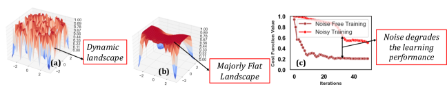
Figure 1: Cost Function Landscapes of 4-qubit QNN (a) With Noise and (b) Without Noise. (c) Comparison of Nosiy and Noise Free Training of 4-qubit QNN. The noise makes the cost function landscape flattened indicating the presence of BPs which eventually hinders the trainability of QNNs.

Various strategies have been proposed to mitigate the effect of BPs [15, 16, 17]. Additionally, the underlying causes of BPs have also been extensively analyzed. Factors such as the type and amount of entanglement [18], expressibility of the QNN[19], and the globality of the cost function [20, 21] and hardware noise [22] have been identified as significant contributors to the occurrence of BPs. Among these, quantum noise stands out as a particularly pivotal factor in the NISQ era. Unlike other sources of BPs, noise is an inherent and inescapable aspect of current quantum technologies, making it critical to address, for enhancing the trainability of QNNs. As the quantum computing field progresses, addressing noise-related challenges in QNNs will be essential for realizing their full potential in practical applications.

I-A Motivational Example

The robustness of QNNs against the noise in NISQ devices is a topic of considerable interest. To further elaborate the fact that noise can induce the BPs in QNNs, potentially constraining their practical utility, in Fig. 1 we show the impact of noise on the cost function landscape, which subsequently influences the training efficacy of QNNs. For the motivational analysis, a 4-qubit QNN is employed, with each qubit undergoing $R_{x}(\theta)$ and $R_{y}(\theta)$ rotation gates. Additionally, controlled-Z (CZ) gate is used to entangle the adjacent qubits. The quantum layers have an overall depth of 10, accounting to a total of 80 single-qubit and 40 two-qubit gates. The qubit measurement is performed in PauliZ measurement basis. The QNN is then trained to learn an identity function, utilizing the Adam optimizer with a learning rate of 0.1 over 50 iterations.

Under ideal, noise-free conditions, the cost function landscape exhibits significant dynamism (Fig. 1a), with multiple regions converging towards a solution. Such a landscape facilitates the optimizer’s navigation towards an optimal solution. Conversely, in the presence of noise, affecting each qubit in every layer, the cost function landscape becomes significantly flatter (Fig. 1b). This flattening renders the landscape less conducive for the optimizer, hampering its ability to locate the solution efficiently. These differences are prominently reflected in training results, where training in the absence of noise yields significantly superior outcomes compared to training under noisy conditions, as shown in Fig. 1c. Therefore, addressing the noise is crucial for the practical realization of scalable QNNs. This paper focuses on a comprehensive analysis of noise, exploring conditions under which noise may be beneficial and strategies to mitigate its impact to a feasible extent.

I-B Our Contributions

We conduct a comprehensive investigation into how quantum noise affects the training dynamics of QNNs. We studied the occurrence of BPs by analyzing training dynamics under noisy and noise-free conditions while keeping quantum layers’ depth constant and increasing the number of qubits. We examined both global (all qubits measured) and local (single qubit measured) cost function definitions. The salient contributions of our paper are summarized below and visually represented in Fig. 2:

• Our analysis shows that quantum noise precipitates the emergence of BPs in QNNs with a global cost function definition, a phenomenon which typically emerges at a relatively higher qubit count in noise-free environments. However, we find that choosing the right qubit measurement observable aligning with the cost function requirements and desired quantum circuit outputs, can significantly mitigate or exploit this effect. To this end we explore various qubit measurement strategies namely; the standard PauliZ, PauliX, PauliY, and a specially designed arbitrary Hermitian observable.

  

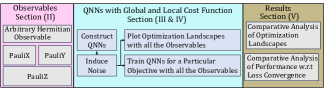
  Figure 2: An Overview of Our Key Contributions.

• In the global cost function setting, we observe that the optimization landscapes for PauliX and PauliY become significantly flatter as the number of qubits increases, a sign of BP emergence, and is more pronounced in noisy environments. PauliZ, however, maintains satisfactory trainability up to 6 qubits and moderate at 8 qubits in noisy conditions, but encounters BPs at 10 qubits.

• A notable finding is that QNNs employing the arbitrary Hermitian observable with a global cost function benefit from noise, resulting in a truncated optimization landscape that eases progression towards the solution. This observable proves effective for training up to 10 qubits, demonstrating that appropriate observable selection can leverage noise to enhance QNN trainability.

• Contrary to the global cost function, the PauliZ observable with a local cost function, shows considerable advantage under noise, maintaining efficient training up to 10 qubits showing the potential of effective training in noisy conditions. Interestingly, there is a minimal influence of the local cost function on the optimization landscapes of PauliX and PauliY observables. The predominantly flat landscapes observed for these observables under both global and local cost functions severely limit their training effectiveness.

Our findings demonstrate that appropriate observable selection can not only mitigate the detrimental effects of noise but also leverage them to enhance the trainability of QNNs.

II Preliminaries

II-A Qubit Measurement and Observables

PauliZ Observable

The PauliZ observable, often represented by the symbol $\sigma_{z}$ or $Z$ is one of the three Pauli matrices used in quantum mechanics. It is particularly significant for its role in describing the state of a qubit, the fundamental unit of quantum information. The PauliZ observable is a $2\times 2$ matrix represented as:

$$\sigma_{z}=Z=\begin{pmatrix}1&0\\ 0&-1\end{pmatrix}$$

This matrix operates on two-dimensional complex Hilbert spaces, which are the state spaces of qubits. In the context of quantum mechanics, the PauliZ observable corresponds to the measurement of spin or polarization along the Z-axis. When applied to a qubit, it differentiates between the two basis states, typically denoted as $\ket{0}$ and $\ket{1}$. The eigenvalues of this matrix are $+1$ and $-1$, corresponding to these basis states. A measurement resulting in +1 indicates the system is in the $\ket{0}$ state, and $-1$ indicates the $\ket{1}$ state.

PauliX Observable

The PauliX observable, denoted by the symbol $\sigma_{x}$ or $X$ is the second Pauli matrix and is represented as:

$$\sigma_{x}=X=\begin{pmatrix}0&1\\ 1&0\end{pmatrix}$$

The Pauli-X observable corresponds to the measurement of spin or polarization along the X-axis. When applied to a quantum state, it effectively flips the state between the two basis states, $\ket{0}$ and $\ket{1}$. The eigenvalues of this matrix are $+1$ and $-1$, corresponding to these flipped states. The PauliX gate is the quantum equivalent of the classical NOT gate. It flips the state of a qubit from $\ket{0}$ to $\ket{1}$ and vice versa, making it fundamental for qubit state manipulation. The eigenstates of the PauliX observable are not the computational basis states ($\ket{0}$ and $\ket{1}$), but rather the superposition states $\frac{\ket{0}+\ket{1}}{\sqrt{2}}$ and $\frac{\ket{0}-\ket{1}}{\sqrt{2}}$. These states are stable under the action of the PauliX observable.

PauliY Observable

The PauliY observable, denoted by the symbol $\sigma_{y}$ or $Y$, is the third Pauli matrix and is represented as:

$$\sigma_{y}=Y=\begin{pmatrix}0&-i\\ i&0\end{pmatrix}$$

In quantum mechanics, the PauliY observable corresponds to the measurement of spin or polarization along the Y-axis. When applied to a quantum state, it provides information about the phase relationship between the basis states $\ket{0}$ and $\ket{1}$. The eigenvalues of this matrix are $+1$ and $-1$, which are related to these phase-adjusted states. It is similar to the X-gate but also introduces a phase shift. The Y-gate, flips the state of a qubit from $\ket{0}$ to $i\ket{1}$ and $\ket{1}$ to $-i\ket{0}$. The eigenstates of the PauliY observable are different from the computational basis states ($\ket{0}$ and $\ket{1}$) and are instead specific superpositions of these states with complex coefficients. These states are stable under the action of the PauliY observable.

Arbitrary Hermitian Observable

A Hermitian observable in quantum mechanics is a fundamental concept that extends beyond the specific examples of the Pauli matrices as discussed above. A Hermitian observable is represented by a Hermitian operator, which is a linear operator $\hat{A}$ on a Hilbert space that equals its own Hermitian conjugate (or adjoint), denoted as $\hat{A}^{\dagger}$. This is mathematically expressed as:

$$\hat{A}=\hat{A}^{\dagger}$$

This means that for any two vectors $\ket{a}$ and $\ket{b}$ in the Hilbert space, the inner product $\bra{a}\hat{A}\ket{b}$ equals the complex conjugate of $\bra{b}\hat{A}\ket{a}$. In quantum mechanics, observables correspond to physical quantities that can be measured, such as position, momentum, spin, etc. The Hermitian nature of these observables ensures that the eigenvalues, which represent the possible outcomes of measurements, are real numbers. This is essential because physical measurements yield real values. The eigenvalues of a Hermitian operator are real, and the eigenvectors corresponding to different eigenvalues are orthogonal. This property is crucial in quantum mechanics, as it allows for the definition of quantum states and the prediction of measurement outcomes.

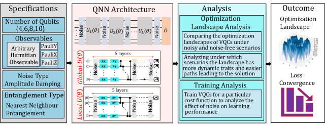
Figure 3: Detailed methodology highlighting key steps for the analysis of noise impact on the trainability of QNNs with different qubit measurement strategies. The quantum circuits used in QNN design are constructed with 4 to 10 qubits. Each qubit has RX and RY gates applied on it, and entanglement was achieved between neighboring qubits via the CZ gate. Two distinct quantum circuit configurations were explored, one where all qubits were measured, and another with only a single qubit measurement. The evaluation metrics used are optimization landscapes and cost function convergence.

II-B Amplitude Damping

Amplitude damping is a concept primarily used in quantum mechanics and refers to a type of quantum noise that causes a quantum system to lose energy. Amplitude damping is a significant concern because it can lead to errors in quantum calculations. It describes how a quantum system, such as a qubit, interacts with its environment, leading to a loss of energy. This interaction can cause changes in the state populations of the qubit, and it is the underlying mechanism behind phenomena such as scattering, dissipation, attenuation, and spontaneous emission.

The mathematical description of the amplitude damping channel is typically provided by Kraus matrices. These matrices are used in quantum mechanics to represent the evolution of quantum states in open quantum systems, i.e., systems that interact with their environment. The amplitude damping channel has two primary Kraus matrices, $A_{0}$ and $A_{1}$, which are defined as follows:

1. $A_{0}$: This matrix describes the probability of the qubit remaining in its current state and is represented as:

   $$A_{0}=\begin{pmatrix}1&0\\ 0&\sqrt{1-\gamma}\end{pmatrix}$$

   where $\gamma$ represents the damping parameter, a real number between 0 and 1, which quantifies the probability of the qubit transitioning from the higher energy state to the lower energy state.

2. $A_{1}$: This matrix represents the transition of the qubit from its higher energy state to its lower energy state due to the interaction with the environment and is described as:

   $$A_{1}=\begin{pmatrix}0&\sqrt{\gamma}\\ 0&0\end{pmatrix}$$

   This matrix captures the essence of amplitude damping: the qubit loses energy, moving from the excited ($\ket{1}$) to ground ($\ket{0}$) state with a probability proportional to $\gamma$.

III HQNET Methodology

In this paper, we investigate the influence of noise on the training dynamics of QNNs. Our analysis primarily utilizes the hardware-efficient ansatz, a popular approach in NISQ applications characterized by sequences of single and two-qubit gates. The general form of these circuits is given by the following Equation:

$$U(\theta)=\prod_{i=1}^{N}U_{\text{ent}}U_{\text{rot}}(\theta_{i})$$ (1)

where $U_{\text{ent}}$ represents a two-qubit gate(s) typically used for qubit entanglement and $U_{\text{\text{rotation}}}(\theta_{i})$ represents a single qubit parameterized gate, whose parameters are optimized during training, and $N$ is the total number of repetitions of the quantum circuit until measurement.

We focus on a comprehensive analysis of the cost function or optimization landscape of QNNs under both noisy and ideal, noise-free scenarios, considering a range of qubit measurement strategies. A key component of our approach involves incrementally increasing the number of qubits, which is crucial for understanding the influence of noise in the context of Barren Plateaus (BP). The concept of BP suggests that the cost function landscape in QNNs tends to flatten with an increase in the number of qubits, thereby posing a significant challenge for optimizers in locating the optimal solution. Moreover, our exploration delves into how different qubit measurement strategies, when applied in noisy conditions, affect the trainability of QNNs. A pivotal aspect of this investigation is to ascertain whether noise can be strategically utilized to enhance the learning process in QNN training. By systematically varying the parameters and conditions, we aim to uncover insights into the role of noise and its potential benefits in the optimization of QNNs. A detailed overview of our methodology is depicted in Fig. 3.

III-A Specifications

We first provide details of the specifications we have used in our QNNs design to carry out the analysis.

Number of Qubits

An important aspect of our study involves examining the trainability of QNNs in relation to the phenomenon of BPs. To comprehensively assess this, we progressively increase the number of qubits. Our investigation starts with QNNs comprising 4 qubits, incrementally increasing in complexity up to QNNs with 10 qubits, i.e., $Q=\{4,6,8,10\}$. This stepwise increase helps in understanding that how the increase in qubit count influences the optimization landscape, particularly in the context of BPs and their impact on trainability under noise and noise-free environments.

Type of Observables

We used different observables for qubit measurement which are PauliZ, PauliX, PauliY and an arbitrary hermitian observable. The details of these observables are already presented in Section II, however, the specific arbitrary hermitian operator that we have used is a specialized observable, constructed as a Hermitian matrix $H$, tailored to the dimensions of the quantum system under investigation. Typically, for a system of $n$ qubits, $H$ is represented by a $2^{n}\times 2^{n}$ matrix, initially populated with zeros in all its elements. A distinct modification is then introduced: the top-left element of $H$ denoted as $H_{0,0}$, is set to 1. This structure transforms $H$ into a high-dimensional analogue of the PauliZ matrix, extending its influence across the entire qubit ensemble. Mathematically, the Hermitian observable that we have used can be described as follows:

$$H=\begin{bmatrix}1&0&\cdots&0\\ 0&0&\cdots&0\\ \vdots&\vdots&\ddots&\vdots\\ 0&0&\cdots&0\end{bmatrix}$$

This corresponds to the projector $\ket{0000}\bra{0000}$, which projects onto the state where all qubits are in the $\ket{0}$ state. This completely aligns with the training goal (cost function) considered in this paper, which is to learn an Identity gate (1 minus the probability of all qubits being in $\ket{0}$ state), details of which are presented later in Section IV.

Type of Noise - Amplitude Damping

Although, there can be different types of noise in NISQ devices which can effect the overall performance of a quantum algorithm. We considered the most common type of noise called as amplitude damping to analyze its impact on the learning performance of QNNs under consideration.

Entanglement Type

Keeping in mind the limitations of NISQ devices, we used the QNNs with nearest neighbor entanglement, i.e., only the adjacent qubits are entangled.

III-B QNN Architecture

Once the required set of specifications are defined, we then contruct the QNNs for our analyis. We contruct two different QNNs differing mainly in the number of qubits measured. In the first QNN, which we call global QNN, we measure all the qubits in the underlying quantum layers. The second is called local QNN, where only a single qubit is measured. We use the hardware-efficient ansatz for quantum layers design, of the form as shown in Equation 1. Below we present the step-by-step details of our methodology:

Global QNN

1. The first step is to define and intialize the qubits. For every qubit number $\in Q$, the qubits are initialized on ground state:

   $$\ket{\psi_{0}}=\ket{0}^{\otimes n}$$

2. Once the qubits are initialized, the next is to apply the unitary transformations. We apply two parameterized gates ($RX$ and $RY$) on each qubit:

   $$U_{rot}=\otimes_{i=1}^{n}RX{(\theta_{i})}RY{(\phi_{i})}$$

   where $\theta_{i}$ and $\phi_{i}$ are the rotation angles for the $i^{th}$ qubit. After the unitray operations, we also entangle the qubits, and as discussed preiously, we use the nearest neighbor entanglement:

   $$U_{entangle}=\prod_{i=1}^{n}CNOT_{i,i+1}$$

   where $CNOT_{i,i+1}$ entangle $i^{th}$ qubit with its neighbor.

3. Given the above gate specifications, the QNN with a single layer is the form:

   $$U=U_{entangle}U_{rot}$$

4. We consider the depth of QNN to be 5, i.e., the above mentioned single layer is repeated 5 times until measurement:

   $$\ket{\psi_{final}}=U^{5}\ket{\psi_{0}}$$

   where the superscript 5 denotes the number of times the layer is repeated. Finally, the qubits are measured to get the output. For an arbitrary Hermitian operator $M$, the probability of measuring a state $\ket{\phi}$ is given by:

   $$P(\phi)=|\bra{\phi}M\ket{\psi_{final}}|^{2}$$

   The Pauli measurements (PauliX, PauliY and PauliZ) are similar to the Hermitian measurement but specifically with Pauli operators as discussed in Section II.

Local QNN

The architecture of local QNN is same as that of global QNN, which is discussed above, however, it differs in terms of qubit measurment, i.e., only a single qubit is measured. For instance, if the $i^{th}$ qubit is measured in PauliZ basis and the outcome is $0$, the post-measurement state of the system can be represented as:

$$\ket{\psi^{\prime}}=\frac{(I\otimes\ldots\otimes\bra{0}_{i}\otimes\ldots\otimes I)\ket{\psi_{final}}}{\sqrt{P(0)}}$$

where, $P(0)$ is the probability of measuring the qubit in state $\ket{0}$, and $\ket{\psi_{final}}$ is the state of the system before measurement and the identity operators $I$ are applied to all qubits except the $i^{th}$ qubit.

III-C Optimization Landscape Analysis

We conduct a detailed analysis of the optimization landscape of the QNNs under investigation. This involves plotting the cost function with respect to the network parameters, creating a landscape through which the optimizer traverses to identify the optimal solution. This analysis typically involves the identification and examination of local and global minima within these landscapes. Landscapes characterized by abundant and broader global minima are generally deemed conducive to effective optimization. Conversely, landscapes predominated by numerous local minima or extensive flat regions are typically considered less favorable for optimization purposes, presenting greater challenges in reaching the optimal solution.

III-D Training Analysis

The QNNs with both local and global cost function definitions are then trained for particular problems. The training analysis encompasses a systematic examination of the convergence behavior of the cost function across a predetermined set of training iterations. This process involves scrutinizing how the cost function evolves and stabilizes during the training phase, thereby providing insights into the effectiveness and efficiency of the learning process over time.

IV Experimental Setup

The QNNs constructed in previous section are subjected to train for learning an Identity function. The cost function this context would be described by the following Equations.

$$C=\bra{\psi(\theta)}(I-\ket{00\ldots 0}\bra{00\ldots 0})\ket{\psi(\theta)}=1-p_{\ket{00\ldots 0}}$$ (2)

We typically want to maximize the probability of all the qubits being in $\ket{0}$ state for global cost function and the probability of first qubit in state $\ket{0}$ for local cost function. This objective closely aligns with the arbitrary Hermitian observable that we have used (See Section III-A) that projects the quantum system to an all $\ket{0}$ state in case of global cost function. For the training analysis, the QNNs are trained for $50$ training iterations. Adam optimizer with a learning rate of $0.1$ is used for the optimization. The experiments are performed using Pennylane [23].

V Results and Discussion

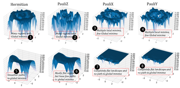
Figure 4: Optimization Landscape of 4-Qubit Global QNN under Noise-Free(upper panel) and Noisy (lower panel) Environments. For all the observables, the landscapes in case of no noise have multiple wider regions containing the solution whereas the landscapes with noise are mostly flat and truncated. For noisy environment, while using the arbitrary Hermitian observable noise can be leveraged to advantage since the landscape trunction provides an easy path to solution.

V-A Global QNN - Comparative Analysis of QNNs Training Dynamics: Noisy vs. Ideal Conditions

We first present a comparative analysis of the training dynamics of QNNs under both ideal (noise-free) and noisy conditions. This analysis focuses on 4 and 6-qubit QNNs, providing insights into the impact of noise on their training efficiency and optimization landscapes. This section aims to explain the distinct challenges and behaviors presented in the presence of noise, and how they differ from ideal, noiseless scenarios. This comparison is vital for understanding the resilience and adaptability of QNNs in real-world applications where noise is an inevitable factor.

V-A1 4-Qubit Global QNN

Optimization Landscape in Noise-Free Setting

In our investigation involving a 4-qubit quantum system, the overall architecture comprises 40 single-qubit gates and 15 two-qubit gates. The analysis of the cost function landscapes, as illustrated in Fig. 4 (upper pannel), reveals distinct characteristics under ideal (noise-free) conditions. In such an environment, all landscapes demonstrate feasibility for optimization regardless of the measurement observable employed. However, a closer examination highlights that landscapes utilizing an arbitrary Hermitian observable and PauliZ measurement observable are particularly more conducive to optimization. These landscapes exhibit multiple wider regions that converge to the solution as shown in label and , indicating a robust optimization potential. In contrast, landscapes associated with PauliX and PauliY measurement observables, while showing similarities to each other, are less optimal from the optimization perspective. They are characterized by limited presence of global minima and an increased presence of local minima, as shown in label and of Fig. 4. Despite this, they still maintain a moderate suitability for optimization, with a somewhat diminished, yet viable, efficiency in reaching the solution.

Figure 5: Training Results of 4-Qubit Global QNN Under Noisy and Noise-Free Environments. The noise-free training is better in all the cases, however, the arbitrary Hermitian observable performs significantly better than other observables in noisy setting.

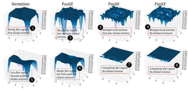
Figure 6: Optimization Landscapes of 6-Qubit Global QNN under Noise-Free (upper panel) Noise free) and Noisy (lower panel) Environments. In case of no noise, the landscapes with arbitrary Hermitian and PauliZ observable seems better as they have few regions containing the global miminum, whereas with PauliX and PauliY observables there are multiple local minima and almost no global minimum. In the presence of noise, PauliX and PauliY observable’s landscapes are completely flat with no room for optimization. The landscape with PauliZ observable is mostly flat with limited training potential. In case of the arbitrary Hermitian observable noise can be leveraged to advantage since the landscape trunction provides an easy path to solution.

Optimization Landscape in Noisy Setting

In scenarios where noise is introduced (Fig. 4(lower pannel), the optimization landscape dynamics alter significantly. The most resilient landscape under these conditions is observed with the Hermitian observable, where a minimal flat region and a broader, smoother trajectory towards the solution are observed, as shown in label in Fig. 4. The PauliZ observable’s landscape, while exhibiting a slightly more flattened region compared to the Hermitian landscape, also maintains a broad and smooth trajectory leading to the solution (label in Fig. 4), and hence is also suitable to optimization. This indicates potential robustness of PauliZ observable against noise.

Conversely, the landscapes corresponding to PauliX and PauliY measurement observables undergo a substantial degradation in the presence of noise. They predominantly display flattened characteristics, with no regions leading to the solution, as shown in label and in Fig. 4. This finding underscores an increased vulnerability to noise for these observables, common in NISQ devices, even in QNNs with shallow quantum layers. In contrast, landscapes associated with Hermitian and PauliZ observables display a significantly dynamic optimization landscape, exhibiting resilience to noise.

Training Comparison in Noisy and Noise-Free Settings

Subsequent training of the 4-qubit QNN, for the problem defined in Equation 2, corroborates these landscape observations (Fig. 4), and the training results are depicted in Fig. 5. Under noise-free conditions, training convergence is achieved across almost all measurement observables. However, in noisy environments, the Hermitian observable demonstrates superior performance with successful convergence. The PauliZ observable, while achieving a degree of training, exhibits suboptimal performance. PauliX and PauliY observables, aligning with their flat cost function landscapes, show negligible learning progress, reflecting their limited efficacy in noisy training scenarios, inevitable in NISQ devices.

V-A2 6-Qubit Global QNN

Optimization Landscape in Noise-Free Setting

In the 6-qubit QNN, comprising 60 single-qubit and 25 two-qubit gates, we observe distinct cost function landscapes for different measurement observables, as shown in Fig. 6(upper panel). Notably, the landscapes becomes more flatter compared to those in the 4-qubit system (Fig. 4), aligning with the BPs definition, which states that an increase in the number of qubits in QNNs leads to a vanishing gradient issue, resulting in progressively flatter landscapes. However, certain observables, notably Hermitian and PauliZ, demonstrate fewer local minima and multiple paths to the global minimum (label and in Fig. 6), offering effective optimization opportunities. Conversely, landscapes involving PauliZ and PauliY observables present multiple local minima with very few or no region containing the solution (label and in Fig. 6), posing a risk of trapping the optimizer in suboptimal solutions.

Figure 7: Training of 6-Qubit Global QNN Under Noisy and Noise-Free Environments. The noise-free training is better with all the observables than noisy training. However, the arbitrary Hermitian observable performs significantly better than other observables and almosy same as in case noise-free training, in noisy setting.

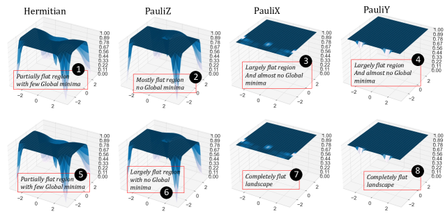
Figure 8: Optimization Landscapes under Noisy Setting for 8-Qubit (upper panel) and 10 Qubit(lower panel) Global QNN. The landscapes for QNNs with more expressive circuits tends to become further flat indicating the occurence of BPs. The landscape for PauliX and PauliY and PauliZ observables are completely and majorly flat with almost no or very limited potential for optimization. The landscape with arbitrary Hermitian observable is starting to get partially flat but still provides a good smoother path to solution.

Optimization Landscape in Noisy Setting

Introducing noise alters the optimization landscapes significantly as shown in Fig. 6(lower pannel). Optimization landscapes associated with PauliX and PauliY observables are the most affected, becoming completely flat offering no room for effective optimization, as shown in label and in Fig. 6. The PauliZ observable also shows a larger flat region in its optimization landscape and absence of the global minimum in the truncated optimization landscape and hence it will be difficult for the optimizer to navigate through to the solution (label in Fig. 6). Interestingly, the arbitrary Hermitian observable’s landscape, while truncated, becomes more conducive to optimization than in the noise-free setting (label in Fig. 6), with a reduced flat region and a wider path to the solution as highlighted in label of Fig. 6).

Training Comparison in Noisy and Noise-Free Settings

The training efficacy of the 6-qubit system, as evaluated for the problem defined in Equation 2 and illustrated in Fig. 7, mirrors the observed landscape dynamics. In the absence of noise, most observables facilitate training, with Hermitian and PauliZ observables demonstrating superior performance, likely due to their landscape characteristics of minimal local minima and multiple global minima. In contrast, under noisy conditions, the Hermitian observable distinctly outperforms others, underscoring its robustness against noise interference.

Since we have already shown how the noise is affecting the peformance in QNNs, from this point onwards, we only present the optimization landscapes and training results for noisy setting.

V-B Global QNN - Focused Analysis QNNs Training Dynamics in Noisy Setting

Building on our established understanding of noise impact on QNN’s performance, subsequent discussions will be centered exclusively on the noisy setting. This narrowed focus will shed light on the ways in which noise alters the optimization terrain in QNNs with more expressive quantum layers (8 and 10 qubits), with different qubit measurement strategies, offering insights into the challenges and potential strategies for achieving effective optimization under realistic, non-ideal conditions.

V-B1 8-Qubit Global QNN

Analysis of Optimization Landscape

The 8-qubit QNN consists of a total of 80 single and 35 two-qubit gates. The optimization landscapes of 8-qubit QNN with different measurement observables are shown in Fig. 8 (upper pannel). We find trends consistent with our previous findings for 4 and 6-qubit QNNs. Specifically, the optimization landscapes for PauliX and PauliY observables are entirely flat, offering no opportunity for convergence to an optimal solution, as shown in label and in Fig. 8. Conversely, the landscape for PauliZ observables, though truncated due to noise, presents some potential for effective training, although with limited regions indicating the presence of a global minimum, as shown in label in Fig. 8, offering potential to somewhat mitigate the negative effects of BPs. Notably, the Hermitian observable demonstrates enhanced robustness in noisy conditions. The truncation in its landscape appears beneficial, providing a smoother and broader path towards the solution, as shown in label of Fig. 8, thus showing a significant potential to alleviate the adverse effects of BP even at higher qubit count.

Training Analysis

The training results of the 8-qubit circuit, as presented in Fig. 9(left), align closely with the observed optimization landscapes. In line with the landscapes, the QNNs with PauliZ and PauliY observables exhibit negligible training progress. In contrast, QNNs using the PauliZ observable show moderate training effectiveness. Most impressively, QNNs employing the Hermitian observable demonstrate robust training performance, approaching optimal solutions and thereby highlighting the noise-resilience of the arbitrary Hermitian observable used in this paper.

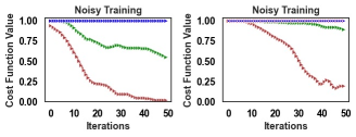
Figure 9: Training of 8 (left) and 10 (right) Qubit Global QNN with Different Observables Under Noise. For both 8 and 10 qubit QNNs, all the Pauli observables show limited or no training performance. Only the arbitrary Hermitian observable performs effective training while benefitting from noise and escaping the BPs.

V-B2 10-Qubit Global QNN

Analysis of Optimization Landscape.

The 10-qubit QNN accounts to a total of 8 100 single and 45 two-qubit gates. In Fig. 8 (lower panel), we present the optimization landscapes associated with QNNs containing 10-qubit quantum layers under various measurement observables. It is observed that landscapes corresponding to PauliX and PauliY observables exhibit a completely flat topology, indicating an absence of optimization opportunities, as shown in label and in Fig. 8. Conversely, the landscape for the PauliZ observable, while predominantly flat, presents marginal optimization potential (label in Fig. 8). Notably, the landscape associated with an arbitrary Hermitian observable is characterized by a truncated and less uniform topology (label in Fig. 8), suggesting a comparatively greater scope for optimization even in 10-qubit QNNs, potentially overcoming the BPs and enhancing the trainability potential of QNNs.

Training Analysis

In Fig. 9(right), we display the training outcomes for the 10-qubit circuit. Consistent with the dynamics observed in the optimization landscape, the model exhibits ineffective training when using any of the three Pauli observables (X, Y, Z). However, when employing the arbitrary Hermitian observable, used in this paper, the model demonstrates effective training performance. This distinction underscores the enhanced suitability of the arbitrary Hermitian observable (defined while keeping in mind the cost function and the output we want from QNN) for training more expressive quantum circuits.

V-C Local QNN: Analysis of QNNs Training Dynamics in Noisy Conditions

In this section, we shift our focus to local QNNs, where only a single qubit is measured. Our previous investigations, detailed in Section V-A, demonstrated that a custom-designed Hermitian observable, well-aligned with our chosen cost function (refer to Section IV), outperformed standard observables (PauliZ, PauliX, and PauliY) in global QNN setup. Thus, this analysis will solely consider these standard observables to evaluate whether localizing the cost function enhances the overall performance of QNNs with these observables. Furthermore, our previous results indicated that in the absence of quantum noise, all observables showed high effectiveness, especially in systems with lower qubit counts (4 and 6 qubits). However, under quantum noise and at higher qubit counts (8 and 10 qubits), these observables encountered barren plateaus (BPs) rapidly. Therefore, this analysis will concentrate on noisy conditions at these larger qubit counts.

V-C1 8-Qubit Local QNN

The optimization landscape of an 8-qubit local QNN employing various observables is depicted in Fig. 10. The results reveals a notable similarity with the optimization landscape observed in global QNN configurations, as illustrated in Fig. 8(upper panel). Specifically, for the PauliX and PauliY observables, the optimization landscape predominantly exhibits flat regions, as shown in label and in Fig. 10 indicating these observables are generally suboptimal for effective optimization irrespective of the cost fucntion globality and locality. In contrast, the optimization landscape associated with the PauliZ observable in the local QNN setting demonstrates a significant divergence from its global QNN counterpart. In QNN with local cost function definition, the landscape for the PauliZ observable is not predominantly flat. Instead, it features multiple expansive regions that encompass the solution, as shown in label of Fig. 10. This characteristic suggests a more favorable scenario for optimization when using the PauliZ observable in QNNs with local cost function definition, in contrast to its behavior in QNNs with global cost function definition where a largely flat landscape is observed (label of Fig. 8 (upper panel)).

This distinction in landscape topology between local and global QNN configurations, particularly with respect to the PauliZ observable, underscores the importance of choosing the appropriate observable in relation to the specific quantum layers architecture being utilized, to enhance the efficiency and success of the optimization process in QNNs.

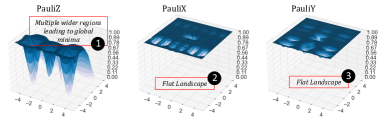
Figure 10: Optimization Landscape of 8-Qubit Local QNN under Noisy Settings with Different Observables. The landscapes with PauliZ observable in local QNN significantly benefits from noise than global QNN as there are multiple wider regions in its landscape leading to solution. PauliX and PauliY observables’ landscape are still completely flat.

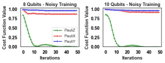
Figure 11: Training Results of 8 and 10 Qubit Local QNN with different observables in Noisy Environment. The landscape with PauliZ observable in local QNN even with 10 qubits still have multiple wider regions leading to the solution. PauliX and PauliY observables’ landscape are still completely flat.

The 8-qubit QNN with local cost function definition with different measurement observables are then subjected to training for the problem defined in Equation 2, the results of which are shown in Fig. 11(left), which typically align with the optimization landscape results in Fig. 10(left). Specifically, the QNNs with PauliX and PauliY observables exhibit negligible or no training progress, in stark contrast to the QNN utilizing the PauliZ observable. Notably, the QNN with the PauliZ observable demonstrates significant training effectiveness, markedly surpassing the performance of the QNNs employing PauliX and PauliY observables.

This comparative analysis highlights the superior adaptability and learning efficiency of local QNN when the PauliZ observable is implemented, as opposed to the limited training efficacy observed with the PauliX and PauliY observables. Such outcomes underline the critical importance of selecting appropriate measurement observables in QNN configurations to achieve optimal training and performance results.

V-C2 10-Qubit Local QNN

The optimization landscapes in case of 10-qubit local QNN with local cost function design, as shown in Fig. 12, do not differ much to that of 8-qubit QNN (with local cost function) design (Fig. 10). The PauliZ observable still exhibits a pretty dynamic landscape with multiple regions containing the solution making it suitable for the optimizers to find the solution, as shown in label of Fig. 12. This shows a greater potential of PauliZ observable when used local cost function definition, to overcome the so called BPs problem even at higher qubit count and under noisy conditions. On the other hand, the optimization landscape for PauliX and PauliY observables are completely flat and are not suitable for the optimization, as shown in label and in Fig. 12 analogous to the case of 8 qubit QNN with local cost function ( and in Fig. 10).

The 10-qubit QNN with local cost function are then trained to learn the problem defined in Equation 2. The training results are typically aligned with their optimization landscape where the PauliZ observable outperforms PauliX and PauliY observables, as shown in Fig. 11(right).

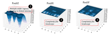
Figure 12: Optimization landscape of 10-Qubit Local QNN with different observables in Noisy Environemnt. The landscapes with PauliZ observable in local QNN still have multiple wider regions leading to solution. PauliX and PauliY observables’ landscape are completely flat.

VI Conclusion

This paper presents a significant contribution to the understanding and enhancement of Quantum Neural Networks (QNNs) training in the presence of quantum noise, a prevalent challenge in the Noisy Intermediate Scale Quantum (NISQ) era. Our findings underscore the pivotal role of quantum noise in precipitating the onset of barren plateaus (BPs), which are known to hinder the scalability and trainability of QNNs. Key insights from our research include the finding that the use of the PauliZ observable in a global cost function setting (all qubit measurement) maintains satisfactory trainability up to 6 qubits, and moderate trainability at 8 qubits, under noisy conditions. However, it also succumbs to BPs at 10 qubits. In contrast, the PauliX and PauliY observables, regardless of the cost function definition, exhibit substantially flatter optimization landscapes with increasing qubit numbers, indicating a quicker onset of BPs in noisy environments.

Our most notable finding is the advantageous use of a custom-designed arbitrary Hermitian observable combined with a global cost function. This approach not only mitigates the detrimental effects of quantum noise but also exploits these noisy conditions to enhance QNN trainability, effectively up to the 10-qubit limit of our study. Furthermore, in a local cost function setting, the PauliZ observable outperforms others, maintaining efficient training capabilities up to 10 qubits.

These results highlight the importance of careful observable selection and cost function definition in QNN training. Our work contributes to the advancement of quantum machine learning research, offering a path forward in optimizing QNNs for real-world applications in the NISQ era.

References

- [1] J. Preskill, “Quantum Computing in the NISQ era and beyond,” Quantum, vol. 2, p. 79, Aug. 2018.
- [2] Z. Liang et al., “Towards advantages of parameterized quantum pulses,” arXiv, no. 2304.09253, 2023.
- [3] Y. Fan et al., “Quantum circuit matrix product state ansatz for large-scale simulations of molecules,” arXiv, no. 2301.06376, 2023.
- [4] J. W. Z. Lau et al., “Nisq computing: where are we and where do we go?,” AAPPS Bulletin, vol. 32, no. 1, p. 27, 2022.
- [5] R. Renner and R. Wolf, “Quantum advantage in cryptography,” AIAA Journal, vol. 61, no. 5, pp. 1895–1910, 2023.
- [6] A. Pyrkov et al., “Quantum computing for near-term applications in generative chemistry and drug discovery,” Drug Discovery Today, p. 103675, 2023.
- [7] D. Herman et al., “Quantum computing for finance,” Nature Reviews Physics, vol. 5, no. 8, pp. 450–465, 2023.
- [8] J. Biamonte et al., “Quantum machine learning,” Nature, vol. 549, pp. 195–202, sep 2017.
- [9] M. Benedetti et al., “Parameterized quantum circuits as machine learning models,” Quantum Science and Technology, vol. 4, p. 043001, nov 2019.
- [10] M. Cerezo et al., “Variational quantum algorithms,” Nature Reviews Physics, vol. 3, no. 9, pp. 625–644, 2021.
- [11] K. Zaman et al., “A survey on quantum machine learning: Current trends, challenges, opportunities, and the road ahead,” 2023.
- [12] E. Farhi and H. Neven, “Classification with quantum neural networks on near term processors,” arXiv, no. 1802.06002, 2018.
- [13] M. Kashif and S. Al-Kuwari, “Design space exploration of hybrid quantum–classical neural networks,” Electronics, vol. 10, no. 23, p. 2980, 2021.
- [14] J. R. McClean et al., “Barren plateaus in quantum neural network training landscapes,” Nature Communications, vol. 9, nov 2018.
- [15] H. Liu et al., “Mitigating barren plateaus with transfer-learning-inspired parameter initializations,” New Journal of Phys, vol. 25, no. 1, p. 013039, 2023.
- [16] M. Kashif and S. Al-Kuwari, “Resqnets: a residual approach for mitigating barren plateaus in quantum neural networks,” EPJ Quantum Technology, vol. 11, no. 1, p. 4, 2024.
- [17] M. Kashif and S. Al-Kuwari, “The impact of cost function globality and locality in hybrid quantum neural networks on nisq devices,” Machine Learning: Science and Technology, vol. 4, p. 015004, jan 2023.
- [18] O. Marrero et al., “Entanglement-induced barren plateaus,” PRX Quantum, vol. 2, p. 040316, Oct 2021.
- [19] M. Kashif and S. Al-Kuwari, “The unified effect of data encoding, ansatz expressibility and entanglement on the trainability of hqnns,” International Journal of Parallel, Emergent and Distributed Systems, vol. 38, no. 5, pp. 362–400, 2023.
- [20] M. Cerezo et al., “Cost function dependent barren plateaus in shallow parametrized quantum circuits,” Nat. Comms, vol. 12, no. 1, 2021.
- [21] M. Kashif et al., “Alleviating barren plateaus in parameterized quantum machine learning circuits: Investigating advanced parameter initialization strategies,” arXiv, no. 2311.13218, 2023.
- [22] S. Wang et al., “Noise-induced barren plateaus in variational quantum algorithms,” Nature Communications, vol. 12, nov 2021.
- [23] V. Bergholm et al., “Pennylane: Automatic differentiation of hybrid quantum-classical computations,” arXiv, 2018.