Parallel-friendly Spatio-Temporal Graph Learning for Photovoltaic Degradation Analysis at Scale

Abstract.

We propose a novel Spatio-Temporal Graph Neural Network empowered trend analysis approach (ST-GTrend) to perform fleet-level performance degradation analysis for Photovoltaic (PV) power networks. PV power stations have become an integral component to the global sustainable energy production landscape. Accurately estimating the performance of PV systems is critical to their feasibility as a power generation technology and as a financial asset. One of the most challenging problems in assessing the Levelized Cost of Energy (LCOE) of a PV system is to understand and estimate the long-term Performance Loss Rate (PLR) for large fleets of PV inverters. ST-GTrend integrates spatio-temporal coherence and graph attention to separate PLR as a long-term “aging” trend from multiple fluctuation terms in the PV input data. To cope with diverse degradation patterns in timeseries, ST-GTrend adopts a paralleled graph autoencoder array to extract aging and fluctuation terms simultaneously. ST-GTrend imposes flatness and smoothness regularization to ensure the disentanglement between aging and fluctuation. To scale the analysis to large PV systems, we also introduce Para-GTrend, a parallel algorithm to accelerate the training and inference of ST-GTrend. We have evaluated ST-GTrend on three large-scale PV datasets, spanning a time period of 10 years. Our results show that ST-GTrend reduces Mean Absolute Percent Error (MAPE) and Euclidean Distances by 34.74% and 33.66% compared to the SOTA methods. Our results demonstrate that Para-GTrend can speed up ST-GTrend by up to 7.92 times. We further verify the generality and effectiveness of ST-GTrend for trend analysis using financial and economic datasets. Our source code, datasets, and a full version of the paper are made available.

1. Introduction

Photovoltaic energy represents a promising solution to growing uncertainty over the stability of the world’s energy resources and lowering the carbon footprint (Gazbour et al., 2018). For large-scale deployment of this well established technology, the financial benefits of investing in commodity scale solar must be highlighted to encourage the adoption of PV power generation. This is best accomplished through careful accounting of all of the possible costs associated with the production of energy. The Levelized Cost of Energy (LCOE) (Darling et al., 2011) is a measurement of the total cost of the generation of one unit of energy, and is used to quantify the profitability of a technology. The LCOE summarizes the lifetime of the system including, initial cost for planning, building, maintenance, and destruction of the site. A significant portion of the LCOE of a PV system is related to its ability to produce the same amount of power under the same weather conditions (Performance Loss) (Jordan et al., 2017b). Performance loss in PV modules on an individual’s roof may impact a single family electricity bill, but the performance loss across fleets PV power plants contribute to millions of dollars in lost revenue. The Performance Loss Rate (PLR) of a photovoltaic (PV) system indicates the decline of the power output over time (in units of % per annum (%/a, or %/year)) (French et al., 2021). PLR represents the physical degradation of PV modules, which is a critical property of any PV system. There are two approximating models to quantify PLR: relative PLR (Lindig et al., 2018), aggregated by comparing power data output to its counterpart from initial state of the PV system and absolute PLR (Ingenhoven et al., 2017), which is the coefficient of the slope of the power output as time goes by.

Figure 1. Example of a PV system with 10-years power timeseries exhibiting non-monotonic degradation pattern.

Nevertheless, traditional PLR estimation typically models PLR as monotonic, linearly decreasing quantities, assuming linear degradation of the system components. In practice, PV degradation can be neither linear nor monotonically decreasing (Hegedus et al., 2000; Jordan et al., 2017b). This leads to erroneous estimation of the performance of PV systems over their lifetimes for methods using aforementioned assumptions (Jordan et al., 2017b). An accurate understanding of the PLR of PV systems is critical to inform the LCOE calculation towards more accurate financial predictions, and allow for targeted assets maintenance  (Deline et al., 2022).

Example 1.1.

Fig. 1 shows example of a ten-years-long timeseries collected from a PV inverter. Observe that in first two years the performance actually goes up and then it degrades in a linear fashion till the end. Hence, we cannot identify a global linear trend to characterize the performance loss rate for this inverter.

We observe that PLR in real PV systems do not always follow a monotonic decreasing or increasing trend. For example, the new installation of PV components may cause a break-in period when the performance of PV systems actually improves (Lindig et al., 2022; Jordan et al., 2017b), then degrades as time goes by, and eventually shows up after the breaking point. Complex phenomena related to module operation can lead to cyclic patterns of power loss and recovery that are both technology and weather dependent. Additionally, transient effects such as the build up of debris on module surfaces can intermittently lower power output (Meyers, 2022).

While several data-driven approaches have been studied for PLR estimation, it remains to be a nontrivial task due to several computational challenges below.

(1) Lack of Large fleet-level Analysis: Traditional PLR Power prediction methods such as 6K, PVUSA, XbX, and XbX+UTC (Huld et al., 2011; King et al., 1997; Curran et al., 2017; Jordan et al., 2017a) can only provide stand-alone PLR analysis for a single PV system, yet does not scale to large-scale, fleet-level PLR analysis (French et al., 2021).

(2) Domain-knowledge Heavy: Conventional PLR estimation methods (Huld et al., 2011; King et al., 1997; Curran et al., 2017; Jordan et al., 2017a) often rely on domain-knowledge based model tuning and ad-hoc decisions. They rely on domain knowledge and manual effort, such as choosing appropriate thresholds, pre-defined filters and physical models. None of these approaches has addressed a streamlined automated PLR estimation pipeline that can “cold-start” without prior domain knowledge of PV timeseries data. This hinders large-scale PV PLR analysis.

(3) Diverse Degradation Patterns: As remarked earlier, PLR degradation pattern can be non-linear and/or non-monotonic (Lindig et al., 2022), which cannot be extracted by degradation profiling approach that assumes the monotonic degradation pattern (Ulanova et al., 2015). A single PLR value may fail to characterize non-linear PV degradation patterns. Degradation patterns of real-world PV systems may exhibit “raise up then down” rather than a monotonic change as time goes by.

(Spatiotemporal) Graph Neural Networks have been applied for non-linear timeseries forecasting, with recent success in PV power predictive analysis, and PV data imputation (Simeunovic et al., 2021; Karimi et al., 2021; Fan et al., 2023). These methods exploit spatio-temporal-topological features to better learn PV fleet-level representations, and have been verified to outperform state-of-the-art predictive methods in PV performance analysis.

The above observations inspire us to consider new PLR estimation paradigms that take advantage of the following intuition. (1) In ideal PV systems without degradation, long-term power timeseries should be stationary, despite of the variations due to weather conditions across different seasons and years; and (2) power timeseries can be decomposed into two major components - a long-term “degradation” trend that represents the changes (“up” and “down”) in PV performance, and one or multiple fluctuation terms that capture the power timeseries seasonalities and noises. We approach PV degradation estimation as an unsupervised regression problem and investigate GNN-basedd trend analysis to effectively captures long-term degradation patterns for large fleets of PV inverters.

Contributions. We make the following contributions.

(1) We propose ST-GTrend, a spatio-temporal graph autoencoder-based method that can effectively capture the degradation patterns in a fleet of PV systems. ST-GTrend adopts paralleled graph autoencoders (one pattern per GAE) to decompose the input into separated trend and a series of different levels of fluctuation patterns and derives degradation from the trend (aging) GAE channel.

(2) We design a unsupervised learning framework that does not need any prior domain-knowledge. We design a novel learning objective to ensure clear disentanglement between aging and fluctuation terms, consisting of three components: (1) Minimizing the reconstruction error between input and sum of aging and multiple fluctuation terms, (2) Ensuring the smoothness of aging term by reducing the noise level, and (3) Imposing the flatness conditions on the fluctuation terms to ensure stationarity of them.

(3) ST-GTrend supports scalable spatiotemporal graph learning and inference for long-term trend analysis. ST-GTrend achieves this through a novel top-down three-level “Think-like” parallelism graph learning algorithm Para-GTrend.

To our knowledge, ST-GTrend is the first work that uses spatio-temporal graph autoencoders to perform fleet-level degradation analysis, addressing non-linear and non-monotonic trend analysis. We have deployed ST-GTrend on the CWRU CRADLE High Performance Cluster (HPC) for monitoring the degradation patterns of real-world PV systems using proprietary PV timeseries data from our PV manufacturer collaborators. This enables us to provide them real-time feedback of the performance of their PV systems.

Related Work. We summarize related work as follows.

Spatiotemporal Graph Neural Networks. Graph Neural Networks (Wu et al., 2020) has been extensively investigated for graph representation learning. Spatio-Temporal graph neural networks (ST-GNNs) are an extension of GNNs that are designed to model the dynamic node inputs while assuming inter dependency between connected nodes (Wu et al., 2020). ST-GNNs capture both spatial and temporal dependencies of graph nodes with e.g., recurrent graph convolutions (Bai et al., 2020; Seo et al., 2018) or attention layers (Yu et al., 2018; Zheng et al., 2020a). The former captures spatiotemporal coherence by filtering inputs and hidden states passed to a recurrent unit using graph convolutions, while the latter learns latent dynamic temporal or spatial dependency through attention mechanisms.

While prior study specifies GNN-based models for short-term time-series prediction (usually with pre-defined historical and predictive windows), not much has been investigated to capitalize ST-GNNs for providing a long-term trend analysis. Existing short-term predictive methods cannot be easily adapted for unsupervised, long-term PLR analysis, especially given non-linearity and non-monotonicity nature of the long-term trends.

Degradation Analysis in Physical Systems. In general, degradation models can be classified into experienced-based approaches, model-based approaches, knowledge-based approaches, and data-driven approaches (Gorjian et al., 2010; Shahraki et al., 2017). Neural Network-based data-driven approaches has become more popular due to their capacity of capturing complex phenomenon without prior knowledge and producing better approximation than traditional regression methods (Gorjian et al., 2010). Previous work (Ulanova et al., 2015) proposes degradation profiling method for a single timeseries from the complex physical system and solve it as an optimization problem by quadratic programming. Albeit it achieves a clear separation between aging and fluctuation parts on a single timeseries, it fails to capture non-monotonic aging pattern due to the monotonic constraint imposed on aging part. In contrast, ST-GTrend leverages rich spatial correlation from a fleet of physical systems to extract degradation patterns for multiple timeseries, from multiple system components at once. Moreover, architecture design that supports effective scaling out with provable guarantees over large fleet level analysis is not addressed by prior work.

2. Preliminary

Table 1. Summary of Notation.

Notation	Description
$G=(V,E,X_{t})$	a series of spatio-temporal graphs
$G_{t}$	snapshot of $G$ at time t
$V$	set of nodes in $G$
$E$	set of edges in $G$
$A$	adjacency matrix of $G$
$X_{t}$	node attributes (timeseries)
$k$	the number of fluctuation terms
$h_{a}$	aging term
$h_{f_{i}}$	$i$-th fluctuation term
$M$	ST-GTrend Model
$P$	set of processors/workers

PV Network Model. We model a large-fleet PV timeseries dataset ${\mathcal{G}}$ = $\{G_{1},\ldots G_{T}\}$ as a sequence of undirected graphs (“snapshots”), where for each snapshot $G_{t}=(V,E,X_{t})$ $(t\in[1,T])$, (1) each node in $V$ denotes a PV system or inverter; (2) $E$ refers to the edge set that links (spatially correlated) PV systems; and (3) $X_{t}\in R^{N\times d}$ denotes the attribute/feature tensor at timestamp $t$, where (a) $N$ refers to the number of nodes in $G_{t}$ at time $t$; and (b) each node carries a $d$-ary tuple that records $d$ (PV) measurements at timestamp $t$.

(1) $$A_{i,j}=\begin{cases}1,i\neq j\text{ and }\exp{(-\frac{dist_{ij}^{2}}{\sigma^{2}})}\geq\epsilon\\ 0\text{ otherwise }\end{cases}$$

The above equation derives the adjacency matrix $A$ of a PV network. By default, ST-GTrend adopts $dist_{ij}$ as Euclidean distance between the locations of PV systems $i$ and $j$. $\sigma$ is standard deviation of all pairwise distances. $\epsilon$ is a threshold to control the network sparsity: the larger, the sparser the network is.

PLR: A Characterization. PLR degradation pattern is defined as the “performance loss” measured by power output of PV systems under the standard test conditions (STC) over time (Kaaya et al., 2020). STC (Makrides et al., 2014) means fixed test conditions with $25\degree C$ cell temperature, $1000W/m^{2}$ plane of module irradiance and AM $1.5G$ spectrum. PV scientists conduct accelerated indoor degradation testing and measure the power output under STC to estimate PLR. Despite the simple computation, indoor testing may not reflect how the PV systems actually degrade in real-world due to the varying environmental factors to which real systems are exposed to. This calls for an automated ML-based approach to estimate PLR of real systems using power output streams. We advocate a modeling of the degradation pattern to be the aging (trend) of the timeseries power output over time, and derive the estimated degradation pattern after filtering out the fluctuation terms that capture seasonalities and noises.

Problem Statement. We model PLR estimation as a regression problem. Given the raw PV power timeseries data from a PV fleet, We train a graph neural networks-based model to minimize the error between the real degradation pattern and estimated degradation pattern, by solving an unsupervised regression problem.

More formally, consider a sequence of historically observed PV network graphs $G=\{G_{1},\ldots,G_{T}\}$, where all graphs consist of the same set of nodes $V$ and share the same adjacency matrix $A$, with varying PV measurements at each node over time, we aim to obtain a St-GNN based model such that it fits the “hidden” PLR pattern by minimizing a loss function that quantifies two types of errors: (a) reconstruction error of the aging and fluctuation terms and (b) additional smoothness and flatness regularization.

3. ST-GTrend Framework

We next introduce ST-GTrend architecture and its components.

Model Architecture. We start with the architecture of ST-GTrend. The model ST-GTrend consists of $k+1$ parallelized array of graph autoencoders (GAEs), which decompose input PV signals into one aging term, and $k$ fluctuation terms. (1) The first module (denoted as $GAE_{1}$) extracts and learn an aging representation $h_{a}$, and (2) each module $GAE_{i}$ ($i\in[2,k+1]$) extracts a distinct fluctuation term.

Justification of design. It is essential for ST-GTrend to learn “disentangled” seasonal-trend representations. (1) Separatedly learned sub-patterns can drastically improve timeseries prediction (Feng et al., 2021). (2) Furthermore, instead of leaning a joint representation for multi-seasonal sub-series, ST-GTrend disentangles  seasonal informational using multiple GAEs: one for a separate fluctuation/seasonal representation. Such design has been shown to be more robust to interventions such as the distribution drift (shifts in distribution of external factors) (Woo et al., 2022). (3) Better still, the arrayed design enable a hybrid parallization scheme to scale the training and inference of ST-GTrend model, as verified in Section 5.

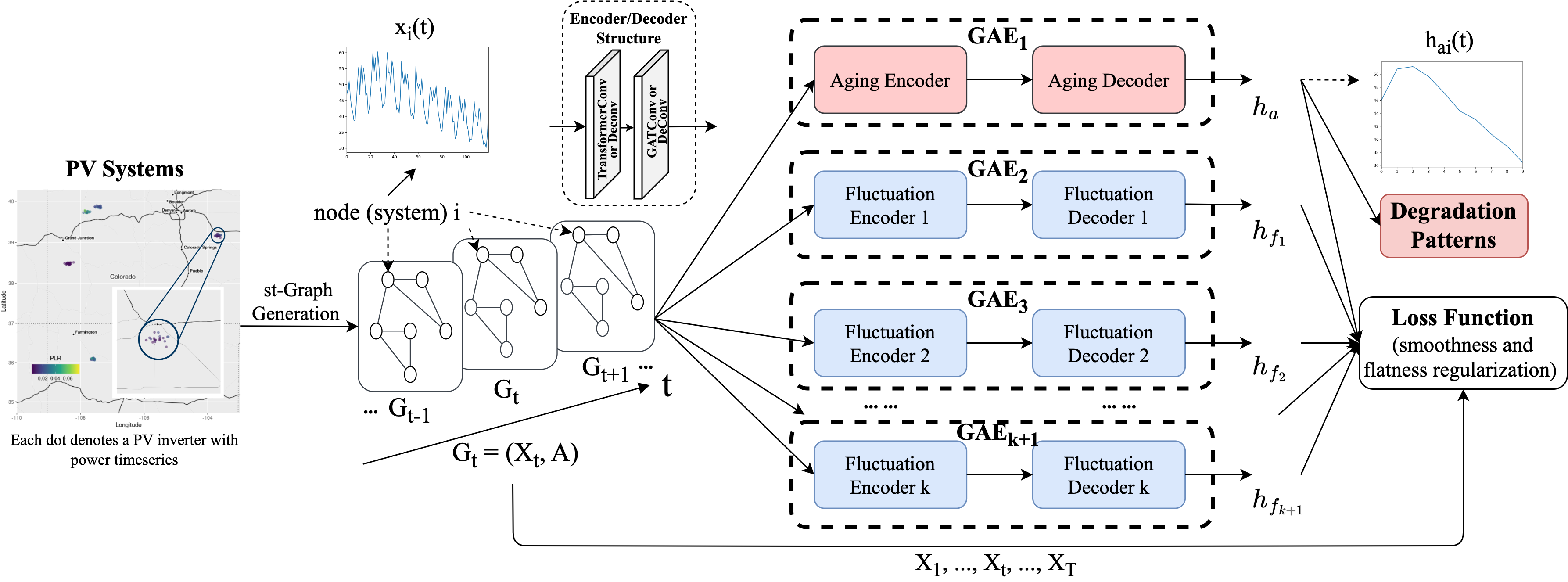
Figure 2. Overview of ST-GTrend Framework (six nodes shown in $G_{t}$ for illustration).

We next specify our design of major components in ST-GTrend.

Parallel GAE Array. As illustrated in Fig. 2, Each GAE module consists of an encoder and decoder. Each encoder or decoder consists of a graph transform operator (TransformerConv or TransformerDeConv) followed by a graph attention operator (GATConv or GATDeConv) to form two convolutional or deconvolutional layers. Both operators leverage attention mechanism. In graph transformer operator, the attention mechanism is applied independently to each node and involves self-attention across nodes. On the other hand, graph attention operator computes attention coefficients using a shared self-attention mechanism across all nodes. This design has its convention from established spatio-temporal GNNs e.g., (Fey and Lenssen, 2019). We adapt such design for basic module in ST-GTrend for aging and fluctuate representations for long-term trend analysis.

Graph Transformer Operators. Graph transformer operators, based on transformer architecture, perform attentive information propagation between nodes by leveraging multi-head attention into graph learning (Shi et al., 2020). Multi-headed attention matrices are adopted to replace the original normalized adjacency matrix as transition matrix for message passing. Therefore, nodes can apply self-attention across nodes and update node representations to effectively aggregate features information from their neighbors. We derive output of timeseries at node $i$ $x^{\prime}_{i}$ as follows:

(2) $$\begin{split}x^{\prime}_{i}&=W_{1}x_{i}+\sum_{j\in N(i)}{\alpha_{i,j}W_{2}x_{j}};\\ \alpha_{i,j}&=\text{softmax}\left(\frac{(W_{3}x_{i})^{T}(W_{4}x_{j})}{\sqrt{D}}\right)\end{split}$$

Here $W_{1},W_{2},W_{3},W_{4}$ are trainable parameters, and $D$ is the hidden size of each attention head .

Spatio-Temporal Graph Attention Operators. We adapt the attention mechanism from graph attention networks (GATs) (Velickovic et al., 2017). The operator uses masked self-attention layers and enable different weights to different nodes in a neighborhood by stacking layers, where nodes are able to attend over their neighborhoods’ features. This makes ST-GTrend more sensitive to useful information from spatial and temporal “neighbors” in the PV networks. We derive the updated representation of timeseries at node $i$ $x^{\prime}_{i}$ as follows:

(3) $$\begin{split}x^{\prime}_{i}&=\sigma\left(\sum_{j\in N(i)}{\alpha_{i,j}Wh_{j}}\right);\\ \alpha_{i,j}&=\frac{\exp(\text{LeakyReLU}(a^{T}[Wh_{i}||Wh_{j}]))}{\sum_{j\in N(i)}{\exp(\text{LeakyReLU}(a^{T}[Wh_{i}||Wh_{j}]))}}\end{split}$$

Here $a$ is the shared learnable attention parameter vector, $W$ is learnable weight matrix, $h_{i}$, $h_{j}$ are input timeseries for nodes i and j, respectively. $\sigma$ is an activation function.

Learning Objective. ST-GTrend introduces rich expressiveness with multiple parallelized GAE array. Meanwhile, a clear disentanglement among GAE outputs should be achieved to distinguish aging and fluctuation representations. We next introduce a novel design of the loss function such that it can achieve a separation between aging and fluctuation for long-term trend analysis for PLR estimation. The loss function consists of reconstruction error, flatness regularization, and smoothness regularization.

Reconstruction Error. We aim to decompose $X$ into aging term $h_{a}$ and $k$ different fluctuation terms $h_{f_{1}},h_{f_{1}},\ldots,h_{f_{k}}$ using $k+1$ GAEs. To ensure the quality of decomposition, we want to minimize the reconstruction error as follows:

(4) $$RE=||X-h_{a}-\sum_{q=1}^{k}h_{f_{q}}||^{2}$$

Flatness Regularization. To ensure stationarity of fluctuation, we propose two constraints on $h_{f}$: (1) mean constraint: we segment every timeseries to ensure difference of mean between each segment within the series being as small as possible and (2) slope constraint: sum of absolute value of global slope of extracted $h_{f}$ for each node should be as close to zero as possible.

For mean constraint (MC), we partition $h_{f}$ of each node into $p$ segments each with length $w$. The length of w determines the temporal resolution of extract fluctuation term. We then minimize the sum of difference between mean values of each pair of the segments to ensure flatness of the fluctuation over time defined as:

(5) $$MC=\sum_{q=1}^{k}\sum_{l=1}^{N}\sum_{i,j=1}^{p}(m_{q_{l_{i}}}-m_{q_{l_{j}}})^{2}W_{ij}$$

Here (1) $m_{q_{l_{i}}}$ denotes the mean of the $i$-th segment of the $l$-th node’s $q$-th fluctuation term, (2) $W$ is a weight matrix, where each entry $W_{ij}$ denotes a learnable weight to minimize the mean difference between segmented pair $m_{l_{i}}$ and $m_{l_{j}}$. To ensure the long-term mean being minimized, we apply linear growth of the weight based on the distance between $m_{l_{i}}$ and $m_{l_{j}}$. This is based on the following intuition: the farther the two segments are from each other, the more weights are given to minimize their mean difference.

Slope Constraint. The slope constraint (SC) ensures the global flatness of each fluctuation level, and is defined as:

(6) $$SC=\sum_{q=1}^{k}\sum_{l=1}^{N}\big{|}slope(h_{f_{q_{l}}})\big{|}$$

Here the slope is calculated from the least square fit.

Smoothness Regularization. We also want to reduce noises in $h_{a}$ by minimizing sum of the standard deviation of the first-order differences of aging term of all the nodes. We thus introduce a smoothness regularization (SR) term as:

(7) $$SR=\sum_{l=1}^{N}SD(h_{a_{l}}[t+1]-h_{a_{l}}[t])$$

where $t\in[1,T-1]$ with $T$ the total number of timestamps, and SD denotes standard deviation.

Loss Function. Putting these together, we formulate the loss function of ST-GTrend as:

(8) $$\mathcal{L}(X,h_{a},h_{f})=RE+\lambda_{1}MC+\lambda_{2}SC+\lambda_{3}SR$$

Here RE, MC, SC, SR are defined in the Eq. 3-6. $\lambda_{1}$, $\lambda_{2}$, and $\lambda_{3}$ control the trade-off between reconstruction error and the quality of disentanglement between aging and fluctuations. The loss function aims to minimize the reconstruction loss while ensuring the flatness of the fluctuation terms and smoothness of the aging term.

PLR Calculation. The output of ST-GTrend can be used to derive both estimated degradation pattern (EDP) and global PLR. $h_{a}$ directly provide the EDP for all systems in the PV fleet. We derive global PLR of system $i$ by calculating the percent of performance loss or gain between any element $v$ in $h_{a_{i}}$ and its corresponding one year apart element $v^{\prime}$ through:

(9) $$PLR_{global}=\frac{1}{m}\sum_{i=1}^{m}\frac{v^{\prime}-v}{v}\times 100\%$$

Where $m$ is the total number of one year apart pairs in $h_{a_{i}}$.

Time-cost Analysis. We present an analysis on the inference cost of ST-GTrend. It takes in total $O(Lmf+LPnf^{2})$ (Gao et al., 2022) to derive decomposed results for a timestamp. Here $n$, $m$, $L$, $P$ and $f$ denote number of nodes, number of edges, number of layers of GAE modules, propagation order of message passing (which is bounded by the diameter of PV network), and dimensions of the node features, respectively. As $L$ and $P$ are often small for practical GAE designs, and $f$ are small constants in real PV data, the overall inference cost (including estimating EDP or global PLR) is $O((Lmf+LPnf^{2})T+nT)$, which is bounded in $O((m+n)T)$.

Algorithm 1 : Para-GTrend

1:Input: A batch of snapshots ${\mathcal{G}}=\{G_{1},\ldots,G_{T}\}$, (optional) ST-GTrend Model $M$, number of fluctuation terms $k$, a set of window sizes $W$, a set of processors $P$, a coordinator processor $P_{0}$, number of epochs $e$;

2:Output: Incrementally trained $M^{\prime}$ upon batch ${\mathcal{G}}$.

3:for $m=1$ to $e$ do

4:     for $i$ in $1$ to $k+1$ do in parallel $\triangleright$ Model Parallelism

5:         if $m=1$ then

6:              $P_{0}$ creates $G_{i}$, a copy of $G$;          

7:         for $j$ in $1$ to $\lceil\frac{T}{W_{i}}\rceil$ do in parallel $\triangleright$ Data Parallelism

8:              if $m=1$ then

9:                  $P_{0}$ ships $G_{i,j}=G_{j+(i-1)\times W_{i}:j+i\times W_{i}}$ to $P_{i,j}$;

10:                  $P_{i,j}$ creates $GAE_{i,j}$;               

11:              $GAE_{i,j}.forward(G_{i,j})$; $\triangleright$ Pipeline Parallelism

12:              Backpropagate and update local gradient of $GAE_{i,j}$;          

13:         if $m=epochs$ then

14:              $GAE_{i}=aggregate(GAE_{i,j}),\forall j\in[1,\lceil\frac{T}{W_{i}}\rceil]$;               

15:$P_{0}$ derives $M^{\prime}$ by assembling all $GAE_{i}$, $\forall i\in[1,k+1];$

16:return $M^{\prime}$ from $P_{0}$;

Figure 3. Para-GTrend: Three-level Parallel Training.

4. Parallelization and Deployment

The design of ST-GTrend is “parallel-friendly” (Ben-Nun and Hoefler, 2019). We next introduce a parallel algorithm, denoted as Para-GTrend, to scale the learning and inference of ST-GTrend to large PV network degradation analysis. Para-GTrend exploits parrallelism with three levels of computation (as illustrated in Fig. 4).

Level I: “Think-like Branch” Model Parallelism. ST-GTrend contains parallelized GAE array with $GAE_{1},\ldots,GAE_{k+1}$ branches, as shown in Fig. 2. $GAE_{1}$ is the aging branch. $GAE_{2},\ldots,GAE_{k+1}$ are the fluctuation branches. This presents opportunities for parallelizing the training by distributing GAE branches among processors. In each training epoch, Para-GTrend computes the forward propagation in parallel without coordination. The output of each branch will be assembled together by an coordinator processor $P_{0}$ to calculate global loss in Eqn. 8. Then each branch backpropagates independently and updates their local gradients in parallel.

Level II: “Think-like Snapshot” Data Parallelism. Within each branch, ST-GTrend takes a sequence of “snapshots” $\{G_{1},\ldots,G_{T}\}$ as the input. Para-GTrend processes the temporal components of the input with a specified length $L$ in parallel. For each fluctuation branch, $L$ is set to be the window size $w$ for the corresponding fluctuation branch. For example, in Fig. 4, there are three fluctuation branches, each with different window size corresponding to “month”, “quarter”, and “year”. For aging branch, $L=\min_{j\in[2,k+1]}w_{j}$. Besides, ST-GTrend exploits the mini-batch data parallelism (MBDP) in DGL (Zheng et al., 2020b) to achieve even larger speed-up. It splits the information propagation of the network into parallelly computed message flow graphs induced by mutually disjoint node batches.

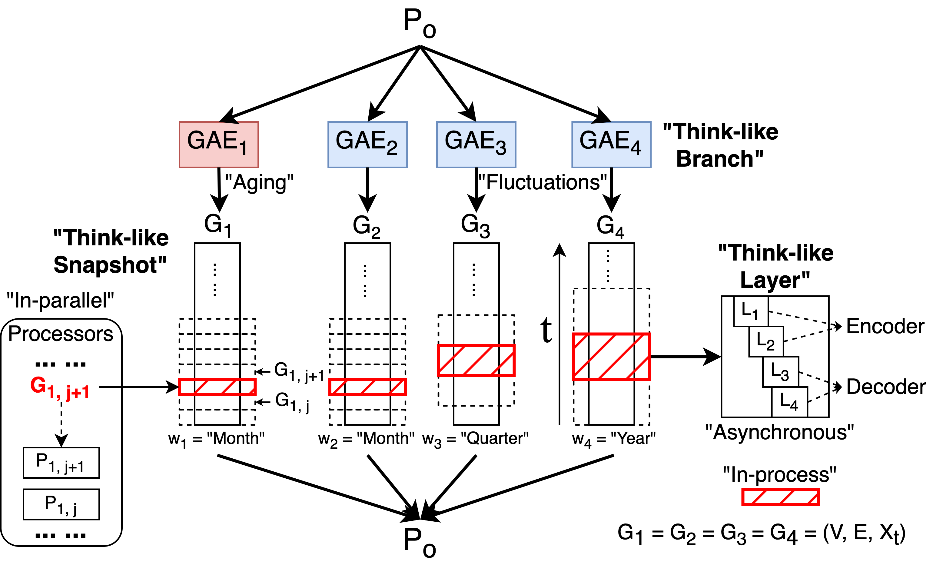
Figure 4. Proposed Para-GTrend ($k=3$ for illustration: one aging channel and three fluctuation channels).

Level III:“Think-like Layer” Pipeline Parallelism. Each branch of ST-GTrend encompasses two layers for encoder, and another two layers for decoder. We adopt an asynchronous macro-pipeline parallelism schema (Narayanan et al., 2019) to parallelize the computation of layers within each GAE, such that inter-layer synchronization is eliminated (without information loss, i.e., the batched graphs from level II are independent of each other). A worker processing its graph batch starts the graph operation on the new layer as soon as it completes the non-linearity in previous layer (Besta and Hoefler, 2022).

To measure the parallelism of Para-GTrend, we extend the notion of parallel scalability (Kumar and Gupta, 1991; Fan et al., 2014) to graph learning.

Definition 4.1.

A training algorithm is parallel scalable if its parallel time cost is inverse proportional to the number of parallel processors, with additional cost that is independent of input size.

Theorem 4.2.

The training algorithm Para-GTrend is scale-free with a total parallel cost in $O\left(\frac{T(G,M)}{\lvert P\rvert}+f(\theta)\right)$ time, where $T(G,M)$ is total cost without parallelism and $f(\theta)$ is independent of the size of $G_{t}$ and linear to the length of timeseries.

Proof Sketch. Given the input G (a series of $G_{t}$) and model M and the total cost of ST-GTrend training without parallelism $T(G,M)$, since the maximum speed-up is bounded by the number of processors/workers utilized, which is $\lvert P\rvert$, the lower bound of the cost of Para-GTrend is $\frac{T(G,M)}{|P|}$. We denote the communication overhead between the coordinator and processors/workers as $f(\theta)$ which is in $O(k\lceil\frac{T}{W_{min}}\rceil e)$, where $w_{min}=\min\{w_{1},w_{2},\ldots,w_{k+1}\}$. Since $w_{min}$ and $k$ are hyper-parameters, $f(\theta)$ is independent of the the number of nodes $|V|$ and number of edges $|E|$. $f(\theta)$ is linear to the length of timeseries $|T|$. Therefore, the total cost of Para-GTrend is in $O\left(\frac{T(G,M)}{\lvert P\rvert}+f(\theta)\right)$ such that $f(\theta)$ is independent of size of the $G_{t}$ and linear to the length of timeseries.

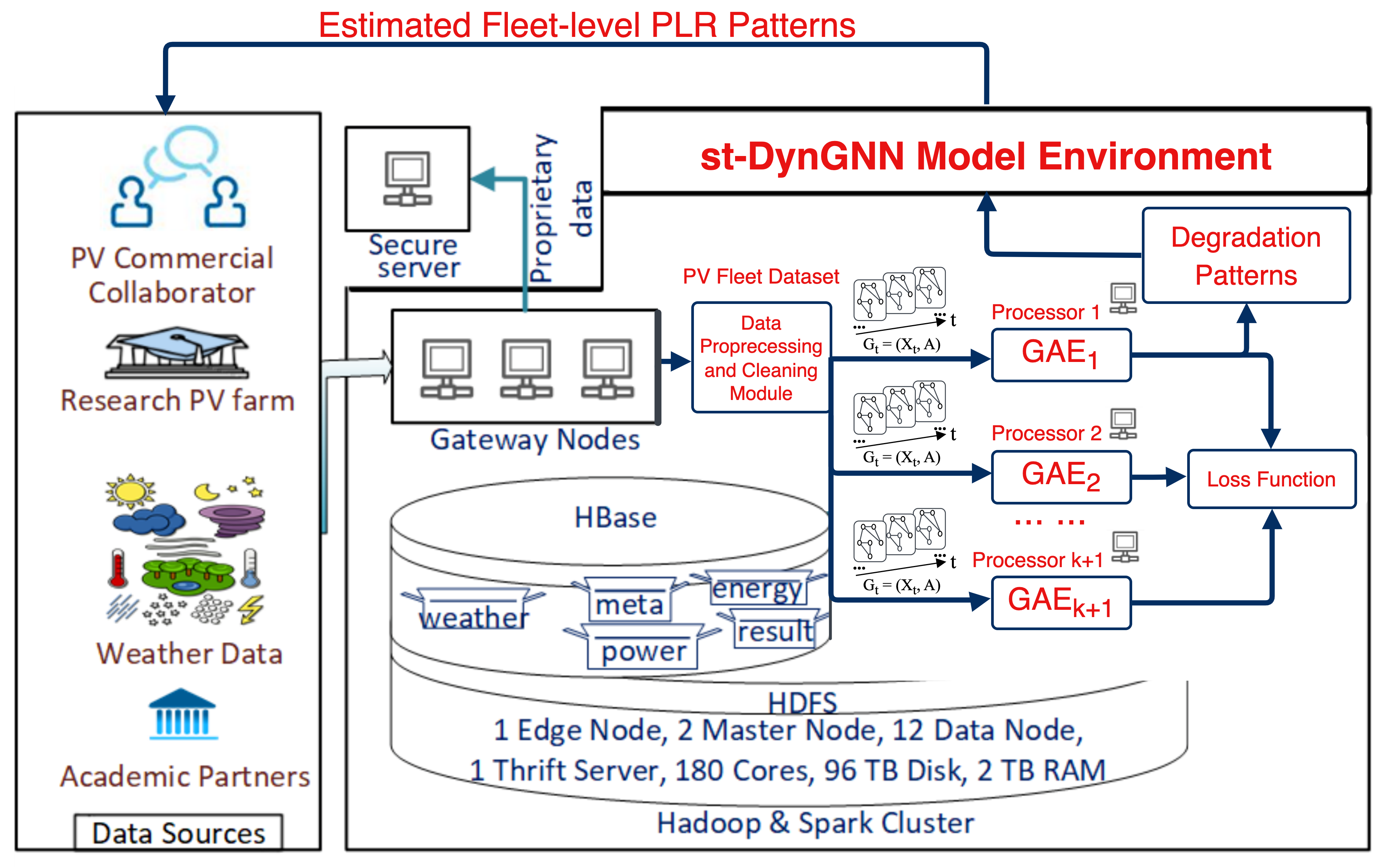
Figure 5. Illustration of ST-GTrend Workflow with Level I Parallelism Implemented for PV Systems from Our Industry Partners (deployed in CRADLE (Nihar et al., 2021)).

System Deployment. ST-GTrend has been deployed to improve PV PLR estimation for commerical plants from SolarEdge (energy company). Fig. 5 illustrates how ST-GTrend (with Level I Model Parallelism illustrated) is incorporated into the our high performance cluster (HPC) CRADLE (Nihar et al., 2021) and communicates with industrial partners. Acquisition of high-quality data is challenging and crucial for PLR degradation analysis on real-world PV systems. Our developed spatio-temporal data imputation python package (Fan et al., 2024) provides high-quality data for ST-GTrend training and inference. ST-GTrend leverages Para-GTrend to accelerate training and inference using computational resources in HPC. The estimated fleet-level PLR results are then forwarded to our PV commercial collaborators and research PV farms. Our proposed framework is generally applicable to other domains that involves spatiotemporal long-term timeseries analysis,e.g., trend analysis in traffic volumes at intersections, air quality changes in urban environments, monitoring the trend of the spread of infectious diseases, and etc. Domain knowledge from corresponding fields can guide the choice of hyperparameters such as the number of fluctuation terms $k$ and corresponding window sizes $w$ needed and trains ST-GTrend accordingly.

5. Experiments

We experimentally verify the performance of ST-GTrend compared with baselines, in terms of accuracy and case analysis of estimated degradation patterns.

5.1. Experimental Setup

Evaluation Metrics. We evaluate the degradation estimation errors using Euclidean Distance (ED) and Mean Absolute Percent Error (MAPE). Smaller values of ED and MAPE indicate better PLR estimations, as they represent a closer match between the EDP (estimated degradation pattern) and RDP (real degradation pattern).

ED. Reporting a single degradation rate for the entire system does not capture the system’s performance dynamics over time. We establish a novel way to quantify how well a model can estimate PLR degradation pattern, consisting of the following two steps: (1) Rescaling: Given RDP and EDP, we rescale every data point in RDP and EDP by dividing them by their respective first values and (2) Error Calculation: We calculate ED between scaled RDP and EDP.

MAPE. We define MAPE as follows:

(10) $$MAPE=\sum_{L=1}^{N}\sum_{J=1}^{T}\frac{|EDP_{L_{J}}-RDP_{L_{J}}|}{N\times T\times|RDP_{L_{J}}|}\times 100\%$$

where $EDP_{L_{J}}$ is the $J-th$ coefficient of EDP for node $L$.

Datasets. We verify our model on five datasets, including three PV datasets and two real-world datasets from Economy and Finance: (1) PV_Case1: It refers to the PV datasets exhibiting global linear degradation patterns. (2) PV_Case2: It refers to the PV datasets showing a piecewise linear degradation pattern with a breakpoint (a change in the degradation rate at the second year). (3) PV_Case3: This refers to the PV dataset exhibiting a non-linear exponential degradation. Each PV dataset consists of 10-year power output timeseris from 100 inverters in 5 PV sites from Colorado, USA. Every power output timeseries includes sample interval of 15 minutes, amounting to 350,592 data points for each PV inverter. Each PV site contains spatially correlated inverters such that inverters in close proximity experience similar degradation severity. Each inverter (PV system) is located in one of the five clusters, each with a $\pm 4\%$ noise in geo-spatial position, and with a $\pm.2\%$ noise.

To demonstrate the generality of ST-GTrend for trend analysis in other applications, we also adopt the following public datasets. (4) Finance : This refers to weekly stock prices of the 500 companies listed in S&P 500 from 12/13/2018 to 12/13/2023. (5) Economy : an annual GDP (in current US dollars) of G20 countries in past 50 years sampled from 1973 to 2022. For finance (resp. economy) data, each node represents a stock (resp. country). For both datasets, we used a thresholded pairwise absolute pearson correlation among node attributes (timeseries) to establish edges.

We obtain the RDP of stock and GDP timeseries using empirical mode decomposition (Huang et al., 1998) which is widely applied in finacial and economic trend analysis (Deng et al., 2022; Dai and Zhu, 2020; Mao et al., 2020; Saâdaoui and Messaoud, 2020). We split each dataset by nodes, 50% for training, 25% for validation, and 25% for testing.

Baselines. We compare ST-GTrend with eight baselines.

(1) 6K (Huld et al., 2011): a domain-specific model, which incorporates irradiance and module temperature as a fraction of standard irradiance and difference from standard temperature.

(2) PVUSA (King et al., 1997): an established physics-based PLR estimation model. The assumption of the model is that the current of a solar panel is a function of the irradiance and the voltage is a function of the irradiance and the module temperature.

(3) XbX (Curran et al., 2017): a data-driven, multiple regression predictive model. The model enables change of point PV degradation pattern modeling.

(4) XbX + UTC (Jordan et al., 2017a): The XbX + UTC is based on the XbX model by introducing a universal temperature correction (UTC) to produce a single temperature coefficient that can be used to convert to the desired representative temperature value.

(5) MSTL (Trull et al., 2022): Multiple Seasonal-Trend Decomposition using Loess (MSTL) decomposes a time series into a: trend component, multiple seasonal components, and a residual component. MSTL uses STL to iteratively extract seasonal components from a time series.

(6) SSA (Apaydin et al., 2021): Singular Spectrum Analysis (SSA) allows extraction of alleged trend, seasonal and noise components from time series. The name comes from singular decomposition of a matrix into its spectrum of eigenvalues. The time series can be reconstructed by regrouping different important components.

(7) QP-Aging-Detect (Ulanova et al., 2015): The QP-Aging-Detect, is a mathematical model using Quadratic Programming (QP) to profile long-term degradation by decomposing timeseries into the aging and fluctuation terms. For fair comparison, we remove the monotonic (strictly increasing or decreasing) constraint imposed on aging component when implementing it in CVXPY (Diamond and Boyd, 2016).

(8) STGAEs: Spatio-Temporal Graph Autoencoders (STGAEs) are variants of ST-GTrend, where the encoder and decoder layers in ST-GTrend are replaced by either Graph Convolutional (GCN) Layers (Kipf and Welling, 2017) for STGAE1 or graph attention layers (Velickovic et al., 2017) for STGAE2.

Hyperparameter Tuning. We use grid search based on the validation loss to identify the optimal set of hyper-parameters (Pontes et al., 2016) for ST-GTrend. We varied the number of fluctuation term $k$ in the set $\{1,2,3,4\}$, network sparsity $\epsilon$ in the set $\{0,0.25,0.5,0.75,1\}$, number of epochs in the set $\{100,250,500,750,1000\}$, learning rate from $\{0.001,0.01,0.05,0.1\}$, regularization terms $\lambda_{1}$, $\lambda_{2}$, and $\lambda_{3}$ all in the set $\{1,5,10,25,50,75,100,200\}$. Based on the validation loss, we choose $k$ equal to 1, $\lambda_{1}$, $\lambda_{2}$, and $\lambda_{3}$ to be 5, 100, and 10 separately, epsilon to be 0.5, epochs to be 500, the learning rate to be 0.05.

Model Training. ST-GTrend is trained by Adam optimizer (Kipf and Welling, 2017) and implemented with PyTorch Geometric Temporal (Rozemberczki et al., 2021), on 12 Intel(R) Xeon(R) Silver 4216 CPU @ 2.10GHz, 128 GB Memeory, 16 cores, and 8 32GB NVIDIA V100 GPU from Case Western Reserve University (CWRU) High Performance Computing (HPC) Cluster.

Table 2. Comparison of Degradation Pattern Estimation Error between ST-GTrend and Baselines. The best-performing results are highlighted in bold, while the second-best ones are italicized. (“ST-GTrend-NF”: ST-GTrend w/o flatness regularization; “ST-GTrend-NS”: ST-GTrend w/o smoothness regularization; “-”: not available due to being PV domain methods).

	Datasets
	PV_Case1		PV_Case2		PV_Case3		Finance		Economy
Models	MAPE	ED	MAPE	ED	MAPE	ED	MAPE	ED	MAPE	ED
6K	11.97 ± 0.71	0.410 ± 0.024	11.11 ± 0.70	0.424 ± 0.025	12.14 ± 0.67	0.410 ± 0.024	-	-	-	-
PVUSA	4.66 ± 0.26	0.167 ± 0.010	4.59 ± 0.26	0.178 ± 0.010	4.71 ± 0.25	0.166 ± 0.010	-	-	-	-
XbX	4.21 ± 0.11	0.147 ± 0.004	4.20 ± 0.10	0.161 ± 0.004	4.18 ± 0.07	0.144 ± 0.003	-	-	-	-
XbX+UTC	1.27 ± 0.04	0.052 ± 0.002	1.22 ± 0.04	0.045 ± 0.002	1.21 ± 0.04	0.044 ± 0.002	-	-	-	-
QP-Aging-Detect	2.38 ± 0.21	0.071 ± 0.005	1.18 ± 0.07	0.043 ± 0.002	2.57 ± 0.24	0.073 ± 0.005	28.16 ± 1.52	2.12 ± 0.12	13.17 ± 0.97	0.45 ± 0.02
MSTL	1.84 ± 0.09	0.055 ± 0.003	1.90 ± 0.10	0.064 ± 0.003	1.45 ± 0.09	0.041 ± 0.003	24.47 ± 1.66	1.94 ± 0.13	10.70 ± 0.73	0.37 ± 0.02
SSA	2.03 ± 0.19	0.059 ± 0.004	1.13 ± 0.08	0.041 ± 0.003	1.96 ± 0.17	0.054 ± 0.004	21.72 ± 1.46	1.70 ± 0.11	17.37 ± 1.07	0.57 ± 0.04
STGAE1	0.61 ± 0.03	0.022 ± 0.002	2.00 ± 0.18	0.071 ± 0.006	2.23 ± 0.19	0.069 ± 0.005	22.12 ± 1.33	1.75 ± 0.11	16.67 ± 1.02	0.58 ± 0.03
STGAE2	0.46 ± 0.02	0.018 ± 0.001	2.04 ± 0.15	0.075 ± 0.005	1.81 ± 0.15	0.053 ± 0.004	21.85 ± 1.31	1.72 ± 0.11	10.53 ± 0.69	0.36 ± 0.01
ST-GTrend-NF	2.84 ± 0.19	0.094 ± 0.005	1.46 ± 0.11	0.052 ± 0.003	2.33 ± 0.14	0.076 ± 0.005	26.69 ± 1.48	2.31 ± 0.13	14.89 ± 0.86	0.51 ± 0.01
ST-GTrend-NS	0.69 ± 0.03	0.027 ± 0.001	1.01 ± 0.04	0.038 ± 0.001	1.95 ± 0.05	0.068 ± 0.001	21.26 ± 1.27	1.68 ± 0.10	9.49 ± 0.65	0.35 ± 0.01
ST-GTrend	0.40 ± 0.02	0.015 ± 0.001	0.96 ± 0.04	0.036 ± 0.001	0.85 ± 0.03	0.031 ± 0.001	18.65 ± 1.15	1.44 ± 0.08	9.31 ± 0.61	0.31 ± 0.01

5.2. Experimental Results

Exp-1: PLR Degradation Estimation Errors. To evaluate the PLR degradation pattern estimation accuracy, we compare MAPE and ED between the RDP and EDP. Table 2 presents PLR degradation pattern estimation errors of ST-GTrend and three types of PV datasets, each exhibiting a different type of degradation pattern: linear, linear with breakpoint, and non-linear and two other datasets from finance and economy.

We observe that ST-GTrend achieves the best PLR degradation pattern estimation measured by MAPE and ED across all datasets. Compared to the top two baselines XbX+UTC and STGAE2, ST-GTrend achieves a reduction of 34.74% and 33.66% on average in MAPE and ED. Moreover, even in the more challenging degradation patterns Case2 and Case3, ST-GTrend continues to outperform the other baselines significantly. These results demonstrate that ST-GTrend models have the potential to provide accurate estimation of PLR degradation patterns for all systems within a large PV fleet.

Exp-2: Detail Evaluations of ST-GTrend. We conduct case studies to validate the quality of disentaglement between aging and fluctuation terms decomposed by ST-GTrend and the effectiveness of the design of encoder an decoder in ST-GTrend.

Decomposition Results from ST-GTrend. Fig. 6 illustrates extracted aging and fluctuation terms of a PV system under linear with breakpoint and non-linear degradation patterns. From this figure, we observe that ST-GTrend achieves a clear disentanglement between aging and fluctuation terms. Aging term successfully captures the initial upward trend in the cases 2 degradation pattern. Fluctuation term captures annual seasonality and noises from the input timeseries. Our results indicate that design of graph autoencoder and learning objective in ST-GTrend is effective in separating aging and fluctuation in PV dataset.

Effectiveness of Encoder and Decoder Design. To further analyze the effectiveness of the encoder and decoder design of ST-GTrend, we quantify the estimation errors changes when replacing the graph convolution layers in ST-GTrend by either graph convolutional (GCN) layers in STGAE1 or graph attention networks (GAT) layers in STGAE2. We observe that STGAE1 and STGAE2 incurs larger PLR estimation errors, on average 89.8% and 65.7% larger MAPE, when compared to ST-GTrend. Our results verify the effectiveness of design of autoencoder in ST-GTrend.

Visual Analysis. We compare EDP extracted by ST-GTrend and top six best-performed baselines with RDP. Fig. 7 shows ST-GTrend can better recover real degradation pattern from input timeseries than all baselines since it show a closer match with RDP. We can see EDP extracted by ST-GTrend is the closest to RDP in both case 2 and case 3 figures followed by XbX+UTC and STGAE2, which is consistent with the comparison of degradation pattern estimation error results shown in Table. 2.

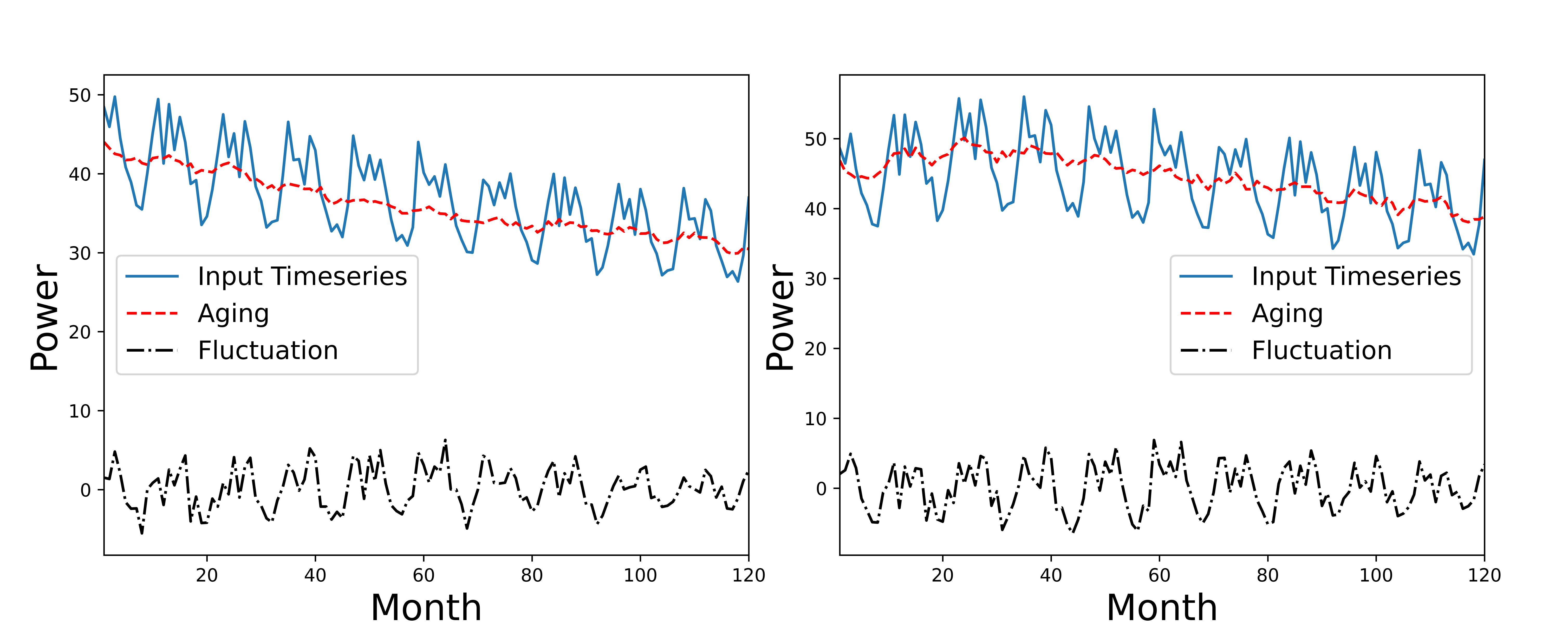
Figure 6. Example of Extracted Aging (in red) and Fluctuation Terms (in black) by ST-GTrend for a PV System (left: PV_Case 3, right: PV_Case 2).

Figure 7. Comparison of Real Degradation/Trend Pattern with Patterns Extracted by ST-GTrend and Baselines (left: PV_Case 2; mid: PV_Case 3; right: Finance).

Exp-3: Ablation Analysis. To study how regularization terms imposed on learning objective impact the accuracy of ST-GTrend, we conduct two ablation analyses to remove the flatness regularization or smoothness regularization from our learning objective in Eq. 8 to study how they affect the accuracy of ST-GTrend. As illustrated in Table. 2, as for the flatness regularization, we find that ST-GTrend with flatness regularization reduces MAPE and ED by 58.10% and 54.92% on average compared to ST-GTrend without flatness regularization (ST-GTrend-NF). On the other hand, for smoothness regularization, we observe that ST-GTrend with smoothness regularization reduces MAPE and ED by 30.87% and 31.27% on average compared to ST-GTrend without smoothness regularization (ST-GTrend-NS). These results verify the effectiveness of regularization terms in the design of ST-GTrend.

(a) Dataset: PV

(b) Dataset: Economy

Figure 8. Scalability Test on Model and Data Parallelism (training time measured by averaging 50 rounds).

Exp-4: Scalability Test. We conduct controlled scalabilty tests on ST-GTrend to report the individual improvement of data or model parallelism alone. (1) We report the scalability of Level I (Model) Parallelism by distributing the training of GAE branches into parallel workers (CPUs). As shown in Fig. 8, the training time (on both PV and Economy datasets) is inverse proportional to the number of workers as it increases from 2 to 8. In other words, the speed-up achieved by model parallelism are proportional (linear) to the number of workers. (2) We next report the result for the Level II (Data Parallelism) where we use multiple workers (GPUs) to train local GAE by fitting the batched input spatio-temporal graph snapshots in parallel. Fig. 8 verifies that Para-GTrend scales well with more computing resources. The training efficiency of ST-GTrend reduces are improved by 7.56 times as the number of workers increases from 2 to 8.

6. Conclusion

We have proposed ST-GTrend, a novel spatiotemporal GNN that adopts paralleled graph autoencoder modules to decompose input photovoltaic (PV) power timeseries into aging (PV performance loss) and fluctuation terms for long-term trend (PLR) analysis. Each module exploits spatial coherence from neighboring PV inverters and temporal correlations within-series to perform aging and fluctuation extractions for PV fleet-level analysis. The loss function of ST-GTrend ensures the clear disentanglement between aging and fluctuation through smoothness and flatness regularizations. To accelerate ST-GTrend training and inference at scale, we have also developed Para-GTrend, a hybrid parallelism algorithm, combining both model and data parallelism to facilitate scalable graph learning. Our experiments have verified that ST-GTrend outperforms existing SOTA methods over PV datasets with diverse degradation patterns and datasets, generalizes to other types of datasets, and scales well with more computing resources.

References

- (1)
- Apaydin et al. (2021) Halit Apaydin, Mohammad Taghi Sattari, Kambiz Falsafian, and Ramendra Prasad. 2021. Artificial intelligence modelling integrated with Singular Spectral analysis and Seasonal-Trend decomposition using Loess approaches for streamflow predictions. Journal of Hydrology 600 (2021), 126506.
- Bai et al. (2020) Lei Bai, Lina Yao, Can Li, Xianzhi Wang, and Can Wang. 2020. Adaptive graph convolutional recurrent network for traffic forecasting. Advances in Neural Information Processing Systems 33 (2020), 17804–17815.
- Ben-Nun and Hoefler (2019) Tal Ben-Nun and Torsten Hoefler. 2019. Demystifying parallel and distributed deep learning: An in-depth concurrency analysis. ACM Computing Surveys (CSUR) 52, 4 (2019), 1–43.
- Besta and Hoefler (2022) Maciej Besta and Torsten Hoefler. 2022. Parallel and distributed graph neural networks: An in-depth concurrency analysis. arXiv preprint arXiv:2205.09702 (2022).
- Curran et al. (2017) Alan J Curran, Yang Hu, Rojiar Haddadian, Jennifer L Braid, David Meakin, Timothy J Peshek, and Roger H French. 2017. Determining the power rate of change of 353 plant inverters time-series data across multiple climate zones, using a month-by-month data science analysis. In 2017 IEEE 44th Photovoltaic Specialist Conference (PVSC). IEEE, 1927–1932.
- Dai and Zhu (2020) Zhifeng Dai and Huan Zhu. 2020. Forecasting stock market returns by combining sum-of-the-parts and ensemble empirical mode decomposition. Applied Economics 52, 21 (2020), 2309–2323.
- Darling et al. (2011) Seth B Darling, Fengqi You, Thomas Veselka, and Alfonso Velosa. 2011. Assumptions and the levelized cost of energy for photovoltaics. Energy & environmental science 4, 9 (2011), 3133–3139.
- Deline et al. (2022) Chris Deline, Mike Deceglie, Dirk Jordan, Matt Muller, Kevin Anderson, Kirsten Perry, Robert White, and Mark Bolinger. 2022. Reducing Uncertainty of Fielded Photovoltaic Performance (Final Technical Report). Technical Report NREL/TP-5K00-82816. National Renewable Energy Lab. (NREL), Golden, CO (United States). https://doi.org/10.2172/1880076
- Deng et al. (2022) Changrui Deng, Yanmei Huang, Najmul Hasan, and Yukun Bao. 2022. Multi-step-ahead stock price index forecasting using long short-term memory model with multivariate empirical mode decomposition. Information Sciences 607 (2022), 297–321.
- Diamond and Boyd (2016) Steven Diamond and Stephen Boyd. 2016. CVXPY: A Python-embedded modeling language for convex optimization. Journal of Machine Learning Research 17, 83 (2016), 1–5.
- Fan et al. (2014) Wenfei Fan, Xin Wang, Yinghui Wu, and Dong Deng. 2014. Distributed graph simulation: Impossibility and possibility. Proceedings of the VLDB Endowment 7, 12 (2014), 1083–1094.
- Fan et al. (2023) Yangxin Fan, Xuanji Yu, Raymond Wieser, David Meakin, Avishai Shaton, Jean-Nicolas Jaubert, Robert Flottemesch, Michael Howell, Jennifer Braid, Laura Bruckman, Roger French, and Yinghui Wu. 2023. Spatio-Temporal Denoising Graph Autoencoders with Data Augmentation for Photovoltaic Data Imputation. Proc. ACM Manag. Data 1, 1, Article 50 (may 2023), 19 pages. https://doi.org/10.1145/3588730
- Fan et al. (2024) Yangxin Fan, Xuanji Yu, Raymond Wieser, Yinghui Wu, and Roger French. 2024. PVplr-stGNN. SDLE Research Center, Case Western Reserve Universitu. https://pypi.org/project/PVplr-stGNN/ PyPI.
- Feng et al. (2021) Jie Feng, Yong Li, Ziqian Lin, Can Rong, Funing Sun, Diansheng Guo, and Depeng Jin. 2021. Context-aware spatial-temporal neural network for citywide crowd flow prediction via modeling long-range spatial dependency. ACM Transactions on Knowledge Discovery from Data (TKDD) 16, 3 (2021), 1–21.
- Fey and Lenssen (2019) Matthias Fey and Jan E. Lenssen. 2019. Fast Graph Representation Learning with PyTorch Geometric. In ICLR Workshop on Representation Learning on Graphs and Manifolds.
- French et al. (2021) Roger H French, Laura S Bruckman, David Moser, EURAC Lindig, Mike van Iseghem, Joshua S Stein, Maurice Richter, Magnus Herz, Wilfried van Sark, Franz Baumgartner, et al. 2021. Assessment of performance loss rate of PV power systems. (2021).
- Gao et al. (2022) Xinyi Gao, Wentao Zhang, Yingxia Shao, Quoc Viet Hung Nguyen, Bin Cui, and Hongzhi Yin. 2022. Efficient Graph Neural Network Inference at Large Scale. arXiv preprint arXiv:2211.00495 (2022).
- Gazbour et al. (2018) Nouha Gazbour, Guillaume Razongles, Elise Monnier, Maryline Joanny, Carole Charbuillet, Françoise Burgun, and Christian Schaeffer. 2018. A path to reduce variability of the environmental footprint results of photovoltaic systems. Journal of cleaner production 197 (2018), 1607–1618.
- Gorjian et al. (2010) Nima Gorjian, Lin Ma, Murthy Mittinty, Prasad Yarlagadda, and Yong Sun. 2010. A review on degradation models in reliability analysis. In Engineering Asset Lifecycle Management: Proceedings of the 4th World Congress on Engineering Asset Management (WCEAM 2009), 28-30 September 2009. Springer, 369–384.
- Hegedus et al. (2000) Steven S Hegedus, Brian E McCandless, and Robert W Birkmire. 2000. Analysis of stress-induced degradation in CdS/CdTe solar cells. In Conference Record of the Twenty-Eighth IEEE Photovoltaic Specialists Conference-2000 (Cat. No. 00CH37036). IEEE, 535–538.
- Huang et al. (1998) Norden E Huang, Zheng Shen, Steven R Long, Manli C Wu, Hsing H Shih, Quanan Zheng, Nai-Chyuan Yen, Chi Chao Tung, and Henry H Liu. 1998. The empirical mode decomposition and the Hilbert spectrum for nonlinear and non-stationary time series analysis. Proceedings of the Royal Society of London. Series A: mathematical, physical and engineering sciences 454, 1971 (1998), 903–995.
- Huld et al. (2011) Thomas Huld, Gabi Friesen, Artur Skoczek, Robert P Kenny, Tony Sample, Michael Field, and Ewan D Dunlop. 2011. A power-rating model for crystalline silicon PV modules. Solar Energy Materials and Solar Cells 95, 12 (2011), 3359–3369.
- Ingenhoven et al. (2017) Philip Ingenhoven, Giorgio Belluardo, and David Moser. 2017. Comparison of statistical and deterministic smoothing methods to reduce the uncertainty of performance loss rate estimates. IEEE Journal of Photovoltaics 8, 1 (2017), 224–232.
- Jordan et al. (2017a) Dirk C Jordan, Chris Deline, Sarah R Kurtz, Gregory M Kimball, and Mike Anderson. 2017a. Robust PV degradation methodology and application. IEEE Journal of photovoltaics 8, 2 (2017), 525–531.
- Jordan et al. (2017b) Dirk C. Jordan, Timothy J. Silverman, Bill Sekulic, and Sarah R. Kurtz. 2017b. PV Degradation Curves: Non-Linearities and Failure Modes. Progress in Photovoltaics: Research and Applications 25, 7 (July 2017), 583–591. https://doi.org/10.1002/pip.2835
- Kaaya et al. (2020) Ismail Kaaya, Sascha Lindig, Karl-Anders Weiss, Alessandro Virtuani, Mariano Sidrach de Cardona Ortin, and David Moser. 2020. Photovoltaic lifetime forecast model based on degradation patterns. Progress in Photovoltaics: Research and Applications 28, 10 (2020), 979–992.
- Karimi et al. (2021) Ahmad Maroof Karimi, Yinghui Wu, Mehmet Koyuturk, and Roger H French. 2021. Spatiotemporal Graph Neural Network for Performance Prediction of Photovoltaic Power Systems. In Proceedings of the AAAI Conference on Artificial Intelligence.
- King et al. (1997) David L King, Jay A Kratochvil, and William E Boyson. 1997. Field experience with a new performance characterization procedure for photovoltaic arrays. Sandia National Lab.(SNL-NM), Albuquerque, NM (United States) (1997).
- Kipf and Welling (2017) Thomas N. Kipf and Max Welling. 2017. Semi-Supervised Classification with Graph Convolutional Networks. In ICLR.
- Kumar and Gupta (1991) Vipin Kumar and Anshul Gupta. 1991. Analysis of scalability of parallel algorithms and architectures: A survey. In Proceedings of the 5th international conference on Supercomputing. 396–405.
- Lindig et al. (2018) Sascha Lindig, Ismail Kaaya, Karl-Anders Weiß, David Moser, and Marko Topic. 2018. Review of statistical and analytical degradation models for photovoltaic modules and systems as well as related improvements. IEEE Journal of Photovoltaics 8, 6 (2018), 1773–1786.
- Lindig et al. (2022) Sascha Lindig, Marios Theristis, and David Moser. 2022. Best practices for photovoltaic performance loss rate calculations. Progress in Energy 4, 2 (2022), 022003.
- Makrides et al. (2014) George Makrides, Bastian Zinsser, Markus Schubert, and George E Georghiou. 2014. Performance loss rate of twelve photovoltaic technologies under field conditions using statistical techniques. Solar Energy 103 (2014), 28–42.
- Mao et al. (2020) Xuegeng Mao, Albert C Yang, Chung-Kang Peng, and Pengjian Shang. 2020. Analysis of economic growth fluctuations based on EEMD and causal decomposition. Physica A: Statistical Mechanics and its Applications 553 (2020), 124661.
- Meyers (2022) Bennet Meyers. 2022. Estimation of Soiling Losses in Unlabeled PV Data. In 2022 IEEE 49th Photovoltaics Specialists Conference (PVSC). 0930–0936. https://doi.org/10.1109/PVSC48317.2022.9938567
- Narayanan et al. (2019) Deepak Narayanan, Aaron Harlap, Amar Phanishayee, Vivek Seshadri, Nikhil R Devanur, Gregory R Ganger, Phillip B Gibbons, and Matei Zaharia. 2019. PipeDream: Generalized pipeline parallelism for DNN training. In Proceedings of the 27th ACM Symposium on Operating Systems Principles. 1–15.
- Nihar et al. (2021) Arafath Nihar, Alan J Curran, Ahmad M Karimi, Jennifer L Braid, Laura S Bruckman, Mehmet Koyutürk, Yinghui Wu, and Roger H French. 2021. Toward findable, accessible, interoperable and reusable (fair) photovoltaic system time series data. In 2021 IEEE 48th Photovoltaic Specialists Conference (PVSC). IEEE, 1701–1706.
- Pontes et al. (2016) Fabrício José Pontes, GF Amorim, Pedro Paulo Balestrassi, AP Paiva, and João Roberto Ferreira. 2016. Design of experiments and focused grid search for neural network parameter optimization. Neurocomputing 186 (2016), 22–34.
- Rozemberczki et al. (2021) Benedek Rozemberczki, Paul Scherer, Yixuan He, George Panagopoulos, Alexander Riedel, Maria Astefanoaei, Oliver Kiss, Ferenc Beres, Guzman Lopez, Nicolas Collignon, and Rik Sarkar. 2021. PyTorch Geometric Temporal: Spatiotemporal Signal Processing with Neural Machine Learning Models. In Proceedings of the 30th ACM International Conference on Information and Knowledge Management.
- Saâdaoui and Messaoud (2020) Foued Saâdaoui and Othman Ben Messaoud. 2020. Multiscaled neural autoregressive distributed lag: A new empirical mode decomposition model for nonlinear time series forecasting. International Journal of Neural Systems 30, 08 (2020), 2050039.
- Seo et al. (2018) Youngjoo Seo, Michaël Defferrard, Pierre Vandergheynst, and Xavier Bresson. 2018. Structured sequence modeling with graph convolutional recurrent networks. In International Conference on Neural Information Processing. Springer, 362–373.
- Shahraki et al. (2017) Ameneh Forouzandeh Shahraki, Om Parkash Yadav, and Haitao Liao. 2017. A review on degradation modelling and its engineering applications. International Journal of Performability Engineering 13, 3 (2017), 299.
- Shi et al. (2020) Yunsheng Shi, Zhengjie Huang, Shikun Feng, Hui Zhong, Wenjin Wang, and Yu Sun. 2020. Masked label prediction: Unified message passing model for semi-supervised classification. arXiv preprint arXiv:2009.03509 (2020).
- Simeunovic et al. (2021) Jelena Simeunovic, Baptiste Schubnel, Pierre-Jean Alet, and Rafael E. Carrillo. 2021. Spatio-temporal graph neural networks for multi-site PV power forecasting. CoRR abs/2107.13875 (2021). arXiv:2107.13875 https://arxiv.org/abs/2107.13875
- Trull et al. (2022) Oscar Trull, J Carlos García-Díaz, and Angel Peiró-Signes. 2022. Multiple seasonal STL decomposition with discrete-interval moving seasonalities. Appl. Math. Comput. 433 (2022), 127398.
- Ulanova et al. (2015) Liudmila Ulanova, Tan Yan, Haifeng Chen, Guofei Jiang, Eamonn Keogh, and Kai Zhang. 2015. Efficient long-term degradation profiling in time series for complex physical systems. In Proceedings of the 21th ACM SIGKDD International Conference on Knowledge Discovery and Data Mining. 2167–2176.
- Velickovic et al. (2017) Petar Velickovic, Guillem Cucurull, Arantxa Casanova, Adriana Romero, Pietro Lio, Yoshua Bengio, et al. 2017. Graph attention networks. stat 1050, 20 (2017), 10–48550.
- Woo et al. (2022) Gerald Woo, Chenghao Liu, Doyen Sahoo, Akshat Kumar, and Steven Hoi. 2022. CoST: Contrastive Learning of Disentangled Seasonal-Trend Representations for Time Series Forecasting. In International Conference on Learning Representations.
- Wu et al. (2020) Zonghan Wu, Shirui Pan, Fengwen Chen, Guodong Long, Chengqi Zhang, and S Yu Philip. 2020. A comprehensive survey on graph neural networks. IEEE transactions on neural networks and learning systems 32, 1 (2020), 4–24.
- Yu et al. (2018) Bing Yu, Haoteng Yin, and Zhanxing Zhu. 2018. Spatio-Temporal Graph Convolutional Networks: A Deep Learning Framework for Traffic Forecasting. In Proceedings of the 27th International Joint Conference on Artificial Intelligence. 3634–3640.
- Zheng et al. (2020a) Chuanpan Zheng, Xiaoliang Fan, Cheng Wang, and Jianzhong Qi. 2020a. Gman: A graph multi-attention network for traffic prediction. In Proceedings of the AAAI Conference on Artificial Intelligence, Vol. 34. 1234–1241.
- Zheng et al. (2020b) Da Zheng, Chao Ma, Minjie Wang, Jinjing Zhou, Qidong Su, Xiang Song, Quan Gan, Zheng Zhang, and George Karypis. 2020b. Distdgl: distributed graph neural network training for billion-scale graphs. In 2020 IEEE/ACM 10th Workshop on Irregular Applications: Architectures and Algorithms (IA3). IEEE, 36–44.