The First SRG/eROSITA All-Sky Survey

The first SRG/eROSITA All-Sky Survey (eRASS1) provides the largest intracluster medium-selected galaxy cluster and group catalog covering the western galactic hemisphere. Compared to samples selected purely on X-ray extent, the sample purity can be enhanced by identifying cluster candidates using optical and near-infrared data from the DESI Legacy Imaging Surveys. Using the red-sequence-based cluster finder eROMaPPer, we measure individual photometric properties (redshift $z_{\lambda}$, richness $\lambda$, optical center, and BCG position) for 12,000 eRASS1 clusters over a sky area of 13,116 deg², augmented by 247 cases identified by matching the candidates with known clusters from the literature. The median redshift of the identified eRASS1 sample is $z=0.31$, with 10% of the clusters at $z>0.72$. The photometric redshifts have an accuracy of $\delta z/(1+z)\lesssim 0.005$ for $0.05<z<0.9$. Spectroscopic cluster properties (redshift $z_{\rm spec}$ and velocity dispersion $\sigma$) are measured a posteriori for a subsample of 3,210 and 1,499 eRASS1 clusters, respectively, using an extensive compilation of spectroscopic redshifts of galaxies from the literature. We infer that the primary eRASS1 sample has a purity of 86% and optical completeness ¿95% for $z>0.05$. For these and further quality assessments of the eRASS1 identified catalog, we apply our identification method to a collection of galaxy cluster catalogs in the literature, as well as blindly on the full Legacy Surveys covering 24,069 deg². Using a combination of these cluster samples, we investigate the velocity dispersion-richness relation, finding that it scales with richness as $\log(\lambda_{\rm norm})=2.401\times\log(\sigma)-5.074$ with an intrinsic scatter of $\delta_{\rm in}=0.10\pm 0.01$ dex. The primary product of our work is the identified eRASS1 cluster catalog with high purity and a well-defined X-ray selection process, opening the path for precise cosmological analyses presented in companion papers.

1 Introduction

In the last decades, two outstanding cosmological questions have been raised. What is the nature of dark matter? What drives the accelerated expansion in the late-time Universe? These puzzles can be addressed using observations of the large-scale structure (LSS). There exist two sets of LSS-based cosmological observables (e.g., see the reviews from Weinberg et al. 2013; Will 2014; Ishak 2019). The first set is connected to the homogeneous cosmological background. These probes use standard rulers such as baryon acoustic oscillations and are sensitive to the geometry and the expansion history of the Universe. The second and complementary set of observables relates to the inhomogeneous universe and how the large-scale structure has grown with time: cluster counts, redshift-space distortions in galaxy clustering, and cosmic shear. The growth of the structures in the cosmic web is mainly related to the cosmological model through the $n$-point statistical functions of the dark matter halos (halo mass function, power spectrum, bi-spectrum, etc.). Provided that the cluster scaling relation or the galaxy bias function is under control, one can constrain a set of cosmological parameters from the cluster number counts or the galaxy clustering. Currently, the largest samples of intra-cluster medium (ICM) selected clusters of galaxies considered in cosmological analysis are in the regime of few hundreds (Vikhlinin et al. 2009a, b; Pacaud et al. 2016, 2018; Planck Collaboration et al. 2016a; Zubeldia & Challinor 2019; de Haan et al. 2016; Bocquet et al. 2019). Their constraint on the cosmological model alone is not stringent and depends strongly on the calibration of the mass-observable relation.

eROSITA, on board the Spektrum Roentgen Gamma (SRG) orbital observatory launched in 2019, is a sensitive, wide-field X-ray telescope which has performed an all-sky survey of unprecedented depth (Merloni et al. 2012; Predehl et al. 2021). The sensitivity of eROSITA extends to 10 keV on the high end, but is at its highest in the soft X-ray band, specifically in the 0.2-2.3 keV range, which makes it particularly suitable for detecting and studying emission from the hot gas in galaxy clusters. eROSITA is now delivering an outstanding sample of all the most massive clusters up to redshift $z=1.32$ (Bulbul et al. A&A subm., and this analysis) to constrain cosmological parameters with percent-level precision (Ghiradini et al. A&A subm.) using a mass observable relation calibrated using weak gravitational lensing (Grandis et al. A&A subm.; Kleinebreil et al. A&A subm.; Pacaud in prep.).

To make the most of the unprecedentedly large X-ray-selected galaxy cluster sample provided by eROSITA, it is vital to measure accurately the redshifts of the galaxy clusters. Measuring redshifts based on X-ray data is only possible from the emission lines found in the X-ray spectra of the ICM (e.g., Hashimoto et al. 2004; Lamer et al. 2008; Lloyd-Davies et al. 2011; Yu et al. 2011). For eROSITA, this venue is available only for a small subset of the clusters and at a relatively low precision ($\sim$10%) (Borm et al. 2014). Indeed, since the redshift precision depends strongly on the ICM gas temperature and signal-to-noise ratio of the X-ray spectra, precise measurements are only feasible for very bright clusters observed with long exposure times (e.g., at the ecliptic poles of the eRASS1).

Galaxy clusters contain over-densities of early-type galaxies relative to the field (Dressler 1980). Up to date, the most accurate and precise cluster redshifts are obtained from an ensemble of galaxy redshifts (e.g., Beers et al. 1990; Böhringer et al. 2004; Clerc et al. 2016; Ider Chitham et al. 2020) measured via optical spectroscopy (e.g., Szokoly et al. 2004; Koulouridis et al. 2016; Clerc et al. 2020). Dedicated spectroscopic observations of the galaxies in eROSITA clusters are ongoing with the SDSS-V (Kollmeier et al. 2017) and soon to be started with 4MOST (Finoguenov et al. 2019), so that by 2029 (planned end of 4MOST) essentially all eROSITA clusters will have measured spectroscopic redshifts. Until then, we estimate photometric redshifts using multi-band photometric data to sample the spectral energy distribution of the sources of interest (e.g., review from Salvato et al. 2009). The performance of photometric redshift techniques depends on the quality of the photometry, how well the desired spectral features are sampled by the subset of the spectrum encompassed by the photometric filters, the robustness of the calibration methods, and how representative the spectroscopic training datasets are. Estimating the cluster photometric redshift consists of two steps: identifying cluster-bound galaxies in the optical and infrared data and estimating their redshift via ensemble averaging. Optical cluster finding algorithms are classified by their methodology: matched-filter based algorithms (e.g., Postman et al. 1996; Olsen et al. 2007; Szabo et al. 2011), Voronoi tessellation methods (e.g., Ramella et al. 2001; Soares-Santos et al. 2011; Murphy et al. 2012), friends-of-friends (e.g., Wen et al. 2012) and percolation algorithms (e.g., Dalton et al. 1997; Rykoff et al. 2014). Photometric redshift estimation methods are classified by the information they use: red sequence (e.g., Gladders & Yee 2000; Gladders et al. 2007; Oguri 2014), color overdensities (e.g., Miller et al. 2005), brightest cluster galaxies (BCG) (e.g., Koester et al. 2007; Hao et al. 2010), photometric redshifts of all galaxies (e.g., Wen et al. 2012; Tempel et al. 2018; Bellagamba et al. 2018; Aguena et al. 2021), or spectroscopic galaxy surveys (e.g., Duarte & Mamon 2015; Old et al. 2015).

In this analysis, we consider a sample of candidate clusters detected as extended X-ray sources in the first eROSITA all-sky survey (eRASS1, Merloni et al. 2024; Bulbul et al. A&A subm.). We measure each cluster’s photometric redshift and optical richness following the method of Rykoff et al. (2014). The basis for these measurements is the optical and near-infrared inference models of the extra-galactic sky published in the 9th and 10th data release of the DESI Legacy Imaging Surveys (Dey et al. 2019). It covers almost all the extragalactic sky with a footprint extending over 24,069 deg². In the event of sufficient coverage with galaxy spectra, we measure the cluster spectroscopic redshift and cluster line-of-sight-velocity dispersion using the method from Clerc et al. (2020) and Kirkpatrick et al. (2021).

The article is organized as follows. In Section 2, we introduce the optical and X-ray data. Section 3 describes the optical cluster finding method and defines how the different redshift types are measured. Our main result, the eRASS1 identified cluster and group catalog, is presented in Section 4. We evaluate its properties in the following sections. With the help of consistently reanalyzed catalogs of known clusters, we estimate the completeness of the eRASS1 catalog in Section 5. In Section 6, we compute cluster number densities and examine their dependence on the optical survey depth. We discuss the purity and the properties of the remaining contaminants in the eRASS1 catalog in Section 7. The accuracy and precision of the photometric redshifts are quantified in Section 8. Finally, in Section 9, we combine all cluster catalogs to tightly constrain the richness–velocity dispersion relation and measure its intrinsic scatter. Our results are summarized in Section 10.

Throughout the paper, we assume a flat cosmology with $H_{0}=70$ km s^-1 Mpc^-1, $\Omega_{\rm m}=0.3$, and $\sigma_{8}=0.8$. Redshifts are given in the heliocentric reference frame. No corrections for Virgo infall or the CMB dipole moment have been applied.

2 X-ray, Optical, and Near-infrared Data

In this section, we introduce the data considered in the X-ray wavelength domain (Sec. 2.1) and in the optical and near-infrared range (Sec. 2.2). The observed X-ray radiation of galaxy clusters stems from thermal bremsstrahlung and line emission by the hot Intra-Cluster Medium (ICM). In the optical and near-infrared, old stellar populations emit most of the received light. The different wavelengths thus trace distinct parts of the galaxy clusters.

2.1 The X-ray eRASS1 Cluster Catalog

Galaxy cluster candidates are selected from the first eROSITA All-Sky Survey catalog (eRASS1, Merloni et al. 2024). It consists of X-ray sources in half of the sky at galactic longitude $179.9442\degr<l<359.9442\degr$. Galaxy clusters emit X-ray radiation from their diffuse hot gas. They appear as extended sources in the eROSITA observations as opposed to point sources such as Active Galactic Nuclei (AGNs) or stars, although there can be misclassifications. Therefore, we consider extended eRASS1 sources as galaxy cluster candidates. This sample is described in detail in Bulbul et al. (A&A subm.) and forms the basis for the eRASS1 cluster candidate catalog.

The survey area of eROSITA used here is that to which the German consortium holds data rights and covers half the sky: 20,626 deg² (see Figure 1). The joint coverage of this with the LS (see Section 2.2) is 13,178 deg², primarily because the LS avoids the area around the Galactic plane and the Magellanic clouds. As described in Bulbul et al. (A&A subm.), we further mask regions of known non-cluster extended X-ray sources (using the flag IN_XGOOD=False), in total 62 deg². This reduces the eRASS1 cluster candidate catalog area to 13,116 deg².

A fraction of the extended sources are cataloged multiple times. Most of these split sources are removed by applying the SPLIT_CLEANED flag (Bulbul et al. A&A subm.). In total, the eRASS1 cluster candidate catalog contains 14,818 cleaned sources in the common region between eROSITA_DE and the Legacy Surveys. Figure 1 shows the sky density of cleaned galaxy cluster candidates. The deeper exposures towards the ecliptic poles cause the gradient of source density. This is the main cluster catalog analyzed in the article. Other cluster catalogs analyzed are presented in Section 5.

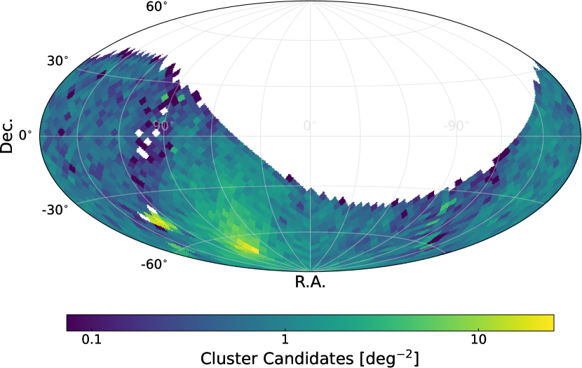
Figure 1: Pixelized number density of 22,718 cleaned eRASS1 extended sources, that is, cluster candidates. The HEALPix map has a resolution of ${\rm NSIDE}=16\leavevmode\nobreak\ \hat{=}\leavevmode\nobreak\ 13.4$ deg². The highest number density occurs near the southern ecliptic pole around $\rm{R.A.}=90\degr$ and $\rm{Dec.}\approx-67\degr$ where the exposure time is largest. Another overdensity of extended sources near the galactic plane around $\rm{R.A.}\approx 135\degr$ and $\rm{Dec.}\approx-45\degr$ is associated with the Vela supernova remnant. It lies outside the common footprint with the Legacy Survey (see Figure 2).

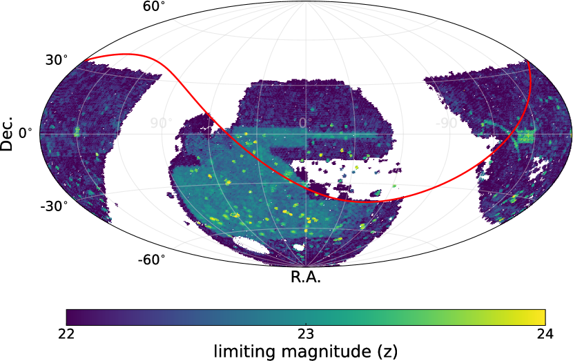
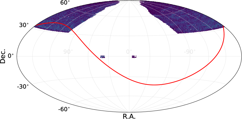
Figure 2: Maps of the limiting magnitude in the $z$ band for sources detected with 10$\sigma$ significance. The footprint maps show the coverage for the Legacy Surveys DR10 south (top panel) and DR9 north (bottom panel). Only regions that have data in all of the $g$-, $r$-, and $z$-bands are considered. The half sky that is covered by eRASS1 corresponds to the region below the red line. The limiting magnitudes in the $z$ band directly translate to the limiting redshift $z_{\rm{vlim}}$ (see Appendix B for details).

2.2 DESI Legacy Imaging Surveys, 9th and 10th Releases

We combine the optical and near-infrared inference model data from the 9th and 10th release of the DESI Legacy Imaging Surveys (LS, Dey et al. 2019) to obtain the largest coverage of the extragalactic sky (Galactic latitude $|b|\gtrsim 20\degr$). The galactic plane is not covered by the observations and thereby excluded from our analysis. Observations at optical wavelengths were carried out with three different telescopes as described in Sections 2.2.1 and 2.2.2. Consequently, the survey area is split at a declination of $\approx$32.375$\degr$. We refer to the southern part as LS DR10 South and the northern part as LS DR9 North.

To increase the wavelength coverage, the LS utilizes 7 years (LS DR10) or 6 years (LS DR9) of infrared imaging data from the Near-Earth Object Wide-field Infrared Survey Explorer (NEOWISE, Lang 2014; Mainzer et al. 2014; Meisner et al. 2017a, b). The limitation of blended sources due to the much lower spatial resolution in the NEOWISE data ($\approx 6\arcsec$) compared to the LS data ($\lesssim 1\arcsec$) is partly overcome by applying forced photometry on the unblurred unWISE maps (Lang 2014) at the locations of the sources that are detected in the LS. Including the 3.4$\mu$m $W1$ band in our analysis allows us to extend the galaxy cluster samples to higher redshift ($z\gtrsim 0.8$).

Photometry is measured consistently for all surveys using The Tractor algorithm (Lang et al. 2016) based on seeing-convolved PSF, de Vaucouleurs, exponential disk, or composite de Vaucouleurs + exponential disk models. All magnitudes are given in the AB system and are corrected for Galactic extinction using the maps from Schlegel et al. (1998) with updated extinction coefficients for the DECam.

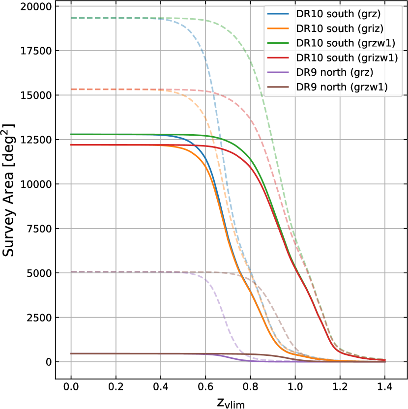
Figure 3: Effective survey area for the Legacy Surveys DR10 south and DR9 north depending on redshift. At the limiting redshift $z_{\rm vlim}$, the faintest considered cluster member galaxy is observed with 10$\sigma$ confidence in the $z$ band. Details are given in Appendix B. The luminosity of that galaxy is $L=0.2$ L_∗ for the eROMaPPer runs which use the $grz$ and $griz$ filter bands and $L=0.4$ L_∗ for the runs that also include the $w1$ band. The dashed lines correspond to the full LS footprint while the continuous lines show the area that is reduced to the overlapping region with eRASS1 (see Figure 2).

2.2.1 LS DR10 south

The catalogs were obtained by processing CTIO/DECam observations (Flaugher et al. 2015) from the DECam Legacy Survey (DECaLS, Dey et al. 2019), the Dark Energy Survey (DES, The Dark Energy Survey Collaboration 2005; Dark Energy Survey Collaboration et al. 2016), and publicly released DECam imaging (NOIRLab Archive) from other projects, including the DECam eROSITA survey (DeROSITAs; PI: A. Zenteno). In the DES area ($\sim 5000$ deg²), the depth reached is higher than elsewhere in the footprint, see Figure 2.

The LS DR10 south covers 19,342 deg² in the $g$, $r$, and $z$-bands (see also Figure 3). When the $i$-band is included, the survey area is 15,326 deg². The overlap with eRASS1 is 12,791 (12,205) deg² when the $i$-band is excluded (included). We describe the calculation of the survey area in Appendix B.

2.2.2 LS DR9 north

In the north (Decl. ¿ 32.375$\degr$), LS uses the Beijing-Arizona Sky Survey (BASS, Zou et al. 2017) for $g$- and $r$-band coverage, and The Mayall $z$-band Legacy Survey (MzLS, Silva et al. 2016) for the $z$-band coverage. Since no additional observations were obtained between DR9 and DR10, the inference catalogs for this part of the sky are that of DR9. It covers 5,068 deg² (see Figure 2). The overlap with eRASS1 is 462 deg².

2.2.3 Processing of released catalogues

We process the LS DR10 south and LS DR9 north data independently because the filter responses of the DECam differ from those of the cameras used by the MzLS and BASS. Fortunately, there is a common area of 341 deg² between the two survey parts, which we use to perform consistency checks (see Section 4.1.2).

Each source in the LS has MASKBITS and FITBITS flags. They encode possible issues encountered in the data (mask) or during the catalog inference process (fit). We discard sources that have set any of the MASKBITS=[0,1,4,7,10,11,12,13] when FITBITS!=9. This mainly affects regions around bright and medium bright stars, around bright galaxies in the Siena Galaxy Atlas (Moustakas et al. 2023), and around globular clusters. The bright galaxies in the Siena Galaxy Atlas are kept even when the listed MASKBITS are set.

2.3 Spectroscopic Galaxy Redshift Compilation

We have compiled 4,882,137 spectroscopic galaxy redshifts from the literature. This compilation serves two goals: calibrating the red-sequence models (Appendix C; $\sim$90,000 redshifts) and calculating spectroscopic cluster redshifts and velocity dispersions. The references considered to create the compilation are listed in Appendix D. There, we list the selection criteria applied to the published catalogs to retrieve high-quality redshifts and to avoid stars or quasi-stellar objects. Dedicated spectroscopic follow-up programs are being undertaken for eRASS1 clusters. We include 154 unpublished galaxy redshifts from Balzer et al. (in prep), who utilize the VIRUS instrument (Hill et al. 2021) on the Hobby-Eberly Telescope (Ramsey et al. 1998; Hill et al. 2021).

All galaxies in the spectroscopic compilation are matched to sources in the LS catalogs using a search radius of 1$\arcsec$. If multiple redshifts are available for a source, we choose the redshift from the closest match.

3 Measurement of Cluster Candidate Counterparts in the Optical and Near-infrared

Star formation in galaxies is quickly quenched after the galaxy reaches the first peri-center on its orbit in the cluster (e.g., Oman & Hudson 2016; Lotz et al. 2019). Optical and near-infrared colors of quenched galaxies are relatively insensitive to stellar ages older than a few Gyrs (e.g., Bruzual & Charlot 2003). Hence, cluster members can be identified by relatively uniform optical and near-infrared colors. These colors strongly depend on redshift, enabling the measurement of photometric cluster redshifts. We identify an X-ray extended source (cluster candidate) as a genuine galaxy cluster by associating it with a coincident overdensity of red-sequence galaxies. The reliability of the identification depends on several factors that we investigate and quantify in the following sections.

We introduce the cluster finder redMaPPer in Section 3.1 and our enhancements to it in the following subsections. We refer to the enhanced redMaPPer package as eROMaPPer.

3.1 redMaPPer

We apply the well-tested and publicly available red-sequence Matched-filter Probabilistic Percolation cluster finder (redMaPPer , Rykoff et al. 2012, 2014, 2016). Its usage is flexible and multi-purpose (e.g., Rykoff et al. 2012; Rozo & Rykoff 2014; Rykoff et al. 2016; Bleem et al. 2020; Finoguenov et al. 2020). The redMaPPer algorithm applies three filters in luminosity, color, and sky position. It finds clusters and creates samples thereof. Spectroscopic verification demonstrates the high purity of the cluster samples obtained: $\gtrsim 90\%$ of the redMaPPer-identified systems are condensations in redshift space, even at the lowest values of optical richness in the HectoMAP redshift survey down to $r=21.3$ (Sohn et al. 2018b, 2020b). Further tests by reshuffling members of true clusters and re-detecting those clusters confirm a high purity of $\gtrsim 95\%$ in the SDSS when $z\in[0.1,0.6)$ (Rykoff et al. 2014), meaning these clusters are not significantly affected by projection effects. In this paper, we define purity as the probability that an extended eRASS1 X-ray source that was optically identified using eROMaPPer is neither an X-ray background fluctuation nor an AGN. The completeness of the returned samples has been estimated for a similar red-sequence-based cluster finder (RedGOLD, Licitra et al. 2016a, b) to be $\sim$100% ($\sim$70%) at $z<0.6$ ($z<1.0$) for galaxy clusters with $M>10^{14}$ M_⊙ (Euclid Collaboration et al. 2019). The decreasing completeness at high redshift relative to results from other cluster finders like AMICO (Bellagamba et al. 2018) is likely attributed to the increasing fraction of blue star-forming galaxies (Nishizawa et al. 2018) to which redMaPPer is insensitive.

Many spectroscopic observing campaigns use a target selection based on redMaPPer catalogs (e.g., Clerc et al. 2016; Rykoff et al. 2016; Rines et al. 2018; Sohn et al. 2018b; Clerc et al. 2020; Kirkpatrick et al. 2021). It has also been used for numerous cosmological experiments (e.g., Costanzi et al. 2019b; Kirby et al. 2019; Ider Chitham et al. 2020; Costanzi et al. 2021), as well as mass calibration analyses (e.g., Saro et al. 2015; Baxter et al. 2016; Farahi et al. 2016; Melchior et al. 2017; Jimeno et al. 2018; Murata et al. 2018; Capasso et al. 2019; McClintock et al. 2019; Palmese et al. 2020; Raghunathan et al. 2019). The impact of projection effects (e.g., Costanzi et al. 2019a; Myles et al. 2020), centering (e.g., Rozo & Rykoff 2014; Hoshino et al. 2015; Hikage et al. 2018; Hollowood et al. 2019; Zhang et al. 2019) and intrinsic alignment (Huang et al. 2018) have also been studied in detail.

redMaPPer can be configured in several different modes, two of which will be used in this paper. When configured in blind (cluster-finding) mode, only the optical and near-infrared galaxy catalogs from the LS are used to identify clusters. When configured in scanning mode, redMaPPer also considers a positional prior from an input cluster catalog. The search radius for cluster members around the fixed input coordinates is equivalent to the cluster radius $R_{\lambda}$ (see Equation (4) in Rykoff et al. 2014)

$$R_{\lambda}=1.0h^{-1}\,{\rm Mpc}\leavevmode\nobreak\ (\lambda/100)^{0.2}.$$ (1)

To identify a cluster at a fixed location, redMaPPer evaluates a likelihood function $\mathcal{L_{\lambda}}$ on a redshift grid (see Equation (76) in Rykoff et al. 2014):

$$\ln\mathcal{L}_{\lambda}=-\frac{\lambda}{S}-\sum_{i}\ln(1-p_{{\rm mem},i}),$$ (2)

where $\lambda$ denotes the optical richness (see Equation (3). The likelihood depends only on the membership probabilities $p_{\rm mem}$, which in turn depend on the color distance from the red-sequence model in all considered filter bands, galaxy luminosity, galaxy spatial distribution, and global background galaxy density (Rykoff et al. 2014, 2016). The richness $\lambda$ is defined as the sum of the membership probabilities multiplied by a scaling factor $S$, which depends amongst other properties on the masked fraction (see Section 11 and Rykoff et al. 2014):

$$\lambda=S\cdot\sum_{i}p_{{\rm mem},i}.$$ (3)

The masked fraction of a cluster is calculated from the number of sources inside $R_{\lambda}$ with nonzero MASKBITS and FITBITS (see Section 2.2) over the total number of sources within $R_{\lambda}$. Using simulations, it was estimated that the richness errors quoted in the redMaPPer catalogs underestimate the observational uncertainties by $\sim$40–70% due to observational noise in the membership probabilities (Costanzi et al. 2019a). A cluster with richness $\lambda=20$ has a typical signal-to-noise ratio of 3.

In the case of a free cluster center (redMaPPer blind mode), a centering likelihood is logarithmically added to $\ln\mathcal{L_{\lambda}}(z)$. The maximum $\ln\mathcal{L}_{\rm max}$ of the resulting likelihood $\ln\mathcal{L}(z)$ is determined, and the corresponding redshift is taken as the photometric cluster redshift $z_{\lambda}$. All other optical cluster properties are evaluated at this redshift.

A minimum of two initial member galaxies is required to start the algorithm. A richness cut of $\lambda>3$ is applied at a later stage.

Enhancements to redMaPPer

First, we promote redMaPPer to a strongly parallel application using the pyspark programming interface. This makes it feasible to run in blind mode on the full LS DR9 and DR10 galaxy catalogs (almost all of the extra-galactic sky) within a few days. Second, we adopt the spectroscopic post-processing from SPIDERS (Clerc et al. 2020; Kirkpatrick et al. 2021); see Section 3.3. Finally, we write a module to select and rank targets for dedicated spectroscopic follow-up programs from SDSS-V (BHM-clusters) and 4MOST (S5). In the following sections, the package encapsulating these features will be referred to as eROMaPPer.

3.2 Cluster Counterpart Association, Photometric Redshift, and Richness Measurements

The optical cluster-finding process and the determination of the cluster optical properties (photometric redshift, richness, etc.) are simultaneous and interdependent. This can result in three distinct outcomes.

3.2.1 Cases with a Single Optical Cluster Counterpart

We determine the photometric cluster redshift, denoted $z_{\lambda}$, by the maximum value of a parabola that is fitted to the $\mathcal{L_{\lambda}}(z)$ curve. It is close to the highest peak of the blue curve in Figure 4, bottom-right panel. The likelihood includes via the membership probabilities the color distance to our red-sequence model, which is described in Appendix C. We analyze the accuracy and precision of the photometric redshifts in Section 8.

3.2.2 Ambiguous Cases with Multiple Optical Clusters along the Line of Sight

We identify ambiguous cases with multiple distinct peaks in $\ln\mathcal{L}(z)$. These correspond to multiple red-sequence overdensities that overlap along the line of sight without necessarily being physically connected. We define the two Gaussians as distinct if their peaks are farther apart than $|z_{\lambda,1}-z_{\lambda,2}|>0.05$, the logarithmic peak ratio is at least $\ln\mathcal{L}(z_{\lambda,2})/\ln\mathcal{L}(z_{\lambda,1})>0.2$, and both cluster likelihoods are above $\ln\mathcal{L}(z_{\lambda,i})>10$ (which roughly corresponds to a richness $\lambda>14$). In this consideration, $z_{\lambda,1}$ is the redshift for the peak of the Gaussian that is closest to the photometric cluster redshift $z_{\lambda}$, and $z_{\lambda,2}$ is the redshift for the peak of the secondary Gaussian.

3.2.3 Cases with no Optical Cluster Counterpart

Cluster candidates (extended X-ray sources) are considered unidentified by eROMaPPer if 1) it is unable to identify at least two red-sequence galaxies at any redshift, 2) the richness of the cluster is $\lambda<3$, or 3) the cluster candidate is sufficiently far outside of the LS footprint. Clusters near the edge of the footprint can still be detected when the circle with radius $R_{\lambda}$ partly overlaps with the footprint. More information for these cases is given in Appendix A.4.

3.3 Spectroscopic Cluster Redshifts

Spectroscopic cluster redshifts $z_{\rm spec}$ provide $\sim$10 times more accurate estimates of the true cluster redshifts compared to our photometric redshifts ($z_{\lambda}$; see Section 8). They are on the other hand more expensive to obtain in terms of telescope time and, therefore, are currently only available for a subset of the clusters. Moreover, they provide a means to estimate the bias and uncertainties of the photometric redshifts (see Section 8) and allow us to calculate cluster velocity dispersions $\sigma$.

The automated algorithm to obtain the spectroscopic cluster redshifts has been adapted from the work of Clerc et al. (2016) and Ferragamo et al. (2020) and is the basis of the automatic spectroscopic redshift pipeline used within the SPIDERS cluster program (Ider Chitham et al. 2020; Clerc et al. 2020; Kirkpatrick et al. 2021). The algorithm is iterative, with the subscript $k$ referring to the $k^{\rm th}$ iteration of the procedure.

First, we match the cluster members, which were selected by eROMaPPer, to our spectroscopic galaxy compilation (see Section 2.3). The number of matches is $N_{\rm spec,0}$. Figure 4, bottom panel, shows the member redshift distribution for the example cluster 1eRASS J085401.2+290316 by the gray bars. The initial spectroscopic cluster redshift is estimated by the bi-weight location estimate (Beers et al. 1990)

$$z_{\rm bwt}=\hat{z}+\frac{\sum_{|u_{j}|<1}\ (z_{j}-\hat{z})[1-u_{j}^{2}(z,z_{j},6)]^{2}}{\sum_{|u_{j}|<1}\ [1-u_{j}^{2}(z,z_{j},6)]^{2}},$$ (4)

where $z$ is a vector of galaxy redshifts, $\hat{z}$ is the sample median, $j$ is the index of the spectroscopic member galaxy and $u_{j}$ is given by

$$u_{j}(z,z_{j},a)=\frac{(z_{j}-\hat{z})}{a\times{\rm MAD}(z)}.$$ (5)

Here, $a=6$ is the tuning constant that regulates the weighting and corresponds to the clipping threshold in units of the median absolute deviation ${\rm MAD}(z)$ of the member galaxy redshifts.

The proper line-of-sight velocity offset (Danese et al. 1980) of all member galaxies is then computed relative to the estimate of the cluster redshift;

$$\frac{v_{j}}{c}=\frac{z_{j}-z_{\rm bwt}}{1+z_{\rm bwt}}.$$ (6)

Figure 4, bottom panel, illustrates for the example cluster 1eRASS J041610.3-240351 the necessity to clip outliers. While the bulk of member redshifts is concentrated around $z=0.40$, ten photometrically selected member galaxies have significantly lower or higher redshifts. Therefore, we perform an initial velocity clipping of members with $|v_{j}|>5,000$ km s^-1 to reject them from the spectroscopic sample of member galaxies. This results in $N_{\rm spec,1}$ spectroscopic members for the first iteration ($k=1$), which are used to recompute the bi-weight cluster redshift using Equation (4). This procedure is iterated until $N_{\rm spec,k}$ converges or a maximum of $k=20$ iterations is reached. In each iteration $k>1$, the clipping velocity is recalculated as $v_{j}>3\sigma_{k}$, where $\sigma_{k}$ is the cluster velocity dispersion for the $k$-th iteration (see Section 3.6). There are several possible outcomes of the clipping procedure:

1. $N_{\rm spec,1}=0$: the initial $5,000$ km s^-1 clipping rejected all members: the procedure cannot proceed and a flag is issued to indicate that convergence failed. This can occur for true systems when several distinct structures along the line of sight are far apart in redshift space.

2. $0<N_{{\rm spec},k}<3$: There is an insufficient number of spectroscopic members left after $k$ steps: it is not possible to estimate the bi-weight redshift estimate (Equation (4)) or the velocity dispersion (Equation (8)) and a flag is issued accordingly.

3. $N_{{\rm spec},k}\geq 3$: the process successfully converges, and the cluster redshift and velocity dispersion are estimated.

In the last case, the remaining objects are called spectroscopic members. Even when the iterative procedure converges, it is essential to check the final clipping velocity. If it is larger than the initial $5,000$ km s^-1, there is likely a substructure that biases the spectroscopic cluster redshift. A flag is assigned in this case. The spectroscopic cluster redshift $z_{\rm spec}$ is calculated by taking the mean of all $z_{\rm bwt}$ values, calculated after bootstrapping the clipped spectroscopic member redshifts 64 times. The standard deviation of these $z_{\rm bwt}$ values is adopted as the spectroscopic cluster redshift uncertainty $\delta z_{\rm spec}$.

In cases 1) and 2), it can still be possible to assign a spectroscopic redshift to a cluster. If there is a spectroscopic redshift available for the identified central galaxy (CG), it is taken as the cluster redshift $z_{\rm spec,cg}$. The uncertainty of the CG redshift is used as the cluster redshift uncertainty. This underestimates the cluster redshift uncertainty because the central galaxy can have a non-negligible line-of-sight velocity with respect to the cluster as a whole (Lauer et al. 2014). We quantify this effect for the eRASS1 clusters in Section 4.2.2. For an example cluster in Figure 4, we mark $z_{\rm spec,cg}$ by the green line. The darker blue line shows the confidence interval $\delta z_{\rm spec}$ of the more robust $z_{\rm spec}$.

3.4 Literature Cluster Redshifts

Survey	Source
ABELL	Andernach (1991)
ACTDR5	Hilton et al. (2020)
CODEX	Finoguenov et al. (2020)
eFEDS	Liu et al. (2022)
GALWEIGHT	Abdullah et al. (2020)
GOGREEN-GCLASS	Balogh et al. (2020)
KIM-HIGHZ-LENSING	Kim et al. (2021)
LP15	Aguado-Barahona et al. (2019)
MADCOWS	Gonzalez et al. (2019)
MARD-Y3	Klein et al. (2019)
MCXC	Piffaretti et al. (2011)
NEURALENS	Huang et al. (2021)
NORAS	Böhringer et al. (2017)
PSZ1	Planck Collaboration et al. (2015)
PSZ2	Planck Collaboration et al. (2016b)
REDMAPPER-DES-SVA	Rykoff et al. (2016)
REDMAPPER-DESY1	McClintock et al. (2018)
REDMAPPER-SDSS-DR8	Rykoff et al. (2016)
RXGCC	Xu et al. (2022)
SPT2500D	Bocquet et al. (2019)
SPTECS	Bleem et al. (2020)
SPTPOL100D	Huang et al. (2020a)
WENHAN-HIGHZ-SPECZ	Wen & Han (2018)
XCLASS	Koulouridis et al. (2021)
XCSDR1	Mehrtens et al. (2012)
XXL365	Adami et al. (2018)

Table 1: Literature catalogs matched to the eRASS1 extended X-ray sources. Further details are given in Bulbul et al. (A&A subm.).

We match all X-ray cluster candidates (including those outside of the LS footprint) with the public catalogs listed in Table 1. The matching radius is 2′and if multiple matches are found, we select the cluster nearest to the X-ray centroid. This enables us to assign redshifts to eRASS1 clusters that are not found by eROMaPPer or even choose the literature redshift $z_{\rm lit}$ as our best redshift $z_{\rm best}$ if an incorrect optical counterpart was selected (see Section 4.2.2). The literature redshift can either be photometric or spectroscopic. We do not distinguish these two cases.

3.5 Assigning the Best Redshift Type

We select the best redshift $z_{\rm best}$ from the available spectroscopic $z_{\rm spec}$ or $z_{\rm spec,cg}$, photometric $z_{\lambda}$, and literature redshifts $z_{\rm lit}$ by assigning priorities to them in the following order:

1. $z_{\rm spec}$ if the cluster has at least three spectroscopic members and the final velocity clipping converged,

2. $z_{\rm spec,cg}$ if there is a spectroscopic redshift for the galaxy at the optical center,

3. $z_{\lambda}$ if a photometric redshift is available and it is within the calibrated range,

4. $z_{\rm lit}$ otherwise.

The spectroscopic redshift $z_{\rm spec}$ receives the highest priority because it has a low uncertainty and is unbiased. The $z_{\rm spec,cg}$ is also unbiased. Still, it has a larger uncertainty because the central galaxy can have a non-zero line-of-sight velocity relative to the cluster (see Example in Figure 4). We perform a detailed analysis of the photometric redshift accuracy in Section 8.

The photometric redshifts are calibrated in a limited redshift range $0.05<z_{\lambda}<0.9$ (for the $grz$ & $griz$ runs), or $0.05<z_{\lambda}<1.2$ (for the $grzw1$ & $grizw1$ runs). Details are given in Appendix C. Only photometric redshifts inside of that range are reliable. If a cluster photometric redshift is outside of these limits and no spectroscopic redshift is available, we adopt the literature redshift as the best redshift if it is available.

3.6 Velocity Dispersion from Spectroscopic Member Redshifts

Simultaneously with the spectroscopic cluster redshifts (see Section 3.3), the velocity dispersion (Beers et al. 1990) is calculated using the biweight scale estimator (Equation (7), if $N_{{\rm spec},k}\geq 15$) or the gapper estimator (Equation (8), if $3\leq N_{{\rm spec},k}<15$).

The biweight scale estimator (Tukey 1958) is defined as

$$\sigma_{\rm bwt}(N_{\rm spec})=\sqrt{N_{\rm spec}}\ \frac{\sqrt{\sum_{|u_{j}|<1}\ (v_{i}-\hat{v})^{2}(1-u_{j}^{2})^{4}}}{|(\sum_{|u_{j}|<1}\ (1-u_{j}^{2})(1-5u_{j}^{2}))|},$$ (7)

where $u_{j}=u_{j}(v,v_{j},9)$ (see Equation (5)). The gapper estimator (Wainer & Thissen 1976) is based on the gaps of an ordered statistic, $x_{j},x_{i+1},\dots,x_{n}$. It is defined as a weighted average of gaps:

$$\sigma_{\rm gap}(N_{\rm spec})=\frac{\sqrt{\pi}}{N_{\rm spec}\,(N_{\rm spec}-1)}\sum_{j=1}^{N_{\rm spec}-1}w_{j}\,g_{j},$$ (8)

where weights and gaps are given by $w_{j}$ and $g_{j}$ respectively

$$w_{j} =j\,(N_{\rm spec}-1),$$ (9)

$$g_{j} =x_{j+1}-x_{j}.$$ (10)

Spectroscopic galaxies with $v_{j}>3\sigma$ are rejected as outliers during a further $\sigma$ clipping process. This procedure is iterated until no outlier galaxies remain or up to a maximum of 20 iterations ($k\leq 20$).

Analogous to the spectroscopic cluster redshift, the velocity dispersion is calculated 64 times after bootstrapping member galaxies. The mean of these results is adopted as the final value for the velocity dispersion, and the standard deviation is adopted as the uncertainty. The ratio of the numbers of flagged converged bootstrapping results to all converged bootstrapping results is stored as the velocity dispersion flag. The closer it is to 1, the less robust the velocity dispersion is.

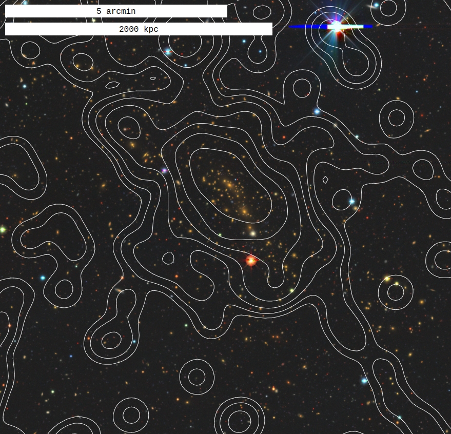
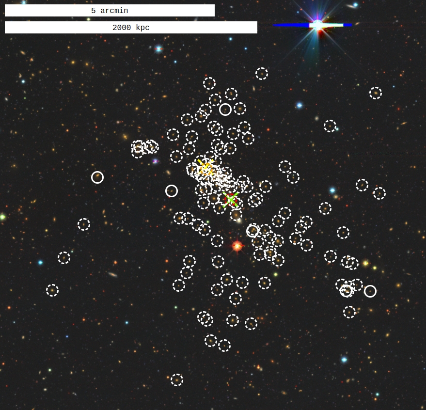
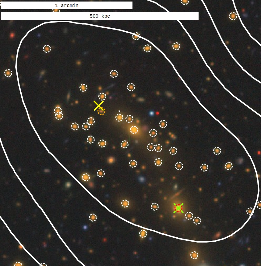
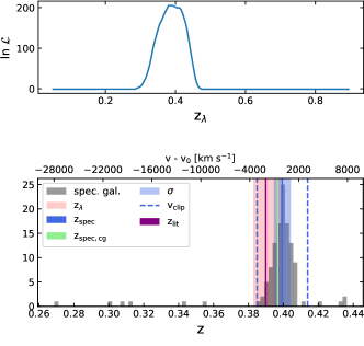
Figure 4: An illustrative example 1eRASS J041610.4-240351 from the eRASS1 cluster catalog. The panels in the top row show an LS $grz$ image of the full cluster overlaid with eRASS1 X-ray contours (left) and cluster members detected in this work (circles, right). Spectroscopic information is available for all cluster members marked by dashed circles. The bottom-left panel shows a zoom-in. The red circle marks the BCG, which agrees with the optical cluster center (green cross). The orange circle is located at the position of the central galaxy, which is the one closest to the X-ray center (yellow cross). North is up; east is left. In the bottom-right panel, upper subpanel, the cluster likelihood $\ln\mathcal{L}(z)$ shows one peak at $z=0.385$ which is close to the cluster photometric redshift $z_{\lambda}=0.3910\pm 0.0082$. The bottom-right panel, lower subpanel, demonstrates the measurements of the spectroscopic redshift and the velocity dispersion for the shown cluster. The cluster has a richness of $\lambda=128.7\pm 8.5$. The 127 photometric members are marked by circles. Of those, 121 have spectroscopic redshifts and are marked by dashed circles. The black histogram in the bottom panel shows the spectroscopic redshifts of the photometric members. Ten outlier galaxies with $z\gtrless z_{\rm spec}\pm 3\sigma$ (blue dashed lines) are discarded, leaving $N_{\rm members}=111$ spectroscopic members. The cluster velocity dispersion is $\sigma=1034\pm 67$ km s^-1 (light blue line). The photometric cluster redshift (light red shades) agrees with the spectroscopic cluster redshift $z_{\rm spec}=0.39936\pm 0.00039$ (darker blue line). The redshift of the galaxy at the optical center is $z_{\rm spec,cg}=0.3967\pm 0.0004$ (green line). The literature redshift $z_{\rm lit}=0.38989$ (purple line) is a photometric redshift from MARDY3 (Klein et al. 2019).

4 The eRASS1 Identified Cluster and Group Catalog

The main outcome of this work is the determination of the optical properties (redshifts, richnesses, etc.) of the galaxy clusters and groups detected in eRASS1. Most extended X-ray sources are genuine galaxy clusters. However, AGN (or other point sources), as well as random background fluctuations and supernova remnants, may be detected as extended sources, inducing contamination among the cluster candidates. The contamination rate is anti-correlated with the brightness of the source and its likelihood to be extended $\mathcal{L}_{\rm ext}$. Using simulations, Seppi et al. (2022) predicted that the purity is $\sim$97% ($\sim$50%) when considering a sample with $\mathcal{L}_{\rm ext}>3$ and above a flux limit of 8.0 (0.4) $\times 10^{-13}$ ergs s^-1 cm^-2. The eRASS1 cluster candidate catalog is not strictly flux-limited because of the spatially varying exposure time. However, an approximate flux limit is $F_{500}\approx 0.4\times 10^{-13}$ ergs s^-1 cm^-2 (Bulbul et al. A&A subm.). Depending on the science case, more or less pure and complete samples can be selected by applying cuts in $F_{500}$ or $\mathcal{L}_{\rm ext}$.

For the same flux thresholds, the completeness is expected to be $\sim$90% ($\sim$11.3%). Selecting cluster candidates with a higher threshold in $\mathcal{L}_{\rm ext}$ yields higher purity but at the cost of lower completeness for the same flux limit (see also Bulbul et al. A&A subm.). The threshold of $\mathcal{L}_{\rm ext}>3$ is applied in this work to prefer high completeness. The low purity for the low flux threshold is increased significantly in this work by requiring cluster candidates to be identified using optical and near-infrared imaging data.

In that process, we clean the eRASS1 cluster candidate catalog of 2,497 extended X-ray source detections for which we find no counterpart in the optical data, and of 458 detections which we classify visually as contamination. These results are achieved by running eROMaPPer in scan mode on the positions of all candidate galaxy clusters and groups in eRASS1.

We detail the procedure for constructing the catalog in Section 4.1 and describe its contents in Section 4.2.

4.1 Constructing the Catalog

In scan mode, we fix the cluster coordinates to the cataloged X-ray coordinates (R.A., Decl.). The member search radius is given in Equation (1). The eROMaPPer runs are done with different combinations of the $g$,$r$,$i$,$z$, and $w1$ filters. The optimal filter band combination changes with redshift. We find in Sections 8.1 and 8.2 that $grz$ performs well at low and intermediate redshifts $z_{\lambda}\leq 0.8$ while $grizw1$ is best suited for high redshifts $z_{\lambda}>0.8$. For the catalogs obtained in eROMaPPer scan mode, we merge the different runs afterward using a priority scheme.

The richness $\lambda$ measurement varies from run to run. That is because membership probabilities change when more filter bands are included and different galaxy luminosity cuts are applied. We calculate a normalized richness $\lambda_{\rm norm}$ where these systematic effects are corrected in Section 4.1.2.

4.1.1 Catalog Merging

Six different eROMaPPer runs are done on the eRASS1 cluster candidate catalog. Four of them for the southern LS in the filter band combinations $grz$, $griz$, $grizw1$, and $grzw1$, and two of them for the northern LS in the filter band combinations $grz$ and $grzw1$. No $i$-band data are available for the northern surveys. The resulting catalogs are merged using the following priority scheme:

$$1.\quad grz z_{\lambda}\leq 0.8 (10,\!823),$$ LS DR10 south if

$$2.\quad griz z_{\lambda}\leq 0.8 (314),$$ LS DR10 south if

$$3.\quad grz z_{\lambda}\leq 0.8 (202),$$ LS DR9   north if

$$4.\quad grizw1 z_{\lambda}>0.8 (485),$$ LS DR10 south if

$$5.\quad grzw1 z_{\lambda}>0.8 (113),$$ LS DR10 south if

$$6.\quad grzw1 z_{\lambda}>0.8 (7),$$ LS DR9   north if

$$7.\quad (303),$$ other

$$(12,\!247).$$

In parenthesis is the number of unique clusters for each category that went into the merged eRASS1 identified catalog. For example, in run 1, we find 10,823 unique clusters, while by adding the $i$ band (run 2), we find an additional 314 unique clusters. In the category “other” fall clusters that are either at $z>0.8$ and only detected in the $grz$ or $griz$ runs (114), or at $z\leq 0.8$ and only detected in the $grizw1$ or $grzw1$ runs (35). If they are detected in more than one run and are always outside the constrained redshift range (7), we still follow the priority scheme but neglect the redshift constraint. Moreover, we include clusters with no counterpart in the LS but are matched with a cluster from the literature (147).

The result is a robustly constructed catalog of the optical properties for 12,247 identified eRASS1 galaxy clusters and groups.

4.1.2 Richness Normalization

The cluster richness $\lambda$ is the sum of the membership probabilities $p_{{\rm mem},i}$ (see Equation (3)). It includes corrections for the masked area (see Appendix A.4) and the limited depth in the optical images. eROMaPPer was run for different filter band combinations with different luminosity thresholds. For the $grz$ and $griz$ runs, we select only galaxies with a minimum luminosity of $L>0.2$ L_∗, where L_∗ is the break of the Schechter luminosity function (Schechter 1976). This luminosity cut minimizes the scatter of the X-ray luminosity at fixed richness (Rykoff et al. 2012). For the $grzw1$ and $grizw1$ runs, we apply a higher minimum luminosity of $L>0.4$ L_∗ to have (a noisier but) unbiased richness at higher redshift $z>0.8$ (see Appendix B).

When the luminosity threshold increases, the richness is systematically smaller because fewer galaxies are selected. To correct for this effect, we define a normalized richness;

$$\lambda_{\rm norm}=S_{\rm norm}\lambda$$ (11)

and its uncertainty

$$\delta\lambda_{\rm norm}=S_{\rm norm}\delta\lambda.$$ (12)

It is determined by comparing the richness of the same clusters measured in different runs. The relations are fit by minimizing the uncertainty-weighted squared orthogonal distances to the best-fit line (Boggs et al. 1989). We also apply an orthogonal cut at low richness to not bias the slope. The resulting scaling factors are given in Table 2.

Filter Band Combination	$S_{\rm norm}$
$grz$ (DR10 south)	1.000
$griz$ (DR10 south)	1.039
$grz$ (DR9 north)	1.020
$grizw1$ (DR10 south)	2.451
$grzw1$ (DR10 south)	2.336
$grzw1$ (DR9 north)	2.550

Table 2: Richness scaling factors $S_{\rm norm}$ used to calculate the normalized richness $\lambda_{\rm norm}=S_{\rm norm}\lambda$. As the reference, we choose $S_{\rm norm}=1$ for the $grz$ filter bands in the LS DR10 south. The biggest impact on $S_{\rm norm}$ is the minimum galaxy luminosity of the cluster members. It is fainter for the $grz$ and $griz$ filter band combinations ($L>0.2$ L_⊙) than for the runs that include the $w1$ band ($L>0.4$ L_⊙). The richness increases when fainter members are included.

4.1.3 Assigning the BCG

Near the center of a galaxy cluster often resides a disproportionately bright and extended early-type galaxy called the Brightest Cluster Galaxy (BCG). These galaxies are distinct from normal massive early-type galaxies due to their embedding in the faint Intracluster Light (ICL, see recent reviews by Contini 2021; Arnaboldi & Gerhard 2022; Montes 2022).

The choice of the BCG can be ambiguous in $\sim$20% of the cases (Kluge et al. 2020). For simplicity, we define the BCG as the brightest member galaxy in the $z$ band. We explore the justification for this definition in Section 5.5.

4.2 Properties of the eRASS1 Catalog of Identified Clusters and Groups

In this section, we detail the overall statistics of the results obtained with the eROMaPPer runs on the eRASS1 cluster candidate catalog.

4.2.1 Cluster Identification Statistics

The eRASS1 source catalog covers half of the sky. It contains 26,682 extended sources (Merloni et al. 2024). After cleaning split sources and masking regions of known non-cluster extended X-ray sources (see Section 2.1 and Bulbul et al. A&A subm.), we obtain a sample of 22,718 cluster candidates with extent likelihood $\mathcal{L}_{\rm ext}>3$. We run eROMaPPer in scan mode on this sample and obtain optical properties (redshifts, richnesses, optical centers, and BCG positions) for 12,705 clusters.

Most of the rejected candidates (7,516) are outside of the LS footprint (see Figure 2 and Appendix A.4) and have no match to known clusters in the literature (see Section 3.4). A further 2,497 rejected candidates have LS coverage, but no optical red sequence counterpart has been found with eROMaPPer. These X-ray sources are most likely AGN or random background fluctuations misidentified as extended sources (Bulbul et al. 2022). We discuss the properties of these contaminating sources in Section 7. It is also possible that some real clusters are not optically identified because their redshift is higher than the limiting redshift of the LS $z\gg z_{\rm vlim}$. Finally, we perform a visual cleaning procedure as described in Section 4.2.2. This further reduces the sample to a final size of 12,247 eRASS1 clusters in a sky area of 13,116 deg², so an average density of about one cluster per square degree.

The association of the X-ray signal with the optical cluster is straightforward in 97% of the cases. For the remaining 332 eRASS1 clusters (3%) with $z_{\lambda}<z_{\rm vlim}$, we find overlapping structures in projection. A secondary photometric redshift $z_{\lambda,2}$ is provided in these cases. It is mentioned in Bulbul et al. (A&A subm.) that one eFEDS cluster (eFEDSJ091509.5+051521, Klein et al. 2022; Liu et al. 2022) has inconsistent redshift ($z=0.249$) to its counterpart 1eRASS J091510.9+051440 ($z_{\rm spec}=0.136$). We find that it agrees with $z_{\lambda,2}=0.269$.

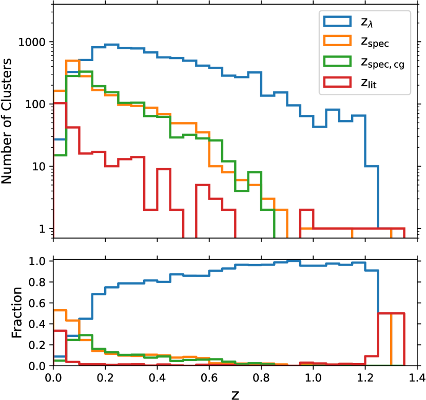
Figure 5: Number (top panel) and relative fraction (bottom panel) of eRASS1 clusters per redshift bin depending on their best redshift type. The total numbers are 8790 photometric redshifts ($z_{\lambda}$, Section 3.2), 1759 spectroscopic redshifts determined using the bootstrap method ($z_{\rm spec}$, Section 3.3), 1451 spectroscopic redshifts of the galaxy at the optical center ($z_{\rm spec,cg}$, Section 3.3), and 247 literature redshifts ($z_{\rm lit}$, Section 3.4). Clusters with unflagged velocity dispersion information (Section 3.6) have the same distribution as the $z_{\rm spec}$ sample.

Close but separate X-ray sources can have a large number of common members identified when their separation is smaller than the optical cluster radius $R_{\lambda}$. This leads to a small number of 413 (3%) eRASS1 clusters that share ¿70% of their members with another cluster that has a higher likelihood $\mathcal{L}_{\rm max}$. We mark the cluster with lower $\mathcal{L}_{\rm max}$ in the eRASS1 catalog by flagging it as SHARED_MEMBERS.

4.2.2 Cluster Redshifts

Each of the 12,247 eRASS1 clusters has at least one redshift assigned. In 5,428 cases where multiple redshifts are available, we follow a priority scheme to assign the best redshift $z_{\rm best}$ from up to four available redshift types (see Section 3.5). Table 3 summarizes the results for the eRASS1 identified catalog. Most values of $z_{\rm best}$ are photometric (72%). We perform a detailed analysis of the accuracy of the photometric redshifts in Section 8. Higher-quality spectroscopic redshifts are available for a significant fraction (26%). Literature redshifts are adopted only in rare cases (2%). Figure 5 shows the number of clusters per redshift bin with associated redshifts. At low redshifts $z<0.15$, more than half of the eRASS1 clusters have a reliable spectroscopic redshift. This number falls below 10% above $z>0.6$.

The spectroscopic redshifts are calculated using the robust bootstrapped bi-weight method (15%; see Section 3.3) or adopted from the spectroscopic redshift of the central galaxy (12%). We note that the formal uncertainties for the latter method underestimate the real cluster redshift uncertainties because individual cluster member galaxies can have a non-negligible line-of-sight velocity with respect to the cluster rest frame (see Section 3.3 and Figure 4). For the eRASS1 clusters, the mean offset velocity is 80% of the cluster velocity dispersion. This corresponds to a mean uncertainty of $\delta z=0.0013$.

Literature redshifts, when available, are adopted for clusters (a) outside of the LS footprint (126 cases), (b) within the LS footprint but without an optical detection (21 cases), (c) where we decided after visual inspection that the optical detection is in projection to the X-ray source (95 cases), or (d) at low or high redshifts where $z_{\lambda}$ is outside of the calibration range for the red sequence ($z<0.05$ and $z>1.2$, see Appendix C) and no spectroscopic redshift is available (5 cases). In total, 247 eRASS1 clusters have $z_{\rm best}=z_{\rm lit}$. The 21 matched clusters within the LS footprint but without optical detection by us, are (a) at very low redshift $z_{\rm lit}<0.05$ (14 cases), (b) at higher redshift than the limiting redshift of the LS (2 cases), (c) a very poor group (1eRASS J022946.2-293740), (d) consist only of late-type galaxies (1eRASS J091433.5+063417), or not detected for unknown reasons (1eRASS J050808.8-525124, 1eRASS J055136.2-532733, 1eRASS J102144.9+235552).

Pri.	Redshift Type	Notation	Total	Best
1	spectroscopic	$z_{\rm spec}$	1906	1759
	($\geq$3 members)
2	spectroscopic	$z_{\rm spec,cg}$	2881	1451
	(gal. at opt. center)
3	photometric	$z_{\lambda}$	12100	8790
4	literature	$z_{\rm lit}$	3886	247
Total				12,247

Table 3: Redshift types and occurrences in the eRASS1 catalog. The priorities in the first column and redshift types in the second and third columns are described in Section 3.5. The total number of available redshifts for each type is given in column four, and column five shows how often each redshift type is selected as the best redshift $z_{\rm best}$.

Furthermore, there are cases in which more than one cluster is projected near the X-ray emission. In these cases, eROMaPPer chooses the cluster with the highest likelihood $\ln\mathcal{L}_{\rm max}$, which correlates with the richness by definition. This is generally a good strategy when the galaxy sample is complete. However, we will show in Section 5.3 that the optical completeness drops below $z\lesssim 0.05$ because we discard galaxies near bright and extended galaxies. Consequently, if the cluster is at low redshift, eROMaPPer often chooses a background cluster. We identify these cases by

• matching all clusters with the NGC catalog (Dreyer 1888) using a 30″ search radius,

• looking for a secondary low-$z_{\lambda,2}$ peak in the $\ln\mathcal{L}(z)$ distributions (see Section 3.2),

• selecting clusters with low $z_{\rm lit}$,

• searching for close pairs in the X-ray images

and inspecting their X-ray images, optical images, and member galaxy distributions visually. For the cases that we judge to be misidentified, we set $z_{\rm best}=z_{\rm lit}$ if a literature redshift is available (87 cases). If no $z_{\rm lit}$ is available, we discard that cluster (371 cases).

4.2.3 eRASS1 Clusters in the Large-Scale Structure

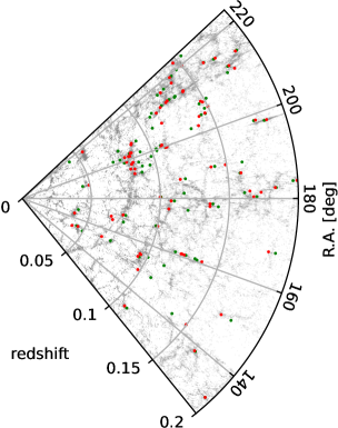
Figure 6: Slice of the cosmic volume with eRASS1 clusters with available spectroscopic redshifts $z_{\rm spec}$ overplotted onto our spectroscopic galaxy compilation (gray points). The slice has a thickness of $\pm 2\degr$ around ${\rm Decl.}=0\degr$. Red points mark the positions of eRASS1 clusters when spectroscopic redshifts are used. They trace the nodes of the cosmic web. Green points mark the same clusters, but this time, we use the photometric redshifts. They scatter around the nodes of the cosmic web because of the higher redshift uncertainty.

Massive galaxy clusters are located at the nodes of the cosmic web. Galaxies trace this web and can be visualized by selecting a thin slice limited in declination around $\pm 2\degr$. Figure 6 shows a zoom-in on the redshift range $0\leq z\leq 0.2$. We also restrict the range in right ascension ($125\degr<{\rm R.A.}<223\degr$) to the overlapping area in the western galactic hemisphere that is well covered by eROSITA (see Figure 2). Gray data points correspond to the redshifts of the galaxies in our spectroscopic compilation (see Sec. 2.3 and Appendix D). Three slices in R.A. have a high galaxy density. They correspond to the GAMA fields G09, G12, and G15 (Driver et al. 2022). Overplotted in green are the positions of the eRASS1 clusters when using their photometric redshifts. We will show in Section 8.2 that these redshifts have an uncertainty of $\delta_{z}\approx 0.005-0.015$. This is sufficiently large to cause an apparent displacement of the eRASS1 clusters from their true position in the cosmic web. The red points correspond to the same clusters but are located at their spectroscopic redshifts, with a $\sim$10 times higher precision (see Section 8). In these cases, the eRASS1 clusters trace the cosmic web well, as can be seen for example around $z\approx 0.08$ and ${\rm R.A.}\approx 200\degr$.

4.2.4 Consistency with Known Clusters

We match all eRASS1 cluster candidates with the public catalogs in Table 1 as described in Section 3.4 and find 3,886 pairs. The consistency of $z_{\rm best}$ with the matched $z_{\rm lit}$ is shown in Figure 7. We only consider clusters where the best redshift type is not the literature redshift and the masking fraction is below $<10\%$. The four colored lines refer to different allowed redshift deviations. Above a richness of $\lambda_{\rm norm}=20$, 94% of the matched clusters have consistent redshifts within $|z_{\rm best}-z_{\rm lit}|/(1+z_{\rm lit})<0.02$. The fraction increases to $>98\%$ with larger allowed redshift deviations $|z_{\rm best}-z_{\rm lit}|/(1+z_{\rm lit})<0.10$. The remaining inconsistencies are explained by ambiguous cluster choices in the presence of multiple structures along the line of sight (see Section 3.2.2). At low richness ($\lambda_{\rm norm}<20$), these ambiguous choices become more frequent because the purity decreases as we will show in Section 7. Here, about 80% (92%) of the matched clusters have consistent redshifts within $|z_{\rm best}-z_{\rm lit}|/(1+z_{\rm lit})<0.02$   ($<0.10$).

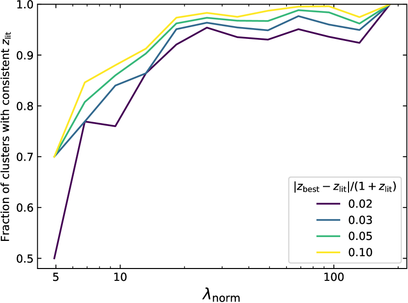
Figure 7: Fraction of eRASS1 clusters with consistent best redshift $z_{\rm best}$ and literature redshift $z_{\rm lit}$ depending on richness $\lambda_{\rm norm}$. Four different redshift tolerances are applied.

Surprisingly, two matched clusters with large richnesses $\lambda_{\rm norm}>100$ are inconsistent with the literature redshift. The first outlier, 1eRASS J094813.0+290709, is a rich cluster with $\lambda=133\pm 7$ at high redshift $z_{\lambda}=0.766\pm 0.013$. The eRASS1 X-ray signal is well centered on that cluster. Its matched counterpart in the CODEX catalog has a significantly lower redshift $z_{\rm lit}=0.253$ and lower richness $\lambda_{\rm lit}=19\pm 2$. We identify another cluster in close proximity (2.4′ east) in our blind-mode eROMaPPer catalog, which we describe in Section 6.1. Its redshift $z_{\rm spec}=0.254$ is consistent with the CODEX redshift. One likely reason for the different choices is the limited depth. CODEX is limited to a lower redshift range $z\lesssim 0.6$ because it relies on shallower SDSS data where the high-$z$ cluster is not visible. Another possibility is miscentering. CODEX relies on ROSAT data with a much larger PSF. This could have played a role in determining the cluster center in the CODEX catalog.

The second outlier, 1eRASS J020628.4-145358 (Abell 305), has a robust redshift of $z_{\lambda}=0.298\pm 0.006$. Its matched counterpart MCXC J0206.4-1453 is at $z_{\rm lit}=0.153$. The literature redshift was measured using spectroscopic redshifts of two galaxies (Romer 1994). We identify one late-type galaxy LEDA 918533 close ($\approx 20\arcsec$) to the eRASS1 X-ray emission peak, which could be a foreground galaxy that has been misclassified as a cluster member by Romer (1994).

4.2.5 Cluster Velocity Dispersions

For all eRASS1 clusters with at least three spectroscopic member galaxies, we calculate the cluster velocity dispersion $\sigma$ as the line-of-sight velocity dispersion of those galaxies. The total number of eRASS1 clusters with an estimated velocity dispersion is identical to the number of 1906 clusters with available spectroscopic redshift $z_{\rm spec}$ (see Table 3). However, the flagging is stricter. For $z_{\rm spec}$, we require the velocity clipping of the full sample of spectroscopic members to converge. For $\sigma$, we require the velocity clipping for all bootstrapped realizations to converge. This gives more robust results by reducing the number of clusters with substructure. Of the 1,906 spectroscopic clusters, 1,499 are not flagged and, hence, have robust $\sigma$ estimates.

The clusters with robust $\sigma$ estimates against redshift are similar to the distribution shown for $z_{\rm spec}$ in Figure 5 by the orange line. We do not show the histogram for $\sigma$ explicitly.

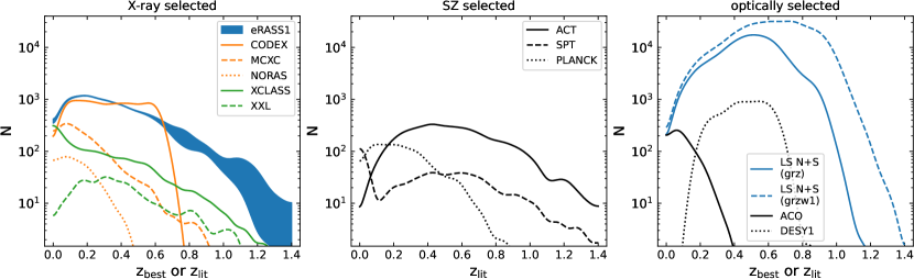
Figure 8: Number of clusters per redshift interval $\Delta z_{\lambda}=0.05$. For catalogs created in this work (blue), we use the best redshift $z_{\rm best}$, and for literature catalogs, we use the published redshift $z_{\rm lit}$. Each panel refers to a different cluster selection method. The smoothed histograms are obtained by summing over the redshift posteriors of all clusters. For better visibility, the distributions are additionally smoothed with a Gaussian kernel with a standard deviation $\Delta z_{\lambda}=0.04$. For the eRASS1 catalog, the upper border of the filled region refers to all 12,247 clusters, and the lower border refers to the subset of 10,959 clusters with $z_{\lambda}<z_{\rm vlim}$. A richness cut $\lambda_{\rm norm}>16$ and a limiting redshift cut $z_{\lambda}<z_{\rm vlim}$ are only applied to the optically selected combined LS DR10 south and LS DR9 north catalogs (LS N+S). That makes them comparable to the DES year 1 catalog, which has a consistent richness cut of $\lambda>20$ applied (see Section 5.4).

Of those 1,499 clusters, 358 have a high-quality velocity dispersion value calculated with the bi-weight scale estimator (see Section 3.6). As we require a large number of $N_{\rm members}\geq 15$ spectroscopic members for this method, these values have a low relative uncertainty: $\delta\sigma/\sigma\sim 20\%$. The remaining 1,141 velocity dispersions were calculated with the gapper estimator. The relative uncertainties are on the order of $\delta\sigma/\sigma\sim 40\%$.

In total, 6.5% of the photometric members with spectroscopic redshift information are discarded by the velocity clipping procedure.

5 Quality Assessments of the eRASS1 Catalog

In addition to the eRASS1 catalog, we run eROMaPPer in scan mode on various catalogs of candidate clusters from the literature, selected using different methodologies. By doing so, we can compare our results to the redshifts and richnesses measured in previous works. In addition to this, we ran eROMaPPer in blind mode on the full LS DR10 south and LS DR9 north. This enables the analysis of selection effects that arise purely from the processing of the optical and near-infrared data. These effects can manifest as a depth-dependent contamination rate and possible deviations of the cluster number density from a theoretical halo-mass function.

The input catalogs used are listed in Table 4. These include clusters that are selected using their X-ray signal: CODEX (Finoguenov et al. 2020), MCXC (Piffaretti et al. 2011), NORAS (Böhringer et al. 2017), XXL (Adami et al. 2018), XCLASS (Koulouridis et al. 2021), using the Sunyaev Zeldovich (SZ) effect: ACT (Hilton et al. 2020), SPT (Bleem et al. 2015), Planck (Planck Collaboration et al. 2016b), or via optical overdensities of galaxies: ACO (Abell et al. 1989), DES (Abbott et al. 2020). The number of clusters contained in these catalogs against redshift is shown in Figure 8. Approximate footprints are shown in Figure 9. Black heal pixels, each covering an area of 13.4 deg², are within the footprint of the LS, and gray heal pixels are outside of them. Patchy maps indicate a low number density of clusters.

Survey	Source	Cataloged	In LS	Survey Area
		Clusters	Footprint	[deg2]
X-ray selected
eRASS1	Bulbul et al. (A&A subm.) & this work	12,247	12,247	13,116
CODEX	Finoguenov et al. (2020)	10,382	10,079	10,269
MCXC	Piffaretti et al. (2011)	1743	1477	$\sim$all sky
NORAS	Böhringer et al. (2017)	378	344	13,519
XXL	Adami et al. (2018)	302	299	50
XCLASS	Koulouridis et al. (2021)	1559	1433	269
SZ selected
ACT	Hilton et al. (2020)	4195	4044	13,211
SPT	Bleem et al. (2015)	677	656	2500
PLANCK	Planck Collaboration et al. (2016b)	1653	1207	$\sim$all sky
optically selected
LS DR10 south $grz$	this work	112,609	112,609	19,342
LS DR10 south $grzw1$	this work	273,150	273,150	19,342
LS DR10 south $griz$	this work	91,790	91,790	15,326
LS DR10 south $grizw1$	this work	242,044	242,044	15,326
LS DR9 north $grz$	this work	27,516	27,516	5068
LS DR9 north $grzw1$	this work	93,227	93,227	5068
ACO	Abell et al. (1989)	5250	4635	$\sim$all sky
DESY1	Abbott et al. (2020)	6729	6724	1437

Table 4: Overview of the catalogs analyzed with eROMaPPer in this work. The survey area is calculated from the high-resolution HEALPix maps for eRASS1 and the optically selected LS catalogs or taken from the catalog paper in the source column. Three catalogs have survey areas that cover approximately the full sky but (partly) exclude the galactic plane, as shown in Figure 9. A richness cut of $\lambda_{\rm norm}>16$ and a redshift constraint $z_{\lambda}<z_{\rm vlim}$ are applied to the LS DR9 north and LS DR10 south catalogs. Although the number of detections is huge, the contamination fraction in these catalogs is not well known.

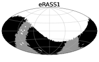
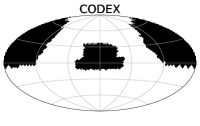
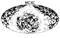
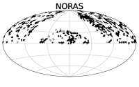
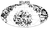
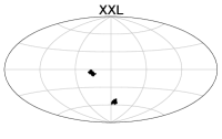
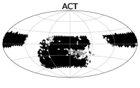
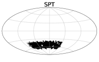
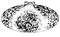
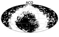
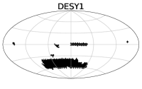
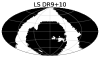
Figure 9: Footprint maps for the cluster catalogs used in this work. The HEALPix resolution is ${\rm NSIDE}=16\leavevmode\nobreak\ \hat{=}\leavevmode\nobreak\ 13.4$ deg². Black regions overlap with the LS footprint and gray regions are outside of it. White holes within the footprint indicate that the local cluster number density in a catalog is less than 1 per heal pixel.

5.1 Comparison to other X-ray-Selected Catalogs

We show the number of eRASS1 clusters against redshift $z_{\rm best}$ as the blue line in Figure 8, left panel. The median redshift of the eRASS1 sample is $z_{\rm best}=0.31$, and the highest is $z_{\rm best}=1.32$ (1eRASS J020547.4-582902). The line width increases toward higher redshift. Its upper border corresponds to the full sample of 12,247 clusters. The lower border corresponds to the subsample of 10,959 clusters with $z_{\lambda}<z_{\rm vlim}$; that is, the photometric redshift must be below the local limiting redshift of the LS (see Appendix B). We explore the increasing contamination associated with exceeding the limiting redshift in Section 6.6.

The eRASS1 cluster catalog contains the largest number of identified clusters of all considered literature catalogs (see Table 4). Compared to other X-ray-selected catalogs, the advantage is the larger survey area than XMM-Newton (green lines in Figure 8, see also Figure 9 and Table 4) and the better sensitivity and smaller PSF than ROSAT (orange lines in Figure 8).

For CODEX, the source detection on RASS data was improved, reaching a similar depth to eRASS1. The contamination in the cluster candidate sample is high but the published catalog was already cleaned by identifying the candidates using redMaPPer and SDSS data. A great advantage of eROSITA over ROSAT is that the sharper PSF is better suited to filter sources at high redshift by their extent, leading to purer cluster samples. Moreover, the CODEX sample is limited in redshift to $z\lesssim 0.6$ by the usage of shallower SDSS imaging data.

5.2 High-$z$ Optical Completeness

We estimate the high-$z$ completeness of the eRASS1 identified catalog using SZ-selected catalogs. The SZ signal is independent of redshift, which is exploited to produce highly complete catalogs with 90% completeness for $M_{500\rm{c}}>3.8\times 10^{14}$ M_⊙ at (ACT, Hilton et al. 2020) or nearly 100% completeness for $M_{500\rm{c}}>7\times 10^{14}h_{70}^{-1}$ M_⊙ at $z>0.25$ (SPT, Bleem et al. 2015). Figure 8, middle panel, confirms that the number of clusters remains large at high literature redshift in the ACT, SPT, and Planck catalogs. Hence, they are well suited for testing the optical completeness of high-$z$ clusters in the eRASS1 catalog. For this, we run eROMaPPer in scan mode on the locations of the literature clusters. We define the optical completeness $C$ as the number of eROMaPPer-identified clusters $N_{\rm lit\&ero}$ to the total number of clusters $N_{\rm lit}$ in the SZ-selected literature catalogs

$$C(z)=\frac{N_{\rm lit\&ero}(z)}{N_{\rm lit}(z)}.$$ (13)

Thereby, we only consider clusters that lie within the LS footprint. Furthermore, the literature redshift must be lower than the limiting redshift of the LS $z_{\rm lit}<z_{\rm vlim}$. To avoid mismatches in the cases of overlapping clusters, we require $|z_{\rm best}-z_{\rm lit}|<0.1$ for a cluster to be considered a match. Figure 10, right panel, confirms a high optical completeness $C>0.95$ for $z_{\lambda}<1.1$. We emphasize that the optical completeness does not take the completeness of the X-ray source catalog into account (see Section 4). It is solely sensitive to the processing of the optical and near-infrared data.

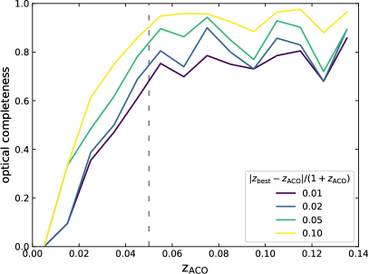
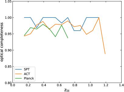
Figure 10: Optical completeness defined as the ratio of clusters confirmed after running eROMaPPer in scan mode on the cluster coordinates in various catalogs from the literature. At low redshifts, we use the ACO catalog and quantify the completeness for four different redshift tolerances. At high redshifts, we use the SPT, ACT, and Planck catalogs and consider clusters as confirmed when the redshifts agree within $|z_{\rm best}-z_{\rm lit}|/(1+z_{\rm lit})<0.1$. We restrict the samples to clusters where the LS are sufficiently deep, that is, $z_{\rm best}<z_{\rm vlim}$. A minimum of five clusters is required per redshift bin.

The median richness is $\lambda_{\rm norm}=50$ for the ACT and SPT catalogs. For Planck, it is $\lambda_{\rm norm}=70$, which explains the lower number of clusters even though it is an all-sky survey. In the eRASS1 catalog, the median richness is lower with $\lambda_{\rm norm}=25$ because eROSITA is more sensitive to galaxy groups, especially at low redshift (Bahar et al. 2024).

5.3 Low-$z$ Optical Completeness

We estimate the low-$z$ completeness of the eRASS1 identified catalog with the help of the optically selected ACO catalog (Abell et al. 1989). This was compiled by visually inspecting photographic plates and is more sensitive to lower redshift. For the following investigation, we select 577 ACO clusters with a cataloged redshift $z_{\rm ACO}<0.14$ and lie in the LS footprint. Additionally, we include 16 ACO clusters that are formally outside of the footprint. However, they are only classified as such because the clean region around the BCG was masked due to the assigned MASKBITS (see Sections 2.2.3 and 3.1).

Figure 10, left panel, shows the ratio of ACO clusters confirmed after running eROMaPPer in scan mode on the ACO coordinates over total ACO clusters. The redshift $z_{\rm ACO}$ is taken from the ACO catalog. The yellow curve demonstrates a high optical completeness of $C\approx 95\%$ beyond $z_{\rm ACO}>0.05$. Below $z_{\rm ACO}<0.05$, the optical completeness drops steeply: of 185 ACO clusters, we confirm 132 ($C=71\%$). The optical limitation stems from the LS photometry around bright extended galaxies. While we keep galaxies in the Siena Galaxy Atlas, we exclude those that overlap. These optical detections are often spurious. The consequence of the removal is that a background cluster is often preferred over a low-$z$ cluster.

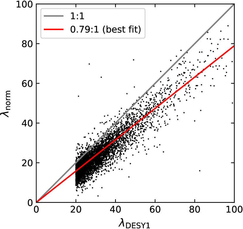
Figure 11: Comparison between the richnesses $\lambda$ measured using eROMaPPer and the published richnesses for the same DES year 1 clusters. The 1:1 relation is shown in gray and the red line is the best-fit linear relation with a slope of $\alpha=0.79$.

5.4 Richness Comparison

The DES year 1 catalog was created using the cluster finder redMaPPer, similar to this work (Abbott et al. 2020). This allows a direct comparison of the measured richnesses. The catalog was obtained in redMaPPer blind mode, that is, without positional priors. The redshift range is limited to $0.2<z_{\lambda}<0.65$. Figure 11 compares the richnesses computed in this work $\lambda_{\rm norm}$ against the published richnesses $\lambda_{\rm DESY1}$ (Abbott et al. 2020). We use 4,716 clusters with good redshift agreement $\Delta z/(1+z_{\lambda})<0.01$, a low masking fraction (¡10%), and which are identified in the LS DR10 south using the $grz$ filter band combination, for which $\lambda=\lambda_{\rm norm}$ (see Section 4.1.2 and Table 2).

To compute the systematic scaling factor, we fit a linear relation to the data points by minimizing the orthogonal residuals. To avoid biases due to the sharp richness cut at $\lambda_{\rm DESY1}=20$, we make an additional orthogonal cut below the line defined by $\lambda_{\rm norm}<-1/\alpha\cdot\lambda_{\rm DESY1}+50$, where $\alpha=0.79$ is the best-fit slope. This procedure rejects 365 additional data points. We obtain the best-fit relation;

$$\lambda_{\rm norm}=0.79\cdot\lambda_{\rm DESY1}.$$ (14)

The richnesses measured in this work are, on average, 21% lower for identical DES year 1 clusters. A possible explanation is the different handling of galaxy outliers with respect to the red-sequence model in earlier versions of redMaPPer. We do not correct for this effect.

5.5 BCG Selection

Three common defining qualities of a BCG (being the brightest, most extended, and most central member) can conflict in up to 20% of the cases, especially when shallow photometry is used (Von Der Linden et al. 2007; Kluge et al. 2020). Moreover, merging or unrelaxed clusters can have significantly miscentered BCGs. We explore three options for selecting the BCG:

1. located at the X-ray center,

2. located at the optical cluster center,

3. being the brightest member.

Figure 4 shows an illustrative example. The zoomed image in the bottom-left panel is centered on the galaxy, which visually fulfills best the common BCG selection criteria. It is also well-centered in the X-ray contours (white). The location of the initial X-ray detection in the catalog (before refined modeling, Bulbul et al. A&A subm.) is shown by the yellow cross. The nearest galaxy is marked by an orange circle. It is clearly not a good choice for the BCG. The BCG chosen by eROMaPPer (the brightest member galaxy) is marked by the red circle. It coincides with the optical center (green cross) but is inconsistent with our visual preference.

However, visual inspection of other clusters, especially from intermediate redshift upward, showed that selecting the brightest member as the BCG is a good choice in almost all cases. Consequently, we define the BCG in this work as the brightest member galaxy within $R_{\lambda}$ (see Equation (1)).

To evaluate the automatic BCG choice at low redshift $z<0.1$, we run eROMaPPer on the cluster catalog of Kluge et al. (2020). This catalog is mostly a subset of the ACO catalog, but each cluster is carefully centered on the BCG. The BCG was chosen as the largest and most central galaxy based on visual inspection of deep images that reveal visual features on levels 27–28 $g^{\prime}$ mag arcsec^-2. Of the 154 cataloged clusters that are within the LS footprint, we identify 130 cases with consistent redshift ($|z_{\rm best}-z_{\rm lit}|<0.01$). The lost fraction is attributed to the growing incompleteness at low redshifts (see Section 5.3). The median redshift of the sample from Kluge et al. (2020) is $z=0.06$. Of the 130 clusters, our automatic BCG selection is in 85 cases, consistent with the choice made by Kluge et al. In 23 cases, the BCG is not a member galaxy according to eROMaPPer, even though its redshift is consistent with the cluster redshift. These BCGs are typically marginal outliers in color space. By only considering the remaining 107 clusters, the agreement with the BCG choice by Kluge et al. is 80%, precisely what we expect (see above). Higher color uncertainties at intermediate or higher redshift will likely keep the BCG colors consistent with the red-sequence colors. Therefore, we expect for the full eRASS1 and reanalyzed literature samples that the selected BCG is a good choice in $\sim$80% of the clusters.

6 Number Densities & Mass Limits

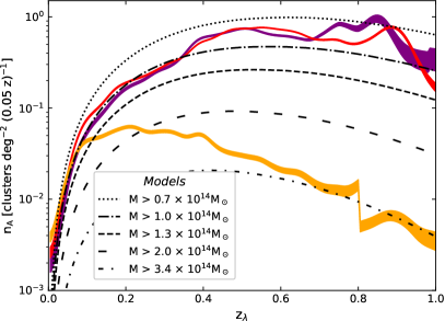
Figure 12: Cluster number density per sky area (left) and comoving volume (right) against redshift. Red and purple lines refer to clusters detected using the eROMaPPer blind mode on the LS DR10 south and LS DR9 north, respectively, in the $grz$ filter band combination. We restrict the samples to a reliable redshift range $z_{\lambda}<z_{\rm vlim}$. The orange line refers to the eRASS1 clusters. A discontinuity at $z_{\lambda}=0.8$ arises from the merging of the low-$z$-optimized and high-$z$-optimized eROMaPPer runs (see Section 4.1.1). A richness cut of $\lambda_{\rm norm}>16$ was applied only to the LS DR9 north and LS DR10 south catalogs. Volume densities for the SDSS DR8 and DES SVA catalogs are adopted from Rykoff et al. (2016) and for DES year 1, calculated assuming a survey area of 1437 deg² with uniform depth (see Table 4). The curves are normalized for a bin size of $\Delta z=0.05$ and smoothed using a Gaussian kernel with a standard deviation of $\Delta z=0.02$. The width of the lines corresponds to the Poissonian error for the same bin size, consistently as in Rykoff et al. (2016).

The eRASS1 cluster catalog’s lower mass limit increases with redshift due to a combination of the lower total flux received and the effect of cosmic dimming of the X-ray surface brightness in more distant clusters. Only the most luminous clusters can be detected at high redshifts. This behavior is quantified in our X-ray selection function (Clerc et al. A&A subm.).

An additional inhomogeneous optical selection function can alter the cluster catalog further. We examine its effect using the catalogs created with eROMaPPer in blind mode. This mode does not use positional priors. Hence, the obtained catalogs allow us to investigate purely optical selection effects. Our analysis utilizes the full LS DR9 north and LS DR10 south surveys, making the blind-mode cluster catalog the most extensive to date (see Figure 8 and Table 4). The crucial disadvantage is, however, that the selection function is not well known. This knowledge is imperative to perform precise cosmological studies, for which eROSITA was designed.

Number densities are computed by dividing the number of clusters per redshift bin by the survey area or comoving volume. The usable survey area depends on redshift because of the non-uniform depth of the LS. Therefore, we use the dashed curves in Figure 3 to calculate the redshift-dependent survey area and comoving volume for the eROMaPPer blind-mode catalogs.

6.1 Construction of Blind-Mode Catalogs

As described in Section 4.1.1, we run eROMaPPer in blind mode on six independent filter band and survey combinations. We do not merge the resulting catalogs because the clusters are not detected at the exact same locations in the different runs. Table 4 lists the total number of detected clusters for each run. We restrict the blind-mode samples to a reliable redshift range $z_{\lambda}<z_{\rm vlim}$. Moreover, we remove galaxy groups to increase the purity. Therefore, we are restricting the richness to $\lambda_{\rm norm}>16$, which corresponds to a halo mass restriction of $M_{\rm 200m}\gtrsim 10^{14}$ M_⊙ (see Section 4.1.2 and McClintock et al. 2018).

The resulting blind-mode catalog for the $grz$ filter bands contains 140,125 sources, 112,609 + 27,516 from the LS DR10 south and LS DR9 north, respectively. Another blind-mode catalog optimized for high redshifts using the $grzw1$ filter bands contains 366,377 sources (273,150 + 93,227). More details are given in Table 4.

6.2 Resulting Catalogs

The number of blind-mode clusters against redshift is shown by the blue lines in Figure 8, right panel. The continuous (dashed) line corresponds to the $grz$ ($grzw1$) catalog for the combined LS DR9 and LS DR10 survey areas. For the $grzw1$ runs, we only consider brighter galaxies $L>0.4$ L_∗ (compared to $L>0.2$ L_∗ for the $grz$ runs), which increases the usable survey volume (see Appendix B). Below $z_{\rm best}<0.4$, the $grz$ and $grzw1$ runs have the same effective survey area (see Figure 3). If there was no contamination and perfect completeness, the continuous and dashed lines should agree. The fact that they disagree indicates a higher level of contamination in the $grzw1$ run compared to the $grz$ run. This is expected because the higher galaxy luminosity threshold allows for less secure detections. At high redshift ($z_{\rm best}>0.6$), the lines begin to deviate much more from each other. The reason is the larger effective survey area for the $grzw1$ runs (see Figure 3). Number densities per area ($n_{\rm A}$, left panel) and volume ($n_{\rm V}$, right panel) are shown in Figure 12. The red (purple) curve corresponds to the LS DR10 south (DR9 north) $grz$ catalog. We find that the number density profiles for the clusters detected in the LS DR9 north and LS DR10 south are consistent within the amplitude of the systematic oscillations. The oscillations are larger than the statistical uncertainties and arise from the redshift-dependent redshift bias. We perform a detailed analysis in Section 8.1.

6.3 Comparison to Literature

Table 4 lists the total number of clusters for various catalogs used in this work. The sample size of the eROMaPPer blind-mode catalogs surpasses the DES year 1 sample size by a factor of 10 in the overlapping redshift range $0.2<z_{\rm best}<0.65$ (see Figure 8). The main reason for this improvement is the $\sim$10 times larger survey area of the LS compared to the DES year 1 area as listed in Table 4 and shown in the last two panels in Figure 9.

We compare our obtained volume number densities with results for the DES SVA (dark gray, $z_{\lambda}>0.2$) and SDSS DR8 (light gray, $0.08<z_{\lambda}<0.33$) by adopting the volume number densities from Rykoff et al. (2016). Additionally, we calculate the number densities for the public DES year 1 cluster catalog (black, $0.2<z_{\lambda}<0.65$) assuming a redshift-independent survey area of 1,437 deg² (see Table 4). All curves are consistent with each other within the amplitude of the systematic oscillations.

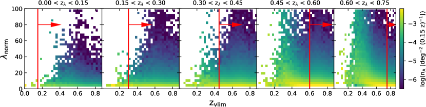
Figure 13: Dependency of the cluster number density on survey depth. The cluster number density per sky area $n_{\rm A}$ is calculated for the clusters detected using the eROMaPPer blind mode in the LS DR10 south using the $grz$ filter bands. The data is split into five bins in photometric cluster redshift $z_{\lambda}$. For each redshift bin, the densities are calculated for bins in limiting redshift $z_{\rm vlim}$ and richness $\lambda_{\rm norm}$. We consider the cluster properties reliable when local survey depth is sufficiently deep, that is, $z_{\lambda}<z_{\rm vlim}$ (see Appendix B for details). Those clusters are located to the right of the red line where the number density does not depend on $z_{\rm vlim}$. The number density left of the red line increases, which indicates a growing number of false-positive detections.

6.4 Comparison to Theoretical Halo Masses

For the LS cluster catalogs obtained in eROMaPPer blind mode, we apply a richness cut. As richness correlates with halo mass, we compare the number densities with halo model predictions. We compute theoretical number densities by integrating the halo mass function (Tinker et al. 2008; Diemer 2018) above five different mass limits.

The results are overlaid on Figure 12 with black lines. The mass limit $M\gtrsim 10^{14}$ M_⊙ (densely dash-dotted line) corresponds to our richness cut of $\lambda_{\rm norm}>16$ that is applied to the blind-mode catalogs (red and purple lines). The curves agree with the amplitude of the systematic oscillations. We conclude from the comparison that the impact of the optical selection function is small above $M\gtrsim 10^{14}$ M_⊙ because the observed number densities are consistent with the prediction.

We note that the predicted and observed number densities depend on cosmology. Applying the eRASS1 cosmology ($H_{0}=67.77$ km s^-1 Mpc^-1, $\Omega_{\rm m}=0.29$, and $\sigma_{8}=0.88$, Ghiradini et al. A&A subm.) shifts the predicted curves slightly upward.

6.5 Conclusions for eRASS1

We overplot the number densities for the eRASS1 clusters in Figure 12 in orange. They agree with the blind-mode sample below $z_{\lambda}\lesssim 0.1$ and the predictions for a mass limit $M\lesssim 10^{14}$ M_⊙ at $z_{\lambda}<0.1$. Beyond that, the number densities of the eRASS1 sample are lower, as expected. The sensitivity of eROSITA decreases for groups at higher redshift because of their low X-ray flux. The eRASS1 mass limit corresponds to $M\gtrsim 2\times 10^{14}$ M_⊙ at $z_{\lambda}=0.2$ and $M\gtrsim 3\times 10^{14}$ M_⊙ at $z_{\lambda}=0.8$.

The intercepts between the eRASS1 number densities and the model predictions roughly agree with the redshift-dependent mass limits of the eRASS1 sample, obtained from the scaling relation between X-ray count rate and weak lensing shear (Ghiradini et al. A&A subm.). The detection likelihood decreases toward higher redshifts and lower masses. This behavior is accounted for in the X-ray-selection function (Clerc et al. A&A subm.).

At $z_{\lambda}=0.8$, we notice a discontinuity in the eRASS1 cluster number surface density. It arises from the merging of the catalogs obtained for different filter band combinations (see Section 4.1.1).

6.6 Dependency on LS Survey Depth – Richness Bias

We utilize the blind-mode catalog obtained in the LS DR10 south ($grz$) further to demonstrate that the survey depth has no significant effect on the cluster number densities as long as only clusters with $z_{\lambda}<z_{\rm vlim}$ are selected, where $z_{\rm vlim}$ is the spatially dependent limiting redshift of the LS. Figure 13 shows the blind-mode cluster numbers per sky area binned in intervals of limiting redshift $z_{\rm vlim}$ and richness $\lambda_{\rm norm}$ for five cluster redshift bins. The measured cluster number density increases where the LS is too shallow for the considered redshift (see Appendix B). This effect must arise from measurement errors because the intrinsic cluster number density should not directly depend on the survey properties. A plausible explanation is an increasing number of false-positive member galaxies in shallower survey areas. This can occur due to the negative low-mass slope of the galaxy luminosity function (e.g., Blanton et al. 2005), which can lead to an increasing Eddington bias. Moreover, higher uncertainties in color can lead to an increased misidentification of interloping galaxies, or even stars, as cluster members. This can statistically inflate cluster richnesses, consequently increasing the observed cluster number densities. The affected clusters can be avoided by selecting only systems with photometric redshift lower than the local limiting redshift $z_{\lambda}<z_{\rm vlim}$. The red line in Figure 13 marks the required minimum depth for each cluster redshift bin. The red arrow indicates the direction to where the reliable clusters are located.

7 Purity of the eRASS1 Cluster Catalog

The eRASS1 catalog was optimized for high completeness by selecting cluster candidates above a low extent likelihood threshold $\mathcal{L}_{\rm ext}>3$. The trade-off is high contamination. Using this selection, we expect from simulations (Seppi et al. 2022) that only $\sim$50% of the extended sources are genuine galaxy clusters above the approximate eRASS1 flux limit of $F_{500}\approx 4\times 10^{-14}$ ergs s^-1 cm^-2 (Bulbul et al. A&A subm.). Most other sources are misclassified point sources, such as AGNs (and stars). A smaller contribution comes from random background fluctuations (Seppi et al. 2022).

In the optical, these contaminants can either have a non-detection of a red sequence with eROMaPPer (2,497 eRASS1 extended sources in the LS footprint, see Section 4.2.1), or be associated with an overdensity of red galaxies. In the latter case, these are either (a) line-of-sight projections of galaxies that are not bound to one cluster or (b) real overdensities of red galaxies around AGN as galaxies tend to cluster. We consider these sources as contaminants because the X-ray signal is not associated with the ICM.

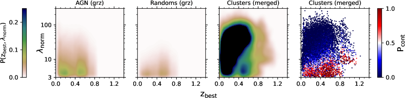
Figure 14: Kernel density estimates of AGNs, random points, and clusters in redshift ($z_{\rm best}$)–richness ($\lambda_{\rm norm}$) space (first three panels). The right panel shows the individual cluster data points color-coded by their probability of being a contaminant.

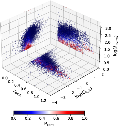
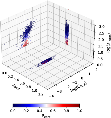
Figure 15: Distribution of clusters in redshift ($z_{\rm best}$)–richness ($\lambda_{\rm norm}$)–X-ray count rate ($C_{\rm R,X}$) space. The left panel shows the full distribution, and the right panel shows a slice in redshift $0.4<z_{\rm best}<0.5$ to enhance the dependence on the $\lambda_{\rm norm}$–$C_{\rm R,X}$ relation. The data points are projected on each side of the canvas. The probability of being a contaminant $P_{\rm cont}$ is color-coded. The top-right projection is equivalent to Figure 14, right panel.

To quantify the remaining contamination in the eRASS1 cluster catalog after our optical identification procedure, we introduce a mixture model in Ghiradini et al. (A&A subm.) (see also Bulbul et al. A&A subm.). It compares the properties of contaminants to those of clusters and attributes a probability $0\leq P_{\rm cont}\leq 1$, quantifying how likely each individual cluster is to be a contaminant. A detailed mathematical description of this mixture model can be found in Ghiradini et al. (A&A subm.). In this work, we provide details on the optical properties of the contaminating sources and how they are used to estimate the contamination probability of the eRASS1 clusters.

To estimate the contribution of both types of contaminants, we run eROMaPPer on 1,250,795 eRASS1 point sources (Merloni et al. 2024) and 1,000,000 random positions in the sky. Overdensities of red-sequence galaxies are identified for $\sim$850,000 and $\sim$490,000 sources, respectively. The exact numbers depend on the filter band combination. Random points are positioned at least five cluster radii $R_{\lambda}$ away from extended eRASS1 sources. We analyze the distribution of the randoms and eRASS1 point sources in redshift and richness space (see Figure 14, first two panels). The majority of the contaminants lie at low richnesses, as expected. We identify two peaks around $z_{\rm best}\approx 0.2$ and $z_{\rm best}\approx 0.5$. They are similarly pronounced for the point sources, while for the randoms, the second peak is slightly more dominant. The second peak is also apparent in the cluster sample (third panel). It indicates that there is indeed contamination left in the eRASS1 cluster catalog after the optical cleaning was performed in this work.

The global amplitudes of the kernel density estimates for both types of contaminants are fitted in the mixture model (Ghiradini et al. A&A subm.). For the primary eRASS1 cluster sample with $\mathcal{L}_{\rm ext}>3$, we obtain a three times higher amplitude for the point sources $f_{\rm AGN}=0.0768$ than for the randoms $f_{\rm rand}=0.0246$. This aligns with the expectation that most of the contamination in the eRASS1 cluster candidate catalog arises from X-ray point sources (Seppi et al. 2022).

Even though the distributions for the point sources and random points are similar in $z_{\rm best}$–$\lambda_{\rm norm}$ space, we can disentangle their contributions using the X-ray count rate $C_{\rm R,X}$. Figure 15 shows three projections of the 3-D distribution of the eRASS1 clusters in $z_{\rm best}$–$\lambda_{\rm norm}$–$C_{\rm R,X}$ space. The contamination probability $P_{\rm cont}$ is color-coded. AGNs typically have a higher X-ray flux than random background fluctuations. We model the $\lambda_{\rm norm}$–$C_{\rm R,X}$ distribution empirically using a redshift-dependent Schechter function (Schechter 1976). Thereby, we assume the power-law component to be the relation for clusters because both properties depend on the halo mass. Given this assumption, the exponential drop-off is due to the contamination. These objects are prominent in the right panel of Figure 15 as red points at low richnesses and high X-ray flux. It shows a selected redshift slice between $0.4<z_{\rm best}<0.5$. By averaging the $P_{\rm cont}$ values of all $N=12,247$ eRASS1 clusters, we calculate the residual contamination of the eRASS1 catalog to be

$$\sum_{i}{P_{\rm cont,i}}/N=14\%.$$ (15)

Using this result, we also compute the purity of the eRASS1 cluster candidate catalog (before optical identification). There are 16,336 cluster candidates in the LS footprint and $N\cdot\sum_{i}{(1-P_{\rm cont,i})}\approx 10,581$ sources are optically identified after statistically removing the remaining contamination. The ratio of the two numbers gives a purity of 65%, which is slightly higher than the predicted purity of 50% (Seppi et al. 2022).

The advantage of our contamination estimator compared to traditional richness and redshift cuts (Klein et al. 2022, 2023), is that we keep lower-richness groups in our sample (Bahar et al. 2024). We discuss the limitations of our contamination estimator, in particular for low-redshift groups, in Appendix A.2.

8 Photometric Redshift Accuracy

In this section, we quantify the accuracy of the photometric redshifts derived from eROMaPPer. We characterize this to first order by bias and uncertainty. The bias $\Delta z_{\lambda}$ is the systematic offset from the true redshift $z$ and is the floor that is reached when averaging many photometric redshifts. It arises primarily from red-sequence calibration errors (see Appendix C). The uncertainty $\delta z_{\lambda}$ is the statistical 1$\sigma$ error that arises from effects such as galaxy color measurement errors and interloping galaxies (e.g., see Figure 4, bottom panel). The uncertainty decreases with increasing richness, thanks to ensemble averaging.

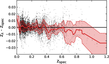
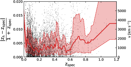
Figure 16: Bias and uncertainty of the photometric cluster redshifts $z_{\lambda}$ estimated by comparing to high quality spectroscopic cluster redshifts $z_{\rm spec}$. Black points refer to 9,522 clusters with high-quality spectroscopic redshifts (see Section 8). The catalogs are merged as described in Section 4.1.1. The red line is the running median, and the red shaded regions give the uncertainty $\delta z_{\lambda}$ taken as the 16^th and 84^th percentiles of the distribution. In the left panel, the continuous red line is the redshift bias $\Delta z_{\lambda}$, and the dashed lines give the redshift uncertainty $\delta z_{\lambda}$. The right panel shows the absolute errors normalized by $1+z_{\rm spec}$, which is proportional to the line-of-sight velocity $v$ (Equation (6)).

Both bias and uncertainty depend on the true redshift $z$: $\Delta z_{\lambda}(z)$ and $\delta z_{\lambda}(z)$. We assume negligible spectroscopic redshift uncertainties $\delta z_{\rm spec}\ll\delta z_{\lambda}$ and zero spectroscopic bias $\Delta z_{\rm spec}=0$, that is, we use $z_{\rm spec}$ as a proxy for the true redshift. The spectroscopic cluster redshifts have, on average, 1$\sim$7 (5$\sim$15) times lower uncertainties than the photometric cluster redshifts when less than 5 (more than 20) spectroscopic members are known.

We estimate the bias and uncertainty by comparing the photometric redshifts $z_{\lambda}$ to the high-quality spectroscopic redshifts $z_{\rm spec}$. By high quality, we mean a minimum number of spectroscopic members to $N_{\rm members}\geq 10$ for $z_{\rm spec}<0.3$, $N_{\rm members}\geq 7$ for $0.3<z_{\rm spec}<0.6$, and $N_{\rm members}\geq 3$ for $z_{\rm spec}>0.6$ To have a sufficient sample size at high redshift, we run eROMaPPer on a large set of test clusters compiled from the works listed in Table 1 and Böhringer et al. (2000); Clerc et al. (2012); Balogh et al. (2014); Paterno-Mahler et al. (2017); Streblyanska et al. (2019); Huang et al. (2020a, b). The test cluster compilation comprises 151,781 clusters distributed across the entire LS area. For a subset of 22,450 clusters, we measure spectroscopic redshifts. We obtain 9,522 clusters with high-quality spectroscopic redshifts to compare the photometric redshift to, see black dots in Figure 16.

We mention as a caveat to these bias and uncertainty estimates that the high-quality spectroscopic sample does not fairly sample the parent cluster sample. There could remain subtle biases that we can only uncover with more spectroscopy or narrow-band photometry. This task can be reassessed once the datasets from SDSS-V (10,000 clusters), 4MOST (40,000 clusters), DESI (DESI Collaboration et al. 2023), and Euclid (Laureijs et al. 2011) become available.

The cosmological analysis in a companion paper (Ghiradini et al. A&A subm.) includes the empirical redshift uncertainties derived in this paper. The bias, however, is not included because it has negligible impact on the inferred cosmological parameters (Ghiradini et al. A&A subm.).

Figure 17: Uncertainties of the eRASS1 photometric cluster redshifts. The black dots are the formal uncertainties $\delta z_{\lambda}^{\rm fml}$ calculated by eROMaPPer as the standard deviation of the redshift posterior $P(z)$. We adopt them as the final redshift uncertainties $z_{\lambda,{\rm err}}$. The dashed red line is the mean of the upper and lower empirical uncertainties $\delta z_{\lambda}^{\rm spec}$ derived from the comparison to the spectroscopic cluster redshifts. The continuous red line is the absolute redshift bias $|\Delta z_{\lambda}|$.

8.1 Redshift Bias

We estimate the redshift bias by applying a running median filter to the points shown in Figure 16:

$$\Delta z_{\lambda}(z)=\underset{z_{\rm spec}\in[z_{\rm min},z_{\rm max})}{\rm median}(z_{\lambda}-z_{\rm spec}),$$ (16)

where the window interval $[z_{\rm min},z_{\rm max})$ is adjusted such that it has a minimum width of $\Delta z=0.02$ and encompasses a minimum of 100 clusters. Each result $\Delta z_{\lambda}$ is assigned to a redshift $z$ of the median $z_{\rm spec}$ in each interval. For the next step, we move the window by $\Delta z=0.01$ from the previous initial redshift $z$. Finally, the data points $\Delta z_{\lambda}(z)$ are linearly interpolated. The result is shown by the continuous red line in Figure 16. It scatters around zero for $0.05<z_{\rm spec}<0.4$ and becomes slightly negative beyond that.

$$\Delta z_{\lambda} ( z_{\rm spec}<0.05) =+0.0040\pm 0.0056,$$

$$\Delta z_{\lambda} (0.05< z_{\rm spec}<0.4) =+0.0004\pm 0.0016,$$

$$\Delta z_{\lambda} (0.4< z_{\rm spec}<0.8) =-0.0041\pm 0.0026,$$

$$\Delta z_{\lambda} (0.8< z_{\rm spec}) =-0.0178\pm 0.0242.$$ (17)

We notice stronger deviations around $z_{\rm spec}=0.4$ (see also Rykoff et al. 2014). Here, the 4000 Å break gets redshifted to the filter transition between the $g$ and $r$ bands. Consequently, neither the $g-r$ nor the $r-z$ color is sensitive to this redshift (see Appendix C). A positive bias just before $z_{\rm spec}<0.4$ and a negative bias just after $z_{\rm spec}>0.4$ creates an artificial clumping of clusters in redshift space at this location (see Figure 12). A similar feature is visible at $z_{\rm spec}=0.7$. Here, the 4000 Å break gets redshifted to the wavelength region between the $r$ and $z$ filters. Nevertheless, the bias remains below $|z_{\lambda}-z_{\rm spec}|<0.01$ for intermediate redshifts $0.6<z_{\rm spec}<0.9$. Beyond $z_{\rm spec}>0.9$, the bias increases to $|z_{\lambda}-z_{\rm spec}|>0.02$. Here, we reach the limiting redshift of the LS (see Figure 3). The colors become less sensitive to redshift (see Appendix C), even though we include the $i$- and $w1$-band magnitudes for the red sequence colors beyond $z_{\lambda}>0.8$. At very low redshifts $z_{\rm spec}<0.05$, the bias increases steeply because the red-sequence model is not calibrated (see Appendix C).

The right panel of Figure 16 shows the absolute deviations $|z_{\lambda}-z_{\rm spec}|$ normalized by $1+z_{\rm spec}$. We find

$$\frac{|z_{\lambda}-z_{\rm spec}|}{1+z_{\rm spec}}\lesssim 0.005 \text{for\leavevmode\nobreak\ \leavevmode\nobreak\ }z_{\rm spec}\lesssim 0.9.$$ (18)

The running median is below or around 0.5% for $z_{\rm spec}\lesssim 0.9$. The previously discussed bias peaks around $z_{\rm spec}=0.4$ and $z_{\rm spec}=0.7$ are apparent here, too.

8.1.1 Small-Scale Patterns in $\Delta z_{\lambda}$

There are small-scale oscillations in photometric redshift bias with an amplitude of $z_{\lambda}-z_{\rm spec}\approx 0.003$ and a period of $\Delta z_{\rm spec}\approx 0.05-0.10$. This is visible as the systematic variations of the red line in Figure 16, left panel. The effect is especially prominent around $z_{\rm spec}\approx 0.4$, where neither the $g-r$ nor the $r-z$ colors are very sensitive to redshift (see Appendix C). The origin of these residuals can be traced back to the red-sequence model calibration. Our tests showed that the amplitude of these oscillations increases when we include the $i$-band in the $z<0.8$ eROMaPPer runs. Even though the statistical uncertainties decrease mildly because more information is being used, the systematic uncertainties increase because of color variations on small scales in redshift space. For this reason, we give higher priority to the $grz$ and $grzw1$ eROMaPPer runs over the runs that include the $i$ band (see Section 4.1.1). In the future, we plan to improve this using finer-spaced spline fitting of the red sequence colors that include the $i$ band.

8.1.2 Average Bias Correction

The photometric redshifts can be corrected for the bias. To do so, we calculate $\Delta_{z}(z_{\lambda})$ instead of $\Delta_{z}(z_{\rm spec})$ because $z_{\lambda}$ is known for every cluster and $z_{\rm spec}$ is only available for a subset. The procedure is equivalent to Equation (16). We compute $\Delta_{z}(z_{\lambda})$ for the subset of clusters with known $z_{\rm spec}$ and subtract it from $z_{\lambda}$ to obtain a bias-corrected photometric redshift $z_{\lambda,{\rm corr}}$:

$$z_{\lambda,{\rm corr}}=z_{\lambda}-\Delta z_{\lambda}(z_{\lambda}).$$ (19)

The corrected redshifts $z_{\lambda,{\rm corr}}$ are provided in the catalog, although all optical cluster properties are calculated at the uncorrected redshifts. As stated in Section 8, the redshift bias has a negligible impact on the inferred cosmological parameters in Ghiradini et al. (A&A subm.).

8.2 Redshift Uncertainties

The formal redshift uncertainty $\delta z_{\lambda}^{\rm fml}$ is calculated by eROMaPPer for each cluster using the standard deviation of the redshift posterior $P(z)$ (see Section 3.2.1). We compare it to an empirical uncertainty $\delta z_{\lambda}^{\rm emp}$ derived from the comparison to spectroscopic cluster redshifts. The empirical uncertainties are calculated as the running 16^th and 84^th percentiles of the $z_{\rm spec}-z_{\lambda}$ distribution. It is analogous to the procedure described in Section 8.1, but we replace the median with the percentiles and subtract the redshift bias to isolate the contribution from the statistical uncertainties. The results for the upper and lower values of $\delta z_{\lambda}^{\rm emp}$ are

$$\delta z_{\lambda}^{\rm emp} ( z_{\rm spec}<0.05) =+0.0093,-0.0078,$$

$$\delta z_{\lambda}^{\rm emp} (0.05< z_{\rm spec}<0.4) =+0.0062,-0.0061,$$

$$\delta z_{\lambda}^{\rm emp} (0.4< z_{\rm spec}<0.8) =+0.0095,-0.0110,$$

$$\delta z_{\lambda}^{\rm emp} (0.8< z_{\rm spec}) =+0.0153,-0.0242.$$ (20)

These uncertainties are relatively small and almost symmetric at low to intermediate redshifts $0.05<z_{\rm spec}<0.4$. Below $z_{\rm spec}=0.05$, the 4000 Å break reaches the blue limit of the $g$ band filter transmission curve, making the $g-r$ color less sensitive to redshift (see Appendix C). In the future, $u$-band data from LSST (Ivezić et al. 2019) will solve this issue. Above $z_{\rm spec}>0.6$, the uncertainties increase because of higher photometric uncertainties for the fainter sources.

The running upper and lower percentiles are also shown in Figure 16, left panel, by the dashed red lines. They confirm the mostly symmetric shape and the increase of $\delta z_{\lambda}^{\rm emp}$ around $z_{\rm spec}\approx 0.7$. That increase happens because the 4000 Å break is redshifted between the $g$ and $r$ filters.

We compare both types of uncertainties in Figure 17. The black points show $\delta z_{\lambda}^{\rm fml}$ for the individual clusters, and the red dashed line is the average of the upper and lower percentiles for $\delta z_{\lambda}^{\rm emp}(z_{\lambda})$. In the range $0.1<z_{\lambda}<0.8$, the empirical uncertainties are consistent with the lower boundary of the formal uncertainties, but individual values for $\delta z_{\lambda}^{\rm fml}$ scatter up. The redshift uncertainty is anti-correlated with richness, so as expected, this happens for poorer clusters with $\lambda\lesssim 10$. Around $z_{\lambda}\approx 0.4$ and $z_{\lambda}\approx 0.7$, both uncertainties increase due to filter transitions. Above $z>0.8$, the formal uncertainties underestimate the empirical uncertainties by a factor of $\approx 2$.

The continuous red line in Figure 17 is the absolute value of the redshift bias evaluated on a grid for $z_{\lambda}$. It is lower than the uncertainties. That is, for an individual cluster, the statistical uncertainty dominates the error budget over the systematic error. We adopt the formal uncertainties, which are calculated by eROMaPPer as the standard deviation of the redshift posterior $P(z)$, as the final photometric redshift uncertainties $z_{\lambda,{\rm err}}=\delta z_{\lambda}^{\rm fml}$ because they also capture the richness dependence. Hence, they are a better estimate of an individual cluster’s redshift uncertainty than the averaged empirical uncertainty for the ensemble.

9 The Richness – Velocity Dispersion Scaling Relation

We investigate the scaling relation between two cluster properties that correlate with cluster mass. The line-of-sight velocity dispersion $\sigma$ traces the dynamical mass $M_{\rm dyn}$ of a cluster

$$M_{\rm dyn}(<r)=c\frac{\sigma^{2}r}{G},$$ (21)

where $G$ is the gravitational constant, $r$ is the cluster radius, and $c$ corrects effects from 2D projection and orbit anisotropy (Binney & Tremaine 2008). The richness $\lambda_{\rm norm}$ also correlates with total cluster mass (e.g., McClintock et al. 2018) because deeper gravitational potential wells attract more baryonic matter.

To correct for redshift evolution, we multiply $\lambda_{\rm norm}$ with $E(z)=\sqrt{\Omega_{\rm m}(1+z)^{3}+\Omega_{\lambda}}$ (Damsted et al. 2023), although the effect is small. Most spectroscopic cluster sample is at low redshift (see Figure 5). We explore the $\sigma-\lambda_{\rm norm}$ relation for the eRASS1 sample augmented by the literature samples. The scaling relation between X-ray, weak lensing, and optical observables are detailed in companion papers (Ghiradini et al. A&A subm.; Grandis et al. A&A subm.; Pacaud in prep.).

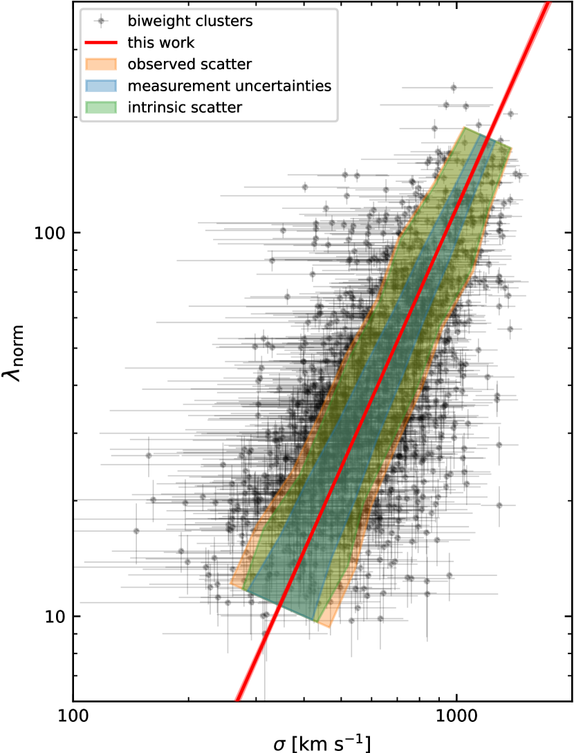
Figure 18: Relation for cluster line-of-sight velocity dispersion $\sigma$ and richness $\lambda_{\rm norm}$. The black data points are for all clusters in our analyzed catalogs (see Table 4) apart from the blind-mode runs. In total, 1,699 clusters with $N_{\rm members}\geq 15$ spectroscopic members are selected. The red line is the best fit to the data, and the light red shades show the uncertainty of the relation. The observed scatter $\delta_{\rm obs,orth}$ (orange) is measured orthogonal to the best-fit relation in 9 bins. The median orthogonal component of the measurement uncertainties $\delta_{\rm m,orth}$ is shown for each bin in blue. By subtracting $\delta_{\rm m,orth}$ from $\delta_{\rm obs,orth}$ in quadrature, we estimate the intrinsic scatter $\delta_{\rm in}$ for each bin. It is shown in green.

9.1 Cluster Selection

For the analysis, we consider only clusters with high-quality (unflagged) velocity dispersions determined using the bi-weight scale estimator (see Section 3.6). As we require a large number of $\geq 15$ spectroscopic members for this method, these clusters also have a high richness and a low relative uncertainty: $\delta\sigma/\sigma\sim 20\%$. We show how these clusters populate the $\sigma-\lambda_{\rm norm}$ plane in Figure 18. The Figure contains data for 1,699 clusters with a low masking fraction of $<20\%$. Of them, 309 are eRASS1 clusters.

We assume that sample selection effects are unimportant for this analysis. For eRASS1, the X-ray count rate is the primary selection variable. For a thin redshift slice, the velocity dispersion and the richness correlate with the X-ray count rate. Hence, the net selection effect is along the relation and, therefore, unimportant when applying orthogonal distance regression.

9.2 Relation Fitting

We fit a linear relation with free parameters $\alpha$ and $\beta$ to the logarithm of both variables;

$$\log(\lambda_{\rm norm})=\alpha\times\log(\sigma[{\rm km\,s^{-1}}])+\beta.$$ (22)

Our preferred fitting method (ODR, Boggs et al. 1989) minimizes the orthogonal residuals from the relation. Additionally, we weigh the individual data points by their measurement uncertainties in both variables and include the non-negligible intrinsic scatter. The method is described in detail in Kluge & Bender (2023). An advantage is that the method is insensitive to switching variables.

The best-fit values are

$$\alpha =\phantom{-}2.401\pm 0.055,$$ (23)

$$\beta =-5.074\pm 0.156,$$ (24)

with a covariance of COV$(\log\lambda_{\rm norm},\log\sigma)=-8.6\times 10^{-3}$. Our best-fit slope agrees within 1.5$\sigma$ confidence with $\alpha=1/(0.323\pm 0.057)=3.10^{+0.66}_{-0.46}$ obtained by Kirkpatrick et al. (2021). The agreement improves to 0.8$\sigma$ ($\alpha=2.734\pm 0.082$) confidence when we use the same fitting method (BCES, Akritas & Bershady 1996; Nemmen et al. 2012).

Moreover, our best-fit slope also agrees within 1.6$\sigma$ confidence with $\alpha=1/(0.365\pm 0.029)=2.74^{+0.23}_{-0.20}$ obtained by Damsted et al. (2023). However, their applied fitting method linmix (Kelly 2007) is sensitive to switching variables. Using that method, we get consistent results only for $(\sigma|\lambda_{\rm norm})$: $1/\alpha=0.392\pm 0.010$. For $(\lambda_{\rm norm}|\sigma)$, we get $\alpha=1.753\pm 0.045$, a 9$\sigma$ deviation.

The statistical uncertainties of the best-fit slopes improve by a factor of 4–10 compared to previous works. This is attributed to the large gain in sample size of clusters with $N_{\rm members}\geq 15$ spectroscopic members. Our sample includes 1,699 clusters compared to 530 clusters (Damsted et al. 2023). The sample of (Kirkpatrick et al. 2021) includes 2740 clusters but with a lower median of 10 spectroscopic members.

9.3 Intrinsic Scatter

We estimate the intrinsic scatter following the procedure in Kluge & Bender (2023). First, we calculate the observed orthogonal scatter $\delta_{\rm obs,orth}$ and the median orthogonal component of the measurement uncertainties $\delta_{\rm m,orth}$. Then, the intrinsic scatter $\delta_{\rm in}$ can be estimated by

$$\delta_{\rm in}=\sqrt{\delta^{2}_{\rm obs,orth}-\delta^{2}_{\rm m,orth}}.$$ (25)

To capture a possible variation with $\sigma$ or $\lambda_{\rm norm}$, we split the sample into 9 equal-sized bins perpendicular to the best-fit line. In each bin, we calculate $\delta_{\rm obs,orth}$, $\delta_{\rm obs,orth}$, and $\delta_{\rm in}$, and show results in Figure 18 by the orange, blue, and green shades, respectively. Notably, not only do the measurement uncertainties increase for the lower $\sigma$ or $\lambda_{\rm norm}$, as expected, but also the intrinsic scatter increases.

We report the obtained values for two larger bins, split at $\sigma=620$ km s^-2 and $\lambda_{\rm norm}=43$. For the subsample at high $\sigma$ and $\lambda_{\rm norm}$, we obtain $\delta_{\rm obs,orth}=0.100$ dex, $\delta_{\rm m,orth}=0.039\pm 0.026$ dex, and $\delta_{\rm in}=0.092\pm 0.008$ dex. For the subsample at low $\sigma$ and $\lambda_{\rm norm}$, we obtain $\delta_{\rm obs,orth}=0.118$ dex, $\delta_{\rm m,orth}=0.058\pm 0.029$ dex, and $\delta_{\rm in}=0.102\pm 0.012$ dex. This is slightly lower than $\delta_{\rm in}=0.138\pm 0.017$ obtained by Damsted et al. (2023), possibly because we apply different fitting and scatter-estimation methods. We conclude that the $\sigma-\lambda_{\rm norm}$ relation obtained in this work is dominated by intrinsic scatter and not by measurement uncertainties.

10 Summary

The first eROSITA All-Sky Survey (eRASS1) provides the largest sample of ICM-selected galaxy clusters and groups in the western galactic hemisphere to date. In this work, we have identified 12,247 candidates by associating them with a coincident overdensity of red-sequence galaxies or, in 247 cases, by matching them with known clusters from the literature. We have run the red-sequence-based cluster finder eROMaPPer on optical and near-infrared data from DESI Legacy Imaging Surveys DR9 (at Decl. $>32.375\degr$) and DR10 (at Decl. $<32.375\degr$) on 13,116 deg² of the sky. The eRASS1 sample of cluster and group candidates is designed to be as complete as possible. After discarding candidates without optical identification, we estimate the purity using a mixture model to be 86%.

We provide optical (redshifts, richnesses, optical centers, BCG position) and spectroscopic (redshifts and velocity dispersions) properties. The photometric redshifts have an excellent accuracy of $\Delta z/(1+z)\lesssim 0.005$ for $0.05<z<0.9$. For individual clusters, the accuracy is dominated by statistical uncertainties.

Spectroscopic redshifts are calculated for a subsample of 3210 eRASS1 clusters and groups. Of those, 1759 have at least three spectroscopic members. The spectroscopic galaxy redshifts are compiled from public catalogs from the literature and dedicated follow-up programs and matched to the photometrically selected member galaxies. The spectroscopic cluster redshifts are, on average, 1$\sim$7 (5$\sim$15) times more accurate than the photometric cluster redshifts when less than 5 (more than 20) spectroscopic members are known. This improvement in accuracy makes the eRASS1 clusters align well with the large-scale structure as traced by individual spectroscopic galaxy redshifts.

Velocity dispersions are measured for 1,906 clusters, of which 1,499 are robust, and 358 have high quality with relative uncertainty $\delta\sigma/\sigma\approx 20\%$.

In addition to the eRASS1 catalog, we consistently remeasured the redshifts on known clusters from the literature. We recover consistent redshifts in the range $0.05\lesssim z\lesssim 1.1$ for $>95\%$ of the clusters detected with the high-$z$-sensitive Sunyaev-Zeldovich effect or low-$z$-sensitive optical selection. The outliers are explained by multiple structures coinciding along the line of sight.

Moreover, we detect galaxy clusters without positional priors in the full footprint of the Legacy Surveys (24,069 deg²). The number density of the found clusters is independent of the optical survey depth below the local limiting redshift $z_{\rm vlim}$. The depth of the LS limits the high-quality subsample at around $z_{\rm vlim}\approx 0.7$ for a minimum galaxy luminosity of 0.2 L_∗. By increasing the luminosity threshold to $L>0.4$ L_∗ and including the $i$ and $w1$ filter bands, we increase the limiting depth to $z_{\rm vlim}\approx 1.0$ and even higher locally.

Combining all analyzed cluster catalogs, we obtain a sample of 1,699 clusters with high-quality velocity dispersion measurements. We correlate it with the richness and find a best-fit relation $\log(\lambda_{\rm norm})=2.401(\pm 0.055)\times\log(\sigma[{\rm km\,s^{-1}}])-5.074(\pm 0.156)$, which agrees with previous results from other studies. The scatter in the relation is dominated by an intrinsic scatter $\delta_{\rm in}$ for the full range $300\lesssim\sigma\lesssim 1000$ km s^-1 and $10\lesssim\lambda\lesssim 200$. It increases only slightly from $\delta_{\rm in}=0.092\pm 0.008$ dex to $\delta_{\rm in}=0.102\pm 0.012$ dex toward lower $\sigma$ and $\lambda$.

In the future, the next-generation eROSITA cluster catalogs will be supported by a wealth of spectroscopic input from SDSS-V (10,000 clusters), 4MOST (40,000 clusters), LSST, and Euclid. These data will expand bias-free redshift measurements to higher redshifts. A complete sampling of the nodes of the cosmic web will yield exquisite constraints on cosmological models and primordial non-Gaussianity (Stopyra et al. 2021).

Data Availability

We make available the optical properties of the eRASS1 galaxy cluster and group catalog. Moreover, the measured optical properties of the clusters from literature catalogs and eROMaPPer runs without positional priors are made available, too. Reasonable requests for the member galaxy catalogs can be made to the corresponding author.

Appendix A Limitations & Caveats

This section gives a concise overview of the limitations of the eRASS1 cluster and group catalog. It is important for the user to understand the caveats in order to avoid unnecessary confusion.

A.1 Completeness

The optical completeness decreases at low redshift $z<0.05$ because we discard galaxies that overlap with large galaxies (see Sections 2.2.3 and 5.3). This affects especially clusters or groups that host a cD galaxy. At high redshifts, the catalog is almost complete for high cluster masses and is mostly limited by the depth of the LS. It is quantified by the parameter $z_{\rm vlim}$ (see Appendix B). If a cluster is found at a higher redshift $z_{\lambda}>z_{\rm vlim}$, the probability increases that the detection is a contaminant (see Figure 13). We advise the user to avoid these clusters and select a clean sample using the boolean catalog parameter IN_ZVLIM.

Our cluster finder is based on the colors of galaxies, which follow the red sequence. Hence, star-forming late-type galaxies cannot be part of our member galaxy sample. To confirm this, we run eROMaPPer on the Hickson compact group catalog (Hickson 1982), which consists mostly of low-$z$ late-type galaxies. We recover 17/100 groups that consist of mostly early-type galaxies at $z_{\lambda}<0.1$. The remaining 83/100 groups are not detected by eROMaPPer, as expected.

A.2 Contamination Estimates for Galaxy Groups

Our contamination estimator (see Section 7) seems to perform well at assigning a high contamination probability $P_{\rm cont}$ to possible AGN for high X-ray count rates and low richnesses (see Figure 15, right panel, top left projection). However, sources with low X-ray count rates always receive $P_{\rm cont}\approx 0$. These count rates occur during the multi-component fitting using MBproj2D (see Bulbul et al. A&A subm.). They are not part of the expected count rates for random sky points. Hence, the kernel density estimate for this region in parameter space is almost zero for the contaminants. Consequently, our contamination estimator underestimates the true contamination on the galaxy group scale.

In contrast, visual inspection of real groups ($\lambda_{norm}\lesssim 10$) at low redshift ($z_{\rm best}\lesssim 0.1$) reveals that many of them receive a high $P_{\rm cont}$ value. In principle, lowering the member luminosity threshold below $L<0.2$ L_∗ can help distinguish them better from AGN. This would increase the measured richnesses of real groups while we expect the richnesses of AGN to remain low.

A.3 Cluster Properties

The cluster parameters are always calculated at the photometric redshift $z_{\lambda}$. This concerns the galaxy memberships, richnesses $\lambda$ and $\lambda_{\rm norm}$, optical centers, and velocity dispersions $\sigma$. In cases where the best redshift type was changed to a literature redshift, the cluster parameters are not reliable because they refer to a foreground or background cluster.

A.4 Masked Clusters

Few clusters have a large mask applied, which covers roughly one-half of their extent. One example is 1eRASS J022553.0-415457 with a masking fraction of 40%. We notice that we detect member galaxies only on the other side of this cluster when we run eROMaPPer on a position that falls within the initial mask. That means, the mask was not created based on flagged photometry in the LS. We suspect that it occurs when a cluster is located at an edge of a heal pixel. Nevertheless, the richnesses are corrected for the masking fraction (see Section 3), and hence, they are noisier but unbiased. Also, we have no reason to assume that the photometric redshifts would be biased in the described cases. Moreover, only a small fraction of the eRASS1 clusters is affected. Four percent of them have a masking fraction of $>40\%$ and for most of them, a saturated nearby star is the reason for the mask.

A.5 Velocity Dispersion

We provide cluster velocity dispersions even when the velocity clipping diverged in some of the bootstrapped samples (see Section 3.6). This affects 407 out of 1906 cases that can be identified by the flag VDISP_FLAG_BOOT¿0. Two examples with the unrealistically high velocity dispersions $\sigma>10,000$ km s^-1 are 1eRASS J104344.4+240537 and 1eRASS J025101.7-353415. In both cases, the velocity dispersion is high because one wrongly measured redshift around $z_{\rm spec}=0$ was not clipped. This error is taken into consideration in the uncertainty $\delta\sigma>10,000$ km s^-1, which is almost equal to $\sigma$ itself. The spectroscopic redshifts are less affected by these outliers because the biweight location for the spectroscopic cluster redshifts happens to be more robust than the gapper estimator for the velocity dispersion.

A.6 Bias-Corrected Photometric Redshifts

Red-sequence model calibration errors (see Section C) propagate to biases in the photometric cluster redshifts (see Section 8.1). We have measured this bias and provide corrected photometric redshifts $z_{\lambda,{\rm corr}}$ (see Equation (19)) and corresponding uncertainties. These corrections are small at low redshifts but become increasingly important at $z\gtrsim 0.8$. In particular, the formal uncertainties underestimate the real uncertainties significantly at $z\gtrsim 0.8$.

Appendix B Limiting Depth and Limiting Redshift

LS DR10 south
 

 
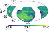
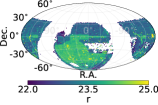
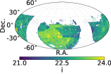
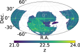
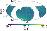
LS DR9 north
 
                               

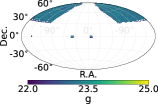
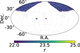
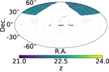
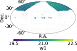
Figure 19: Depth maps showing the limiting magnitude for the Legacy Surveys DR10 south (top panels) and DR9 north (lower panels) in different filter bands. The maps present the full coverage in each band independently rather than combining the footprints as in Figure 2. The limiting magnitude is defined as the brightness of a galaxy whose flux has a signal-to-noise ratio of 10.

To minimize the number of spurious sources, it is necessary to know whether the local survey depth is sufficiently deep. This information is stored in depth maps. The sky position-dependent depth is estimated via a parametric model (Rykoff et al. 2015) that uses the galaxy magnitudes and uncertainties in the LS. The limiting magnitude is defined by that of a galaxy with a detection confidence of 10$\sigma$, that is, its measured flux has a signal-to-noise ratio of 10. These limits vary across the sky and for different filter bands. Depth maps store this information in the HEALPix format (Górski et al. 2005). We use a spatial resolution of NSIDE=4096, which corresponds to an area of $\leavevmode\nobreak\ \sim 1\arcmin\times 1\arcmin$ per pixel. If a heal pixel contains an insufficient number of galaxies for the model to converge, the depth is approximated by recursively expanding out to the next largest pixel in the nested scheme until it does.

One depth map is created for each filter band and for each of the LS DR10 south and LS DR9 north survey parts (see Figure 19). Their spatial coverage is similar but not identical. Therefore, we set all heal pixels to empty which are also empty in at least one of the depth maps used in each eROMaPPer run. The resulting $z$-band depth map for the $grz$ filter band combination is shown in Figure 2. The top panel refers to the LS DR10 south and the bottom panel refers to the LS DR9 north.

Saturated sources leave small holes in the depth maps. If a cluster center is located within such a hole, we describe it as formally outside of the footprint and mark it in the catalog as IN_FOOTPRINT=False. Part of the cluster can still be detected when the cluster radius $R_{\lambda}$ is larger than the size of the masked region. This affects 363 eRASS1 clusters. We show one example in Figure 20. A bright foreground star overlaps with a cluster in the background. The galaxies in projected proximity have flagged photometry in the LS. They are rejected by eROMaPPer (see Section 3). However, cluster members in the outskirts of the cluster are still detected and marked by the circles. As expected, the masking fraction is high with MASKFRAC=0.51, and therefore, the richness $\lambda$ is upscaled by a factor of SCALEVAL=2.03. We consider the photometric redshift $z_{\lambda}=0.400\pm 0.012$ reliable because 45 member galaxies are detected despite the high masking fraction. For this reason, we keep these clusters in our sample.

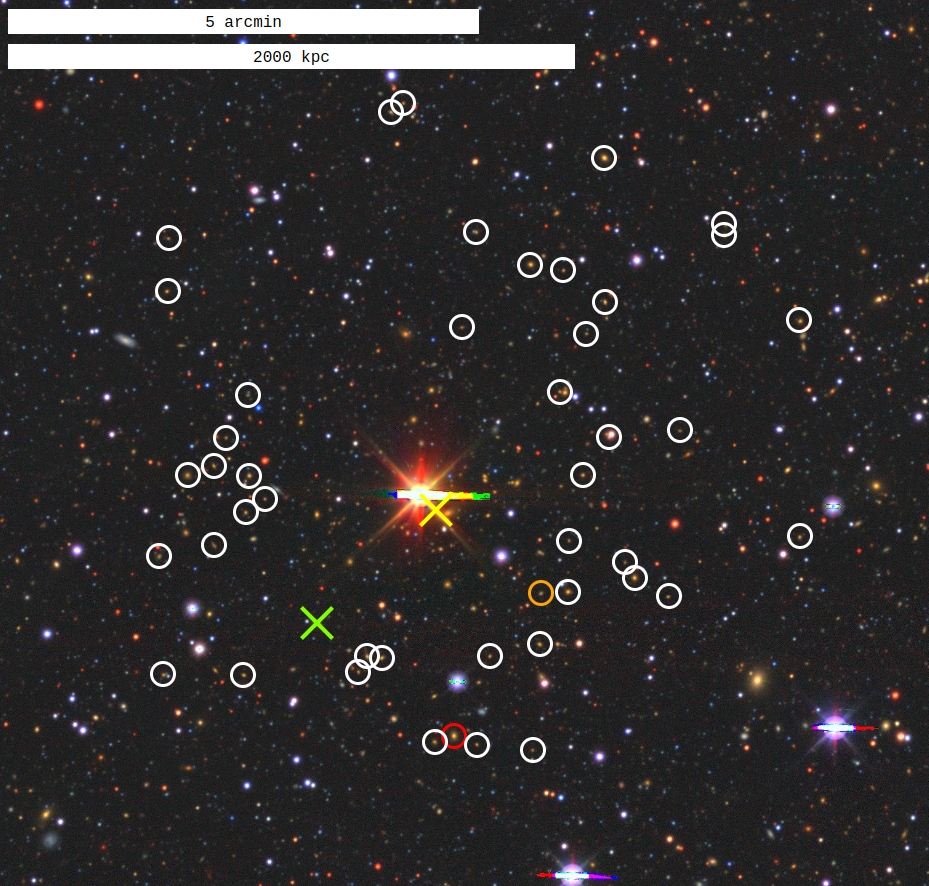
Figure 20: Example of a cluster 1eRASS J010123.5-764801 that is located in a masked area of the footprint map. The saturated foreground star near the X-ray detection (yellow cross) is responsible for the mask. Cluster member galaxies are marked by circles (see Figure 4 for further descriptions of the labels). Only the members in the outskirts of the cluster are identified. North is up, east is left.

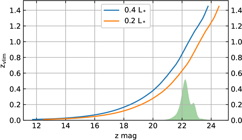
Figure 21: Conversion from limiting $z$-band magnitude to limiting redshift $z_{\rm vlim}$ for galaxies with a luminosity $L=0.2$ L_∗ (orange) and $L=0.4$ L_∗ (blue). Restricting the sample to brighter members allows for probing higher redshifts. For reference, the green histogram shows the distribution of limiting magnitudes in the $z$ band for the combined full LS DR10 south and LS DR9 north areas.

The limiting magnitude in our reference band, the $z$ band, can be converted to a limiting redshift $z_{\rm vlim}$ for non-empty heal pixels. It is defined as the redshift, at which a member galaxy at the low-luminosity limit $L_{\rm thresh}$ can still be detected with a 10$\sigma$ significance. To calculate this limit, we predict the brightness in the DECam $z$ band of a galaxy with luminosity $L_{\rm thresh}$ for all redshifts $0.01<z<1.45$ using the tool EzGal (Mancone et al. 2013). Thereby, we assume that it behaves according to the prediction for a passively evolving single stellar population (Bruzual & Charlot 2003). We set the low-luminosity limit to $L_{\rm thresh}=0.2$ L_∗ for the eROMaPPer runs using the $grz$ and $griz$ filter bands, and $L_{\rm thresh}=0.4$ L_∗ for the runs that include the $w1$ band (see Section 4.1.1 and Figure 21). Hereby, L_∗ is the luminosity at the break of the Schechter function (Schechter 1976). The magnitude of an L_∗ galaxy is normalized to 17.85 $i$ mag in the Sloan photometric system at redshift $z=0.2$, consistently to Rykoff et al. (2016).

Our choice to base the largest reliable redshift purely on the $z$ band deviates from Rykoff et al. (2016) who use a combination of the limiting magnitudes in every filter band to calculate a maximum redshift $z_{\rm max}$. We have shown that the cluster number density remains unbiased for clusters $z_{\lambda}<z_{\rm vlim}$ (see Figure 13). As $z_{\rm max}<z_{\rm vlim}$, this allows us to probe even higher redshifts. We emphasize that we do not discard clusters with higher than the limiting redshift $z_{\lambda}>z_{\rm vlim}$. They are kept in the catalogs with a flag IN_ZVLIM=False.

Appendix C Red Sequence Models

Photometric redshifts are calculated by comparing the galaxy colors to a spline-based red-sequence model (Rykoff et al. 2014). The color–redshift relations for the red-sequence model must be calibrated with the colors of red galaxies with known spectroscopic redshifts. For this, we utilize our spectroscopic galaxy redshift compilation (see Section 2.3 and Appendix D). As explained in Section 4.1.1, we run eROMaPPer six times using different filter band combinations. The red-sequence model is calibrated for each run independently, corresponding to the six rows in Figure 22.

We begin the model fitting procedure by assuming an initial red-sequence model, which is derived from the predictions of a passively evolving single stellar population (Bruzual & Charlot 2003). We then select red galaxies whose colors are consistent with the initial model. Figure 22 shows the color-coded point density of the final sample for each photometric color.

The spline nodes of the red-sequence model (red points) are then fitted to the colors in redshift bins. Outliers are iteratively clipped. We choose a small node spacing of $\Delta z_{\rm spec}=0.05$ for the $grz$ and $griz$ filter band combinations to capture high-frequency color variations. If not well fitted, systematic residuals lead to a higher local redshift bias (see Section 8.1), which in turn leads to local clumping of the cluster number densities (see Figure 12). A larger node spacing of $\Delta z_{\rm spec}=0.10$ is applied for the $grizw1$ and $grzw1$ filter band combinations. This is better suited for the red-sequence model calibration for the high-redshift ($z_{\lambda}>0.8$) eROMaPPer runs because the number of training galaxies becomes low.

The minimum redshift of the model is $z_{\rm spec}=0.05$. The maximum redshift is $z_{\rm spec}=0.9$ for the $grz$ and $griz$ filter band combinations and $z_{\rm spec}=1.2$ for the $grzw1$ and $grizw1$ combinations. Including the near-infrared $w1$ band helps to constrain better cluster redshifts at $z>0.8$ because the $z-w1$ colors have a non-negligible slope. However, it not necessarily helps for low$-z$ cluster redshifts because of the relatively large scatter of the $z-w1$ colors. For this reason and the more uncertain photometry in the $w1$ band (see Section 2.2), we do exclude it for the low$-z$ eROMaPPer runs.

As mentioned previously, photometric redshifts are calculated by comparing the galaxy colors to the red-sequence model. Thereby, all filter bands are taken into account at all redshifts. Figure 22 confirms that different filter bands are suited better or worse to constrain specific redshift intervals. The higher the slope of the color–redshift relation, the better the color constrains the redshift. Hence, each color is weighted by the local slope of its color–redshift relation.

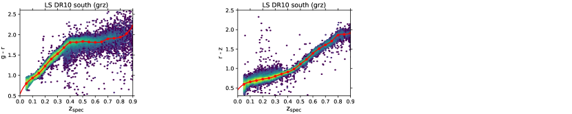
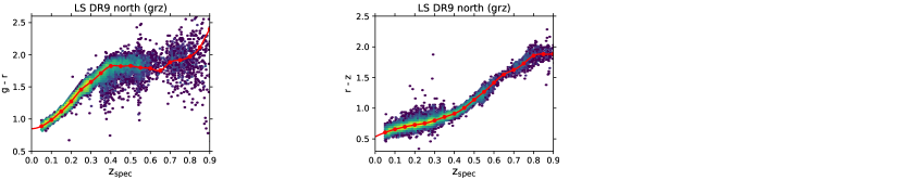
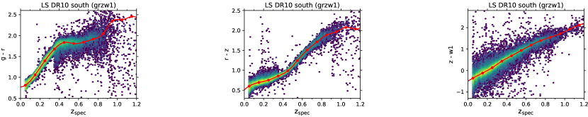
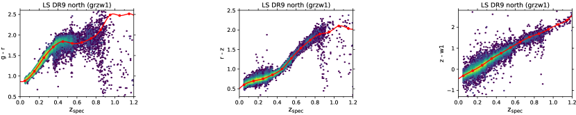
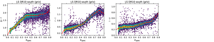
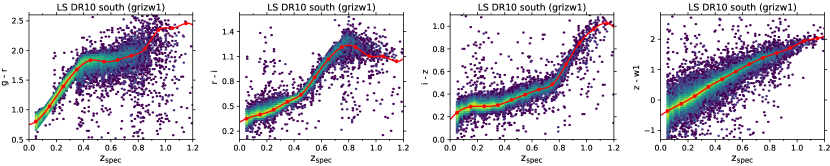
Figure 22: Red-sequence models for the six different calibrations (rows). Each filter band combination and LS parts are labeled in the titles of the subpanels. The combination of $n$ filter bands allows for red-sequence models in $n-1$ colors (columns). The red-sequence models are shown by the red splines and red points mark the spline nodes. The training galaxies are color-coded according to their point density. Their total numbers are, after clipping, $\sim$93,000 for LS DR10 ($grz$ and $grzw1$), $\sim$72,000 for LS DR10 ($griz$ and $grizw1$), and $\sim$36,000 for LS DR9 north ($grz$ and $grzw1$).

Appendix D Details about the Spectroscopic Galaxy Redshift Compilation

The sources, number of entries, and query commands are listed for the spectroscopic galaxy redshift compilation in Table 5. The distribution of all redshifts is shown in Figure 23.

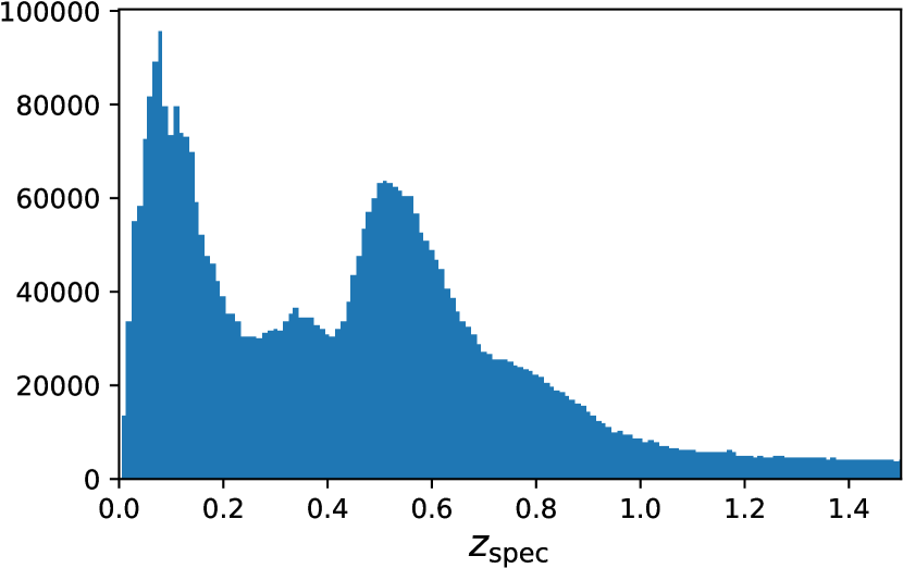
Figure 23: Redshift distribution of the spectroscopic galaxy redshift compilation.

Source	# Galaxies	Query
Abolfathi et al. (2017)	900	in_DESComplilation and des_flags ¿= 3
Aguado-Barahona et al. (2019)	21
Agulli et al. (2016)	430
Ahumada et al. (2020)	450130	zwarning == 0 and z ¿ z_err and z_err ¿ 0
Alam et al. (2015)	933644	zWarning == 0
Almeida et al. (2023)	5034	zwarning == 0 and z ¿ z_err and z_err ¿ 0
		and survey == ”BHM” and plug_ra != 0
Amodeo et al. (2018)	10
Bacon et al. (2023)	37
Balogh et al. (2014)	29	q_z ¿= 3 and Class == ”p ”
Balogh et al. (2020)	507	member == 1 and Redshift_Quality ¿ 2 and Spec_Flag ¡ 2
Balzer et al. (in prep)	154
Bayliss et al. (2011)	26
Bayliss et al. (2016)	1655
Bayliss et al. (2017)	1578
Bezanson et al. (2018)	99
Blake et al. (2016)	53534	in_DESComplilation and des_flags ¿= 3
Bradshaw et al. (2013); McLure et al. (2013)	1296
Caminha et al. (2017)	3448	q_z ¿ 2
Caminha et al. (2019)	451	z ¿ 0 and (q_z == 2 or q_z == 3)
Carrasco et al. (2017)	730
Castagné et al. (2012)	92
Castignani et al. (2020)	5
Cava et al. (2009)	2686	Mm == 1
Childress et al. (2017)	11264	flag !=6
Clerc et al. (2020)	27783	z ¡ 0.6 and screen_ismember_w ¿ 0.5
Coe et al. (2012)	165	Mm == 1
Coil et al. (2011); Cool et al. (2013)	168546	ZQUALITY ¿= 3 and not a star
Colless et al. (2001)	165911	q_z ¿= 3
Connelly et al. (2012)	4566
Connor et al. (2019)	26	q_z == 3
Cooper et al. (2012)	4366	Q ¿= 3
Crawford et al. (2011)	585	q_z ¿= 2
Czoske et al. (2001)	382	q_z == ”A” or q_z == ”B”
Davis et al. (2003, 2007)	4	in_DESComplilation and des_flags ¿= 3
Davis et al. (2003); Newman et al. (2013)	20022	ZQUALITY ¿= 3 and not a star
Dawson (2013)	688
Deger et al. (2018)	167	Set == ”C” or Set == ”G”
Demarco et al. (2005)	24
Demarco et al. (2007)	33
Demarco et al. (2010)	30
Deshev et al. (2017)	189	Memb == 1
Dressler et al. (1999)	144	Mm == ”c”
Drinkwater et al. (2010)	21656	Qop¿=4
Driver et al. (2011)	48875	in_DESComplilation and des_flags ¿= 3
Ebeling et al. (2014)	1589
Ebeling et al. (2017)	82
Eisenhardt et al. (2008)	76
Ferrari et al. (2003)	105	q_cz == 1
Foëx et al. (2017)	738	EZflag ¿ 0 and zspec ¿ 0
Foley et al. (2011)	12
Fossati et al. (2019)	71	Redshift ¿ 0
Garilli et al. (2008); Le Fèvre et al. (2004)	359	in_DESComplilation and des_flags ¿= 3
Garilli et al. (2014)	44103	2.6¡flag¡4.6, 22.6¡flag¡24.6 (secondary),
		12.6¡flag¡14.6 (broad-line AGN),
		212.6¡flag¡214.6 (broad-line AGN, secondary)
Garilli et al. (2021)	146	zflg == 3 or zflg == 4
Geha et al. (2017)	15313	in_DESComplilation and des_flags ¿= 3
George et al. (2011)	2033
Girardi et al. (2010)	126
Golovich et al. (2019)	3061
Gómez et al. (2012)	40

Gonzalez et al. (2019)	1
Gschwend et al. (2018)	7156	in_DESComplilation and des_flags ¿= 3
Guennou et al. (2014)	69
Guglielmo et al. (2018)	1888	q_z == 400 and DRr200_1 ¿ 0
Haines (2021)	10895	CL == 1
Halliday et al. (2004)	72
Hansen et al. (2002)	36	Note == ”b” and u_z != ”:” and u_z != ”::”
Hilton et al. (2020)	726	redshiftType == ”spec”
Huchra et al. (2012)	13375	n_cz != ”S” and n_cz != ”6”
Hwang et al. (2014)	4142
Inami et al. (2017)	346	Confid ¿ 1
Jones et al. (2009)	93437	q_z == 4
Jørgensen et al. (2014)	10	Mm == 1
Jørgensen et al. (2017)	71
Karman et al. (2015)	31
Khabibullina & Verkhodanov (2009)	1478
Khullar et al. (2018)	34
Kirk et al. (2015)	107	Memb == ”V”
Kluge et al. (2020)	90
Koranyi & Geller (2002)	225
Le Fèvre et al. (2013)	32288	flag=3, 4, 22, 24 (2xs are secondary),
		13, 14 (broad-line AGN),
		213, or 214 (broad-line AGN, secondary)
Lee et al. (2019)	50	flag != ”star” and Cluster_ID != ”-99999”
Lemze et al. (2013)	1598
Lidman et al. (2016)	3066	in_DESComplilation and des_flags ¿= 3
Lidman et al. (2020)	894	Object_types.str.contains(”luster”)
Lilly et al. (1995)	381	Class ¿= 3
Lilly et al. (2009)	12870	Flag 4s, 3s, 2.5, 2.4, 1.5, 9.5, 9.4, 9.3 are considered secure
Liske et al. (2015)	41261	NQ¿=4
Liu et al. (2012)	6
Liu et al. (2018)	47	Mm == ”Y”
Mao et al. (2012)	524	in_DESComplilation and des_flags ¿= 3
Masters et al. (2017, 2019)	3092
Maturi et al. (2019)	7470	prob ¿ 0.8 and has_spec_z
McClintock et al. (2018)	654	Z_SPEC ¿ 0 and P ¿ 0.9
McDonald et al. (2016)	29
McLure et al. (2017)	85	q_zsp ¿ 2
Mirkazemi et al. (2015)	3
Momcheva et al. (2016)	31043	in_DESComplilation and des_flags ¿= 3
Moran et al. (2005)	87
Moretti et al. (2017)	7014	Memb ¿= 1
Morris et al. (2007)	279
Muzzin et al. (2009)	25
Muzzin et al. (2012)	217	in_DESComplilation and des_flags ¿= 3
Nanayakkara et al. (2016)	40	in_DESComplilation and des_flags ¿= 3
Nastasi et al. (2014)	108
Nilo Castellón et al. (2014)	79
Oguri et al. (2018)	753	z_spec ¿ 0
Olsen et al. (2003)	128	Memb == ”m”
Olsen et al. (2005)	266
Owen et al. (1995)	65
Owers et al. (2011)	2350
Parkinson et al. (2012)	8	in_DESComplilation and des_flags ¿= 3
Pierre et al. (1997)	4
Pierre et al. (2016)	51
Pimbblet et al. (2006)	5015
Postman et al. (2001)	12	(f__PLO2001_ == ” *” or f__PLO2001_ == ”* ” or
		f__PLO2001_ == ”*” or f__PLO2001_ == ”**”)
		and q_z ¿= 2
Pranger et al. (2014)	139
Psychogyios et al. (2020)	23	m == 1

Rescigno et al. (2020)	27	QF ¿ 1
Rest et al. (2014); Scolnic et al. (2014); Kaiser et al. (2010)	1128	in_DESComplilation and des_flags ¿= 3
Ricci et al. (2018)	111	flag == ”s”
Richard et al. (2021)	1271	zconf ¿ 1
Rines et al. (2000)	153
Rines et al. (2016)	2603	Mm == 1
Rines et al. (2018)	2929	Mm == 1
Robotham et al. (2011)	32361	GroupID != 0
Rudnick et al. (2017)	104	Env == ”cluster” or Env == ”group”
Ruel et al. (2014)	948
Runge & Yan (2018)	126	zspec ¿ 0
Rykoff et al. (2012)	9353	zsp ¿ 0
Rykoff et al. (2016)	28950	zspec ¿ 0 and PMem ¿ 0.9
Schirmer et al. (2011)	36	Mm == ”b”
Shectman et al. (1996)	8862
Sifón et al. (2013)	219
Silverman et al. (2015)	450	flag ¿= 3
Skelton et al. (2014); Momcheva et al. (2016)	6644	z_best_s = 2
Sluse et al. (2019)	59	Type == ”E”
Smith et al. (2000)	94
Sohn et al. (2018b)	2013	Mem == ”Y”
Sohn et al. (2018a)	762
Sohn et al. (2019a)	152	Mem == ”Y” and BCG == ”Y”
Sohn et al. (2019b)	877
Sohn et al. (2020b)	14388
Sohn et al. (2020a)	131
Song et al. (2017)	48	Mm == 1
Stanford et al. (2014)	171
Stanford et al. (2021)	568
Stott et al. (2008)	52
Straatman et al. (2018)	1195	Use == 1
Strait et al. (2018)	15	QF == ”3” or QF == ”4”
Streblyanska et al. (2019)	17
Sullivan et al. (2011)	243	in_DESComplilation and des_flags ¿= 3
Tanaka et al. (2009)	89	q_z == 0
Tasca et al. (2017)	139	in_DESComplilation and des_flags ¿= 3
Tran et al. (2007)	41	q_z ¿ 1
Treu et al. (2015)	603	in_DESComplilation and des_flags ¿= 3
Verdugo et al. (2008)	143	Memb != ”field”
Wen & Han (2018)	1927
Willis et al. (2013)	21
Wilson et al. (2016)	3005
Yang et al. (2018)	2993
Zaznobin et al. (2020)	27
Zeimann et al. (2013)	7	abs(__z_ - z) ¡ 0.001
Zou et al. (2019) (compilation)	2470093
total	4,882,137

Table 5: Overview of the spectroscopic galaxy compilation that is used to calibrate the red sequence models, and calculate spectroscopic cluster redshifts and velocity dispersions. The individual references are given in column (1). Column (2) provides the number of unique galaxy redshifts from each reference that went into the compilation. The queries in column (3) are the applied selections. Please note that the Zou et al. (2019) source is a compilation of several spectroscopic surveys: 2dFGRS (Colless et al. 2001), 2SLAQ (Cannon et al. 2006), 6dFGS (Jones et al. 2004, 2009), CFRS (Lilly et al. 1995), CNOC2 (Yee et al. 2000), DEEP2 (Davis et al. 2003; Newman et al. 2013), SDSS DR14 (Abolfathi et al. 2018), VIPERS (Garilli et al. 2014; Guzzo et al. 2014), VVDS (Le Fèvre et al. 2005; Garilli et al. 2008), WiggleZ (Drinkwater et al. 2010; Parkinson et al. 2012), and zCOSMOS (Lilly et al. 2007).

Appendix E Catalog Column Descriptions

Table 6 gives an overview of the column names, data types, and descriptions of the columns in the eRASS1 identified cluster catalog.

Column Name	Type	Description
NAME	32A	Cluster name
DETUID	32A	Unique eSASS detection ID
RA	E4	Right Ascension J2000 of X-ray prior
DEC	E5	Declination J2000 of X-ray prior
RADEC_ERR	E2	Uncertainty of RA, DEC (arcsec)
RA_OPT	E4	Right Ascension J2000 of optical center
DEC_OPT	E5	Declination J2000 of optical center
RA_BCG	E4	Right Ascension J2000 of the brightest member
DEC_BCG	E5	Declination J2000 of the brightest member
REFMAG_BCG	E3	galactic extinction-corrected $z$-band AB magnitude of the brightest member
BEST_Z	E5	Best available cluster redshift
BEST_Z_ERR	E5	Error on best available cluster redshift
BEST_Z_TYPE	16A	Type of best available cluster redshift
Z_LAMBDA	E5	Uncorrected cluster photometric redshift
Z_LAMBDA_ERR	E5	Uncorrected cluster photometric redshift uncertainty
Z_LAMBDA_CORR	E5	Bias-corrected cluster photometric redshift
Z_LAMBDA_CORR_UERR	E5	Bias-corrected cluster photometric redshift upper error
Z_LAMBDA_CORR_LERR	E5	Bias-corrected cluster photometric redshift lower error
Z_LAMBDA_SECOND	E5	Uncorrected foreground/background cluster photometric redshift
Z_LAMBDA_SECOND_ERR	E5	Uncorrected foreground/background cluster photometric redshift uncertainty
LIT_Z	E5	Literature cluster redshift
LIT_Z_ERR	E5	Literature cluster redshift error
LIT_Z_SRC	32A	Reference for LIT_Z
SPEC_Z_BOOT	E5	Bootstrap estimate of biweight spectroscopic redshift
SPEC_Z_BOOT_ERR	E5	Bootstrap error on biweight spectroscopic redshift
N_MEMBERS	J	Number of members used in biweight redshift and velocity dispersion estimate
CG_SPEC_Z	E5	Spectroscopic redshift of the central galaxy
CG_SPEC_Z_ERR	E5	Error on spectroscopic redshift of the central galaxy
BCG_SPEC_Z	E5	Spectroscopic redshift of the brightest member
VDISP_BOOT	E2	Bootstrap estimate of velocity dispersion (km s-1)
VDISP_BOOT_ERR	E2	Error on bootstrap estimate of velocity dispersion (km s-1)
VDISP_FLAG_BOOT	E4	Mean vdisp_flag for bootstrap estimate
VDISP_TYPE	8A	Estimate used to determine vdisp. Gapper or Biweight depending on number of members
LAMBDA_NORM	E2	Richness normalized to the definition of the $grz$ run
LAMBDA_NORM_ERR	E2	Richness error normalized to the definition of the $grz$ run
LAMBDA_OPT_NORM	E2	Richness (optical center) normalized to the definition of the $grz$ run
LAMBDA_OPT_NORM_ERR	E2	Richness (optical center) error normalized to the definition of the $grz$ run
SCALEVAL	E5	Richness scale factor Eq. 2 of Rykoff et al. (2016)
MASKFRAC	E3	Fraction of cluster area which is masked
RUN	128A	RedMaPPer calibration: survey_bands_refband_iteration
LMAX	E4	Optical maximum likelihood
NHI	E5	HI Column Desnsity (1021 cm-2) from HI4PI. Nside=1024
EXT_LIKE	E5	Extent likelihood of the X-ray source
CR500X_NH0	D12	X-ray count rate
PCONT	E4	Probability that the cluster is a contaminant
SHARED_MEMBERS	L	There is another cluster with $\geq 70\%$ of the same members and higher LMAX
IN_FOOTPRINT	L	Cluster is within the optical survey footprint
LIMMAG_G	E2	Limiting $g$ galaxy magnitude from Rykoff et al. (2015) depth (map) model
LIMMAG_R	E2	Limiting $r$ galaxy magnitude from Rykoff et al. (2015) depth (map) model
LIMMAG_I	E2	Limiting $i$ galaxy magnitude from Rykoff et al. (2015) depth (map) model
LIMMAG_Z	E2	Limiting $z$ galaxy magnitude from Rykoff et al. (2015) depth (map) model
LIMMAG_W1	E2	Limiting $w1$ galaxy magnitude from Rykoff et al. (2015) depth (map) model
IN_ZVLIM	L	Photometric redshift is smaller than the limiting optical survey redshift ZVLIM_02 or ZVLIM_04
ZVLIM_02	E3	Maximum observable galaxy redshift at 0.2 L∗ volume limit
ZVLIM_04	E3	Maximum observable galaxy redshift at 0.4 L∗ volume limit
GAIA_10MAG_30_ARCSEC	L	A star in the GAIA eDR3 catalog brighter than 10 $G$ mag is closer than 30 arcsec to the X-ray source
NGC_30_ARCSEC	L	A galaxy in the NGC catalog is closer than 30 arcsec to the X-ray source
HECATE_30_ARCSEC	L	A galaxy in the HECATE survey (Kovlakas et al. 2019) is closer than 30 arcsec to the X-ray source

Table 6: Column names, data types, and descriptions of the eRASS1 cluster catalog.

References

- Abbott et al. (2020) Abbott, T. M. C., Aguena, M., Alarcon, A., et al. 2020, Phys. Rev. D, 102, 023509
- Abdullah et al. (2020) Abdullah, M. H., Klypin, A., & Wilson, G. 2020, ApJ, 901, 90
- Abell et al. (1989) Abell, G. O., Corwin, Harold G., J., & Olowin, R. P. 1989, ApJS, 70, 1
- Abolfathi et al. (2018) Abolfathi, B., Aguado, D. S., Aguilar, G., et al. 2018, ApJS, 235, 42
- Abolfathi et al. (2017) Abolfathi, B., Aguado, D. S., Aguilar, G., et al. 2017, ArXiv e-prints [arXiv:1707.09322]
- Adami et al. (2018) Adami, C., Giles, P., Koulouridis, E., et al. 2018, A&A, 620, A5