Unveiling interatomic distances influencing the reaction coordinates in alanine dipeptide isomerization: An explainable deep learning approach

Abstract

The present work shows that the free energy landscape associated with alanine dipeptide isomerization can be effectively represented by specific interatomic distances without explicit reference to dihedral angles. Conventionally, two stable states of alanine dipeptide in vacuum, i.e., C$7_{\mathrm{eq}}$ ($\beta$-sheet structure) and C$7_{\mathrm{ax}}$ (left handed $\alpha$-helix structure), have been primarily characterized using the main chain dihedral angles, $\varphi$ (C-N-C_α-C) and $\psi$ (N-C_α-C-N). However, our recent deep learning combined with “Explainable AI” (XAI) framework has shown that the transition state can be adequately captured by a free energy landscape using $\varphi$ and $\theta$ (O-C-N-C_α) [T. Kikutsuji, et al. J. Chem. Phys. 156, 154108 (2022)]. In perspective of extending these insights to other collective variables, a more detailed characterization of transition state is required. In this work, we employ the interatomic distances and bond angles as input variables for deep learning, rather than the conventional and more elaborate dihedral angles. Our approach utilizes deep learning to investigate whether changes in the main chain dihedral angle can be expressed in terms of interatomic distances and bond angles. Furthermore, by incorporating XAI into our predictive analysis, we quantified the importance of each input variable and succeeded in clarifying the specific interatomic distance that affects the transition state. The results indicate that constructing a free energy landscape based on using the identified interatomic distance can clearly distinguish between the two stable states and provide a comprehensive explanation for the energy barrier crossing.

I Introduction

In various complex molecular systems, such as protein conformational changes, the central task often involves the selection of one or two collective variables (CVs) to characterize the free energy landscape (FEL). Specifically, the probability distribution function $P(r)$ for a chosen CV $r$ from a large number of CV candidates is obtained through molecular dynamics (MD) simulations. By taking its logarithmic form, $F(r)=-k_{\mathrm{B}}T\ln P(r)$ serves as the representation of the FEL. [1] Within the FEL, if stable states are distinguished by a saddle point, and moreover the transition pathway passes through the saddle point on the FEL, the variable $r$ is regarded as the reaction coordinate (RC) governing the target conformational change. [2] In this context, the saddle point of the FEL can be regarded as the transition state (TS).

The isomerization of alanine dipeptide serves as a model for dihedral angle changes in proteins and represents a benchmark in exploring the complexities of FEL (see Fig. 1(a)). Conventionally, the FEL of the alanine dipeptide isomerization has been described as a function of two key dihedral angles, $\varphi$ (C-N-C_α-C) and $\psi$ (N-C_α-C-N), often referred to as the Ramachandran plot. [3] In vacuum, two stable states, C$7_{\mathrm{eq}}$ ($\beta$-sheet structure) and C$7_{\mathrm{ax}}$ (left handed $\alpha$-helix structure), are well characterized by the FEL using $\varphi$ and $\psi$. Hereafter, C$7_{\mathrm{eq}}$ and C$7_{\mathrm{ax}}$ are denoted as states A and B, respectively (see Fig. 1(b)).

The transition path sampling and committor analysis, when applied to the alanine dipeptide in vacuum, have unveiled the necessity of incorporating another dihedral angle, $\theta$ (O-C-N-C_α), to adequately describe the FEL for the conformational change between the two states A and B. [4] Here, the committor, denoted as $p_{\mathrm{B}}^{*}(\bm{x})$, represents the probability of the trajectories reaching state B before state A starting from the initial configuration $\bm{x}$ produced by the Maxwell–Boltzmann velocity distribution at temperature $T$. [5, 6, 7, 8, 9, 10, 11, 12, 13, 14, 15, 16] The selected CVs used to describe the FEL can be considered the primary contributors to the RC if the distribution of evaluated committor $p_{\mathrm{B}}^{*}(\bm{x})$ of varieties of configurations $\bm{x}$ continuously changes from 0 to 1. [17, 18, 19, 20, 21, 22, 23, 24, 25, 26, 27, 28, 29, 30, 31, 32, 33, 34, 35, 36, 37, 38, 39, 40] Correspondingly, the TS is characterized by the collection of configurations $\bm{x}$ exhibiting $p_{\mathrm{B}}^{*}=0.5$.

Figure 1: (a) Index assigned to alanine dipeptide atoms. Major three dihedral angles $\varphi$, $\psi$, and $\theta$ are also described. (b) and (c): Two-dimensional FELs using ($\varphi$, $\psi$) (b) and ($\varphi$, $\theta$) (c). In (b), the black boxes describe states A [$(-150^{\circ},0^{\circ})\leq(\varphi,\psi)\leq(-30^{\circ},180^{\circ})$] and B [$(30^{\circ},-180^{\circ})\leq(\varphi,\psi)\leq(130^{\circ},0^{\circ})$]. The points represents sampled 1,000 shooting points (training data set), which are colored by $p_{\mathrm{B}}^{*}$ values given in the bottom color bar. In addition, the points with $p_{\mathrm{B}}^{*}\sim 0.5$ $(0.45\leq p_{\mathrm{B}}^{*}\leq 0.55)$ are marked in black dots.

Figure 2: Schematic diagram of the neural network architecture for the training of the relationship between committor value $p_{\mathrm{B}}^{*}$ and $M$ CVs plus 1 bias term $\bm{r}=(1,r_{1},r_{2},\cdots,r_{M})$, and predicting committor $p_{\mathrm{B}}$ as a sigmoidal committor function $p_{\mathrm{B}}(q)=(1+\tanh(q))/2$. The neural network involves five hidden layers, of which the odd- and even-numbered layers had 400 and 200 nodes, respectively. Note that the node representing the bias term is omitted from the diagram.

Machine learning stands out as one of the most promising methods for automatically identifying the appropriate CVs relevant to RC. [41, 42, 43, 44, 45, 46, 47, 48, 49, 50, 51, 52, 53, 54, 55, 56, 57, 58, 59, 60, 61, 62, 63, 64, 65] The pioneering work by Ma and Dinner introduced an automated search approach for identifying adequate CVs in alanine dipeptide isomerization using a genetic algorithm. [66] Expanding on this, we have utilized alternative machine learning techniques such as linear regression and deep neural networks, considering all possible dihedral angles of alanine dipeptide as candidate CVs. [67, 68] Significantly, our investigation highlighted the effectiveness of the “Explainable AI (XAI)” method in providing a local explanation model for the data along the RC. As a result, the description of the separatrix line on the FEL has been suitably characterized by $p_{\mathrm{B}}^{*}=0.5$, employing two dihedral angles $\varphi$ and $\theta$ (see Fig. 1(c)). [68] Recently, sophisticated methodologies, such as persistent homology [69] and Light Gradient Boosting Machine (LightGBM), [70] have been utilized in transition path samplings for the isomerization of alanine dipeptide.

It is of significance to emphasize that the scope of CVs extends beyond dihedral angles to include interatomic distances and bond angles, all of which represent plausible candidates for describing the FEL. Dihedral angles, derived from four adjacent atoms, play a crucial role in elucidating protein conformations, while interatomic distances and bond angles, being variables of relatively simpler computation, provide a more general means of analysis compared to dihedral angles. Hence, in this study, we employ interatomic distances and bond angles of alanine dipeptide as input variables for the neural network. Furthermore, the application of XAI facilitates a comprehensive understanding of CVs that influence the RC, without relying solely on dihedral angles.

II Methods

Figure 3: Relationship between $p_{\mathrm{B}}^{*}$ and $q$ derived from the neural network trained model using test dataset (800 points). The orange curve represents the sigmoidal function $p_{\mathrm{B}}(q)=(1+\tanh(q))/2$. Input variables for each case are as follows: (i) 90 dihedral angles, 210 interatomic distances, and 36 bond angles, (ii) 90 dihedral angles and 210 interatomic distances, (iii) 210 interatomic distances and 36 bond angles, (iv) 90 dihedral angles and 36 bond angles, and (v) 210 interatomic distances.

Table 1: Top five dominant contributions and those absolute values obtained using LIME and SHAP for various combinations of input variable types. The dihedral angles defined from atom numbers (X-5-7-Y) and (X-7-9-Y) denote $\theta$ and $\varphi$, respectively, with arbitrary atoms X and Y. The symbol ^∗ represents sine form of the improper dihedral angle defined by atom numbers (1-7-5-6).

input variables	LIME					SHAP
	type	index	feature	value		type	index	feature	value
(i) dihedral angles + interatomic distances + bond angles	distance	93	$r_{6-10}$	0.942		distance	95	$r_{6-12}$	0.026
	distance	95	$r_{6-12}$	0.920		distance	94	$r_{6-11}$	0.026
	distance	101	$r_{6-18}$	0.811		distance	93	$r_{6-10}$	0.023
	distance	100	$r_{6-17}$	0.683		dihedral angle	87	*	0.020
	distance	99	$r_{6-16}$	0.667		distance	101	$r_{6-18}$	0.015
(ii) dihedral angles + interatomic distances	distance	93	$r_{6-10}$	0.948		distance	93	$r_{6-10}$	0.033
	distance	95	$r_{6-12}$	0.928		distance	95	$r_{6-12}$	0.024
	distance	94	$r_{6-11}$	0.769		distance	94	$r_{6-11}$	0.020
	distance	100	$r_{6-17}$	0.721		dihedral angle	57	$\sin\varphi$	0.019
	dihedral angle	58	$\sin\varphi$	0.704		distance	100	$r_{6-17}$	0.019
(iii) interatomic distances + bond angles	distance	93	$r_{6-10}$	1.691		distance	93	$r_{6-10}$	0.039
	distance	95	$r_{6-12}$	1.440		distance	95	$r_{6-12}$	0.036
	distance	94	$r_{6-11}$	1.100		distance	94	$r_{6-11}$	0.032
	distance	100	$r_{6-17}$	1.034		distance	99	$r_{6-16}$	0.021
	distance	97	$r_{6-14}$	0.801		distance	100	$r_{6-17}$	0.017
(iv) diheral angles + bond angles	dihedral angle	55	$\sin\theta$	2.514		dihedral angle	53	$\sin\theta$	0.075
	dihedral angle	57	$\sin\varphi$	1.921		dihedral angle	55	$\sin\theta$	0.074
	dihedral angle	58	$\sin\varphi$	1.636		dihedral angle	57	$\sin\varphi$	0.056
	dihedral angle	56	$\sin\varphi$	1.304		dihedral angle	11	$\cos\varphi$	0.047
	dihedral angle	87	*	0.762		dihedral angle	58	$\sin\varphi$	0.046
(v) interactomic distances	distance	93	$r_{6-10}$	1.609		distance	93	$r_{6-10}$	0.075
	distance	95	$r_{6-12}$	1.553		distance	94	$r_{6-11}$	0.074
	distance	94	$r_{6-11}$	1.248		distance	99	$r_{6-16}$	0.056
	distance	100	$r_{6-17}$	0.972		distance	95	$r_{6-12}$	0.047
	distance	101	$r_{6-18}$	0.950		distance	101	$r_{6-18}$	0.046

II.1 Simulation details

We conducted a numerical examination of the alanine dipeptide isomerization in vacuum using MD simulations. The system consists of a single alanine dipeptide molecule, and the MD procedures are described in Refs. 67, 68. Configurations of the alanine dipeptide were collected through a transition path sampling technique known as aimless shooting. [12] In this method, trajectories are produced with distinctly sampled momenta from the Maxwell–Boltzmann distribution at 300 K for each configuration. Specifically, the aimless shooting was initiated from a configuration randomly chosen from the region between the two states, A and B, as described in Fig. 1(b). A total of 2,000 shooting points were sampled. Furthermore, for each shooting point, we determined the committor $p_{\mathrm{B}}^{*}$ by running 1 ps MD simulations 100 times, employing random velocities from the Maxwell–Boltzmann distribution at 300 K (additional numerical conditions can be found in Ref. 67). We also computed all 45 dihedral angles (including 4 improper dihedral angles), 210 interatomic distances, and 36 bond angles within the molecule as CV candidates for each configuration. See Tables S1-S3 of the supplementary material for detailed definitions of the dihedral angles, interatomic distances, and bond angles. For describing FELs in this study, the replica-exhange MD simulations were employed, the detail of which is also available in Ref. 67.

II.2 Neural network learning and XAI

We employed neural network learning to predict the relationship between the committor distribution $p_{\mathrm{B}}^{*}$ and candidate CVs. The architecture of the neural network is identical to that utilized in our previous study, as described in Fig. 2. [68] Bond angles are presented in the cosine form, while dihedral angles are transformed into both cosine and sine forms, resulting in a total of 90 CVs. All CVs, including dihedral angles, interatomic distances, and bond angles, were standardized.

We utilized various combinations of input variable types for the neural networks: (i) 90 dihedral angles, 210 interatomic distances, and 36 bond angles, (ii) 90 dihedral angles and 210 interatomic distances, (iii) 210 interatomic distances and 36 bond angles, (iv) 90 dihedral angles and 36 bond angles, and (v) 210 interatomic distances. Correspondingly, the total number of input variables $M$ is (i) $M=336$, (ii) $M=300$, (iii) $M=246$, (iv) $M=126$, and (v) $M=210$, respectively. Through the network with five hidden layers, where the odd- and even-numbered layers consist of 400 and 200 nodes each, a one-dimensional variable $q$ is derived. The neural network is trained to ensure the regression of the relationship between $q$ and $p_{\mathrm{B}}^{*}$ to a sigmoidal function, represented as $p_{\mathrm{B}}(q)=(1+\tanh(q))/2$, where $q$ serves as the RC. The dataset of CVs and committor values from 2,000 coonfigurations was partitioned into training, validation, and test datasets at a ratio of 5:1:4. (additional numerical conditions are described in Ref. 68). Note that we attempted to train the same neural network with 36 bond angle as input variables. However, the obtained training results were insufficient, and we decided not to include them in this paper. In fact, the distribution of any bond angles fluctuates around the mean value and is unsuitable for distinguishing between the two stable states, A and B.

For elucidating the deep learning model, we employed two types of XAI method, Local Interpretable Model-agnostic Explanation (LIME) [71] and Shapley Additive exPlanations (SHAP). [72] Both methodologies are designed to quantify the importance of features to deep learning predictions and provide explanation models. Specifically, LIME provides a linear regression model, elucidating the local behavior of a target instance explained by the perturbation of input variables. In contrast, SHAP employs an additive feature attribution method, ensuring a fair distribution of predictions among input features in accordance with the game-theory-based Shapley value. In a previous work, we demonstrated the efficacy of XAI to identify the important features for the transition through the TS. [68] More precisely, the relevant CVs contributing to the RC $q$ were identified as $\varphi$ and $\theta$, in contrast to $\varphi$ and $\psi$. Note that an alternative application of SHAP to a deep learning using LightGBM in the alanine dipeptide isomerization has recently been reported. [70] In the current study, using LIME and SHAP, we quantified the contribution of input variables to the RC $q$ for the four different results from deep learning, achieved by changing the combinations of CV types, i.e., dihedral angle, interatomic distance, and bond angle.

III Results and Discussion

III.1 Learning of committor $p_{\mathrm{B}}^{*}$ and RC $q$

Figure 3 shows the test data (800 points) results depicting the relationship between $p_{\mathrm{B}}^{*}$ and $q$ derived from the training of the neural networks. Two different model evaluation metrics were employed: the coefficient of determination, $R^{2}$, and the root mean square error, RMSE. Both metrics assess the fit of outcomes $q$ to the sigmoidal function $p_{\mathrm{B}}(q)=(1+\tanh(q))/2$. The results for each case are as follows: $(R^{2},\mathrm{RMSE})=(0.880,0.130)$ (i), (0.899, 0.118) (ii), (0.885, 0.117) (iii), (0.889, 0.179) (iv), and (0.903, 0.103) (v). These results signify the overall success of $p_{B}$ prediction through $q$. However, the inclusion of bond angles as input variables leads to a slight decrease in accuracy. As noted in Sec. II.2, bonding angles prove insufficient for effectively distinguishing between the two states, contributing insignificantly to the outcomes of $q$.

Figure 4: (Top) FEL using CV, $r_{6-10}$ (a), $r_{6-11}$ (b), and $r_{6-12}$ (c). In (a), the ranges of 0.22 nm $\leq$ $r_{6-10}$ $\leq$ 0.30 nm and 0.37 nm $\leq$ $r_{6-10}$ $\leq$ 0.42 nm effectively represent states A and B, respectively. (Bottom) Corresponding committor $p_{\mathrm{B}}^{*}$ distribution as a function of each CV.

Figure 5: Two-dimensional FELs using ($r_{6-10}$, $r_{6-11}$) (a) and ($r_{6-10}$, $r_{6-12}$) (b). The points represent sampled 1,000 shooting points (training data set), which are colored by $p_{\mathrm{B}}^{*}$ values given in the bottom color bar. The black boxes practically correspond to states A and B, characterized as [(0.22 nm, 0.28 nm) $\leq$ ($r_{6-10}$, $r_{6-11}$) $\leq$ (0.30 nm, 0.45 nm)] in (a) and [(0.22 nm, 0.24 nm) $\leq$ ($r_{6-10}$, $r_{6-12}$) $\leq$ (0.30 nm, 0.53 nm)] in (b), and [(0.37 nm, 0.30 nm) $\leq$ ($r_{6-10}$ $r_{6-11}$) $\leq$ (0.42nm, 0.36 nm)] in (a) and [(0.37 nm, 0.27 nm) $\leq$ ($r_{6-10}$, $r_{6-12}$) $\leq$ (0.42nm, 0.45 nm)] in (b), respectively. In addition, the points with $p_{\mathrm{B}}^{*}\sim 0.5$ $(0.45\leq p_{\mathrm{B}}^{*}\leq 0.55)$ are marked in black dots.

III.2 CV contribution using LIME and SHAP

As detailed in Sec. II.2, the influence of each input variable on the neural network prediction can be assessed through XAI methods, specifically LIME and SHAP. These methods elucidate the manner in which each feature contributes to the prediction using the additive feature attribution method.

We evaluated the feature contribution from all of the data (2000 points) using LIME and SHAP. The index dependence of the feature contribution in absolute value are illustrated in Fig. S1-S5 of the supplementary material for each input variable case. The comparison reveals that, for input variables with significant contributions, LIME and SHAP provide nearly consistent results. In contrast, for variables with smaller contributions, LIME tends to yield output values that are more suppressed compared to SHAP, particularly noticeable for indices 1-89 of interatomic distances. Interestingly, LIME assesses that interatomic distancces involving atoms 1-5 are irrelevant to the target conformation change between the two stable states, A and B. This difference between LIME and SHAP can be attributed to the fact that LIME quantifies the contribution to prediction through linear regression, in contrast to SHAP, which distributes the contribution to prediction fairly among features based on the Shapley value.

Table 1 presents the top five dominant contributions along with their absolute values for each input variable case. Remarkably, in cases (i), (ii), (iii), and (v), interatomic distances between atom 6 and atoms (10, 11, 12) occupy the top two positions in both LIME and SHAP analyses. As depicted in Fig. 1(a), these distances are correlated with the changes in the dominant two angles $\varphi$ and $\theta$, making substantial contributions to the RC, $q$. From an intuitive standpoint, one might expect the interatomic distance between atoms 6 and 18, $r_{6-18}$, to be significant, given the consideration of hydrogen-bond formation. However, our observations indicate that the extent of its importance is limited. In fact, the variations in $r_{6-18}$ are connected to changes in the dihedral angle $\psi$, a factor found to have a minor role in the investigated isomerization process. [4]

In case (iv), using 90 dihedral angles and 36 bond angles, the dihedral angles $\theta$ and $\varphi$ emerge as the most dominant features. This observation is consistent with a prior study that employed 90 dihedral angles as input variables. [68] However, the current results reveal an increased importance of $\theta$ relative to $\varphi$ compared to the previous findings. This reversal can be attributed to the slight degradation in the learning performances associated with the inclusion of bond angles, as discussed in Sec. III.1. This influence is presumed to impact the outcomes of LIME and SHAP analyses.

III.3 FELs using interatomic distances

The LIME and SHAP results consistently highlight that the interatomic distances $r_{6-10}$, $r_{6-11}$, and $r_{6-12}$ might be the CVs that significantly contribute to the RC, $q$. Figure 4 illustrates the PMF and corresponding committor $p_{\mathrm{B}}^{*}$ distribution as a function of each CV, namely, $r_{6-10}$ (a), $r_{6-11}$ (b), and $r_{6-12}$ (c). As evident in Fig. 4(a), the FEL using $r_{6-10}$ reveals that the two stable states are distinguished by the free energy barrier. Furthermore, the position of the barrier, $r^{*}_{6-10}=0.36$ nm, approximately corresponds to $p_{\mathrm{B}}^{*}=0.5$, representing the TS. States A and B are practically delineated by specific ranges of the interatomic distance $r_{6-10}$, namely 0.22 nm $\leq$ $r_{6-10}$ $\leq$ 0.30 nm for state A and 0.37 nm $\leq$ $r_{6-10}$ $\leq$ 0.42 nm for state B. Since states A and B are originally defined in the FEL using $\varphi$ and $\psi$ as depicted in Fig. 1(b), the above thresholds expressed with $r_{6-10}$ may not exactly correspond to those defined by $\varphi$ and $\psi$. In contrast, as depicted in Fig. 4(b) and (c), other CVs, $r_{6-11}$ and $r_{6-12}$, exhibit less consistency in describing the FEL with the committor $p_{B}^{*}$ distribution. In particular, the free energy barriers are not distinctly observed, suggesting that these variables alone are insufficient for describing the FEL.

Finally, it is intriguing to explore the two-dimensional FEL using possible combinations of the identified dominant CVs, namely ($r_{6-10}$, $r_{6-11}$) and ($r_{6-10}$, $r_{6-12}$), as illustrated in Fig. 5. The combination of ($r_{6-11}$, $r_{6-12}$) was excluded because the free energy barrier is insufficiently described using $r_{6-11}$ and $r_{6-12}$, as observed in Fig. 4(b) and (c). Figure 5 illustrates the discrimination between the two states, A and B, manifested by the separatrix line composed of the data points with $p_{\mathrm{B}}^{*}\sim 0.5$, indicative of the TS. Note that the regions corresponding to states A and B, as described in Fig. 5, may not precisely match those in Fig. 1(b). Mapping the rectangular region depicted in Fig. 1(b) using ($r_{6-10}$, $r_{6-11}$) and ($r_{6-10}$, $r_{6-12}$) would lead to a more complex boundary than a simple rectangle. As illustrated in Fig. 5(a), the two-dimensional FEL using $r_{6-10}$ and $r_{6-11}$ provides an alternative representation of FEL, complementing the FEL using $\varphi$ and $\theta$ (see Fig. 1(c)). Notably, the separatrix line indicates the positive correlation between $r_{6-10}$ and $r_{6-11}$, suggesting that the barrier crossing from state A to B requires an increase in $r_{6-10}$ and a decrease in $r_{6-11}$. This behavior near the TS is consistent with the $r_{6-10}$ and $r_{6-11}$ dependence of the committor distribution, as observed in Fig. 4(a) and (b). A similar behavior near the TS is observed in the two-dimensional FEL using $r_{6-10}$ and $r_{6-12}$ (see Fig. 5(b)), although the separatrix line is not as clearly seen compared to Fig. 5(a). Furthermore, the region corresponding to state B appears divided into two, with some overlap with the TS region. These results suggest that $r_{6-11}$ is a more suitable CV than $r_{6-12}$ for describing the FEL alongside $r_{6-10}$.

IV Conclusions

Conventionally, the FEL concerning the conformational change in alanine dipeptides has been effectively described using specific main chain dihedral angles. However, our investigation recognized the need for a more detailed characterization, promoting the incorporation of more fundamental CVs such as interatomic distances and bond angles, within the machine learning approach for the identifying RC. By integrating XAI methods into the machine learning predictions, we assessed the importance of each input variable, and successfully elucidated the specific interatomic distance, dominantly $r_{\mathrm{6-10}}$, in accord with the committor $p_{B}^{*}$ distribution. The results manifest that constructing the FEL using the identified interatomic distance differentiates between the two stable states and clarifies the process of barrier crossing through the TS.

Furthermore, our investigation into the two-dimensional FEL using the two dominant interatomic distances, $r_{\mathrm{6-10}}$ and $r_{\mathrm{6-11}}$, provided insights into the conformational changes between states A and B. Specifically, the separatrix line, described by data points with $p_{\mathrm{B}}^{*}\sim 0.5$, was clearly observed as the indicator of the TS. This separatrix line aligns with the observations in the two-dimensional FEL using two major dihedral angles, $\varphi$ and $\theta$, emphasizing the importance of considering specific interatomic distances in capturing the target TS.

Nonetheless, utilizing interatomic distance as input variables implies a reliance on pre-documented physical information. A potential future perspective involves utilizing graph neural networks to autonomously generate features based on the graph structure, thereby obtaining RC without relying on the physics-informed variables.

The optimization of hyperparameters for neural networks is another crucial aspect to consider. The selection of the number of hidden layers and nodes significantly impacts the generalization performance of the neural network, thereby influencing the results obtained through XAI analyses. Our ongoing efforts are dedicated to exploring and implementing optimizations in this direction.

Supplementary material

The supplementary material include definitions of dihedral angles, interatomic distances, and bond angles (Tables S1-S3), and feature contribution of each input variable using LIME and SHAP for each input variable case (Figs. S1-S5).

AUTHOR DECLARATIONS

Conflict of Interest

The authors have no conflicts to disclose.

Data availability statement

The data that support the findings of this study are available from the corresponding author upon reasonable request.

Supplementary Material

Unveiling interatomic distances influencing the reaction coordinates in alanine dipeptide isomerization: An explainable deep learning approach

Kazushi Okada,¹ Takuma Kikutsuji,¹ Kei-ichi Okazaki,^2,3 Toshifumi Mori,^4,5 Kang Kim,¹ and Nobuyuki Matubayasi¹

¹⁾Division of Chemical Engineering, Graduate School of Engineering Science, Osaka University, Osaka 560-8531, Japan
²⁾Research Center for Computational Science, Institute for Molecular Science, Okazaki, Aichi 444-8585, Japan
³⁾The Graduate University for Advanced Studies, Okazaki, Aichi 444-8585, Japan
⁴⁾Institute for Materials Chemistry and Engineering, Kyushu University, Kasuga, Fukuoka 816-8580, Japan
⁵⁾Interdisciplinary Graduate School of Engineering Sciences, Kyushu University, Kasuga, Fukuoka 816-8580, Japan

Table S1: Definition of the dihedral angle index. The atom index is represented in Fig. 1(a). Note that dihedral angles are used in cosine (index: 1-45) and sine (index: 46-90) forms.

index	index of atoms for dihedral angles
1-3	2 - 1 - 5 - 6	2 - 1 - 5 - 7	3 - 1 - 5 - 6
4-6	3 - 1 - 5 - 7	4 - 1 - 5 - 6	4 - 1 - 5 - 7
7-9	1 - 5 - 7 - 8	1 - 5 - 7 - 9	6 - 5 - 7 - 8
10-12	6 - 5 - 7 - 9	5 - 7 - 9 - 10	5 - 7 - 9 - 11
13-15	5 - 7 - 9 - 15	8 - 7 - 9 - 10	8 - 7 - 9 - 11
16-18	8 - 7 - 9 - 15	7 - 9 - 11 - 12	7 - 9 - 11 - 13
19-21	7 - 9 - 11 - 14	10 - 9 - 11 - 12	10 - 9 - 11 - 13
22-24	10 - 9 - 11 - 14	15 - 9 - 11 - 12	15 - 9 - 11 - 13
25-27	15 - 9 - 11 - 14	7 - 9 - 15 - 16	7 - 9 - 15 - 17
28-30	10 - 9 - 15 - 16	10 - 9 - 15 - 17	11 - 9 - 15 - 16
31-33	11 - 9 - 15 - 17	9 - 15 - 17 - 18	9 - 15 - 17 - 19
34-36	16 - 15 - 17 - 18	16 - 15 - 17 - 19	15 - 17 - 19 - 20
37-39	15 - 17 - 19 - 21	15 - 17 - 19 - 22	18 - 17 - 19 - 20
40-42	18 - 17 - 19 - 21	18 - 17 - 19 - 22	1 - 7 - 5 - 6
43-45	5 - 9 - 7 - 8	9 - 17 - 15 - 16	15 - 19 - 17 - 18

Table S2: Definition of the interatomic distance index. The atom index is represented in Fig. 1(a).

index	index of atoms for interatmoc distances
1-7	1-6	1-7	1-8	1-9	1-10	1-11	1-12
8-14	1-13	1-14	1-15	1-16	1-17	1-18	1-19
15-21	1-20	1-21	1-22	2-3	2-4	2-5	2-6
22-28	2-7	2-8	2-9	2-10	2-11	2-12	2-13
29-35	2-14	2-15	2-16	2-17	2-18	2-19	2-20
36-42	2-21	2-22	3-4	3-5	3-6	3-7	3-8
43-49	3-9	3-10	3-11	3-12	3-13	3-14	3-15
50-56	3-16	3-17	3-18	3-19	3-20	3-21	3-22
57-63	4-5	4-6	4-7	4-8	4-9	4-10	4-11
64-70	4-12	4-13	4-14	4-15	4-16	4-17	4-18
71-77	4-19	4-20	4-21	4-22	5-8	5-9	5-10
78-84	5-11	5-12	5-13	5-14	5-15	5-16	5-17
85-91	5-18	5-19	5-20	5-21	5-22	6-7	6-8
92-98	6-9	6-10	6-11	6-12	6-13	6-14	6-15
99-105	6-16	6-17	6-18	6-19	6-20	6-21	6-22
106-112	7-10	7-11	7-12	7-13	7-14	7-15	7-16
113-119	7-17	7-18	7-19	7-20	7-21	7-22	8-9
120-126	8-10	8-11	8-12	8-13	8-14	8-15	8-16
127-133	8-17	8-18	8-19	8-20	8-21	8-22	9-12
134-140	9-13	9-14	9-16	9-17	9-18	9-19	9-20
141-147	9-21	9-22	10-11	10-12	10-13	10-14	10-15
148-154	10-16	10-17	10-18	10-19	10-20	10-21	10-22
155-161	11-15	11-16	11-17	11-18	11-19	11-20	11-21
162-168	11-22	12-13	12-14	12-15	12-16	12-17	12-18
169-175	12-19	12-20	12-21	12-22	13-14	13-15	13-16
176-182	13-17	13-18	13-19	13-20	13-21	13-22	14-15
183-189	14-16	14-17	14-18	14-19	14-20	14-21	14-22
190-196	15-18	15-19	15-20	15-21	15-22	16-17	16-18
197-203	16-19	16-20	16-21	16-22	17-20	17-21	17-22
204-210	18-19	18-20	18-21	18-22	20-21	20-22	21-22

Table S3: Definition of the bond angle index. The atom index is represented in Fig. 1(a). Note that the bond angles are used in cosine forms.

index	index of atoms for bond angles
1-4	2-1-3	2-1-4	2-1-5	3-1-4
5-8	3-1-5	4-1-5	1-5-6	1-5-7
9-12	6-5-7	5-7-8	5-7-9	8-7-9
13-16	7-9-10	7-9-11	7-9-15	10-9-11
17-20	10-9-15	11-9-15	9-11-12	9-11-13
21-24	9-11-14	12-11-13	12-11-14	13-11-14
25-28	9-15-16	9-15-17	16-15-17	15-17-18
29-32	15-17-19	18-17-19	17-19-20	17-19-21
33-36	17-19-22	20-19-21	20-19-22	21-19-22

Figure S1: Dependence of feature contribution on CV index, represented in absolute values, obtained through LIME (green) and SHAP (blue) for the neural network predictions using (i) dihedral angles + interatomic distances + bond angles. Panels (a), (b), and (c) display the index dependence of 90 dihedral angles, 210 diatomic distances, and 36 bond angles, respectively.

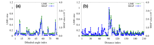
Figure S2: Dependence of feature contribution on CV index, represented in absolute values, obtained through LIME (green) and SHAP (blue) for the neural network predictions using (ii) dihedral angles + interatomic distances. Panels (a) and (b) display the index dependence of 90 dihedral angles and 210 diatomic distances, respectively.

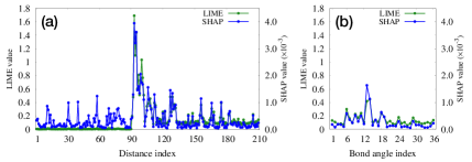
Figure S3: Dependence of feature contribution on CV index, represented in absolute values, obtained through LIME (green) and SHAP (blue) for the neural network predictions using (iii) interatomic distances + bond angles. Panels (a) and (b) display the index dependence of 210 diatomic distances and 36 bond angles, respectively.

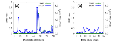
Figure S4: Dependence of feature contribution on CV index, represented in absolute values, obtained through LIME (green) and SHAP (blue) for the neural network predictions using (iv) dihedral angles + bond angles. Panels (a) and (b) display the index dependence of 90 dihedral angles and 36 bond angles, respectively.

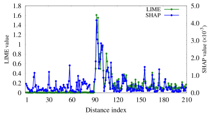
Figure S5: Dependence of feature contribution on CV index, represented in absolute values, obtained through LIME (green) and SHAP (blue) for the neural network predictions using (v) 210 interatomic distances.

References

- Zuckerman [2010] D. M. Zuckerman, Statistical Physics of Biomolecules: An Introduction (CRC press, Boca Raton, FL, 2010).
- Peters [2017] B. Peters, Reaction Rate Theory and Rare Events (Elsevier, Amsterdam, 2017).
- Ramachandran and Sasisekharan [1968] G. N. Ramachandran and V. Sasisekharan, “Conformation of Polypeptides and Proteins,” in Advances in Protein Chemistry, Vol. 23, edited by C. B. Anfinsen, M. L. Anson, J. T. Edsall, and F. M. Richards (1968) pp. 283–437.
- Bolhuis, Dellago, and Chandler [2000] P. G. Bolhuis, C. Dellago, and D. Chandler, “Reaction coordinates of biomolecular isomerization,” Proc. Natl. Acad. Sci. U.S.A. 97, 5877–5882 (2000).
- Du et al. [1998] R. Du, V. S. Pande, A. Y. Grosberg, T. Tanaka, and E. S. Shakhnovich, “On the transition coordinate for protein folding,” J. Chem. Phys. 108, 334–350 (1998).
- Geissler, Dellago, and Chandler [1999] P. L. Geissler, C. Dellago, and D. Chandler, “Kinetic Pathways of Ion Pair Dissociation in Water,” J. Phys. Chem. B 103, 3706–3710 (1999).
- Bolhuis et al. [2002] P. G. Bolhuis, D. Chandler, C. Dellago, and P. L. Geissler, “Transition Path Sampling: Throwing Ropes Over Rough Mountain Passes, in the Dark,” Annu. Rev. Phys. Chem. 53, 291–318 (2002).
- Hummer [2004] G. Hummer, “From transition paths to transition states and rate coefficients,” J. Chem. Phys. 120, 516–523 (2004).
- Best and Hummer [2005] R. B. Best and G. Hummer, “Reaction coordinates and rates from transition paths,” Proc. Natl. Acad. Sci. U.S.A. 102, 6732–6737 (2005).
- E, Ren, and Vanden-Eijnden [2005] W. E, W. Ren, and E. Vanden-Eijnden, “Transition pathways in complex systems: Reaction coordinates, isocommittor surfaces, and transition tubes,” Chem. Phys. Lett. 413, 242–247 (2005).
- Peters [2006] B. Peters, “Using the histogram test to quantify reaction coordinate error,” J. Chem. Phys. 125, 241101 (2006).
- Peters and Trout [2006] B. Peters and B. L. Trout, “Obtaining reaction coordinates by likelihood maximization,” J. Chem. Phys. 125, 054108 (2006).
- Peters, Beckham, and Trout [2007] B. Peters, G. T. Beckham, and B. L. Trout, “Extensions to the likelihood maximization approach for finding reaction coordinates,” J. Chem. Phys. 127, 034109 (2007).
- Peters [2010] B. Peters, “P(TP|) peak maximization: Necessary but not sufficient for reaction coordinate accuracy,” Chem. Phys. Lett. 494, 100–103 (2010).
- Peters [2016] B. Peters, “Reaction Coordinates and Mechanistic Hypothesis Tests,” Annu. Rev. Phys. Chem. 67, 669–690 (2016).
- Jung, Okazaki, and Hummer [2017] H. Jung, K.-i. Okazaki, and G. Hummer, “Transition path sampling of rare events by shooting from the top,” J. Chem. Phys. 147, 152716 (2017).
- Hagan et al. [2003] M. F. Hagan, A. R. Dinner, D. Chandler, and A. K. Chakraborty, “Atomistic understanding of kinetic pathways for single base-pair binding and unbinding in DNA,” Proc. Natl. Acad. Sci. U.S.A. 100, 13922–13927 (2003).
- Pan and Chandler [2004] A. C. Pan and D. Chandler, “Dynamics of Nucleation in the Ising Model,” J. Phys. Chem. B 108, 19681–19686 (2004).
- Rhee and Pande [2005] Y. M. Rhee and V. S. Pande, “One-Dimensional Reaction Coordinate and the Corresponding Potential of Mean Force from Commitment Probability Distribution,” J. Phys. Chem. B 109, 6780–6786 (2005).
- Berezhkovskii and Szabo [2005] A. Berezhkovskii and A. Szabo, “One-dimensional reaction coordinates for diffusive activated rate processes in many dimensions,” J. Chem. Phys. 122, 014503 (2005).
- Moroni, ten Wolde, and Bolhuis [2005] D. Moroni, P. R. ten Wolde, and P. G. Bolhuis, “Interplay between Structure and Size in a Critical Crystal Nucleus,” Phys. Rev. Lett. 94, 235703 (2005).
- Branduardi, Gervasio, and Parrinello [2007] D. Branduardi, F. L. Gervasio, and M. Parrinello, “From to in free energy space,” J. Chem. Phys. 126, 054103 (2007).
- Quaytman and Schwartz [2007] S. L. Quaytman and S. D. Schwartz, “Reaction coordinate of an enzymatic reaction revealed by transition path sampling,” Proc. Natl. Acad. Sci. U.S.A. 104, 12253–12258 (2007).
- Beckham et al. [2007] G. T. Beckham, B. Peters, C. Starbuck, N. Variankaval, and B. L. Trout, “Surface-Mediated Nucleation in the Solid-State Polymorph Transformation of Terephthalic Acid,” J. Am. Chem. Soc. 129, 4714–4723 (2007).
- Peters et al. [2008] B. Peters, N. E. R. Zimmermann, G. T. Beckham, J. W. Tester, and B. L. Trout, “Path Sampling Calculation of Methane Diffusivity in Natural Gas Hydrates from a Water-Vacancy Assisted Mechanism,” J. Am. Chem. Soc. 130, 17342–17350 (2008).
- Beckham, Peters, and Trout [2008] G. T. Beckham, B. Peters, and B. L. Trout, “Evidence for a Size Dependent Nucleation Mechanism in Solid State Polymorph Transformations,” J. Phys. Chem. B 112, 7460–7466 (2008).
- Antoniou and Schwartz [2009] D. Antoniou and S. D. Schwartz, “The stochastic separatrix and the reaction coordinate for complex systems,” J. Chem. Phys. 130, 151103 (2009).
- Xi, Shah, and Trout [2013] L. Xi, M. Shah, and B. L. Trout, “Hopping of Water in a Glassy Polymer Studied via Transition Path Sampling and Likelihood Maximization,” J. Phys. Chem. B 117, 3634–3647 (2013).
- Jungblut, Singraber, and Dellago [2013] S. Jungblut, A. Singraber, and C. Dellago, “Optimising reaction coordinates for crystallisation by tuning the crystallinity definition,” Mol. Phys. 111, 3527–3533 (2013).
- Barnes et al. [2014] B. C. Barnes, B. C. Knott, G. T. Beckham, D. T. Wu, and A. K. Sum, “Reaction Coordinate of Incipient Methane Clathrate Hydrate Nucleation,” J. Phys. Chem. B 118, 13236–13243 (2014).
- Mullen, Shea, and Peters [2014] R. G. Mullen, J.-E. Shea, and B. Peters, “Transmission Coefficients, Committors, and Solvent Coordinates in Ion-Pair Dissociation,” J. Chem. Theory Comput. 10, 659–667 (2014).
- Mullen, Shea, and Peters [2015] R. G. Mullen, J.-E. Shea, and B. Peters, “Easy Transition Path Sampling Methods: Flexible-Length Aimless Shooting and Permutation Shooting,” J. Chem. Theory Comput. 11, 2421–2428 (2015).
- Lupi, Peters, and Molinero [2016] L. Lupi, B. Peters, and V. Molinero, “Pre-ordering of interfacial water in the pathway of heterogeneous ice nucleation does not lead to a two-step crystallization mechanism,” J. Chem. Phys. 145, 211910 (2016).
- Ernst, Wolf, and Stock [2017] M. Ernst, S. Wolf, and G. Stock, “Identification and Validation of Reaction Coordinates Describing Protein Functional Motion: Hierarchical Dynamics of T4 Lysozyme,” J. Chem. Theory Comput. 13, 5076–5088 (2017).
- Díaz Leines and Rogal [2018] G. Díaz Leines and J. Rogal, “Maximum Likelihood Analysis of Reaction Coordinates during Solidification in Ni,” J. Phys. Chem. B 122, 10934–10942 (2018).
- Joswiak, Doherty, and Peters [2018] M. N. Joswiak, M. F. Doherty, and B. Peters, “Ion dissolution mechanism and kinetics at kink sites on NaCl surfaces,” Proc. Natl. Acad. Sci. U.S.A. 115, 656–661 (2018).
- Okazaki et al. [2019] K.-i. Okazaki, D. Wöhlert, J. Warnau, H. Jung, Ö. Yildiz, W. Kühlbrandt, and G. Hummer, “Mechanism of the electroneutral sodium/proton antiporter PaNhaP from transition-path shooting,” Nat. Commun. 10, 1742 (2019).
- Mori and Saito [2020] T. Mori and S. Saito, “Dissecting the Dynamics during Enzyme Catalysis: A Case Study of Pin1 Peptidyl-Prolyl Isomerase,” J. Chem. Theory Comput. 16, 3396–3407 (2020).
- Schwierz [2020] N. Schwierz, “Kinetic pathways of water exchange in the first hydration shell of magnesium,” J. Chem. Phys. 152, 224106 (2020).
- Silveira et al. [2021] R. L. Silveira, B. C. Knott, C. S. Pereira, M. F. Crowley, M. S. Skaf, and G. T. Beckham, “Transition Path Sampling Study of the Feruloyl Esterase Mechanism,” J. Phys. Chem. B 125, 2018–2030 (2021).
- Sittel and Stock [2016] F. Sittel and G. Stock, “Robust Density-Based Clustering To Identify Metastable Conformational States of Proteins,” J. Chem. Theory Comput. 12, 2426–2435 (2016).
- Sultan and Pande [2018] M. M. Sultan and V. S. Pande, “Automated design of collective variables using supervised machine learning,” J. Chem. Phys. 149, 094106 (2018).
- Wehmeyer and Noé [2018] C. Wehmeyer and F. Noé, “Time-lagged autoencoders: Deep learning of slow collective variables for molecular kinetics,” J. Chem. Phys. 148, 241703 (2018).
- Mardt et al. [2018] A. Mardt, L. Pasquali, H. Wu, and F. Noé, “VAMPnets for deep learning of molecular kinetics,” Nat. Commun. 9, 5 (2018).
- Bittracher, Banisch, and Schütte [2018] A. Bittracher, R. Banisch, and C. Schütte, “Data-driven computation of molecular reaction coordinates,” J. Chem. Phys. 149, 154103 (2018).
- Chen and Ferguson [2018] W. Chen and A. L. Ferguson, “Molecular enhanced sampling with autoencoders: On-the-fly collective variable discovery and accelerated free energy landscape exploration,” J. Comput. Chem. 39, 2079–2102 (2018).
- Ribeiro et al. [2018] J. M. L. Ribeiro, P. Bravo, Y. Wang, and P. Tiwary, “Reweighted autoencoded variational Bayes for enhanced sampling (RAVE),” J. Chem. Phys. 149, 072301 (2018).
- Rogal, Schneider, and Tuckerman [2019] J. Rogal, E. Schneider, and M. E. Tuckerman, “Neural-Network-Based Path Collective Variables for Enhanced Sampling of Phase Transformations,” Phys. Rev. Lett. 123, 245701 (2019).
- Wang, Lamim Ribeiro, and Tiwary [2020] Y. Wang, J. M. Lamim Ribeiro, and P. Tiwary, “Machine learning approaches for analyzing and enhancing molecular dynamics simulations,” Curr. Opin. Struct. Biol. 61, 139–145 (2020).
- Bonati, Rizzi, and Parrinello [2020] L. Bonati, V. Rizzi, and M. Parrinello, “Data-Driven Collective Variables for Enhanced Sampling,” J. Phys. Chem. Lett. 11, 2998–3004 (2020).
- Sidky, Chen, and Ferguson [2020] H. Sidky, W. Chen, and A. L. Ferguson, “Machine learning for collective variable discovery and enhanced sampling in biomolecular simulation,” Mol. Phys. 118, e1737742 (2020).
- Wang and Tiwary [2021] D. Wang and P. Tiwary, “State predictive information bottleneck,” J. Chem. Phys. 154, 134111 (2021).
- Zhang et al. [2021] J. Zhang, Y.-K. Lei, Z. Zhang, X. Han, M. Li, L. Yang, Y. I. Yang, and Y. Q. Gao, “Deep reinforcement learning of transition states,” Phys. Chem. Chem. Phys. 23, 6888–6895 (2021).
- Frassek, Arjun, and Bolhuis [2021] M. Frassek, A. Arjun, and P. G. Bolhuis, “An extended autoencoder model for reaction coordinate discovery in rare event molecular dynamics datasets,” J. Chem. Phys. 155, 064103 (2021).
- Hooft, Pérez de Alba Ortíz, and Ensing [2021] F. Hooft, A. Pérez de Alba Ortíz, and B. Ensing, “Discovering Collective Variables of Molecular Transitions via Genetic Algorithms and Neural Networks,” J. Chem. Theory Comput. 17, 2294–2306 (2021).
- Bonati, Piccini, and Parrinello [2021] L. Bonati, G. Piccini, and M. Parrinello, “Deep learning the slow modes for rare events sampling,” Proc. Natl. Acad. Sci. U.S.A. 118, e2113533118 (2021).
- Chen [2021] M. Chen, “Collective variable-based enhanced sampling and machine learning,” Eur. Phys. J. B 94, 211 (2021).
- Belkacemi et al. [2021] Z. Belkacemi, P. Gkeka, T. Lelièvre, and G. Stoltz, “Chasing Collective Variables Using Autoencoders and Biased Trajectories,” J. Chem. Theory Comput. , acs.jctc.1c00415 (2021).
- Neumann and Schwierz [2022] J. Neumann and N. Schwierz, “Artificial Intelligence Resolves Kinetic Pathways of Magnesium Binding to RNA,” J. Chem. Theory Comput. 18, 1202–1212 (2022).
- Ray, Trizio, and Parrinello [2023] D. Ray, E. Trizio, and M. Parrinello, “Deep learning collective variables from transition path ensemble,” J. Chem. Phys. 158, 204102 (2023).
- Jung et al. [2023] H. Jung, R. Covino, A. Arjun, C. Leitold, C. Dellago, P. G. Bolhuis, and G. Hummer, “Machine-guided path sampling to discover mechanisms of molecular self-organization,” Nat. Comput. Sci. 3, 334–345 (2023).
- Bonati et al. [2023] L. Bonati, E. Trizio, A. Rizzi, and M. Parrinello, “A unified framework for machine learning collective variables for enhanced sampling simulations: Mlcolvar,” J. Chem. Phys. 159, 014801 (2023).
- Singh and Limmer [2023] A. N. Singh and D. T. Limmer, “Variational deep learning of equilibrium transition path ensembles,” J. Chem. Phys. 159, 024124 (2023).
- Liang et al. [2023] S. Liang, A. N. Singh, Y. Zhu, D. T. Limmer, and C. Yang, “Probing reaction channels via reinforcement learning,” Mach. Learn.: Sci. Technol. 4, 045003 (2023).
- Lazzeri et al. [2023] G. Lazzeri, H. Jung, P. G. Bolhuis, and R. Covino, “Molecular Free Energies, Rates, and Mechanisms from Data-Efficient Path Sampling Simulations,” J. Chem. Theory Comput. , acs.jctc.3c00821 (2023).
- Ma and Dinner [2005] A. Ma and A. R. Dinner, “Automatic Method for Identifying Reaction Coordinates in Complex Systems,” J. Phys. Chem. B 109, 6769–6779 (2005).
- Mori et al. [2020] Y. Mori, K.-i. Okazaki, T. Mori, K. Kim, and N. Matubayasi, “Learning reaction coordinates via cross-entropy minimization: Application to alanine dipeptide,” J. Chem. Phys. 153, 054115 (2020).
- Kikutsuji et al. [2022] T. Kikutsuji, Y. Mori, K.-i. Okazaki, T. Mori, K. Kim, and N. Matubayasi, “Explaining reaction coordinates of alanine dipeptide isomerization obtained from deep neural networks using Explainable Artificial Intelligence (XAI),” J. Chem. Phys. 156, 154108 (2022).
- Manuchehrfar et al. [2021] F. Manuchehrfar, H. Li, W. Tian, A. Ma, and J. Liang, “Exact Topology of the Dynamic Probability Surface of an Activated Process by Persistent Homology,” J. Phys. Chem. B 125, 4667–4680 (2021).
- Naleem et al. [2023] N. Naleem, C. R. A. Abreu, K. Warmuz, M. Tong, S. Kirmizialtin, and M. E. Tuckerman, “An exploration of machine learning models for the determination of reaction coordinates associated with conformational transitions,” J. Chem. Phys. 159, 034102 (2023).
- Ribeiro, Singh, and Guestrin [2016] M. T. Ribeiro, S. Singh, and C. Guestrin, “”Why Should I Trust You?”: Explaining the Predictions of Any Classifier,” in Proceedings of the 22nd ACM SIGKDD International Conference on Knowledge Discovery and Data Mining (San Francisco California, U.S.A., 2016) pp. 1135–1144.
- Lundberg and Lee [2017] S. M. Lundberg and S.-I. Lee, “A unified approach to interpreting model predictions,” in Proceedings of the 31st international conference on neural information processing systems (2017) pp. 4768–4777.