Frequency-aware Graph Signal Processing for Collaborative Filtering

Abstract.

Graph Signal Processing (GSP) based recommendation algorithms have recently attracted lots of attention due to its high efficiency. However, these methods failed to consider the importance of various interactions that reflect unique user/item characteristics and failed to utilize user and item high-order neighborhood information to model user preference, thus leading to sub-optimal performance. To address the above issues, we propose a frequency-aware graph signal processing method (FaGSP) for collaborative filtering. Firstly, we design a Cascaded Filter Module, consisting of an ideal high-pass filter and an ideal low-pass filter that work in a successive manner, to capture both unique and common user/item characteristics to more accurately model user preference. Then, we devise a Parallel Filter Module, consisting of two low-pass filters that can easily capture the hierarchy of neighborhood, to fully utilize high-order neighborhood information of users/items for more accurate user preference modeling. Finally, we combine these two modules via a linear model to further improve recommendation accuracy. Extensive experiments on six public datasets demonstrate the superiority of our method from the perspectives of prediction accuracy and training efficiency compared with state-of-the-art GCN-based recommendation methods and GSP-based recommendation methods.

1. Introduction

Graph Signal Processing (GSP) (Ortega et al., 2018; Dong et al., 2020; Stanković et al., 2019) extends signal processing techniques to graph data, which first transforms signals into frequency domain and then processes specific frequency components to extract and analyze information existed in the signal based on spectral graph theory (Chung, 1997; Spielman, 2007). Currently, GSP-based recommendation algorithms (Shen et al., 2021; Liu et al., 2023; Huang et al., 2017) are receiving increasing attention from researchers due to its parameter-free characteristic. Compared with graph-based collaborative filtering methods, these non-parametric methods do not suffer from a time-consuming training phase and thus are highly efficient, while can achieve comparable or better performance than deep learning-based methods (He et al., 2020; Mao et al., 2021a; Wu et al., 2021a; Song et al., 2010; Sun et al., 2020).

Generally, user interactions contain rich information that depicts user interests and item characteristics. Through designing and exerting different types of filters on user interactions, we can extract different types of information to model user preference, thereby improving the accuracy of user future interaction prediction. GF-CF (Shen et al., 2021) and PGSP (Liu et al., 2023) are two representative GSP-based collaborative filtering methods, both of which adopt an ideal low-pass filter and a linear filter to extract information from user/item common characteristic and user and item first-order neighborhood respectively. Though they have shown promising performance, two limitations restrict their expressivity in modeling user preference.

The first limitation is that they focus on user/item common characteristics and neglect their unique characteristics. Common characteristics refer to the shared features among many users/items, such as a broad target audience aged 18-60, while the unique characteristics refer to those characteristics that can distinguish a user/item from others, such as a narrow target audience aged 18-25, both of which are implicit in user interactions. When they use the ideal low-pass filters to predict user future interactions, merely common characteristics will be utilized for prediction, while unique characteristics will be filtered out. Obviously, in this way, they can only roughly recommend items to users based on common characteristics, making the predictions sub-optimal. The second limitation is that they fail to fully utilize user and item high-order neighborhood information. The powerful modeling capacity of GCN (Kipf and Welling, 2017; Xu et al., [n. d.]) mainly benefits from aggregating information from both direct and distant neighbors. By analogy, we can infer that user and item high-order neighborhood information, which is obtained by aggregating information from their neighbors of different distances, can also be crucial to model user preference, so as to extract richer information for interaction prediction. However, linear filters, designed on the user/item co-occurrence relationship, can only extract information from first-order neighborhood, leading to insufficient modeling of user preference and sub-optimal performance.

In this work, we propose a frequency-aware graph signal processing method (FaGSP) for collaborative filtering to address the above two limitations. Firstly, we design a Cascaded Filter Module to take both common characteristics and unique characteristics into consideration for interaction prediction, which first uses an ideal high-pass filter to enhance interaction signal by highlighting those interactions that reflect unique characteristics, then uses an ideal low-pass filter over the enhanced signal to predict future interactions. Secondly, we devise a Parallel Filter Module consisting of two low-pass filters, which are designed to capture user and item high-order neighborhood information respectively for user preference modeling. By adjusting the parameters of these two filters, they are capable of capturing information from neighborhood with any order. Finally, we combine these two modules via a linear model to make FaGSP able to extract rich information from user interactions for user preference modeling and interaction prediction. We conduct extensive experiments on six real-world datasets, and the experimental results demonstrate the superiority of our method from the perspectives of recommendation accuracy and training efficiency compared with existing GCN/GSP-based collaborative filtering methods.

2. Preliminaries

2.1. Graph Signal Processing

2.1.1. Graph Signal

Given an undirected and unweighted graph $\mathcal{G}=(\mathcal{N},\mathcal{E})$, where $\mathcal{N}$ and $\mathcal{E}$ represent the node set and edge set respectively, and $|\mathcal{N}|=n$. The graph structure can be represented as an adjacency matrix $\mathbf{A}\in\mathbb{R}^{n\times n}$, and if there is an edge between node $i$ and node $j$, $\mathbf{A}_{ij}=1$, otherwise, $\mathbf{A}_{ij}=0$. The graph laplacian matrix, defined over $\mathcal{G}$, can be represented as $\mathbf{L}=\mathbf{D}-\mathbf{A}$, where $\mathbf{D}=diag(\mathbf{A}\cdot\mathbf{1})\in\mathbb{R}^{n\times n}$ is the degree matrix, and the corresponding normalized laplacian matrix is $\tilde{\mathbf{L}}=\mathbf{D}^{-\frac{1}{2}}\mathbf{L}\mathbf{D}^{-\frac{1}{2}}$. As the normalized graph laplacian matrix is a real and symmetric matrix, it can be decomposed into ${\tilde{\mathbf{L}}}=\mathbf{U}\boldsymbol{\Lambda}\mathbf{U}^{T}$, where $\boldsymbol{\Lambda}=diag(\lambda_{1},\lambda_{2},\cdots,\lambda_{n})$ and $\mathbf{U}=(\mathbf{u}_{1},\mathbf{u}_{2},\cdots,\mathbf{u}_{n})$ are the eigenvalue matrix and eigenvector matrix respectively, and $0\leq\lambda_{1}\leq\lambda_{2}\leq\cdots\leq\lambda_{n}\leq 2$. The graph signal can be defined by a mapping $h:\mathcal{N}\rightarrow\mathbb{R}$, and it can be represented as a vector $\mathbf{x}=\{x_{1},x_{2},\cdots,x_{n}\}$, where $x_{i}$ is the signal strength of the $i$-th node. The graph quadratic form is widely used to measure the smoothness of the graph signal, which is defined as

(1) $$S(\mathbf{x})=\frac{\mathbf{x}^{T}{\mathbf{L}}\mathbf{x}}{||\mathbf{x}||_{2}}.$$

If $S(\mathbf{x_{1}})<S(\mathbf{x_{2}})$, then the graph signal $\mathbf{x}_{1}$ is smoother than $\mathbf{x}_{2}$.

2.1.2. Graph Filter

GSP uses graph filter $\mathcal{F}$ to analyse graph signal:

(2) $$\mathcal{F}=\mathbf{U}diag(f(\lambda_{1}),f(\lambda_{2}),\cdots,f(\lambda_{n}))\mathbf{U}^{T}=\mathbf{U}\mathbf{F}\mathbf{U}^{T},$$

where $\mathbf{U}$ is the eigenvector matrix of normalized laplacian matrix $\tilde{\mathbf{L}}$. $f(\cdot)$ is a frequency response function that determines whether some frequency component $\lambda_{i}$ is enhanced or attenuated. Different design of $f(\cdot)$ will lead to the different graph filter $\mathcal{F}$, if $f(\cdot)$ is a monotonic decreasing function, then $\mathcal{F}$ is a low-pass filter, and if $f(\cdot)$ is a monotonic increasing function, then $\mathcal{F}$ is a high-pass filter. Low-pass filter and high-pass filter have different effects to the graph signal $\mathbf{x}$, as shown in the Proposition 2.1.

Proposition 0.

Low-pass filter can smooth the graph signal $\mathbf{x}$, i.e., reduce $S(\mathbf{x})$, while high-pass filter can coarsen the graph signal $\mathbf{x}$, i.e., enhance $S(\mathbf{x})$.

Proof.

Since ${\mathbf{L}}$ is a real and symmetric matrix, it is diagonalizable ${\mathbf{L}}=\mathbf{U}\boldsymbol{\Lambda}\mathbf{U}^{T}$, thus $S(\mathbf{x})$ can be represented as:

(3) $$S_{1}(\mathbf{x}) =\frac{\mathbf{x}^{T}{\mathbf{L}}\mathbf{x}}{\mathbf{x}^{T}\mathbf{x}}=\frac{\mathbf{x}^{T}\mathbf{U}\mathbf{\Lambda}\mathbf{U}^{T}\mathbf{x}}{\mathbf{x}^{T}\mathbf{U}\mathbf{U}^{T}\mathbf{x}}=\frac{\mathbf{y}^{T}\mathbf{\Lambda}\mathbf{y}}{\mathbf{y}^{T}\mathbf{y}}=\frac{\sum_{i=1}^{n}\lambda_{i}y_{i}^{2}}{\sum_{i=1}^{n}y_{i}^{2}},$$

where $\mathbf{U}$ is the orthogonal eigenvector matrix ($\mathbf{U}^{T}\mathbf{U}=\mathbf{U}\mathbf{U^{T}}=\mathbf{I}$), and we denote $\mathbf{y}={\mathbf{U}}^{T}\mathbf{x}$, and $y_{i}=\mathbf{u}_{i}^{T}\mathbf{x}$. Suppose there is a filter $\mathcal{F}=\mathbf{U}\mathbf{F}\mathbf{U}^{T}$ exerting on the signal $\mathbf{x}$ and inducing a new graph signal $\mathbf{z}=\mathcal{F}\mathbf{x}$. The corresponding smoothness of graph signal $\mathbf{z}$ is

(4) $$S_{2}(\mathbf{z}) =\frac{\mathbf{z}^{T}{\mathbf{L}}\mathbf{z}}{\mathbf{z}^{T}\mathbf{z}}=\frac{\mathbf{x}^{T}\mathbf{U}\mathbf{F}\mathbf{\Lambda}\mathbf{F}\mathbf{U}^{T}\mathbf{x}}{\mathbf{x}^{T}\mathbf{U}\mathbf{F}^{2}\mathbf{U}^{T}\mathbf{x}}=\frac{\sum_{i=1}^{n}f_{i}^{2}\lambda_{i}y_{i}^{2}}{\sum_{i=1}^{n}f_{i}^{2}y_{i}^{2}},$$

where $f_{i}=f(\lambda_{i})$. Thus, the change of smoothness is

(5) $$\Delta S =S_{2}(\mathbf{z})-S_{1}(\mathbf{x})=\frac{\sum_{i=1}^{n}\sum_{j>i}^{n}(f_{i}^{2}-f_{j}^{2})(\lambda_{i}-\lambda_{j})y_{i}^{2}y_{j}^{2}}{\left(\sum_{i=1}^{n}f_{i}^{2}y_{i}^{2}\right)\left(\sum_{i=1}^{n}y_{i}^{2}\right)}.$$

When $\mathcal{F}$ is a low-pass filter with $f_{i}>f_{j}$ for $\lambda_{i}<\lambda_{j}$, then

(6) $$\Delta S =\frac{\sum_{i=1}^{n}\sum_{j>i}^{n}(f_{i}^{2}-f_{j}^{2})(\lambda_{i}-\lambda_{j})y_{i}^{2}y_{j}^{2}}{\left(\sum_{i=1}^{m}f_{i}^{2}y_{i}^{2}\right)\left(\sum_{i=1}^{n}y_{i}^{2}\right)}<0,$$

$\Delta S$¡0 means the graph signal becomes smoother. Therefore, low-pass filter can smooth the graph signal. When $\mathcal{F}$ is a high-pass filter with $f_{i}<f_{j}$ for $\lambda_{i}<\lambda_{j}$, then

(7) $$\Delta S =\frac{\sum_{i=1}^{n}\sum_{j>i}^{n}(f_{i}^{2}-f_{j}^{2})(\lambda_{i}-\lambda_{j})y_{i}^{2}y_{j}^{2}}{\left(\sum_{i=1}^{m}f_{i}^{2}y_{i}^{2}\right)\left(\sum_{i=1}^{n}y_{i}^{2}\right)}>0.$$

$\Delta S$¿0 means the graph signal becomes coarser. Therefore, high-pass filter can coarsen the graph signal. ∎

2.1.3. Graph Convolution

Instead of spatial domain, GSP processes graph signal in spectral domain. Therefore, the graph signal processing of a given graph signal $\mathbf{x}$ can be regarded as the graph convolution over the signal $\mathbf{x}$:

(8) $$\mathbf{y}=\mathcal{F}\mathbf{x}=\mathbf{U}diag(f(\lambda_{1}),f(\lambda_{2}),\cdots,f(\lambda_{n}))\mathbf{U}^{T}\mathbf{x}.$$

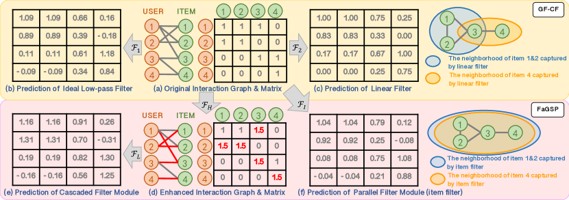
Figure 1. A toy example of user interaction prediction with 4 users and 4 items. (a) is the original interaction matrix, (b) and (c) are the prediction of the ideal low-pass filter and linear filter in GF-CF respectively. (d) is the enhanced interaction matrix, (e)–(f) are the predictions of the Cascaded Filter Module and Parallel Filter Module in FaGSP respectively. For ideal high-pass filter to enhance interactions in (d), we set $p_{1}=2$, $q=0.65$, and $\alpha_{1}=0.5$. For ideal low-pass filter in (b) and (d), we set $p_{2}=2$. In Parallel Filter Module, we only consider item high-order neighborhood information for the ease of presentation.

The signal $\mathbf{x}$ is first transformed from spatial domain to the spectral domain through Graph Fourier Transform basis $\mathbf{U}^{T}$, then the undesired frequencies are removed in the signal through function $f(\cdot)$ in spectral domain, and finally signal is transformed back to spatial domain through inverse Graph Fourier Transform basis $\mathbf{U}$.

2.2. Notations

Let the user set and item set be $\mathcal{U}$ and $\mathcal{V}$, and $|\mathcal{U}|=m$ and $|\mathcal{V}|=n$. The interactions between users and items can be represented as an interaction matrix $\mathbf{R}\in\{0,1\}^{m\times n}$, and if there is an interaction between user $u$ and item $i$, then $\mathbf{R}_{ui}=1$, otherwise, $\mathbf{R}_{ui}=0$. The normalized interaction matrix can be defined as $\tilde{\mathbf{R}}=\mathbf{D}_{U}^{-\frac{1}{2}}\mathbf{R}\mathbf{D}_{I}^{-\frac{1}{2}}$, where $\mathbf{D}_{U}=diag(\mathbf{R}\cdot\mathbf{1})$ and $\mathbf{D}_{I}=diag(\mathbf{R}^{T}\cdot\mathbf{1})$ are the user degree matrix and item degree matrix respectively. Then we can define user/item co-occurrence relationship matrix as follows:

(9) $$\mathbf{O}_{U}=\tilde{\mathbf{R}}\tilde{\mathbf{R}}^{T},\quad\mathbf{O}_{I}=\tilde{\mathbf{R}}^{T}\tilde{\mathbf{R}}.$$

2.3. The GF-CF and PGSP methods

GF-CF (Shen et al., 2021) adopted a combined filter to model user preference

(10) $$\mathcal{F}=\alpha\mathbf{D}_{I}^{-\frac{1}{2}}\mathbf{V}_{k}\mathbf{V}_{k}^{T}\mathbf{D}_{I}^{\frac{1}{2}}+\mathbf{O}_{I},$$

where $\mathbf{V}_{k}$ is the eigenvector matrix corresponding to the $k$ largest eigenvalues of $\mathbf{O}_{I}$, but in practice, it is obtained by perform Singular Value Decomposition (SVD) (Paterek, 2007) on $\tilde{\mathbf{R}}$ for high efficiency. $\alpha$ is a hyper-parameter that balances the two terms. Formally, GF-CF is composed of two types of filters: (1) an ideal low-pass filter $\mathcal{F}_{1}=\mathbf{D}_{I}^{-\frac{1}{2}}\mathbf{V}_{k}\mathbf{V}_{k}^{T}\mathbf{D}_{I}^{\frac{1}{2}}$, and (2) a linear filter $\mathcal{F}_{2}=\mathbf{O}_{I}$. PGSP (Liu et al., 2023) designed a mixed-frequency filter to predict user future interactions

(11) $$\mathcal{F}=(1-\phi)\bar{\mathbf{V}}_{k}\bar{\mathbf{V}}_{k}^{T}+\phi\mathbf{A},$$

where $\bar{\mathbf{V}}_{k}$ is the eigenvector matrix corresponding to the first $k$ smallest eigenvalues of graph laplacian matrix $\mathbf{L}=\mathbf{I}-\mathbf{A}$, and $\mathbf{A}=\begin{bmatrix}\mathbf{O}_{U}&\tilde{\mathbf{R}}\\ \tilde{\mathbf{R}}^{T}&\mathbf{O}_{I}\end{bmatrix}$ is the augmented similarity graph. PGSP is also composed of two filters: (1) an ideal low-pass filter $\mathcal{F}_{1}=\bar{\mathbf{V}}_{k}\bar{\mathbf{V}}_{k}^{T}$ and (2) a linear filter $\mathcal{F}_{2}=\mathbf{A}$.

2.4. Motivation

In this section, we take GF-CF method (Shen et al., 2021) as an example to briefly illustrate the problems of existing GSP-based recommendation algorithms, which use an ideal low-pass filter and a linear filter to predict user future interactions, on a toy example composed of 4 users and 4 items. Figure 1 (b) and (c) show the results of user interaction prediction when using an ideal low-pass filter and a linear filter of GF-CF. We analyze the predictions as follows:

Ideal low-pass filter. When predicting the interaction scores of $u_{2}$ (user 2) to $i_{2}$ and $i_{3}$ (item 2 and item 3), the difference between two scores is roughly the same as that between the interaction scores of $u_{1}$ to $i_{2}$ and $i_{3}$. This is because there is a connection between $i_{2}$ and $i_{3}$, that is, they are both interacted with by $u_{1}$, and the ideal low-pass filter can capture item common characteristic to smooth the graph signal, reducing the differences in predictions of $i_{2}$ and $i_{3}$. However, it ignores the item unique characteristic, that is, the target audience of $i_{2}$ is $u_{1}$ and $u_{2}$, while the target audience of $i_{3}$ is $u_{1}$ and $u_{3}$. Therefore, the difference in $u_{2}$’s interaction scores to $i_{2}$ and $i_{3}$ should be greater than that in $u_{1}$’s interaction scores to $i_{2}$ and $i_{3}$, and similar conclusions can be drawn for $u_{3}$. In addition, the relationship between $i_{3}$ and $i_{4}$ makes $u_{4}$ become a potential target audience of $i_{3}$, but not necessarily a potential target audience of $i_{2}$. Therefore, when predicting whether $u_{4}$ will interact with $i_{2}$ and $i_{3}$, the latter score should be significantly higher than the former.

Linear filter. When predicting $u_{4}$’s future interactions, linear filters only focus on the interaction between $u_{4}$ and $i_{3}$, while ignoring that between $u_{4}$ and $i_{1}$(or $i_{2}$), although $i_{1}$ and $i_{2}$ also have a latent connection with the interacted $i_{4}$, for example, $i_{1}$ and $i_{4}$ have an indirect relationship through $i_{3}$. Similarly, when predicting $u_{2}$’s future interactions, the filter only focuses on $i_{3}$, while ignoring $i_{4}$. This is because linear filters are constructed on the item co-occurrence matrix $\mathbf{O}_{I}$, and essentially can merely capture direct relationships between items. When using linear filters to predict user interactions, only items that have direct correlations to the user’s interacted items can be predicted, while items that have indirect correlations cannot be predicted, resulting in limited coverage and inaccurate prediction results.

Therefore, the issues of ideal low-pass filter and linear filter motivates us to design more suitable filters to extract richer information from user interactions, so as to make user preference modeling and interaction prediction accurately.

3. The Proposed Method

In this section, we introduce FaGSP, a frequency-aware graph signal processing method for collaborative filtering, to model user preference through two carefully designed filter modules: (1) a Cascaded Filter Module used to model user preference using both unique and common characteristics, and (2) a Parallel Filter Module used to model user preference using user and item high-order neighborhood information. By combining these two modules, we can make the modeling of user preference more precise, thereby restore users’ real interactive intentions and predict their future interactions more accurately.

3.1. Cascaded Filter Module

The proposition 2.1 shows that low-pass filter can make the graph signal smoother, which is equal to retain the common characteristics among nodes and ignore the unique characteristics. Therefore, the ideal low-pass filters that existing GSP-based CF methods adopt can only capture common characteristics but fail to capture unique characteristics. Fortunately, ideal high-pass filter can capture unique characteristics since it coarsens graph signal to make nodes able to retain their own characteristics. Thus, we propose the Cascaded Filter Module, which is composed of an ideal high-pass filter and an ideal low-pass filter that work in a cascaded manner, to address the issue of the ideal low-pass filter.

First, we perform SVD on the normalized interaction matrix $\tilde{\mathbf{R}}$

(12) $$\tilde{\mathbf{R}}=\mathbf{U}\mathbf{\Lambda}\mathbf{V},$$

where singular values in $\mathbf{\Lambda}$ are arranged in descending order. We take the last $p_{1}$ rows of $\mathbf{V}$ (i,e., $\mathbf{V}_{-p_{1}:}$), which corresponds to the $p_{1}$ high frequency components, to construct the ideal high-pass filter as follows:

(13) $$\mathcal{F}_{H}=\mathbf{D}^{-\frac{1}{2}}_{I}\mathbf{V}_{-p_{1}:}\mathbf{V}_{-p_{1}:}^{T}\mathbf{D}^{\frac{1}{2}}_{I}.$$

Then, we exert $\mathcal{F}_{H}$ on the interaction signal $\mathbf{R}$ and obtain predicted matrix $\mathbf{R}^{*}$ whose element $\mathbf{R}^{*}_{u,i}$ is proportional to the probability that the corresponding interaction can reflect unique characteristics

(14) $$\mathbf{R}^{*}=\mathbf{R}\mathcal{F}_{H}.$$

In order to filter out those interactions that truly reflect unique characteristics in $\mathbf{R}^{*}$, we first calculate the $q$ quantile of $\mathbf{R}^{*}_{:,i}$ (the $i$-th column of $\mathbf{R}^{*}$) for each item $i$, which we denote as $r^{q}_{i}$. Then by comparing $\mathbf{R}^{*}_{:,i}$ and $r^{q}_{i}$, we can obtain those interactions that reflect unique characteristics, formed as $\mathbf{R}_{H}$

(15) $$(\mathbf{R}_{H})_{u,i}=\left\{\begin{matrix}1,&\text{~{}if~{}}\mathbf{R}^{*}_{u,i}\geq r^{q}_{i}~{}\text{and}~{}\mathbf{R}_{u,i}>0,\\ 0,&\text{~{}otherwise.}\end{matrix}\right.$$

Note that these interactions should also be user historical interactions, i.e., $\mathbf{R}_{u,i}>0$. Finally, we can obtain the enhanced interaction signal $\hat{\mathbf{R}}$ by highlighting those interactions in $\mathbf{R}$ with $\mathbf{R}_{H}$

(16) $$\hat{\mathbf{R}}=\mathbf{R}+\alpha_{1}\cdot\mathbf{R}_{H},$$

where $\alpha_{1}\in\mathbb{R}^{+}$ is to control the impacts of common characteristics and unique characteristics on user preference modeling and future interaction prediction. Smaller $\alpha_{1}$ will make the model focus on common characteristics, while larger $\alpha_{1}$ will emphasize the importance of unique characteristics.

After obtaining the enhanced interaction signal $\hat{\mathbf{R}}$, we perform SVD on it to construct an ideal low-pass filter as follows:

(17) $$\mathcal{F}_{L}=\hat{{\mathbf{D}}}^{-\frac{1}{2}}_{I}\hat{\mathbf{V}}_{:p_{2}}{\hat{\mathbf{V}}}_{:p_{2}}^{T}\hat{{\mathbf{D}}}^{\frac{1}{2}}_{I},$$

where $\hat{\mathbf{V}}_{:p_{2}}$ is constructed by the first $p_{2}$ rows of singular vector matrix $\hat{\mathbf{V}}$ of $\hat{\mathbf{R}}$, and $\hat{\mathbf{D}}_{I}=diag(\hat{\mathbf{R}}^{T}\cdot\mathbf{1})$. Then we use the filter to predict user future interactions as follows:

(18) $$\mathbf{P}_{1}=\hat{\mathbf{R}}\mathcal{F}_{L}.$$

It is worth noting that the ideal low-pass filter is designed on the enhanced interaction signal instead of the original interaction signal, thus the unique characteristics are taken into consideration when predicting user future interaction. Compared to merely using ideal low-pass filter ($\alpha_{1}=0$), Cascaded Filter Module can fully utilize unique characteristics and common characteristics from user interactions to jointly model user preference by exerting ideal high-pass filter and ideal low-pass filter in a cascaded manner, leading to more accurate interaction prediction.

The interactions marked in red in Figure 1 (d)—which are recognized by ideal high-pass filter—are those interactions that reflect unique characteristics. The results are reasonable, for example, the unique characteristic of $i_{4}$ should be reflected by its interaction with $u_{4}$ because there are no other users except $u_{4}$ interacting with $i_{4}$, which indicates the unique characteristics of $i_{4}$, e.g., the target audience such as $u_{4}$. Similarly, the interactions between $u_{3}$ and $i_{3}$ can reflect the unique characteristic of $i_{3}$. The Figure 1 (e) shows the interaction prediction of Cascaded Filter Module in FaGSP. Comparing to Figure 1 (b), we can find that the difference in predicted scores of $u_{4}$ to $i_{2}$ and $i_{3}$ increases, and the score of the latter is significantly higher than that of the former, which aligns with our analysis in Section 2.4, that is, $i_{3}$ has a higher degree of matching with $u_{4}$’s preference compared to $i_{2}$.

3.2. Parallel Filter Module

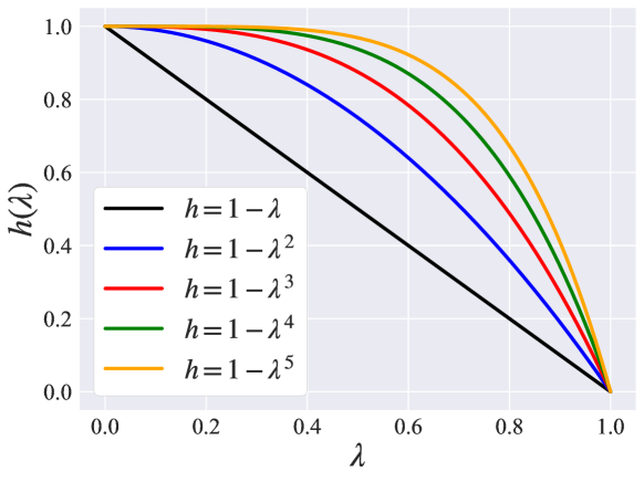
Figure 2. The frequency response functions $h(\lambda)=1-\lambda^{k_{1}}$ with respect to different order $k_{1}$ ranging from 1 to 5.

To address the issue that existing GSP-based CF methods cannot capture user and item high-order neighborhood information, we propose the Parallel Filter Module to capture user and item high-order neighborhood characteristics respectively. Since the process of extracting user and item higher-order neighborhood information is the same, we take item as an example to illustrate how to extract this characteristic. We design the item low-pass filter as follows:

(19) $$\mathcal{F}_{I}=\mathbf{I}-(\mathbf{I}-\mathbf{O}_{I})^{k_{1}},$$

where $\mathbf{O}_{I}=\tilde{\mathbf{R}}^{T}\tilde{\mathbf{R}}$, and $k_{1}(k_{1}\geq 2)$ is the order of the low-pass filter and controls the range of neighborhood information extraction. The design of the filter is based on the following two considerations: one is that it can capture neighborhood information with any order. As $k_{1}$ increases, more distant neighborhood information can be extracted. Note that when $k_{1}=1$, $\mathcal{F}_{I}$ degenerates to a linear filter $\mathcal{F}=\mathbf{O}_{I}$ that existing GSP-based CF methods adopt.

Proposition 3.1 shows that the frequency response function of $\mathcal{F}_{I}$ is a non-linear concave function, which reveals the other consideration for the design of the filter, i.e., preserving the common and unique characteristics in the high-order neighborhood of item.

Proposition 0.

The frequency response function of $\mathcal{F}_{I}$ is a non-linear concave function.

Proof.

Let $\mathbf{L}_{I}=\mathbf{I}-\mathbf{O}_{I}$. Since both $\mathbf{I}$ and $\mathbf{O}_{I}$ are real and symmetric matrices, $\mathbf{L}_{I}$ is also a real and symmetric matrix, thus $\mathbf{L}_{I}$ is diagonalizable and can be represented as $\mathbf{L}_{I}=\mathbf{U}\boldsymbol{\Lambda}\mathbf{U}^{T}$, and $\mathbf{U}\mathbf{U}^{T}=\mathbf{U}^{T}\mathbf{U}=\mathbf{I}$. Then we have

(20) $$\mathcal{F}_{I} =\mathbf{I}-(\mathbf{I}-\mathbf{O}_{I})^{k_{1}}=\mathbf{U}\mathbf{U}^{T}-\mathbf{U}\boldsymbol{\Lambda}^{k_{1}}\mathbf{U}^{T}=\mathbf{U}(\mathbf{I}-\boldsymbol{\Lambda}^{k_{1}})\mathbf{U}^{T}.$$

By comparing Eq. (2) and Eq. (20), we can easily find that the frequency response function of $\mathcal{F}_{I}$ is $f(\lambda_{i})=1-\lambda_{i}^{k_{1}}$, where $\lambda_{i}$ is the $i$-th eigenvalue of $\mathbf{L}_{I}$, and its range is [0,1], which is proved in GF-CF (Shen et al., 2021). When $k_{1}\geq 2$, it is obviously a non-linear concave function, since for any $\lambda_{i},\lambda_{j}\in[0,1]$ and $\beta\in[0,1]$, we have $f\left((1-\beta)\times\lambda_{i}+\beta\times\lambda_{j}\right)\geq(1-\beta)\times f(\lambda_{i})+\beta\times f(\lambda_{j})$ . ∎

Figure 2 shows the frequency response functions with respect to different order of filter $k_{1}$ ranging from 1 to 5. We can find that when $k_{1}=1$, the frequency response function of linear filter (black curve) is linear, both low frequency and high frequency are attenuated, making it unable to capture common and unique characteristics in direct neighborhood of item for interaction prediction. However, when $k_{1}$ grows, the frequency response function (colored curves) becomes non-linear, and more and more low frequency components are preserved and high frequency components are enhanced. For example, when $k_{1}=2$, around 3.2% low frequency components can be retained since $h(0.032)=1-0.032^{2}=0.999\approx 1$, while when $k_{1}=5$, around 25.1% low frequency components can be retained. Preserving more low frequency components and high frequency components means more information with respect to items in high-order neighborhood can be used to model user preference, thus achieving more accurate interaction prediction.

With item low-pass filter $\mathcal{F}_{I}$, we can predict user future interactions based on the item high-order neighborhood information:

(21) $$\mathbf{P}_{2}=\mathbf{R}\mathcal{F}_{I}.$$

We can also predict user future interactions based on user high-order neighborhood information in the user interactions by exerting a user low-pass filter as follows:

(22) $$\mathbf{O}_{U}=\tilde{\mathbf{R}}\tilde{\mathbf{R}}^{T},\quad\mathcal{F}_{U}=\mathbf{I}-(\mathbf{I}-\mathbf{O}_{U})^{k_{2}},\quad\mathbf{P}_{3}=\mathcal{F}_{U}\mathbf{R},$$

where $k_{2}(k_{2}\geq 2)$ is the order of filter $\mathcal{F}_{U}$.

The Figure 1 (f) shows the interaction prediction of Parallel Filter Module in FaGSP. For the ease of presentation, we only use item low-pass filter $\mathcal{F}_{I}$ to predict interactions. Comparing to Figure 1 (c), we can find that the neighborhood of $i_{1}$ has expanded from $i_{2}$ and $i_{3}$ to $i_{2}$, $i_{3}$ and $i_{4}$, and the the neighborhood of $i_{4}$ has expanded from $i_{3}$ to $i_{1}$, $i_{2}$ and $i_{3}$, which achieves the effect of taking more items into consideration for user interaction prediction, for example, $i_{4}$ for $u_{2}$, and $i_{1}$ and $i_{2}$ for $u_{4}$. In addition, due to the difference between $i_{4}$ and $i_{1}$ (or $i_{2}$) and the relationship between $i_{3}$ and $i_{1}$ (or $i_{2}$) , after introducing high-order neighborhood information, the prediction score of $u_{4}$ to $i_{3}$ decreases. This indicates that high-order neighborhood information can also correct the prediction deviation caused by merely using direct neighborhood information, making the interaction prediction more accurate.

3.3. Model Inference

User/item common characteristics and unique characteristics, along with user and item high-order neighborhood information, are orthogonal but both beneficial for predicting user interactions. Therefore, we use a linear model to combine the outputs of Cascaded Filter Module and Parallel Filter Module to predict user interactions

(23) $$\mathbf{P}=\alpha_{2}\cdot\mathbf{P_{1}}+\mathbf{P_{2}}+\mathbf{P_{3}},$$

where $\alpha_{2}$ is a coefficient that balance different prediction terms.

3.4. The Time Complexity

In this section, we take FLoating-point OPerations (FLOPs) as a quantification metric to analyze the time complexity of FaGSP. As shown in Li et al. (2019), the FLOPs of truncated SVD on $\mathbf{A}\in\mathbb{R}^{r\times s}$ is $\mathcal{O}(2rs^{2}+s^{3})$. Therefore, the FLOPs for $\mathcal{F_{H}}$ and $\mathcal{F}_{L}$ are $\mathcal{O}(2mn^{2}+n^{3})+\mathcal{O}(p_{1}n^{2})$ and $\mathcal{O}(2mn^{2}+n^{3})+\mathcal{O}(p_{2}n^{2})$, and that for $\mathbf{R}^{*}$ and $\mathbf{P}_{1}$ are both $\mathcal{O}(mn^{2})$. Thus the total FLOPs of Cascaded Filter Module is $\mathcal{O}(mn^{2}+n^{3})$ where $p_{1},p_{2}\ll n$. The FLOPs for $\mathbf{O}_{I}$, $\mathcal{F}_{I}$ and $\mathbf{P}_{2}$ are $\mathcal{O}(mn^{2})$, $\mathcal{O}(n^{2}+(k_{1}-1)\times n^{3}+n^{2})\approx\mathcal{O}(n^{3})$ and $\mathcal{O}(mn^{2})$, similarly, that for $\mathcal{O}_{U}$, $\mathcal{F}_{U}$ and $\mathbf{P}_{3}$ are $\mathcal{O}(m^{2}n)$, $\mathcal{O}(m^{3})$ and $\mathcal{O}(m^{2}n)$. Thus the total FLOPs of Parallel Filter Module is $\mathcal{O}(mn^{2}+n^{3}+m^{3}+m^{2}n)$. To sum up, if $m\approx n$, then the total FLOPs of FaGSP is $\mathcal{O}(n^{3})$, which is similar to that of GF-CF (Shen et al., 2021).

4. Experiment

4.1. Experimental Setting

Table 1. The statistics of the six real-world datasets.

	# Users	# Items	# Interactions	Density	Domain
ML100K (MovieLens 100K)	943	1,682	100,000	0.0630	Movie
Beauty (Amazon Beauty)	22,363	12,101	198,502	0.0007	Product
BX (Book-Crossing)	18,964	19,998	482,153	0.0013	Book
LastFM	992	10,000	571,817	0.0576	Music
ML1M (MovieLens 1M)	6,040	3,706	1,000,209	0.0477	Movie
Netflix	20,000	17,720	5,678,654	0.0160	Movie

We conduct experiments on six widely used datasets with varying domains: (1) ML100K, ML1M and Netflix.(2) Beauty. (3) BX. (4) LastFM. All datasets are divided into training set, validation set and test set with the ratio of 72%:8%:20%. Table 1 shows the statistics.

We evaluate the performance of FaGSP with three metrics in the Top-K scenario: (1) F1, (2) Mean Reciprocal Rank (MRR), and (3) Normalized Discounted Cumulative Gain (NDCG). For each metric, we report their results when K=10 and K=20.

We compare the performance of FaGSP with seven GCN-based methods and two GSP-based methods: (1) LR-GCCF  (Chen et al., 2020b); (2) LCFN  (Yu and Qin, 2020); (3) DGCF (Wang et al., 2020); (4) LightGCN (He et al., 2020); (5) IMP-GCN (Liu et al., 2021); (6) SimpleX (Mao et al., 2021a); (7) UltraGCN (Mao et al., 2021b); (8) GF-CF (Shen et al., 2021); and (9) PGSP (Liu et al., 2023).

Table 2. The results of performance comparison on six public datasets. The best performance is denoted in bold, the second best performance is denoted with an underline. RI refers to relative improvement of FaGSP with respect to the best baseline. Note that DGCF occurred the Out-Of-Memory (OOM) problem on Netflix dataset, so we do not report the results.

		LR-GCCF	LCFN	DGCF	LightGCN	IMP-GCN	SimpleX	UltraGCN	GF-CF	PGSP	FaGSP	RI
ML100K	F1@10	$0.1444$	$0.1393$	$0.2421$	$0.2461$	$0.2287$	$\underline{0.2466}$	$0.2366$	$0.2425$	$0.2407$	$\mathbf{0.2600}$	+5.43%
	MRR@10	$0.4616$	$0.4142$	$0.6012$	$0.5877$	$0.5690$	$\underline{0.6064}$	$0.5749$	$0.6010$	$0.5767$	$\mathbf{0.6380}$	+5.21%
	NDCG@10	$0.5603$	$0.5326$	$0.6808$	$0.6771$	$0.6605$	$\underline{0.6866}$	$0.6688$	$0.6843$	$0.6722$	$\mathbf{0.7092}$	+3.29%
	F1@20	$0.1974$	$0.1759$	$0.3157$	$\underline{0.3248}$	$0.1790$	$0.3163$	$0.3145$	$0.3154$	$0.3132$	$\mathbf{0.3348}$	+3.08%
	MRR@20	$0.4411$	$0.3557$	$0.5422$	$0.5652$	$\underline{0.5690}$	$0.5411$	$0.5289$	$0.5593$	$0.5496$	$\mathbf{0.5901}$	+3.71%
	NDCG@20	$0.5555$	$0.5043$	$0.6538$	$0.6618$	$0.6605$	$0.6543$	$0.6486$	$\underline{0.6621}$	$0.6495$	$\mathbf{0.6805}$	+2.78%
Beauty	F1@10	$0.0268$	$0.0094$	$0.0325$	$0.0327$	$0.0289$	$0.0333$	$0.0287$	$0.0330$	$\underline{0.0335}$	$\mathbf{0.0351}$	+4.78%
	MRR@10	$0.0443$	$0.0147$	$0.0507$	$0.0519$	$0.0451$	$0.0517$	$0.0441$	$0.0517$	$\underline{0.0525}$	$\mathbf{0.0549}$	+4.57%
	NDCG@10	$0.0635$	$0.0231$	$0.0750$	$0.0763$	$0.0667$	$0.0761$	$0.0649$	$0.0751$	$\underline{0.0765}$	$\mathbf{0.0799}$	+4.44%
	F1@20	$0.0217$	$0.0078$	$0.0262$	$0.0265$	$0.0238$	$0.0271$	$0.0229$	$\underline{0.0273}$	$0.0272$	$\mathbf{0.0284}$	+4.03%
	MRR@20	$0.0388$	$0.0165$	$0.0468$	$0.0466$	$0.0409$	$0.0461$	$0.0393$	$0.0469$	$\underline{0.0481}$	$\mathbf{0.0485}$	+0.83%
	NDCG@20	$0.0678$	$0.0295$	$0.0823$	$\underline{0.0829}$	$0.0729$	$0.0819$	$0.0689$	$0.0819$	$0.0828$	$\mathbf{0.0846}$	+2.05%
BX	F1@10	$0.0142$	$0.0140$	$0.0319$	$0.0334$	$0.0155$	$\underline{0.0346}$	$0.0319$	$0.0309$	$0.0308$	$\mathbf{0.0361}$	+4.34%
	MRR@10	$0.0274$	$0.0276$	$0.0580$	$0.0601$	$0.0331$	$\underline{0.0628}$	$0.0594$	$0.0576$	$0.0578$	$\mathbf{0.0656}$	+4.46%
	NDCG@10	$0.0414$	$0.0411$	$0.0839$	$0.0861$	$0.0479$	$\underline{0.0892}$	$0.0847$	$0.0821$	$0.0817$	$\mathbf{0.0931}$	+4.37%
	F1@20	$0.0138$	$0.0138$	$0.0299$	$0.0299$	$0.0157$	$\underline{0.0315}$	$0.0282$	$0.0293$	$0.0293$	$\mathbf{0.0328}$	+4.13%
	MRR@20	$0.0286$	$0.0251$	$0.0563$	$0.0546$	$0.0305$	$\underline{0.0588}$	$0.0535$	$0.0543$	$0.0553$	$\mathbf{0.0607}$	+3.23%
	NDCG@20	$0.0495$	$0.0468$	$0.0951$	$0.0926$	$0.0534$	$\underline{0.0976}$	$0.0913$	$0.0917$	$0.0923$	$\mathbf{0.1006}$	+3.07%
LastFM	F1@10	$0.0689$	$0.0507$	$0.0867$	$\underline{0.0968}$	$0.0799$	$0.0941$	$0.0811$	$0.0964$	$0.0945$	$\mathbf{0.0995}$	+2.79%
	MRR@10	$0.5046$	$0.4280$	$0.5706$	$0.6073$	$0.5398$	$0.5930$	$0.5529$	$\underline{0.6086}$	$0.6007$	$\mathbf{0.6338}$	+4.36%
	NDCG@10	$0.5893$	$0.5171$	$0.6509$	$\underline{0.6855}$	$0.6241$	$0.6690$	$0.6340$	$0.6817$	$0.6767$	$\mathbf{0.6969}$	+1.66%
	F1@20	$0.1088$	$0.0796$	$0.1408$	$\underline{0.1532}$	$0.1243$	$0.1464$	$0.1298$	$0.1487$	$0.1472$	$\mathbf{0.1593}$	+3.98%
	MRR@20	$0.4761$	$0.4067$	$0.5539$	$\underline{0.5840}$	$0.5175$	$0.5570$	$0.5332$	$0.5749$	$0.5653$	$\mathbf{0.5985}$	+2.48%
	NDCG@20	$0.5819$	$0.5142$	$0.6467$	$\underline{0.6683}$	$0.6179$	$0.6519$	$0.6246$	$0.6639$	$0.6593$	$\mathbf{0.6836}$	+2.29%
ML1M	F1@10	$0.0930$	$0.0860$	$0.1956$	$0.2044$	$0.1837$	$0.2087$	$0.1963$	$\underline{0.2106}$	$0.2090$	$\mathbf{0.2203}$	+4.61%
	MRR@10	$0.2946$	$0.2839$	$0.4825$	$0.5010$	$0.4685$	$0.5051$	$0.4886$	$0.4996$	$\underline{0.5063}$	$\mathbf{0.5229}$	+3.28%
	NDCG@10	$0.3787$	$0.3694$	$0.5740$	$0.5873$	$0.5594$	$0.5921$	$0.5773$	$0.5897$	$\underline{0.5923}$	$\mathbf{0.6082}$	+2.68%
	F1@20	$0.1246$	$0.1199$	$0.2448$	$0.2534$	$0.2273$	$0.2546$	$0.2435$	$\underline{0.2570}$	$0.2548$	$\mathbf{0.2673}$	+4.01%
	MRR@20	$0.2924$	$0.2529$	$0.4476$	$0.4644$	$0.4292$	$0.4625$	$0.4500$	$0.4557$	$\underline{0.4646}$	$\mathbf{0.4748}$	+2.20%
	NDCG@20	$0.3980$	$0.3809$	$0.5586$	$\underline{0.5692}$	$0.5416$	$0.5687$	$0.5600$	$0.5678$	$0.5687$	$\mathbf{0.5808}$	+2.04%
Netflix	F1@10	$0.0920$	$0.0660$	$--$	$0.1205$	$0.1026$	$0.1137$	$0.0835$	$\underline{0.1244}$	$0.1185$	$\mathbf{0.1294}$	+4.02%
	MRR@10	$0.5234$	$0.4056$	$--$	$0.5974$	$0.5386$	$0.5839$	$0.4708$	$\underline{0.6126}$	$0.5905$	$\mathbf{0.6293}$	+2.73%
	NDCG@10	$0.6134$	$0.5058$	$--$	$0.6814$	$0.6307$	$0.6694$	$0.5746$	$\underline{0.6928}$	$0.6756$	$\mathbf{0.7079}$	+2.18%
	F1@20	$0.1432$	$0.1043$	$--$	$0.1848$	$0.1569$	$0.1784$	$0.1227$	$\underline{0.1890}$	$0.1792$	$\mathbf{0.1970}$	+4.23%
	MRR@20	$0.4963$	$0.3852$	$--$	$0.5636$	$0.4995$	$0.5555$	$0.4309$	$\underline{0.5691}$	$0.5502$	$\mathbf{0.5827}$	+2.39%
	NDCG@20	$0.6043$	$0.5162$	$--$	$0.6642$	$0.6152$	$0.6572$	$0.5580$	$\underline{0.6689}$	$0.6543$	$\mathbf{0.6814}$	+1.87%

For all baselines, we use their released code and carefully tune hyper-parameters according to their papers. For FaGSP, we tuned the number of high and low frequency components in ideal high-pass filter and ideal low-pass filter $p_{1}$ and $p_{2}$ from 16 to 256 for ML100K, and 32 to 1024 for other datasets. We tune $\alpha_{1}$ and $\alpha_{2}$ from 0.1 to 1.0 with step 0.05. For the orders of item low-pass filter and user low-pass filter $k_{1}$ and $k_{2}$, we tune them from 2 to 14, and for quantile $q$, we tune it from [0.6, 0.65, 0.7, 0.75, 0.8]. Note that in practice, we can tune each hyper-parameter in a hierarchical manner to reduce the search space of hyper-parameters, for instance, we can first search $k_{1}$ and $k_{2}$ in [2, 6, 10, 14], then in [11, 12, 13] on ML1M dataset.

Table 3. The ablation study of FaGSP on ML100K, ML1M and LastFM datasets. The best performance is denoted in bold.

	ML100K				ML1M				LastFM
	MRR@10	NDCG@10	MRR@20	NDCG@20	MRR@10	NDCG@10	MRR@20	NDCG@20	MRR@10	NDCG@10	MRR@20	NDCG@20
(1) FaGSP	$\mathbf{0.6380}$	$\mathbf{0.7092}$	$\mathbf{0.5901}$	$\mathbf{0.6805}$	$\mathbf{0.5229}$	$\mathbf{0.6082}$	$\mathbf{0.4748}$	$\mathbf{0.5808}$	$\mathbf{0.6338}$	$\mathbf{0.6969}$	$\mathbf{0.5985}$	$\mathbf{0.6836}$
(2) FaGSP w/o IHF	0.6233	0.6998	0.5877	0.6795	0.5196	0.6062	0.4744	$\mathbf{0.5808}$	0.6249	0.6937	0.5952	0.6810
(3) FaGSP w/o IHF+ILF	0.6227	0.6993	0.5856	0.6791	0.5128	0.6025	0.4683	0.5775	0.6234	0.6929	0.5817	0.6723
(4) FaGSP w/o IHNF	0.6187	0.6976	0.5791	0.6733	0.5117	0.5988	0.4722	0.5784	0.6242	0.6946	0.5905	0.6757
(5) FaGSP w/o UHNF	0.6313	0.7046	0.5836	0.6749	0.5163	0.6044	0.4726	0.5783	0.6304	0.6938	0.5892	0.6780
(6) FaGSP w/o IHNF+UHNF	0.5938	0.6760	0.5694	0.6611	0.4918	0.5806	0.4543	0.5620	0.6063	0.6827	0.5651	0.6640

4.2. Performance Comparison

Table 2 compares the performance between FaGSP and other methods on six datasets. Specifically, we have the following observations:

1. LightGCN and SimpleX achieve the best performance among all GCN-based CF methods substantially. This is because LightGCN removes feature transformation and non-linear activation that will hurt the expressivity of GCN, thereby improving the accuracy of user preference modeling, and SimpleX designs a cosine contrastive loss with large negative sampling ratio to train the model, making it able to distill more information from supervision signal, thus achieving more accurate interaction prediction.

2. GSP-based methods, i.e., GF-CF and PGSP, can achieve better performance than GCN-based methods in most cases. The reason is GCN-based methods use low-pass filters whose frequency response function is non-linear convex (Pang et al., 2023), and cannot preserve sufficient number of components to model accurate user preference. While GF-CF and PGSP use ideal low-pass filters, which can retain adaptive amount of low frequency components, to model user preference, making the preference more accurate.

3. FaGSP obtain the best results on all datasets. This is because FaGSP can fully utilize not only user/item common characteristics and unique characteristics but also user and item high-order neighborhood information from user interactions, leading to the more precise user preference modeling and more accurate prediction of user future interactions.

4.3. Ablation Study

We conduct ablation study on ML100K, ML1M and LastFM datasets to comprehensively analyze the effect of each component, i.e., Ideal High-pass Filter (IHF) in Eq. (13), Ideal Low-pass Filter (ILF) in Eq. (17), Item High-order Neighborhood Filter (IHNF) in Eq. (19) and User High-order Neighborhood Filter (UHNF) in Eq. (22), to the performance of FaGSP. Table 3 shows the experimental results. Due to the space limitation, we do not report the results of F1@10 and F1@20, while they have the same trends as other metrics. From the results, we have the following findings:

1. Comparing setting (1) and (2), we can find that when removing IHF, the performance of FaGSP has decreased. This is because IHF can capture user/item unique characteristics, which can provide detailed information about which type of item that user will interact with. Therefore, neglecting unique characteristics, i.e., removing IHF, will hurt the performance of FaGSP.

2. Comparing setting (2) and (3), the accuracy of FaGSP has decreased, which shows the effectiveness of ILF. The role of ILF is to capture user/item common characteristics, so as to provide general information on the direction of user future interaction. When removing ILF, the common characteristics cannot be utilized, thus affecting the recommendation performance.

3. Comparing setting (1) and (4) or (5) and (6), the performance of FaGSP has declined, which demonstrates the effectiveness of IHNF to the modeling of user preference. IHNF can capture the high-order relationship of items, making FaGSP able to utilize information from item high-order neighbors so as to improve the accuracy of interaction prediction. UHNF can reach similar conclusions by comparing setting (1) and (5) or (4) and (6).

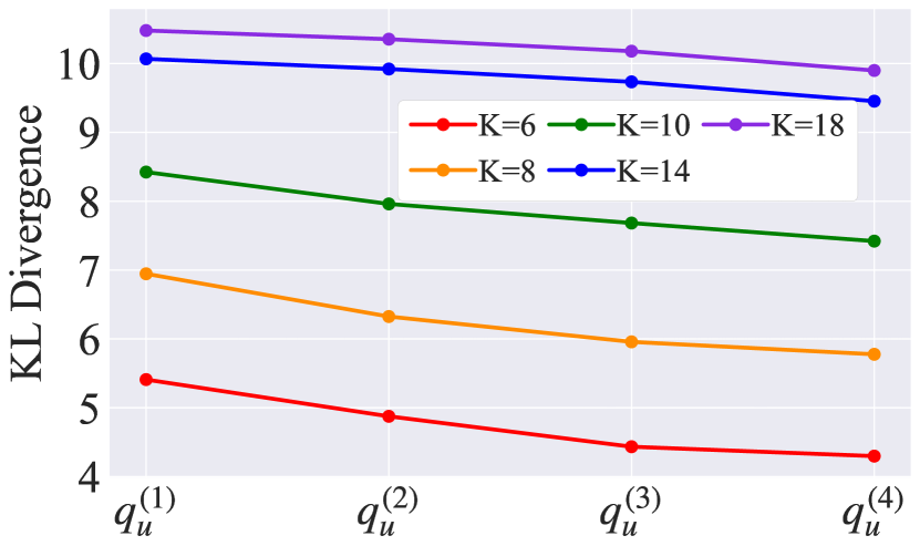
Figure 3. Visualization of consistency between user historical and predicted preference.

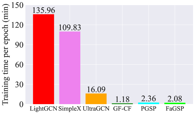
Figure 4. The average training time (5 times) of FaGSP and other methods on ML1M.

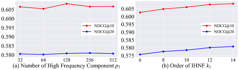
Figure 5. The sensitivity analysis of two hyper-parameters on ML1M dataset: Number of High Frequency Component $p_{1}$ and Order of Item High-order Neighborhood Filter (IHNF) $k_{1}$.

4.4. Visualization

We visualize the consistency between user historical preference distribution (calculated from training data) and user predicted preference distribution (calculated from model prediction) on ML100K to show that introducing IHF, UHNF and IHNF can improve the accuracy of user preference modeling. Specifically, we define user $u$’s historical preference distribution $p_{u}$ according to the categories (e.g., Comedy, Action) of items that he/she has interacted with:

(24) $$p_{u}(\text{category}=l)=\frac{C_{ul}}{\sum_{k=1}^{L}C_{uk}},$$

where $C_{ul}~{}(u=1,2,\cdots,M,~{}~{}~{}l=1,2,\cdots,L)$ represents the number of appearances of the $l$-th category in the user $u$’s interacted items, $M$ is the number of users, and $L$ is the number of categories.

Similarly, we can define user $u$’s predicted preference distributions from his/her predicted items in test using ILF as $q^{(1)}_{u}$, and that after introducing IHF, UHNF and IHNF sequentially on the basis of ILF as $q^{(2)}_{u}$ (i.e. ILF+IHF), $q^{(3)}_{u}$ (i.e. ILF+IHF+UHNF) and $q_{u}^{(4)}$ (i.e. ILF+IHF+UHNF+IHNF). Then we use the Kullback–Leibler (KL) divergence to evaluate the quality of the predicted preference distribution, where smaller KL divergence indicates better predicted preference distribution. The KL divergence between $p$ and $q$ is:

(25) $$\mathbf{KL}(p,q^{(w)})=\frac{1}{M}\sum_{u=1}^{M}\sum_{l=1}^{L}p_{u}(l)\ln\frac{p_{u}(l)}{q^{(w)}_{u}(l)},~{}w=1,2,3,4.$$

If $\mathbf{KL}(p,q^{(1)})>\mathbf{KL}(p,q^{(2)})$, it indicates that it is useful to introduce IHF, making the predicted preference distribution have a higher consistency with historical preference distribution.

Figure 5 shows the results of consistency between user historical preference and user predicted preference with respect to top-$K$ categories ($K\in\{6,8,10,14,18\}$) under different filter combinations. We can find that the KL divergence is constantly decreasing after introducing IHF, UHNF and IHNF sequentially on the basis of the ILF in all settings of $K$, which shows that IHF, UHNF and IHNF are all beneficial to restore user’s real interactive intentions by utilizing user/item unique characteristics and user and item high-order neighborhood information, making the predicted user preference as close as possible to user historical preference, thereby achieving accurate recommendation. Note that when $K$ increases, the decline magnitude of KL Divergence is decreasing, since several noisy categories at the tail affect the analysis of consistency.

4.5. Efficiency Analysis

We conduct the efficiency analysis on ML1M dataset by comparing the training time of FaGSP and other methods. For DGCF, LightGCN, SimpleX and UltraGCN which need back propagation to train the model, we accumulate the training time until we obtain the optimal validation accuracy. For GF-CF, PGSP and FaGSP, we directly calculate its training time, including the time for SVD.

Figure 5 shows the experimental results. From the results, we can find that compared with the GSP-based CF methods, FaGSP is comparable to GF-CF and PGSP. Compared with the GCN-based methods, FaGSP is 8X faster than that of UltraGCN, which is the most efficient GCN-based method among the baselines. Therefore, we can conclude that FaGSP is highly efficient.

4.6. Sensitivity Analysis

We conduct the sensitivity analysis on ML1M dataset to study how two important hyper-parameters affect the performance of FaGSP. The experimental results are shown in Figure 5, and we only show the results of NDCG@10 and NDCG@20 for better presentation of their trends, however, other metrics can draw the same conclusion.

4.6.1. Number of High Frequency Components $p_{1}$.

Figure 5 (a) shows that the accuracy of FaGSP first increases and then decreases as $p_{1}$ increases. This is because as $p_{1}$ increases, more unique characteristics are captured by FaGSP, thereby improving the accuracy of interaction prediction. However, noisy interactions also corresponds to high-frequency components, and excessive high-frequency components will also adopt the noisy interactions to model user preference, thereby affecting the accuracy of interaction prediction.

4.6.2. Order of Item High-order Neighborhood Filter $k_{1}$.

Figure 5 (b) shows as $k_{1}$ increases, the performance of the model has significantly improved, as more and more information from neighbors of different distances of item to be used to model user preference, thus improving the accuracy of recommendation results. However, an increase in $k_{1}$ will cause $(\mathbf{I}-\mathbf{O}_{I})^{k_{1}}$ to become dense, thereby increasing the computational complexity of FaGSP. Simultaneously, the performance gain of FaGSP is also gradually decreasing as $k_{1}$ becomes larger. Therefore, selecting an appropriate $k_{1}$ is necessary to balance the accuracy and running efficiency of the model. For the order of User High-order Neighborhood Filter $k_{2}$, we do not report it due to the space limitation but can draw the same conclusion.

5. Related Work

5.1. GCN-based Recommendation Algorithm

Recommender system, which studies the interactions between users and items, plays an important role in various domains, such as education (Obeid et al., 2018; Dwivedi and Roshni, 2017; Urdaneta-Ponte et al., 2021), medical (Tran et al., 2021; Katzman et al., 2018; De Croon et al., 2021) and e-commerce (Sarwar et al., 2002; Wei et al., 2007). Formally, user interactions can be constructed as a graph, where nodes are users and items, and edges are interactions between users and items. Due to the fact that graph convolutional networks (GCNs) has powerful structural feature extraction ability (Xu et al., [n. d.]; Zhang and Chen, 2018), more researchers begin to design recommendation algorithms based on GCNs, resulting in the rapid development of GCN-based recommendation algorithms (Ying et al., 2018; Wang et al., 2020; Wu et al., 2021b; Tian et al., 2022; Xia et al., 2022; Li et al., 2022; Wei et al., 2022). GCMC (Berg et al., 2018) is an early GCN-based recommendation algorithm that introduced a graph auto-encoder to reconstruct user historical interactions, so as to predict user future interactions. PinSage (Ying et al., 2018) combined random walks and graph convolutions to generate embeddings of items that incorporated both graph structure and node feature information, and designed a novel training strategy that relied on hard training examples to improve robustness and convergence of the model. UltraGCN (Mao et al., 2021b) proposed a simple yet effective GCN-based recommendation algorithm which resorted to approximate the limit of infinite-layer graph convolutions via a constraint loss and allowed for more appropriate edge weight assignments and flexible adjustment of the relative importance among different relationships.

It should be noted that the depth of GNN is restricted due to the over-smoothing problem (Chen et al., 2020a; Xu et al., 2018), where nodes tend to have similar representations. LR-GCCF (Chen et al., 2020b) introduced the skip connection (He et al., 2016) to alleviate the over-smoothing problem and made GNN deeper. IMP-GCN (Liu et al., 2021) proposed to propagate information in the user sub-graphs instead of the whole interaction graph, so as to reduce the impact of noise or negative information and alleviate the over-smoothing problem to make personalized recommendation.

5.2. GSP-based Recommendation Algorithm

GSP-based recommendation algorithms (Huang et al., 2017; Shen et al., 2021; Liu et al., 2023) are receiving increasing attention from researchers due to its parameter-free characteristic, making them highly efficient and able to achieve decent performance. GF-CF (Shen et al., 2021) developed a unified graph convolution-based framework and proposed a simple yet effective collaborative filtering method which integrated a linear filter and an ideal low-pass filter to make recommendation. PGSP (Liu et al., 2023) proposed a mixed-frequency low-pass filter over the personalized graph signal to model user preference and predict user interactions. However, these methods neglect to utilize user/item unique characteristics and user and item high-order neighborhood information to model user preference, making the modeled user preference sub-optimal.

6. Conclusion

We propose a frequency-aware graph signal processing method (FaGSP) for collaborative filtering to fully utilize information in user interactions for user future interaction prediction. FaGSP consists of a Cascaded Filter Module—which is composed of an ideal high-pass filter and an ideal low-pass filter—to take both user/item unique characteristics and common characteristics into consideration for user preference modeling, and a Parallel Filter Module—which is composed of two low-pass filters—to fully utilize user and item high-order neighborhood information for user preference modeling. Extensive experiments demonstrate the superiority of our method from the perspectives of recommendation accuracy and training efficiency compared to existing GCN/GSP-based CF methods.

References

- (1)
- Berg et al. (2018) Rianne van den Berg, Thomas N Kipf, and Max Welling. 2018. Graph convolutional matrix completion. In KDD Workshop on Deep Learning Day.
- Chen et al. (2020a) Deli Chen, Yankai Lin, Wei Li, Peng Li, Jie Zhou, and Xu Sun. 2020a. Measuring and relieving the over-smoothing problem for graph neural networks from the topological view. In Proceedings of the AAAI conference on artificial intelligence, Vol. 34. 3438–3445.
- Chen et al. (2020b) Lei Chen, Le Wu, Richang Hong, Kun Zhang, and Meng Wang. 2020b. Revisiting graph based collaborative filtering: A linear residual graph convolutional network approach. In Proceedings of the AAAI conference on artificial intelligence, Vol. 34. 27–34.
- Chung (1997) Fan RK Chung. 1997. Spectral graph theory. Vol. 92. American Mathematical Soc.
- De Croon et al. (2021) Robin De Croon, Leen Van Houdt, Nyi Nyi Htun, Gregor Štiglic, Vero Vanden Abeele, and Katrien Verbert. 2021. Health recommender systems: systematic review. Journal of Medical Internet Research 23, 6 (2021), e18035.
- Dong et al. (2020) Xiaowen Dong, Dorina Thanou, Laura Toni, Michael Bronstein, and Pascal Frossard. 2020. Graph signal processing for machine learning: A review and new perspectives. IEEE Signal processing magazine 37, 6 (2020), 117–127.
- Dwivedi and Roshni (2017) Surabhi Dwivedi and VS Kumari Roshni. 2017. Recommender system for big data in education. In 2017 5th National Conference on E-Learning & E-Learning Technologies (ELELTECH). IEEE, 1–4.
- He et al. (2016) Kaiming He, Xiangyu Zhang, Shaoqing Ren, and Jian Sun. 2016. Deep residual learning for image recognition. In Proceedings of the IEEE conference on computer vision and pattern recognition. 770–778.
- He et al. (2020) Xiangnan He, Kuan Deng, Xiang Wang, Yan Li, Yongdong Zhang, and Meng Wang. 2020. Lightgcn: Simplifying and powering graph convolution network for recommendation. In Proceedings of the 43rd International ACM SIGIR conference on research and development in Information Retrieval. 639–648.
- Huang et al. (2017) Weiyu Huang, Antonio G Marques, and Alejandro Ribeiro. 2017. Collaborative filtering via graph signal processing. In 2017 25th European signal processing conference (EUSIPCO). IEEE, 1094–1098.
- Katzman et al. (2018) Jared L Katzman, Uri Shaham, Alexander Cloninger, Jonathan Bates, Tingting Jiang, and Yuval Kluger. 2018. DeepSurv: personalized treatment recommender system using a Cox proportional hazards deep neural network. BMC medical research methodology 18, 1 (2018), 1–12.
- Kipf and Welling (2017) Thomas N Kipf and Max Welling. 2017. Semi-Supervised Classification with Graph Convolutional Networks. In International Conference on Learning Representations.
- Li et al. (2022) Anchen Li, Bo Yang, Huan Huo, and Farookh Hussain. 2022. Hypercomplex graph collaborative filtering. In Proceedings of the ACM Web Conference 2022. 1914–1922.
- Li et al. (2019) Xiaocan Li, Shuo Wang, and Yinghao Cai. 2019. Tutorial: Complexity analysis of singular value decomposition and its variants. arXiv preprint arXiv:1906.12085 (2019).
- Liu et al. (2021) Fan Liu, Zhiyong Cheng, Lei Zhu, Zan Gao, and Liqiang Nie. 2021. Interest-aware message-passing gcn for recommendation. In Proceedings of the Web Conference 2021. 1296–1305.
- Liu et al. (2023) Jiahao Liu, Dongsheng Li, Hansu Gu, Tun Lu, Peng Zhang, Li Shang, and Ning Gu. 2023. Personalized Graph Signal Processing for Collaborative Filtering. In Proceedings of the ACM Web Conference 2023. 1264–1272.
- Mao et al. (2021a) Kelong Mao, Jieming Zhu, Jinpeng Wang, Quanyu Dai, Zhenhua Dong, Xi Xiao, and Xiuqiang He. 2021a. SimpleX: A simple and strong baseline for collaborative filtering. In Proceedings of the 30th ACM International Conference on Information & Knowledge Management. 1243–1252.
- Mao et al. (2021b) Kelong Mao, Jieming Zhu, Xi Xiao, Biao Lu, Zhaowei Wang, and Xiuqiang He. 2021b. UltraGCN: ultra simplification of graph convolutional networks for recommendation. In Proceedings of the 30th ACM International Conference on Information & Knowledge Management. 1253–1262.
- Obeid et al. (2018) Charbel Obeid, Inaya Lahoud, Hicham El Khoury, and Pierre-Antoine Champin. 2018. Ontology-based recommender system in higher education. In Companion proceedings of the the web conference 2018. 1031–1034.
- Ortega et al. (2018) Antonio Ortega, Pascal Frossard, Jelena Kovačević, José MF Moura, and Pierre Vandergheynst. 2018. Graph signal processing: Overview, challenges, and applications. Proc. IEEE 106, 5 (2018), 808–828.
- Pang et al. (2023) Shanchen Pang, Kuijie Zhang, Gan Wang, Jerry Chun-Wei Lin, Fuyu Wang, Xiangyu Meng, Shudong Wang, and Yuanyuan Zhang. 2023. AF-GCN: Completing various graph tasks efficiently via adaptive quadratic frequency response function in graph spectral domain. Information Sciences 623 (2023), 469–480.
- Paterek (2007) Arkadiusz Paterek. 2007. Improving regularized singular value decomposition for collaborative filtering. In Proceedings of KDD cup and workshop, Vol. 2007. 5–8.
- Sarwar et al. (2002) Badrul M Sarwar, George Karypis, Joseph Konstan, and John Riedl. 2002. Recommender systems for large-scale e-commerce: Scalable neighborhood formation using clustering. In Proceedings of the fifth international conference on computer and information technology, Vol. 1. 291–324.
- Shen et al. (2021) Yifei Shen, Yongji Wu, Yao Zhang, Caihua Shan, Jun Zhang, B Khaled Letaief, and Dongsheng Li. 2021. How powerful is graph convolution for recommendation?. In Proceedings of the 30th ACM international conference on information & knowledge management. 1619–1629.
- Song et al. (2010) Jinbo Song, Chao Chang, Fei Sun, Xinbo Song, and Peng Jiang. 2010. NGAT4Rec: Neighbor-Aware Graph Attention Network For Recommendation (2020). arXiv preprint arXiv:2010.12256 (2010).
- Spielman (2007) Daniel A Spielman. 2007. Spectral graph theory and its applications. In 48th Annual IEEE Symposium on Foundations of Computer Science (FOCS’07). IEEE, 29–38.
- Stanković et al. (2019) Ljubiša Stanković, Miloš Daković, and Ervin Sejdić. 2019. Introduction to graph signal processing. Vertex-Frequency Analysis of Graph Signals (2019), 3–108.
- Sun et al. (2020) Jianing Sun, Yingxue Zhang, Wei Guo, Huifeng Guo, Ruiming Tang, Xiuqiang He, Chen Ma, and Mark Coates. 2020. Neighbor interaction aware graph convolution networks for recommendation. In Proceedings of the 43rd international ACM SIGIR conference on research and development in information retrieval. 1289–1298.
- Tian et al. (2022) Changxin Tian, Yuexiang Xie, Yaliang Li, Nan Yang, and Wayne Xin Zhao. 2022. Learning to denoise unreliable interactions for graph collaborative filtering. In Proceedings of the 45th International ACM SIGIR Conference on Research and Development in Information Retrieval. 122–132.
- Tran et al. (2021) Thi Ngoc Trang Tran, Alexander Felfernig, Christoph Trattner, and Andreas Holzinger. 2021. Recommender systems in the healthcare domain: state-of-the-art and research issues. Journal of Intelligent Information Systems 57 (2021), 171–201.
- Urdaneta-Ponte et al. (2021) María Cora Urdaneta-Ponte, Amaia Mendez-Zorrilla, and Ibon Oleagordia-Ruiz. 2021. Recommendation systems for education: systematic review. Electronics 10, 14 (2021), 1611.
- Wang et al. (2020) Xiang Wang, Hongye Jin, An Zhang, Xiangnan He, Tong Xu, and Tat-Seng Chua. 2020. Disentangled graph collaborative filtering. In Proceedings of the 43rd international ACM SIGIR conference on research and development in information retrieval. 1001–1010.
- Wei et al. (2022) Chunyu Wei, Jian Liang, Bing Bai, and Di Liu. 2022. Dynamic hypergraph learning for collaborative filtering. In Proceedings of the 31st ACM International Conference on Information & Knowledge Management. 2108–2117.
- Wei et al. (2007) Kangning Wei, Jinghua Huang, and Shaohong Fu. 2007. A survey of e-commerce recommender systems. In 2007 international conference on service systems and service management. IEEE, 1–5.
- Wu et al. (2021a) Jiancan Wu, Xiang Wang, Fuli Feng, Xiangnan He, Liang Chen, Jianxun Lian, and Xing Xie. 2021a. Self-supervised graph learning for recommendation. In Proceedings of the 44th international ACM SIGIR conference on research and development in information retrieval. 726–735.
- Wu et al. (2021b) Jiancan Wu, Xiang Wang, Fuli Feng, Xiangnan He, Liang Chen, Jianxun Lian, and Xing Xie. 2021b. Self-supervised graph learning for recommendation. In Proceedings of the 44th international ACM SIGIR conference on research and development in information retrieval. 726–735.
- Xia et al. (2022) Lianghao Xia, Chao Huang, Yong Xu, Jiashu Zhao, Dawei Yin, and Jimmy Huang. 2022. Hypergraph contrastive collaborative filtering. In Proceedings of the 45th International ACM SIGIR conference on research and development in information retrieval. 70–79.
- Xu et al. ([n. d.]) Keyulu Xu, Weihua Hu, Jure Leskovec, and Stefanie Jegelka. [n. d.]. How Powerful are Graph Neural Networks?. In International Conference on Learning Representations.
- Xu et al. (2018) Keyulu Xu, Chengtao Li, Yonglong Tian, Tomohiro Sonobe, Ken-ichi Kawarabayashi, and Stefanie Jegelka. 2018. Representation learning on graphs with jumping knowledge networks. In International conference on machine learning. PMLR, 5453–5462.
- Ying et al. (2018) Rex Ying, Ruining He, Kaifeng Chen, Pong Eksombatchai, William L Hamilton, and Jure Leskovec. 2018. Graph convolutional neural networks for web-scale recommender systems. In Proceedings of the 24th ACM SIGKDD international conference on knowledge discovery & data mining. 974–983.
- Yu and Qin (2020) Wenhui Yu and Zheng Qin. 2020. Graph convolutional network for recommendation with low-pass collaborative filters. In International Conference on Machine Learning. PMLR, 10936–10945.
- Zhang and Chen (2018) Muhan Zhang and Yixin Chen. 2018. Link prediction based on graph neural networks. Advances in neural information processing systems 31 (2018).