Conditional Neural Expert Processes for Learning from Demonstration

Abstract

Learning from Demonstration (LfD) is a widely used technique for skill acquisition in robotics. However, demonstrations of the same skill may exhibit significant variances, or learning systems may attempt to acquire different means of the same skill simultaneously, making it challenging to encode these motions into movement primitives. To address these challenges, we propose an LfD framework, namely the Conditional Neural Expert Processes (CNEP), that learns to assign demonstrations from different modes to distinct expert networks utilizing the inherent information within the latent space to match experts with the encoded representations. CNEP does not require supervision on which mode the trajectories belong to. Provided experiments on artificially generated datasets demonstrate the efficacy of CNEP. Furthermore, we compare the performance of CNEP with another LfD framework, namely Conditional Neural Movement Primitives (CNMP), on a range of tasks, including experiments on a real robot. The results reveal enhanced modeling performance for movement primitives, leading to the synthesis of trajectories that more accurately reflect those demonstrated by experts, particularly when the model inputs include intersection points from various trajectories. Additionally, CNEP offers improved interpretability and faster convergence by promoting expert specialization. Furthermore, we show that the CNEP model accomplishes obstacle avoidance tasks with a real manipulator when provided with novel start and destination points, in contrast to the CNMP model, which leads to collisions with the obstacle.

I Introduction

The capability of robots to comprehend and respond to dynamic environments is vital for their integration across various contexts. Specifically, most real-world tasks require the robots to model and construct spatiotemporal sensorimotor trajectories. Early applications involved manually recording the sensorimotor information generated by a demonstrator on a teleoperated robot and, later, autonomously following them on the robot [1]. A skill was then represented by a series of primitive action segments selected according to simple conditional rules. These manually recorded controllers often fail outside the controlled environments due to the inherent characteristics of real-world environments as explained in [2].

Nowadays, adaptability and generalizability have been the cornerstone objectives in robotics research. These requirements have transformed the skill acquisition procedures by necessitating the incorporation of data-driven approaches. To this end, Learning from Demonstration (LfD) is a widely adopted procedure in robotics that enables learning controllers to acquire new skills by observing an expert [3, 4]. For this purpose, elaborate demonstrations of target skills are required in LfD. On the other hand, the set of expert demonstrations for a particular real-world skill may contain significant variances, or there might be multiple ways to achieve the same skill. These variances reflect the stochastic nature of the expert demonstrations, which poses the challenge of handling quantitatively and qualitatively different demonstrations for LfD-based skill-acquisition procedures.

In this study, we introduce the Conditional Neural Expert Processes (CNEP) model, which is a generic and monolithic LfD framework to teach robots the necessary controllers to model and synthesize complex, multimodal sensorimotor trajectories. In previous approaches, such as [5, 6, 7, 8], the multimodality aspect of target skills was not explicitly addressed as these approaches attempted to represent different modes with the same mechanism, leading to a seamless interpolation inside the demonstration space, which may lead to suboptimal behavior, as shown in [9]. On the contrary, our CNEP is designed to model different modes in the demonstrations with different experts and generate the required motion trajectory by automatically selecting the corresponding expert. Our model is built on top of Conditional Neural Movement Primitives (CNMP) [8], which was shown to form robust representations to model complex motion trajectories from a few data points. CNMPs have an encoder-decoder structure that allows them to generate motion trajectories given several conditioning (observation) points. CNEP uses multiple decoders (experts) - instead of a single one - that are responsible for different modes in the given trajectories. Given the conditioning points and the output of the encoder network, a novel gating mechanism assigns probabilities to the experts, and the decoder with the highest probability is used to generate the motion trajectory from the encoded conditioning points.

Besides the architectural contribution that includes the gating mechanism and multiple experts, we propose a novel loss function composed of three components. The first component is the reconstruction loss, which is calculated based on the difference between the predictions of the experts and the ground truth, following [8]. The second and the third elements of the loss function are novel components that are used to ensure that all the experts are evenly utilized and an expert, when assigned, is selected with high probability. These objectives are achieved by minimizing the entropy of expert assignments for the conditioning points of a single trajectory and maximizing the entropy of expert assignments for the complete batch.

We evaluated our system using different sets of artificially generated trajectories and motion trajectories from a real robot system. We showed that our CNEP outperforms the baseline CNMP model when the number of modes in the demonstrations increases when the systems are required to generate trajectories from common points of several demonstrations and when generalizing into unseen conditioning points.

This paper unfolds as follows: Section II reviews the related work in sensorimotor trajectory modeling, which enables modeling and synthesizing motion trajectories. Section III outlines the methodology of the CNEP procedure, explaining the structures and functions of the individual components. Section IV presents experimental results, establishing the effectiveness of CNEP in handling multimodal data. Finally, Section V offers concluding remarks and potential future directions.

II Related Work

Equipping robots with the desired skills has been the driving force in robotics research. In initial studies, controllers with precise mathematical representations were used. These representations were formed using the physics-based dynamic models of the environment and the kinematic models of the agents [10]. Although accurate in controlled settings and computationally less intense, the applicability of the precise models was limited in realistic scenarios. This is mainly due to their constrained flexibility in the kinodynamic space of the system, preventing the generalization of acquired skills into novel conditions.

To create more flexible controllers, one popular LfD framework in recent years has been Dynamic Movement Primitives (DMP) [5]. In DMPs, expert demonstrations of complex skills are encoded with a system of differential equations in the form of movement primitives. DMPs can be queried upon modeling to generate motion trajectories from start to end. Also, when integrated with closed-loop feedback, DMPs are proven suitable for real-time control as they adapt to changes and perturbations in real-time, offering robust performance in many applications [11]. On the other hand, only a single trajectory can be encoded by the classical DMP formulation, indicating that variabilities inside demonstrations are not considered.

Probabilistic approaches have been proposed to address the abovementioned requirements by offering flexible and robust modeling mechanisms. In this respect, Gaussian Mixture Models (GMM) and Hidden Markov Models (HMM) have been used in several studies [12, 13, 14] to capture the variability of the task by learning the distributions of the demonstration data. The complexity of training and inference in HMMs increases as the dimensionality of the demonstrations increases, whereas variants of GMMs work well with high-dimensional data [15]. Nonetheless, when the demonstration data of the task is sampled from a multimodal distribution, GMMs fail to select one of the modes. In contrast, state-transition probabilities of HMMs encode this information, enabling the synthesis of expert-like trajectories [16]. The proposed CNEP addresses both of these issues. It utilizes multiple expert networks to handle multimodal data and can work with high-dimensional raw data coming directly from the sensors.

As stated in [17, 18], the uncertainty in real-world tasks has been explicitly addressed by the use of Gaussian Processes (GPs). As a result, the computational efficiency of learning adaptable and robust robotic controllers is improved to enable control in real-world tasks. Pure GP approaches are known to work well in Euclidean spaces. However, when the demonstration data displays non-Euclidean characteristics, such as rotation of robotic joints, further adjustments are required for GP methods [19]. This is not the case for CNEP as illustrated with the real robot tests where the complete trajectories in the non-Euclidean joint space are used as demonstrations.

Addressing the in-task variability, Probabilistic Motion Primitives (ProMP) have been proposed to encode a distribution of trajectories [20]. In [6], ProMPs were shown to provide improved generalization capabilities, enabling generated trajectories to be adapted so that they could pass through desired via points. However, due to their formulation, they fail when the demonstration set does not match a Gaussian distribution. Furthermore, the use of basis functions limits the applicability of this method to high-dimensional data.

In recent years, owing to the advances in machine learning, deep learning methods have been employed to offer alternatives to manual approaches. LSTMs have been successfully used in various studies to learn and generate multimodal trajectories [21]. Despite their success compared to the earlier methods, vast amounts of data are required to train LSTMs. Moreover, they are fed on their predictions to make further predictions, which induces an accumulated error problem in long-horizon predictions [22]. Contrarily, CNEP can be queried to generate long-horizon trajectories without an error-accumulation issue.

As a deep LfD framework, Conditional Neural Movement Primitives (CNMP) is developed based on Conditional Neural Processes (CNP) [7], also aiming to handle high-dimensional sensorimotor data. The ability of CNMP to use raw visual data is illustrated by the integration of a Convolutional Neural Network as a state encoder [8]. In short, CNMP can be used to learn robust representations about the underlying patterns in the sensorimotor data and construct trajectories that can be conditioned on real-time sensory data to enable real-time responses. It has been successfully applied to complex trajectory data across numerous studies and domains, such as [23, 24]. However, only a single query network is used in CNMP to decode different demonstrations of a movement primitive. As a result, trajectories are formed by interpolating between different modes of the same skill, which may lead to suboptimal results where the demonstration trajectories are multimodal or intersecting.

III Method

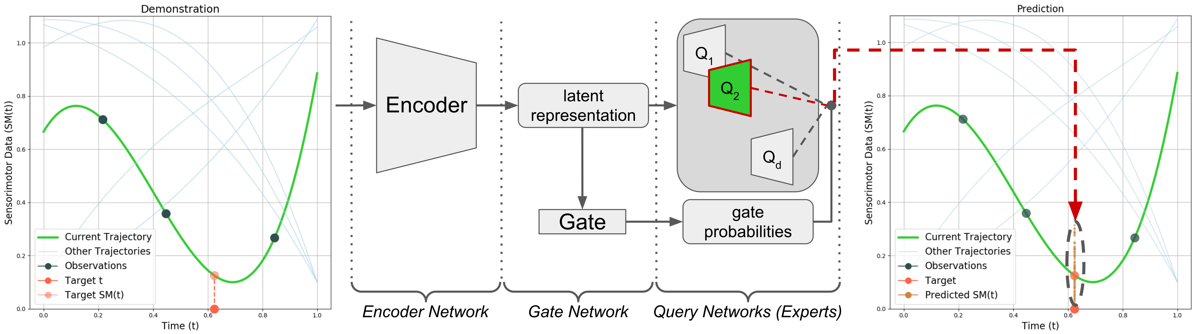
Figure 1: The CNEP model contains an Encoder, a Gate, and multiple Query Networks called experts. In this example, n=3 observation points (shown with $\bullet$) and m=1 target timepoints (shown with $\bullet$) are randomly sampled on the input trajectory. The latent representation, the mean of $n$ observation encodings, is used by: (1) the Gate Network to find the responsible expert and (2) expert networks to generate their predictions as normal distributions at the target timepoint. Refer to Section III-C1 for details.

III-A Problem Formulation

The skill-acquisition problem can be formulated as finding a sequence of motion commands that produce the desired movement [25]. Formally, the LfD system is expected to learn a function $\tau=f(t;X)$, where X denotes specific criteria, such as the starting point at $t=0$ or the destination at any time $t$, using N expert demonstrations, $D=\{\tau_{1},\tau_{2},\dotsc,\tau_{N}\}$. Despite the multimodality of the target skill, a resource-efficient solution with few demonstrations is also demanded to promote the applicability of the proposed approach in real-world settings where it is infeasible to provide so many demonstrations.

In this context, sensorimotor functions (SM(t)) are utilized to refer to the temporal mapping of sensory inputs and motor outputs of a robot at time t. Two important notions are encapsulated in the SM(t) formalism: (1) how a robot senses its environment through sensors and (2) how it responds through actuators at any given moment. The perspective of representing complex skills as SM(t) trajectories transforms skill-acquisition efforts into trajectory modeling and generation problems. A trajectory is formally defined as a temporal function, $\tau=\tau(t)$ following [26]. Throughout this study, each trajectory $\tau$ is represented as an ordered list of sensorimotor values; $\tau=\{SM(t_{1}),SM(t_{2}),\dotsc,SM(t_{T})\}$.

In the following, after introducing the baseline (CNMP) method, we provide details of our proposed method (CNEP). As LfD frameworks, both are used to encode a set of trajectories from expert demonstrations. They take a set of observation (conditioning) points, in the form of (t, SM(t)) tuples from a trajectory, and are expected to output the SM$(t_{q})$ value of any target timepoint, $t_{q}$. In practice, given varying observation points, the entire trajectory is generated by querying the system for all time points from $t_{1}$ to $t_{T}$.

III-B Background: CNMP

CNMP, introduced in [8], contains an Encoder and a Query Network. At the training time, a trajectory $\tau_{i}$ is first sampled from demonstrations, $D$. $n$ randomly sampled observation points from this trajectory are passed through the Encoder Network to generate corresponding latent representations. An averaging operation is applied to obtain a compact representation of the (n) input observations in the latent space. The average representation is then concatenated with $m$ random target timepoints and passed through the Query Network to output the distributions that describe the sensorimotor responses of the system at corresponding target timepoints. Here, $n$ and $m$ are random numbers, where $1\leq n\leq n_{max}$ and $1\leq m\leq m_{max}$. $n_{max}$ and $n_{max}$ are hyperparameters whose values are set empirically. The output is a multivariate normal distribution with parameters $(\mu_{q},\Sigma_{q})$. The loss is calculated as the negative log-likelihood of the ground-truth value under the predicted distribution as follows:

$$\mathcal{L}=-\>log\>P(\>\textit{SM}(t_{q})\>|\>\mathcal{N}(\mu_{q},\>softplus(\Sigma_{q})\>)\>).$$ (1)

This loss is backpropagated, updating the weights of both the Encoder and the Query networks. More details can be found in [8].

III-C Proposed Approach: CNEP

III-C1 Architecture Overview

The proposed architecture and the workflow are illustrated in Fig. 1. Similar to the CNMP, the input to the system is composed of $n$ observations, which are passed through the Encoder Network to generate the latent representation. The latent representation is fed into our novel Gate Network to produce the gate probabilities for all experts. Simultaneously, they are concatenated with $m$ target timepoints and are passed through all experts to generate $SM$ predictions at target timepoints. During training, the Gate Network’s output is combined with the experts’ outputs to compute the overall loss. After training, when the system is asked to generate a response for a target, only the prediction of the expert with the highest gate probability is outputted. An example case is shown in Fig. 1, where after producing the latent representation for n=3 observation points, the gating mechanism outputs a relatively high probability for the second expert, appointing it as the most confident expert for this query. Therefore, its response for m=1 target timepoint is selected as the output of the entire system. The system is trained end-to-end, as detailed in the next section.

III-C2 Training Procedure

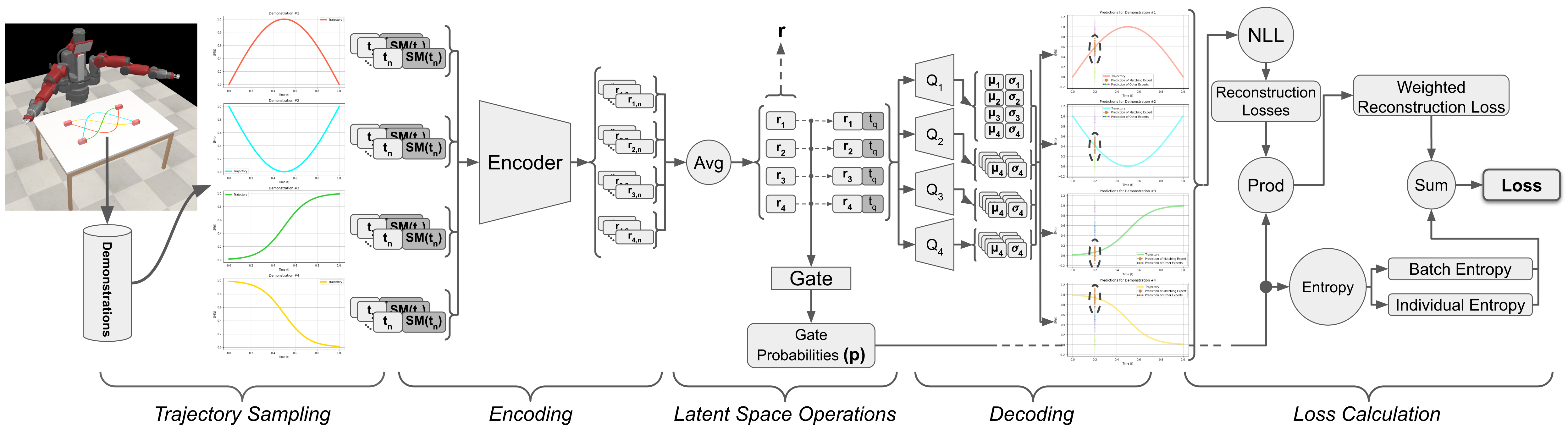
Figure 2: Initially, observation points from the input trajectory are mapped to the latent space by the Encoder Network. The averaged representations ($\mathbf{r}$) are (1) fed into the Gate Network and (2) concatenated with target points ($\mathbf{r_{q}}$) and fed into the Query Networks. While the candidate predictions are outputted by all Query Networks, the probabilities for each trajectory-expert pair ($\mathbf{p}$) are generated by the Gate Network. These probabilities are used in calculating the values of loss components as explained in Section III-C2.

The training phase of the CNEP model is depicted in Fig. 2. From a randomly selected trajectory, $\tau_{i}$, $n$ observation points are randomly sampled to form $(t,\textit{SM}(t))$ tuples and given to the Encoder Network. A compact representation estimate for $\tau_{i}$, $\mathbf{r_{i}}$, is obtained by averaging the output of the Encoder Network for the $n$ conditioning points. In Fig. 2, parallel processing of a batch of trajectories is shown.

Calculating Gate Probabilities, ($\mathbf{p}$)

The latent representation of a trajectory, $\mathbf{r_{i}}$, is fed into the Gate Network, which outputs the gate probabilities, $\mathbf{p_{i}}\in\mathbb{R}^{d}$, where $d$ is a hyperparameter of the model, denoting the number of experts. $\mathbf{p_{i}}$ is a $d$-dimensional probability distribution, indicating the confidence level of each expert ($Q_{e}$) for the latent representation $\mathbf{r_{i}}$, for $1\leq e\leq d$.

The Reconstruction Loss

Each expert predicts a normal distribution for the SM values at target timepoints, and a reconstruction loss is calculated using the ground-truth SM values. For this, $m$ target timepoints ($\mathbf{t_{q}}$) are randomly sampled, where m is set to 1 in Fig. 2 for simplicity. An $(\mathbf{r_{i}},\mathbf{t_{q}})$ tuple is passed through all experts ($Q_{e}$s) to generate their predictions. The negative log-likelihood of the actual $SM(\mathbf{t_{q}})$ under predicted distribution is computed as the reconstruction loss of the corresponding expert as follows:

$$L_{e}=-\>log\>P(\>\textit{SM}(\mathbf{t_{q}})\>|\>\mathcal{N}(\mathbf{\mu_{e}},\>softplus(\mathbf{\Sigma_{e}})\>)\>)$$

where $\mathbf{\mu_{e}}$ and $\mathbf{\Sigma_{e}}$ are the outputs of the Query Network, $Q_{e}$.

Next, the combined reconstruction loss for the trajectory $\tau_{i}$ is calculated by taking the weighted sum of $L_{e}$s of all experts:

$$\mathcal{L}_{rec}^{i}=\frac{1}{d}\sum_{e=1}^{d}L_{e}\times p_{i,e}$$

where $p_{i,e}$ is the probability of expert $e$ for the latent representation $\mathbf{r_{i}}$. For a batch of trajectories as shown in Fig. 2, the weighted reconstruction loss $\mathcal{L}_{rec}$ is the mean $\mathcal{L}_{rec}^{i}$, where $1\leq i\leq b$, and b is the batch size.

Expert Assignment Losses

We would like our system to avoid selecting the same expert for all possible modes. For this purpose, the entropy of the expert activation frequencies over a batch of training trajectories should be maximized. We use batch entropy ($\mathcal{L}_{\textrm{batch}}$) to enforce this constraint. In the meantime, we would like the system to have high confidence in assigning an $(\mathbf{r_{i}},\mathbf{t_{q}})$ tuple to one of the experts. For this, the entropy of the gate probabilities, $p_{i}$, should be minimized. We use individual entropy ($\mathcal{L}_{ind}$) to enforce this constraint.

Formally, $\mathcal{L}_{\textrm{batch}}\in\mathbb{R}$ is calculated as follows:

$$\mathcal{L}_{\textrm{batch}}=-\sum_{e=1}^{d}\left(\frac{1}{b}\sum_{i=1}^{b}p_{i,e}\right)\log\left(\frac{1}{b}\sum_{i=1}^{b}p_{i,e}\right)$$

where, again, $b$ is batch size, and $d$ is the number of experts.

Subsequently, $\mathcal{L}_{ind}\in\mathbb{R}$ is computed as follows:

$$\mathcal{L}_{ind}=\frac{1}{b}\sum_{i=1}^{b}\left(-\sum_{e=1}^{d}p_{i,e}\log(p_{i,e})\right)$$

The entire system is trained in an end-to-end manner where the parameters of the Encoder, the Gate, and the Query Networks are trained simultaneously in a supervised way. The overall loss function is a linear combination of the abovementioned three components: 1) the weighted reconstruction loss, 2) batch-wise expert activation loss, the batch entropy, and 3) trajectory-wise confidence of expert selection, the individual entropy. The dynamic nature of expert selection necessitates careful handling during training to achieve the right balance between expert adaptation and overall system stability. Essentially, as the model attempts to decrease the reconstruction loss, it stimulates experts to make accurate predictions. Moreover, while the model attempts to increase batch entropy, it promotes expert specialization by preventing the overutilization of any expert. Lastly, the individual entropy component of the loss indicates the confidence of latent representation-expert matching. As the model attempts to decrease this value, it contributes to the specialization of experts by assigning similar representations to the same expert. As a result, the following overall loss function is used:

$$\mathcal{L}_{total}=\alpha_{1}*\mathcal{L}_{rec}+\alpha_{2}*\mathcal{L}_{batch}+\alpha_{3}*\mathcal{L}_{ind},$$ (2)

where weighting coefficients of these components, $\alpha_{1}$, $\alpha_{2}$, and $\alpha_{3}$, are found empirically by the grid search technique using a specific library, called Weights & Biases, [27].

III-C3 PID Controller

To execute learned skills on the robot, a PID controller is appended to the end of our system, ensuring that synthesized trajectories pass through specified observation points. The predicted SM trajectories are fed into this controller prior to the execution. The control signal $u(t)$ for each timestep is calculated using the PID formula:

$$\mathbf{u}(t)=K_{p}\cdot\mathbf{e}(t)+K_{i}\cdot\int\mathbf{e}(t)\,dt+K_{d}\cdot\frac{d}{dt}\mathbf{e}(t)$$

where $\mathbf{e}(t)$ is the error vector at time $t$, and $K_{p}$, $K_{i}$, and $K_{d}$ are the proportional, integral, and derivative gains, respectively, which define the controller’s behavior.

The error $\mathbf{e}(t)$ is the difference between the current point and the conditioning point. A decay mechanism of certain timesteps is incorporated into the error calculation. This ensures that the corrections diminish, allowing the trajectory to converge smoothly toward the desired path.

IV Experiments and Results

This section provides an experimental evaluation of the CNEP model in various tests. First, multiple sets of synthetically produced oscillatory curves are used as sensorimotor trajectories to simulate different means of achieving the same sensorimotor skill. Later, with another set of artificially generated trajectories, the proposed model is assessed against an ensemble of movement primitives. Experiments with synthetically generated demonstrations are conducted to provide controlled environments for a quantitative assessment. Finally, the proposed approach is evaluated on a real-world obstacle-avoidance task of a robotic manipulator. In this task, different paths are provided by a demonstrator to avoid an obstacle in the task space. Eventually, the model’s efficacy and applicability in practical settings are demonstrated by this experiment. While conducting these tests, the CNEP method is compared with a baseline, the CNMP method from the following angles: learning curves, validation errors, and generalization capabilities.

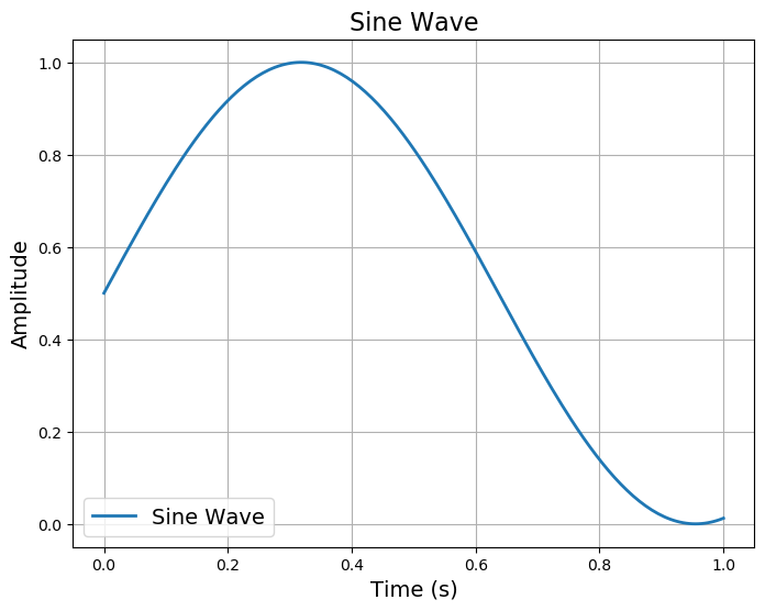
(a)

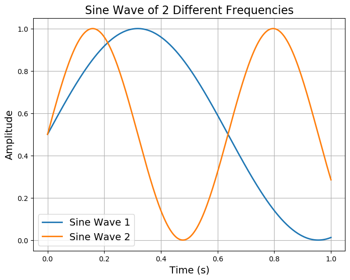
(b)

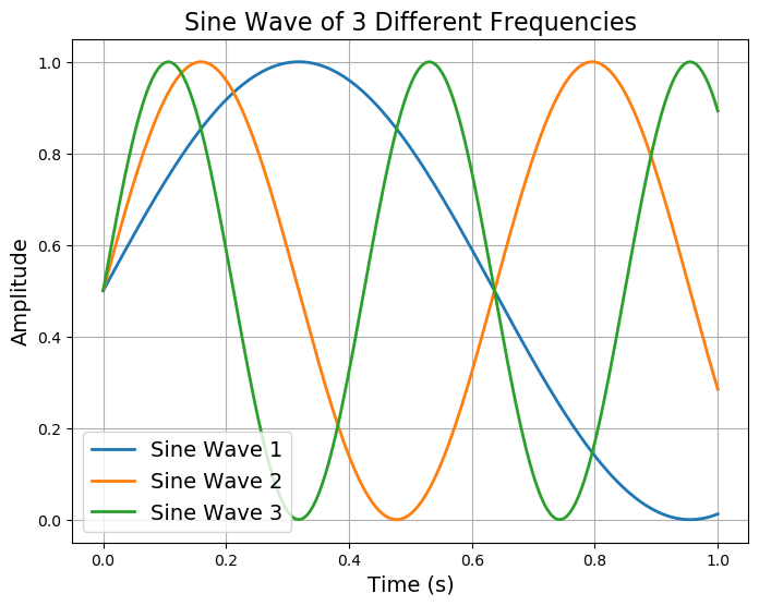
(c)

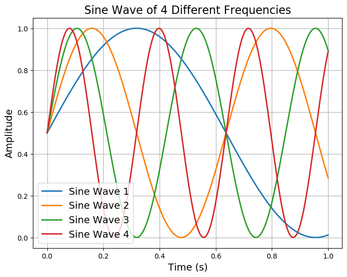
(d)

Figure 3: Distinct datasets with sine waves of different frequencies are generated. Each dataset is used in a distinct comparison between CNEP and CNMP models. Learning from one of these datasets becomes more challenging as the number of modalities increases.

In each comparison, despite the existence of multiple Query Networks in CNEP, careful consideration was given to maintaining a marginally larger overall size for the CNMP model than for the CNEP model, ensuring a fair comparison. Furthermore, all other factors, including optimizer parameters, datasets, training durations, etc., were kept constant. Various performance metrics are encompassed in the evaluation, shedding light on CNEP’s potential for trajectory prediction and specialization. Additionally, the outcomes are again compared with CNMP to establish the advancements offered by the proposed method.

IV-A Trajectory Datasets with Increasing Complexities

In this section, the performance of our method is evaluated and compared to the baseline CNMP model when the complexity of the skill dataset is gradually increased. For this purpose, four datasets that are composed of 1, 2, 3, and 4 trajectories are prepared. These trajectories correspond to sine waves of varying frequencies, as shown in Fig. 3. Here, the y-axis represents SM values, and the x-axis represents the time. Note that the sine function is used just as an example to generate different types of trajectories, which can be replaced with other functions. The two models, CNEP and CNMP, are trained separately on each dataset. The number of parameters in both models is kept close for a fair comparison.

To measure the performance, full-length trajectories are regenerated during the validation phase of the training. The Mean-Squared Error (MSE) is used to measure the distance between reconstructed trajectories and demonstrations. Similar reconstruction errors are calculated for both models when the dataset comprises demonstrations from a single mode, as shown in Fig. 4a. On the other hand, the performance of the CNEP starts outperforming the baseline CNMP model when the demonstration dataset becomes multimodal due to its gated formulation and the automatic selection of experts. Furthermore, the difference in performance between CNEP and CNMP becomes more significant as the number of modes increases. As shown in Fig. 4b, CNEP also achieves faster convergence.

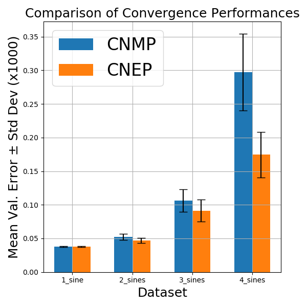
(a)

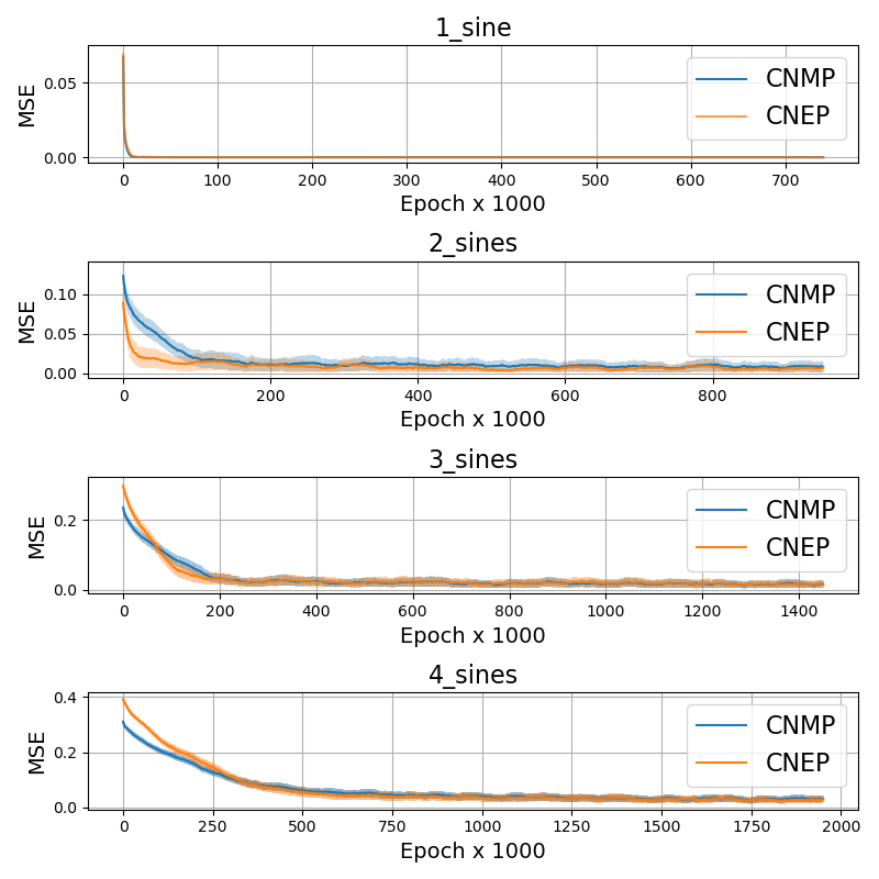
(b)

Figure 4: Comparison of learning performances of the two approaches. In (a), the mean validation errors over 30 runs are given. Fewer reconstruction errors are produced by CNEP (shown in orange) than by CNMP (shown in blue). Mean training losses, which are plotted in (b), indicate that convergence is achieved faster by CNEP.

IV-B Modelling Significantly Different Trajectories with Common Points

When showing skill with diverse demonstrations, the corresponding trajectories probably pass through the same points. For example, consider a scenario where the arm is required to execute different point-to-point movements while passing through common apertures between obstacles. It is challenging for LfD systems to generate correct SM values when only conditioned from these intersecting points. In this section, we aim to evaluate the performance of our model and compare it with the baseline when distinct trajectories with several common points are required to be learned. Both CNEP and CNMP are trained with the dataset of four SM trajectories shown in Fig. 5a, where the trajectories intersect at various points. Here, we aim to evaluate the performance of our model when it is required to generate the trajectory given observation points close to the common points. For this purpose, the models are conditioned with points from the shaded regions shown in Fig. 5b.

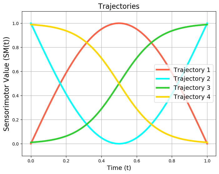
(a)

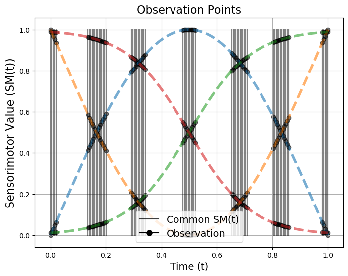
(b)

Figure 5: In (a), the SM trajectories for four distinct trajectories are plotted, intersecting at several points and presenting a challenging decision for models conditioned on these intersections. In (b), observation points used in the comparison are sampled from the shaded regions.

Fig. 6b compares the performances of CNEP and CNMP models. When these models are conditioned from points that do not correspond to an intersection point, both models generate the required trajectories successfully, as shown on the top row of Fig. 6a. However, when they are conditioned from intersection points, CNMP fails, whereas CNEP successfully generates the correct trajectories as shown at the bottom row of Fig. 6b. The numbers on the legend next to CNEP correspond to the probability of assignment of one of the experts. The dashed lines correspond to the demonstration trajectories in the dataset. As shown, our model assigns a high probability to one of the experts, which generates a trajectory close to one of the demonstrations in the dataset. In contrast, the CNMP model generates a trajectory that resembles an interpolated one.

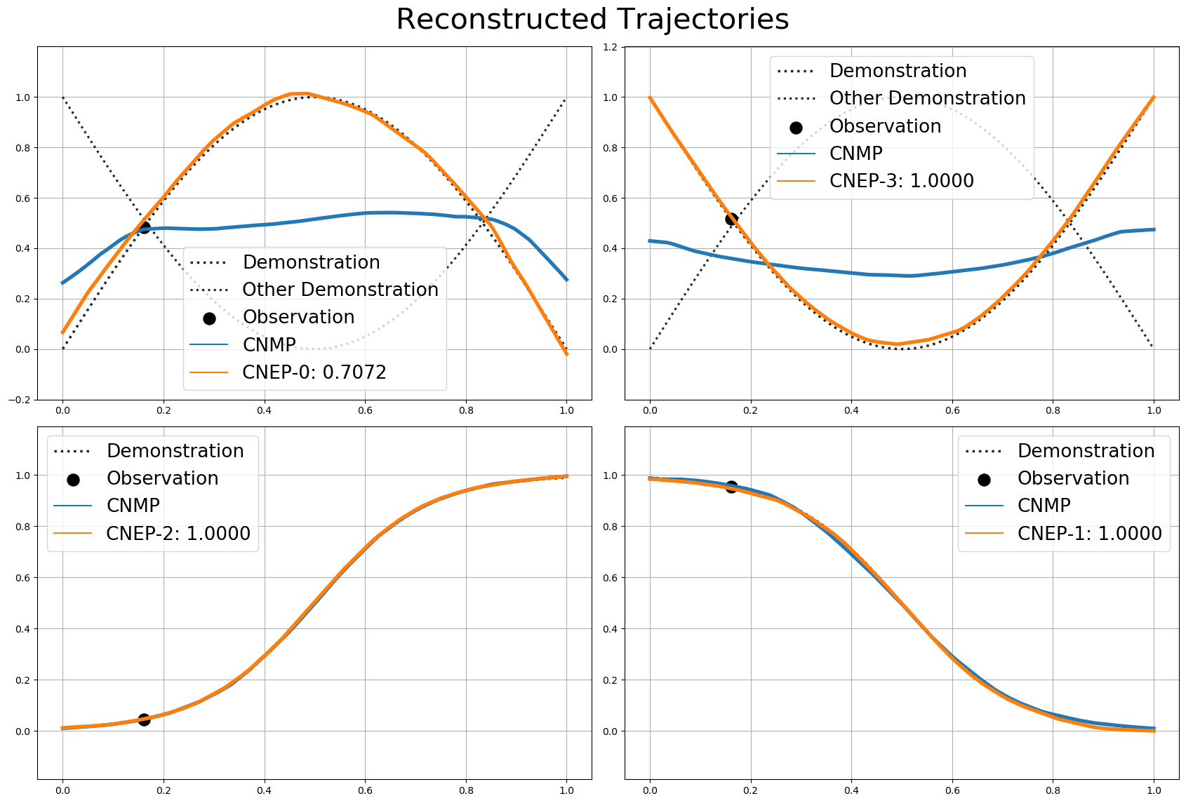
(a)

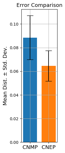
(b)

Figure 6: In (a), generated trajectories with CNEP and CNMP models are plotted for an example run. As expected, an average response is produced by the CNMP (shown in blue) when conditioned on the intersection point of multiple candidate trajectories. Yet, CNEP (shown in orange) picks one of the candidate modes. In (b), mean trajectory generation errors are illustrated. These errors are computed over 30 different runs. In each run, both models are trained from scratch and tested using observation points shown in Fig. 5b. The results are found to be statistically significant.

The above examples show how models behave over exemplary cases. When all the points in Fig. 5b are used, it can be seen in Fig. 6b that fewer errors are produced by CNEP.

IV-C Interpolation performance in the real world

In this section, we evaluate the performance of our system when it is required to interpolate, in other words, when it is conditioned from the novel points. In this evaluation, a robotic manipulator, the Baxter robotic platform, is used [28]. Two demonstrations of a pick-and-place task are collected following the kinesthetic teaching approach [3]. Demonstrations of seven distinct joints of the manipulator in the joint space and the precise 7D position of the end effector in the Cartesian space are recorded as SM trajectories. The robotic platform and the environment used in this experiment are shown in Fig. 7.

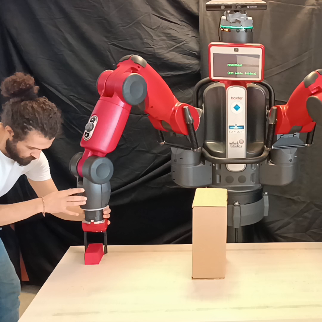
(a)

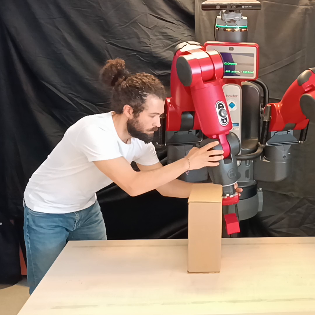
(b)

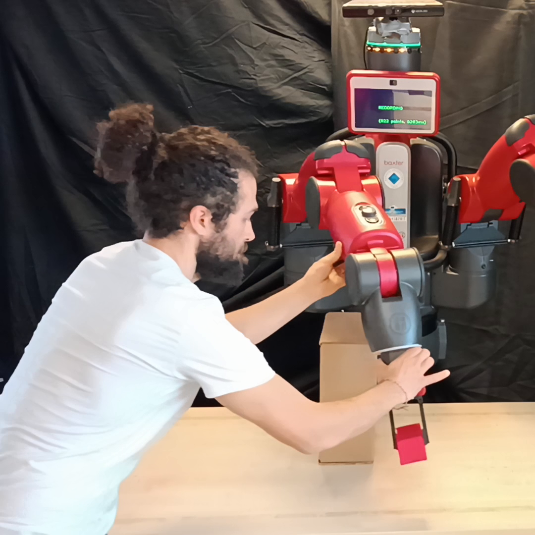
(c)

Figure 7: Pick-and-place demonstrations are performed by an expert. Kinesthetic teaching is used to generate sensorimotor demonstrations. Later, this data is used to train CNEP and CNMP models.

The dataset from these demonstrations comprises two SM trajectories that move the robot arm from a start position to an end position while avoiding an obstacle: a U-shaped curve and its mirrored counterpart, effectively forming a reverse U-shaped trajectory. We carried out two comparisons; for the first one, we trained both models on the data collected in the Cartesian space, and for the second one, we used the data collected in the joint space. To delve deeper into the capabilities of our models, we chose to condition both the CNMP and CNEP on distinctive starting points. These conditioning points were selected to lie at the midpoint between the initiation points of the two demonstrations to show the generalization capabilities of models.

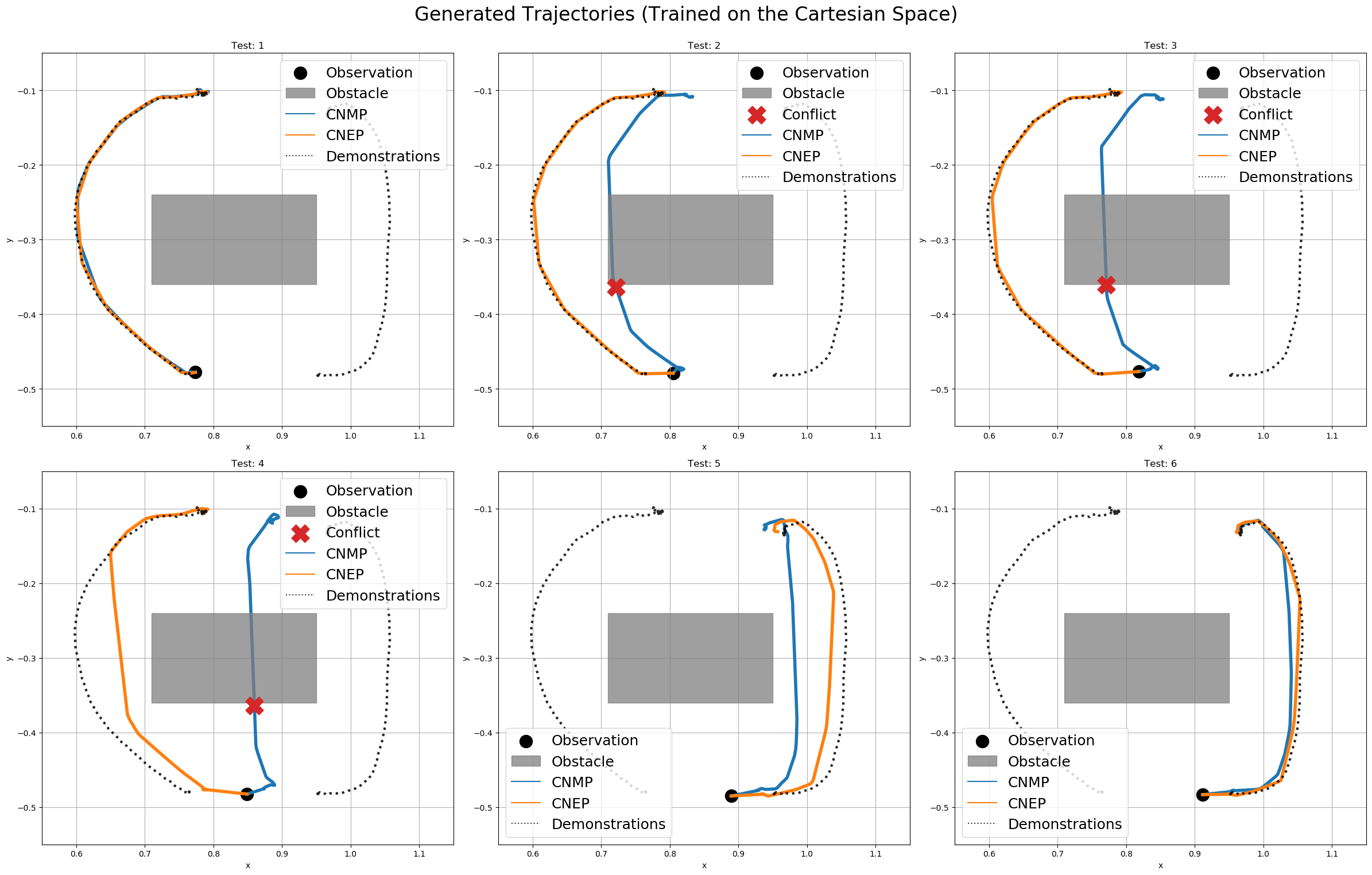
(a) Trajectory generation in the Cartesian space.

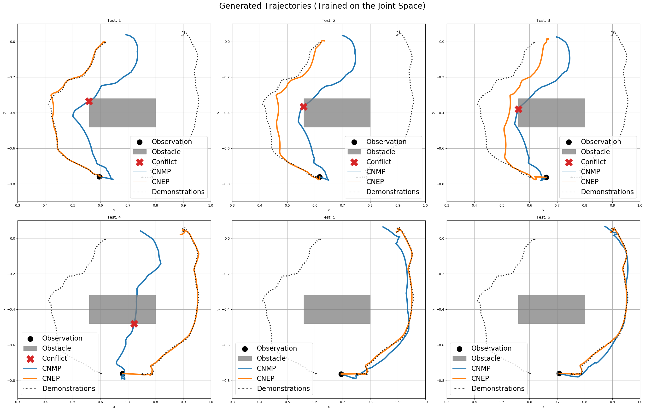
(b) Trajectory generation in the joint space.

Figure 8: Two comparisons are made using the expert demonstrations (shown with dashed lines). In (a), the coordinates of the end effector in the Cartesian Space are used to train both models. In (b), joint angles of the 7DoF manipulator are used. Conditioned on an observation (shown with $\bullet$), CNEP (shown in orange) chooses one of the modes and generates motion trajectories closer to the demonstrations. On the other hand, CNMP (shown in blue) interpolates between suitable modes, leading to collisions (shown with X) with the obstacle (shown in gray).

After training, both models were asked to realize the obstacle avoidance skill. In the first case, where models were trained with the trajectories of end-effector positions, generated values are passed through a PID controller and an inverse kinematics module before the execution on the robot. Similarly, generated joint angle values are passed through a PID controller and a forward kinematics module in the second case for illustration purposes. Results in Fig. 8 indicate a distinctive pattern, supporting our initial claim. While the CNMP tends to interpolate between the provided demonstrations, the CNEP demonstrates a preference for adhering closely to the demonstrated behaviors. To explain the implications of this behavior for real-world robot tasks, we run the trained models on the real robot and present the results in Fig. 9. Given these demonstrations, CNMP-generated trajectories lead to collisions while CNEP-generated trajectories can safely avoid obstacles.

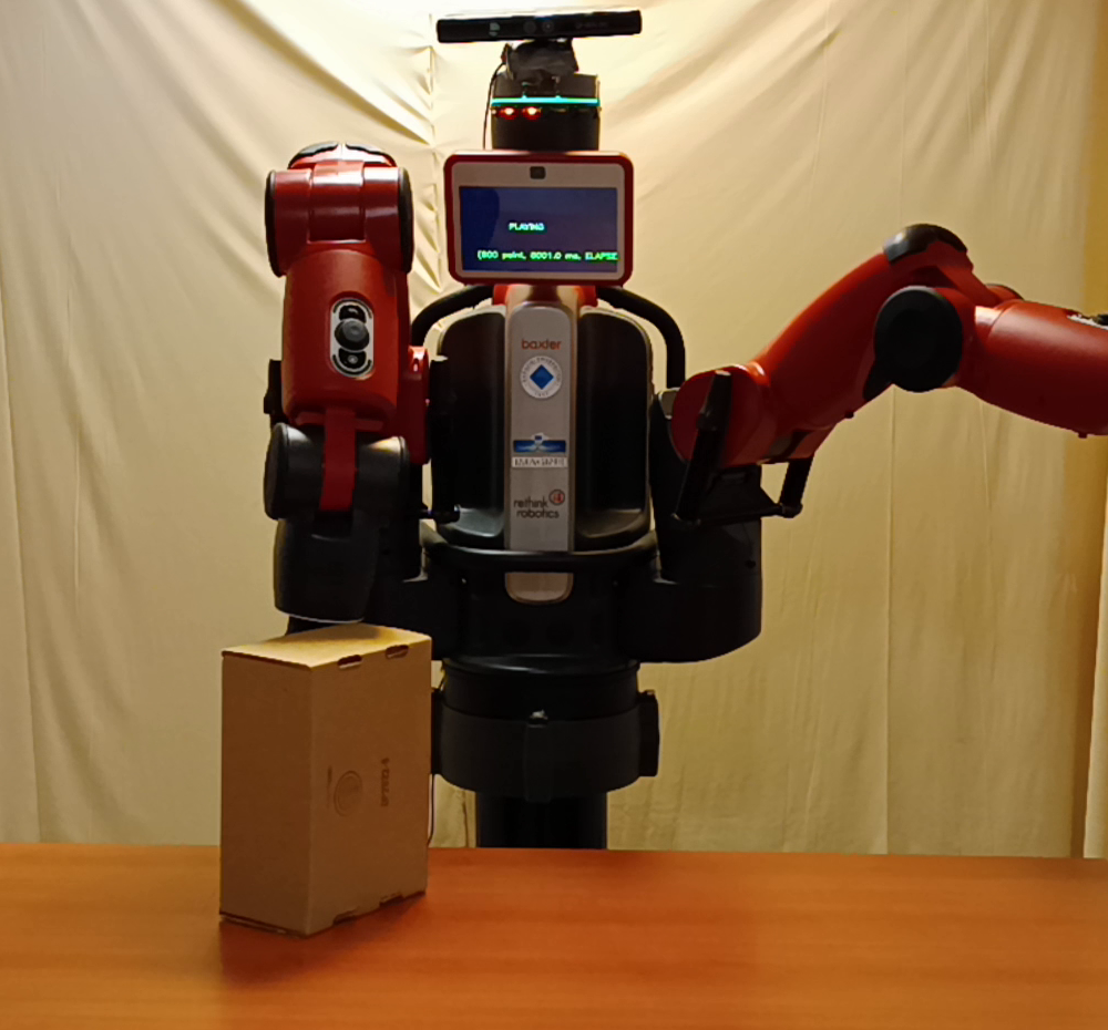
(a)

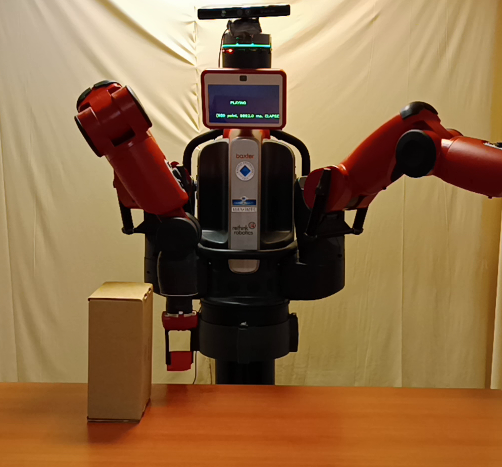
(b)

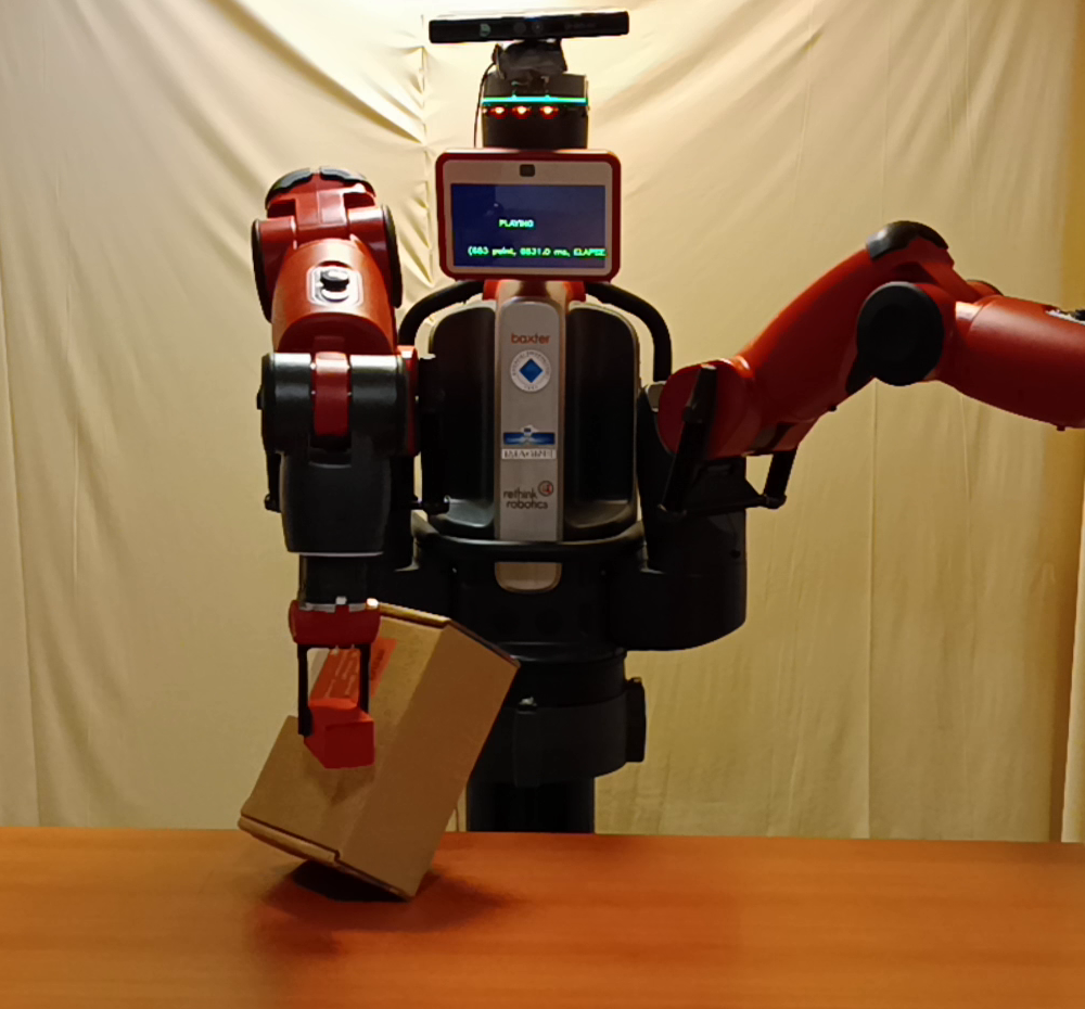
(c)

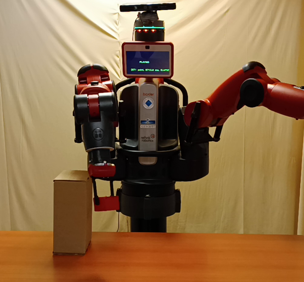
(d)

Figure 9: In (a) and (c), the generated trajectories by the CNMP model collide with the box in the middle. In (b) and (d), CNEP only interpolates within demonstrations from one mode and, therefore, follows one of the possible modes, successfully generating paths that avoid obstacles.

V Conclusion

In this study, we introduced an LfD method, namely the Conditional Neural Expert Processes. CNEP is designed to improve the modeling and generation capabilities of LfD systems when available demonstrations correspond to diverse, multimodal sensorimotor trajectories. This is achieved by the utilization of: (1) the novel architectural components, the Gate Network and the experts, and (2) the novel components of the loss function, the batch entropy and the individual entropy.

Our experiments demonstrated that CNEP can learn from motions that include significantly different trajectories; it can generate the required trajectories even when it is conditioned from the intersection points of the learned trajectories, and it can interpolate well when conditioned from novel points in the demonstration space. We showed its superior performance over the baseline CNMP model and its effectiveness in real robot experiments. The number of experts is set manually in this work and can be optimized as a hyperparameter in the future.

References

- [1] A. Segre and G. DeJong, “Explanation-based manipulator learning: Acquisition of planning ability through observation,” in Proceedings. 1985 IEEE International Conference on Robotics and Automation, vol. 2. IEEE, 1985, pp. 555–560.
- [2] H. Ravichandar, A. S. Polydoros, S. Chernova, and A. Billard, “Recent advances in robot learning from demonstration,” Annual review of control, robotics, and autonomous systems, vol. 3, pp. 297–330, 2020.
- [3] B. D. Argall, S. Chernova, M. Veloso, and B. Browning, “A survey of robot learning from demonstration,” Robotics and autonomous systems, vol. 57, no. 5, pp. 469–483, 2009.
- [4] O. Kroemer, S. Niekum, and G. Konidaris, “A review of robot learning for manipulation: Challenges, representations, and algorithms,” The Journal of Machine Learning Research, vol. 22, no. 1, pp. 1395–1476, 2021.
- [5] S. Schaal, J. Peters, J. Nakanishi, and A. Ijspeert, “Learning movement primitives,” in Robotics Research. The Eleventh International Symposium: With 303 Figures. Springer, 2005, pp. 561–572.
- [6] A. Paraschos, C. Daniel, J. Peters, and G. Neumann, “Using probabilistic movement primitives in robotics,” Autonomous Robots, vol. 42, pp. 529–551, 2018.
- [7] M. Garnelo, D. Rosenbaum, C. Maddison, T. Ramalho, D. Saxton, M. Shanahan, Y. W. Teh, D. Rezende, and S. A. Eslami, “Conditional neural processes,” in International conference on machine learning. PMLR, 2018, pp. 1704–1713.
- [8] M. Y. Seker, M. Imre, J. H. Piater, and E. Ugur, “Conditional neural movement primitives.” in Robotics: Science and Systems, vol. 10, 2019.
- [9] E. Pignat and S. Calinon, “Bayesian gaussian mixture model for robotic policy imitation,” IEEE Robotics and Automation Letters, vol. 4, no. 4, pp. 4452–4458, 2019.
- [10] J. Canny, A. Rege, and J. Reif, “An exact algorithm for kinodynamic planning in the plane,” in Proceedings of the sixth annual symposium on Computational geometry, 1990, pp. 271–280.
- [11] M. Saveriano, F. J. Abu-Dakka, A. Kramberger, and L. Peternel, “Dynamic movement primitives in robotics: A tutorial survey,” The International Journal of Robotics Research, vol. 42, no. 13, pp. 1133–1184, 2023.
- [12] M. J. Zeestraten, I. Havoutis, J. Silvério, S. Calinon, and D. G. Caldwell, “An approach for imitation learning on riemannian manifolds,” IEEE Robotics and Automation Letters, vol. 2, no. 3, pp. 1240–1247, 2017.
- [13] A. B. Pehlivan and E. Oztop, “Dynamic movement primitives for human movement recognition,” in IECON 2015-41st Annual Conference of the IEEE Industrial Electronics Society. IEEE, 2015, pp. 002 178–002 183.
- [14] H. Girgin and E. Ugur, “Associative skill memory models,” in 2018 IEEE/RSJ International Conference on Intelligent Robots and Systems (IROS). IEEE, 2018, pp. 6043–6048.
- [15] S. Calinon, “A tutorial on task-parameterized movement learning and retrieval,” Intelligent service robotics, vol. 9, pp. 1–29, 2016.
- [16] E. Ugur and H. Girgin, “Compliant parametric dynamic movement primitives,” Robotica, vol. 38, no. 3, pp. 457–474, 2020.
- [17] D. Nguyen-Tuong, M. Seeger, and J. Peters, “Model learning with local gaussian process regression,” Advanced Robotics, vol. 23, no. 15, pp. 2015–2034, 2009.
- [18] M. P. Deisenroth, D. Fox, and C. E. Rasmussen, “Gaussian processes for data-efficient learning in robotics and control,” IEEE transactions on pattern analysis and machine intelligence, vol. 37, no. 2, pp. 408–423, 2013.
- [19] M. Arduengo, A. Colomé, J. Lobo-Prat, L. Sentis, and C. Torras, “Gaussian-process-based robot learning from demonstration,” Journal of Ambient Intelligence and Humanized Computing, pp. 1–14, 2023.
- [20] A. Paraschos, C. Daniel, J. R. Peters, and G. Neumann, “Probabilistic movement primitives,” Advances in neural information processing systems, vol. 26, 2013.
- [21] A. Alahi, K. Goel, V. Ramanathan, A. Robicquet, L. Fei-Fei, and S. Savarese, “Social lstm: Human trajectory prediction in crowded spaces,” in Proceedings of the IEEE conference on computer vision and pattern recognition, 2016, pp. 961–971.
- [22] M. Pekmezci, E. Ugur, and E. Oztop, “Learning system dynamics via deep recurrent and conditional neural systems,” in 2021 29th Signal Processing and Communications Applications Conference (SIU). IEEE, 2021, pp. 1–4.
- [23] Y. Yildirim and E. Ugur, “Learning social navigation from demonstrations with conditional neural processes,” Interaction Studies, vol. 23, no. 3, pp. 427–468, 2022.
- [24] S. E. Ada and E. Ugur, “Meta-world conditional neural processes,” arXiv preprint arXiv:2302.10320, 2023.
- [25] A. Gasparetto and V. Zanotto, “A new method for smooth trajectory planning of robot manipulators,” Mechanism and machine theory, vol. 42, no. 4, pp. 455–471, 2007.
- [26] L. Biagiotti and C. Melchiorri, Trajectory planning for automatic machines and robots. Springer Science & Business Media, 2008.
- [27] L. Biewald et al., “Experiment tracking with weights and biases,” Software available from wandb.com, vol. 2, p. 233, 2020.
- [28] S. Cremer, L. Mastromoro, and D. O. Popa, “On the performance of the baxter research robot,” in 2016 IEEE international symposium on assembly and manufacturing (ISAM). IEEE, 2016, pp. 106–111.