Interacting Particle Systems on Networks:
joint inference of the network and the interaction kernel

Abstract

Modeling multi-agent systems on networks is a fundamental challenge in a wide variety of disciplines. We jointly infer the weight matrix of the network and the interaction kernel, which determine respectively which agents interact with which others, and the rules of such interactions, from data consisting of multiple trajectories. The estimator we propose leads naturally to a non-convex optimization problem, and we investigate two approaches for its solution: one is based on the alternating least squares (ALS) algorithm; another is based on a new algorithm named operator regression with alternating least squares (ORALS). Both algorithms are scalable to large ensembles of data trajectories. We establish coercivity conditions guaranteeing identifiability and well-posedness. The ALS algorithm appears statistically efficient and robust even in the small data regime, but lacks performance and convergence guarantees. The ORALS estimator is consistent and asymptotically normal under a coercivity condition. We conduct several numerical experiments ranging from Kuramoto particle systems on networks to opinion dynamics in leader-follower models.

Keywords: interacting particle systems; agent-based models; graph learning; alternating least squares; data-driven modeling

Mathematics Subject Classification: 62F12, 82C22

1 Introduction

Interaction topology plays an important role in the dynamics of many multi-agent systems, such as opinions on social networks, flows on electric power grids or airport networks, or the abstract space meshes in numerical computations [BLM⁺06, TJP03, OSFM07, PM21, WPC⁺20]. Therefore, it is of paramount interest to learn such systems from data.

We consider a heterogeneous dynamical system with $N$ interacting agents on a graph: let $G=(V,E,\mathbf{a})$ be a graph with weight matrix $\mathbf{a}=(\mathbf{a}_{ij})\in[0,1]^{N\times N}$ and $\mathbf{a}_{ij}>0$ iff $(i,j)\in E$, and at each vertex $i\in[N]:=\{1,\dots,N\}$ there is an agent with a state represented, at time $t$, by a vector $X_{t}^{i}\in\mathbb{R}^{d}$. Suppose that the evolution of the state $(X_{t}^{i})_{i\in[N]}\in\mathbb{R}^{N\times d}$ of the system at time $t$ is governed by the system of ODEs/SDEs:

$$\mathcal{S}_{{\mathbf{a}},{\Phi}}\,:\qquad d{X}^{i}_{t}=\sum_{j\neq i}\mathbf{a}_{ij}\Phi(X^{j}_{t}-X^{i}_{t})dt+\sigma d{W}^{i}_{t},\quad i=1,\ldots,N\,,$$ (1.1)

where we write $\sum_{j\neq i}$ to denote $\sum_{j\in[N]\setminus\{i\}}$. The interaction kernel $\Phi:\mathbb{R}^{d}\rightarrow\mathbb{R}^{d}$ determines the interaction laws, which, crucially, apply only when $\mathbf{a}_{ij}$ is strictly positive. The random initial condition $(X_{t_{0}}^{i})_{i\in[N]}$ is sampled from a probability measure $\mu$ on $\mathbb{R}^{N\times d}$. The forcing term $(W^{i}_{t})_{i\in V}$ is an $\mathbb{R}^{N\times d}$-valued standard Brownian motion. The diffusion coefficient $\sigma$ is a constant; the system is deterministic when $\sigma=0$ and stochastic when $\sigma>0$. Various normalizations of the weight matrix exist. For example, one may consider an unweighted graph $G=(V,E,A)$ with a binary matrix with $a_{ij}\in\{0,1\}$ denoting the connection or disconnection between node $i$ and node $j$; one may also consider a normalization by letting $\mathbf{a}_{ij}=\frac{1}{|\mathcal{N}_{i}|}a_{ij}$, where the set $\mathcal{N}_{i}=\{j\in V:(j,i)\in E,j\neq i\}$ is the directed neighborhood of vertex $i$ in the graph $G$, consisting of those vertices that can influence $i$ when $a_{ij}=1$. These normalizations become important when one studies the mean-field limit $N\rightarrow+\infty$, see, e.g., [LRW23] and references therein. In this study, we will normalize the rows of $\mathbf{a}$ in $\ell^{2}$, but both theory and algorithms are unaffected by this choice and apply to other normalizations.

We study the following statistical inference problem: given knowledge of the general form of System (1.1) and multi-trajectory data of the system, jointly estimate the unknown weight matrix $\mathbf{a}$ and the interaction kernel $\Phi$.

This joint estimation is a nonlinear inverse problem, since the data depends on the product of the two unknowns $\mathbf{a}$ and $\Phi$ in (1.1). The two unknowns play significantly different roles in the dynamics: $\mathbf{a}$ encodes the geometry of the space on which the agents are allowed to interact and has no structure nor symmetries; meanwhile, $\Phi$ is the law for all interactions, which is a common structure that will enable to tackle the task without requiring an excessive number of observations.

When the graph is complete and undirected, i.e., $\mathbf{a}_{ij}\equiv\frac{1}{N}$ for all $(i,j)$, we have homogeneous interactions. In this case, the learning of radial interaction kernels $\Phi$ in the form $\Phi(x,y)=\phi(|x-y|)\frac{x-y}{|x-y|}$ has been systematically studied in [LZTM19, LMT21a, LMT21b, LLM⁺21] and generalized to second-order systems and non-radial interaction kernels [MTZM23], and even to interaction kernels whose variables are learned [FMMZ22]. Generally, when the graph is directed and incomplete with a general weight matrix, we have heterogeneous interactions. These graphs arise in various applications, for example, when the agents’ interactions are constrained (e.g., on a fixed communication/social network), or when agents have different influence power (e.g., leaders/followers in a social network, websites, airport hubs with low/high connectivity, etc…). The learning of the interaction kernel from a single trajectory, assuming knowledge of the underlying network, has been studied in [ASM22]. Another related problem is estimating the graph underlying linear Markovian dynamics on the graph when only sparse observations in space and time are given [CK22]. However, none of these works address the joint estimation problem.

1.1 Problem setup

We assume that the weight matrix $\mathbf{a}$ is in the admissible set

$$\mathcal{M}:=\bigg{\{}\mathbf{a}=(\mathbf{a}_{ij})\in[0,1]^{N\times N}\!:\,\forall i\in[N]\,\,\,\mathbf{a}_{ii}=0\,\,,\,\,|\mathbf{a}_{i\cdot}|^{2}:=\|\mathbf{a}_{i\cdot}\|_{\ell^{2}}^{2}=\sum_{j=1}^{N}\mathbf{a}_{ij}^{2}=1\,\bigg{\}}\,.$$ (1.2)

This removes a trivial issue in the identifiability of $(\mathbf{a},\Phi)$ due to rescaling: $(\mathbf{a},\Phi)$ can be replaced by $(\lambda\mathbf{a},\lambda^{-1}\Phi)$ in (1.1), for any $\lambda>0$, without changing the trajectories, and therefore the observations. The choice of the $\ell^{2}$ normalization is not essential in our analysis and algorithms; other norms, such as the $\ell^{1}$-norm or the Frobenius norm, may be used depending on the modeling assumptions.

Table 1: Notations for the indices, vectors, and arrays in the system.

$[N]$ : index set $\{1,\dots,N\}$	$\mathbf{X}_{t}=(X^{1}_{t},\ldots,X^{N}_{t})\in\mathbb{R}^{N\times d}$: state vector at time $t$
$i,j\in[N]$: index for agents	$\mathbf{a}\in\mathbb{R}^{N\times N}$: graph weight matrix
$k\in[p]$: index for basis of kernel	$c\in\mathbb{R}^{p\times 1}$: coefficient vector of $K$ on a basis $\{\psi_{k}\}$
$m\in[M]$: index for samples	$\mathbf{B}(\mathbf{X}_{t})=\big{(}\psi_{k}(X_{t}^{j}-X_{t}^{i})\big{)}_{j,i,k}\in\mathbb{R}^{N\times N\times d\times p}$: basis array
$l\in[L]$: index of time instants	$\|\cdot\|_{F}$: the Frobenius norm of a matrix
$|\cdot|$: the Euclidean norm of a vector	${\rm{Vec}}:\mathbb{R}^{N\times p}\to\mathbb{R}^{Np\times 1}$ is the vectorization operation.

* We use letters for vectors, bold letters for arrays/matrices of dimension dependent on $N$, and calligraphic letters for operators.

In this work, we restrict our attention to parametric families of interaction kernels: we estimate the coefficient $c=(c_{1},\ldots,c_{p})\in\mathbb{R}^{p}$ of the kernel $\Phi(x)=\sum_{k=1}^{p}c_{k}\psi_{k}(x)$ under a given set of basis functions $\{\psi_{k}\}_{k=1}^{p}$. However, we don’t require the true interaction kernel to be in the hypothesis space $\mathcal{H}:=\mathrm{span}\{\psi_{k}\}_{k=1}^{p}$, and our estimator is robust to mis-specification of basis functions with regularization.

We let $\mathbf{X}_{t}:=(X^{1}_{t},\ldots,X^{N}_{t})\in\mathbb{R}^{N\times d}$ be the state vector, $\dot{\mathbf{W}}:=[dW^{i}_{t}]_{i}\in\mathbb{R}^{N\times d}$ be the white noise in the forcing term, and $\mathbf{B}(\mathbf{X}_{t})_{i}:=\big{(}\psi_{k}(X_{t}^{j}-X_{t}^{i})\big{)}_{j,k}\in\mathbb{R}^{N\times 1\times d\times p}$ for each $i\in[N]$. We can then rewrite (1.1) in tensor form:

$$\mathcal{S}_{{\mathbf{a}},{c}}\quad: \dot{\mathbf{X}}_{t}=\mathbf{a}\mathbf{B}(\mathbf{X}_{t})c+\sigma\dot{\mathbf{W}}=\big{(}\mathbf{a}_{i\cdot}\mathbf{B}(\mathbf{X}_{t})_{i}c\big{)}_{i\in[N]}+\sigma\dot{\mathbf{W}}\,,\quad\text{ where}$$ (1.3)

$$\mathbf{a}_{i\cdot}\mathbf{B}(\mathbf{X}_{t})_{i}c=\sum_{j\neq i}\mathbf{a}_{ij}\sum_{k=1}^{p}\psi_{k}(X^{j}_{t}-X^{i}_{t})c_{k}\in\mathbb{R}^{d}\,,\quad i\in[N],$$

with $\mathbf{a}_{i\cdot}$ is the $i$-th row of the matrix $\mathbf{a}$. We summarize the notation in Table 1.

Problem statement.

Our goal is to jointly estimate the weight matrix $\mathbf{a}$ and the coefficient vector $c$, and therefore the interaction kernel $\Phi$, given

$$\vspace{-1mm}\smash{\textbf{Data: }\quad\{\mathbf{X}_{t_{0}:t_{L}}^{m}\}_{m=1}^{M},\quad\text{ where }t_{0}:t_{L}\text{ denotes }(t_{0},t_{1},t_{2},\ldots,t_{L})\,,\text{ with }t_{l}=l\Delta t\,,}$$ (1.4)

i.e., observations of the state vector at discrete times along multiple-trajectories indexed by $m$, started from initial conditions $\mathbf{X}^{m}_{t_{0}}$ sampled from $\mu^{\otimes N}$, where $\mu$ is a distribution on $\mathbb{R}^{d}$. We let $T=t_{L}$ and $t_{0}=0$.

1.2 Proposed estimator: scalable algorithms, identifiability, and convergence

Our estimator of the parameter $(\mathbf{a},c)$ is a minimizer of a loss function $\mathcal{E}_{L,M}$:

$$(\widehat{\mathbf{a}},\widehat{c})=\underset{(\mathbf{a},c)\in\mathcal{M}\times\mathbb{R}^{p}}{\operatorname{arg}\operatorname{min}}\;\mathcal{E}_{L,M}(\mathbf{a},c),\,\,\,\text{ with }\quad\mathcal{E}_{L,M}(\mathbf{a},c):=\frac{1}{MT}\sum_{l=0,m=1}^{L-1,M}\left\|\Delta\mathbf{X}_{t_{l}}^{m}-\mathbf{a}\mathbf{B}(\mathbf{X}_{t_{l}}^{m})c\Delta t\right\|_{F}^{2},$$ (1.5)

where $\mathcal{M}$ is the admissible set defined in (1.2) and $\|\cdot\|_{F}$ denotes the Frobenuous norm on $\mathbb{R}^{N\times d}$. Here $\Delta\mathbf{X}_{t_{l}}=\mathbf{X}_{t_{l+1}}-\mathbf{X}_{t_{l}}$; if the system were deterministic ($\sigma=0$) and we had observations of $\dot{\mathbf{X}}_{t_{l}}$, we use these instead. This loss function comes from the differential system (1.3): its scaled version $(\Delta t)^{-1}\mathcal{E}_{L,M}(\mathbf{a},c)$ is the mean square error between the two sides of the system when $\sigma=0$; it is the scaled log-likelihood ratio (up to a constant independent of the data trajectories) for the stochastic system when $\sigma>0$.

The loss function $\mathcal{E}_{L,M}$ is non-convex in $(\mathbf{a},c)$, but quadratic in either $\mathbf{a}$ or $c$ separately; the optimization landscape may have multiple local minima. This joint estimation problem is closely related to compressed sensing and matrix sensing as elaborated in seminal works including [Can08, CR09, CT10, RFP10, GJZ17, ZSL19]. The array $\{\mathbf{B}(\mathbf{X}_{t_{l}}^{m})\}$ plays the role of sensing linear operator for the unknowns $\mathbf{a}$ and $c$. Diverging from the conventional framework of matrix sensing, where the entries of the sensing matrix are typically independent, the entries of $\mathbf{B}(\mathbf{X}_{t_{l}}^{m})$ are correlated, depending on the dynamics and the basis functions. Furthermore, here we have the additional constraint that the entries of the weight matrix $\mathbf{a}$ are nonnegative. These differences can lead to multiple local minima for the loss function $\mathcal{E}_{L,M}$, even in the limit $M\rightarrow\infty$, posing a risk for methods such as deterministic gradient descent.

We introduce coercivity conditions in Section 2.2.1, key properties in the learning theory of interaction kernels (see, for example, [LMT21a, LMT21b, LLM⁺21]) that guarantee the identifiability of the parameters and the well-posedness of the inverse problem. The coercivity conditions are closely related to the Restricted Isometry Property (RIP) conditions in matrix sensing.

We consider two efficient algorithms for computing the estimator. The first one is based on classical alternating minimization over $\mathbf{a}$ and $c$, and since such minimization steps lead to least squares problems, this corresponds to Alternating Least Squares (ALS) [KDL80]. The second one, called ORALS, is based on first an Operator Regression, which estimates product matrices of $\mathbf{a}$ and $c$, and then uses ALS on much simpler matrix factorization problems to obtain the factors $\mathbf{a}$ and $c$ from the estimated products.

The number of parameters $(\mathbf{a},c)$ to be estimated is $N^{2}+p$, and the number of scalar observations is $MLNd$. Ideally, an estimator will perform well when $MLNd\gtrsim N^{2}+p$. This is, however, quite optimistic in general, as we have independence of the observations in $M$, but not in $L$ or $N$ or $d$; the dependency in $L$ is dependent on the dynamics of the system, as more observations on a longer interval of time may not add information useful to the estimation, for example, depending on whether the system is ergodic or not. Thus, a more realistic expectation for the minimal sample requirements is $M\approx N^{2}+p$, which we call the critical sampling regime. The estimator constructed by ALS shows nearly ideal estimation performance in this critical sample size regime, but it lacks a theoretical justification for such performance, and even for its convergence. ORALS appears to perform comparably well only in the large sample regime $M\gtrsim N^{2}p$, but we are able to analyze its performance as $M\rightarrow\infty$, proving convergence and even asymptotic normality.

1.3 Extensions

General pairwise interaction kernels. Our estimators and algorithms are immediately applicable to general interaction kernels in the form $\Phi(X^{j},X^{i})$ (or on a variety of variables, as in the Euclidean settings considered in [MTZM23]), since the estimation is parametric. The theoretical analysis can also be generalized in this direction by suitably modifying the coercivity conditions that are crucial in proving the estimator’s uniqueness and well-posedness.

Nonparametric estimation. In this study, we consider the parametric estimation, where $\Phi$ is approximated on the finite-dimensional hypothesis space $\mathcal{H}=\{\psi_{k}\}_{k=1}^{p}$. For nonparametric estimation, the dimension of the hypothesis space must adaptively increase with the number of observations. Algorithmically, this is a direct extension of this work, but its analysis, particularly the optimal convergence rate, is more involved and not developed here; see [LZTM19, LMT21a, LMT21b, LLM⁺21] for the case of particles in Euclidean space.

Agents of different types. In many applications, there are different types of agents, for example, different types of cells or genetic genes in biology, prey and predators in ecological models, leaders and followers in social networks, and so on. The model we introduce above may be generalized to some of these settings, by considering a system with $Q$ types of agents and corresponding interaction kernels $(\Phi_{q})_{q=1}^{Q}$, where the type of agent $i$ is denoted by $\kappa(i)$, and governing equations

$$\mathcal{S}_{{\mathbf{a}},{(\Phi_{q})_{q=1}^{Q},\kappa}}\,:\qquad d{X}^{i}_{t}=\sum_{j\neq i}\mathbf{a}_{ij}\Phi_{\kappa(i)}(X^{j}_{t}-X^{i}_{t})dt+\sigma d{W}^{i}_{t},\quad i\in[N]\,.$$ (1.6)

We tackle here the challenging problem where the type $\kappa$ of each agent is not known, and it needs to be estimated together with the weight matrix $\mathbf{a}$ and the interaction kernels $\phi_{1},\dots,\phi_{Q}$. We introduce a three-fold ALS algorithm to solve this problem; see Section 4.3.

2 Construction and analysis of the estimator, via ALS and ORALS

We detail the two algorithms we propose for constructing the estimator in (1.5): an Alternating Least Squares (ALS) approach and a new two-step algorithm based on Operator Regression followed by an Alternating Least Squares (ORALS), present their theoretical guarantees with new coercivity conditions, and discuss their computational complexity. ALS is computationally efficient, with well-conditioned matrices as soon the number of observations is comparable to the number of unknown parameters $(\mathbf{a},c)$, but with weak theoretical guarantees. ORALS is amenable to theoretical analysis, achieving consistency and asymptotic normality, albeit at a somewhat higher (in $N$ and $p$) computational cost. We will further examine their numerical performance in the next section.

2.1 Two algorithms: ALS and ORALS

2.1.1 Alternating Least Squares (ALS)

The ALS algorithm exploits the convexity in each variable by alternating between the estimation of the weight matrix $\mathbf{a}$ and of the coefficient $c$ while keeping the other fixed:

Inference of the weight matrix. Given an interaction kernel, represented by the corresponding set of coefficients $c$, we estimate the weight matrix $\mathbf{a}$ by directly solving the minimizer of the quadratic loss function with $c$ fixed, followed by row-normalizing the estimator. For every $i\in[N]$, we obtain the minimizer (with $\mathbf{a}_{ii}=0$) of the loss function $\mathcal{E}_{L,M}(\mathbf{a},c)$ in (1.5) with $c$ fixed by solving $\nabla_{\mathbf{a}_{i\cdot}}\mathcal{E}_{L,M}(\mathbf{a},c)=0$, which is a linear equation in $\mathbf{a}_{i\cdot}$:

$$\widehat{\mathbf{a}}_{i\cdot}\mathcal{A}^{\textrm{ALS}}_{c,M,i}:=\widehat{\mathbf{a}}_{i\cdot}([\mathbf{B}(\mathbf{X}_{t_{l}}^{m})_{i}]_{l,m}c) =[(\Delta\mathbf{X}^{m}_{t_{l}})_{i}]_{l,m}/\Delta t\,,\qquad i\in[N],$$ (2.1)

where $[\mathbf{B}(\mathbf{X}_{t_{l}}^{m})_{i}]_{l,m}\in\mathbb{R}^{N\times(dLM)\times p}$, $\mathcal{A}^{\textrm{ALS}}_{c,M,i}:=[\mathbf{B}(\mathbf{X}_{t_{l}}^{m})_{i}]_{l,m}c\in\mathbb{R}^{N\times(dLM)}$ and $[\Delta\mathbf{X}_{t_{l}}^{m}]_{l,m}\in\mathbb{R}^{N\times dLMN}$ are obtained by matrix-vector multiplication of the appropriate tensor slices by $c$. We solve this linear system by least squares with nonnegative constraints [LH95, Chapter 23], since $\mathbf{a}\in\mathcal{M}$ implies that the entries of $\mathbf{a}$ are nonnegative, followed by a normalization in $\ell^{2}$-norm to obtain an estimator $\widehat{\mathbf{a}}_{i\cdot}$ in the admissible set $\mathcal{M}$ defined in (1.2).

Estimating the parametric interaction kernel. In this step, we estimate the parameter $c$ by minimizing the loss function $\mathcal{E}_{L,M}(\mathbf{a},c)$ in (1.5) with a fixed weight matrix $\mathbf{a}$ estimated above, by solving the least squares problem

$$\mathcal{A}^{\textrm{ALS}}_{\mathbf{a},M}\,\widehat{c}:=[\mathbf{a}\mathbf{B}(\mathbf{X}_{t_{l}}^{m})]_{l,m}\widehat{c}=[\Delta\mathbf{X}_{t_{l}}^{m}]_{l,m}/\Delta t\,,$$ (2.2)

where $\mathcal{A}^{\textrm{ALS}}_{\mathbf{a},M}:=[\mathbf{a}\mathbf{B}(\mathbf{X}_{t_{l}}^{m})]_{l,m}\in\mathbb{R}^{dLMN\times p}$ is again obtained by stacking in a block-row fashion and $\mathcal{A}^{\textrm{ALS}}_{\mathbf{a},M,i}:=[\mathbf{a}\mathbf{B}(\mathbf{X}_{t_{l}}^{m})_{i}]_{l,m}$.

We alternate these two steps until the updates to the estimators are smaller than a tolerance threshold $\epsilon$ or until maximal iteration number $n_{maxiter}$ is reached, as in Algorithm 1.

Algorithm 1 ALS: alternating least squares

procedure ALS_IPSonGraph($\{\mathbf{X}^{m}_{t_{0}:t_{L}}\}_{m=1}^{M},\{\psi_{k}\}_{k=1}^{p},\epsilon,{n}_{maxiter}$)

    Construct the arrays $\{\mathbf{B}(\mathbf{X}_{t_{l}}^{m})\}_{l,m}$ and $\{\Delta\mathbf{X}_{t_{l}}^{m}\}$ in (1.5) for each trajectory.

    Randomly pick an initial condition $\widehat{c}_{0}$.

    for $\tau=1,\dots,{n}_{maxiter}$ do

         Estimate the weight matrix $\widehat{\mathbf{a}}_{\tau}$ by solving (2.2) with $c=\widehat{c}_{\tau-1}$, by nonnegative least squares,  followed by a row normalization.

         Estimate the parameter $\widehat{c}_{\tau}$ by solving (2.1) with $\mathbf{a}=\widehat{\mathbf{a}}_{\tau}$, by least squares.

         Exit loop if $||\widehat{c}_{\tau}-\widehat{c}_{\tau-1}||\leq\epsilon||\widehat{c}_{\tau-1}\|$ and $||\widehat{\mathbf{a}}_{\tau}-\widehat{\mathbf{a}}_{\tau-1}||\leq\epsilon||\widehat{\mathbf{a}}_{\tau-1}||$.     return $\widehat{c}_{\tau},\widehat{\mathbf{a}}_{\tau}$.

2.1.2 Operator Regression and Alternating Least Squares (ORALS)

ORALS divides the estimation into two stages: a statistical operator regression stage and a deterministic alternating least squares stage. The first stage estimates the entries of the matrices $\{\mathbf{a}_{i,\cdot}^{\rm T}c^{\rm T}\in\mathbb{R}^{(N-1)\times p}\}_{i=1}^{N}$ (excluding the zero entries $\mathbf{a}_{ii}$) by least squares regression with regularization. It is called operator regression because we view the data as the output of a sensing operator over these matrices. After this step, a deterministic alternating least squares stage jointly factorizes these estimated matrices to obtain the weight matrix $\mathbf{a}$ and the coefficient $c$.

Operator Regression stage. Consider the arrays $\{\mathbf{Z}_{i}=\mathbf{a}_{i,\cdot}^{\rm T}c^{\rm T}\in\mathbb{R}^{(N-1)\times p}\}_{i=1}^{N}$ treated as vectors in $\mathbb{R}^{(N-1)p\times 1}$, that is, $z_{i}={\rm Vec}(\mathbf{Z}_{i})=(\mathbf{a}_{i,1}c_{1},\ldots,\mathbf{a}_{i,1}c_{p},\mathbf{a}_{i,2}c_{1},\ldots,\mathbf{a}_{i,2}c_{p},\ldots)^{\rm T}\in\mathbb{R}^{(N-1)p\times 1}$ for each $i$. They are solutions of the linear equations with sensing operators $\mathcal{A}_{i,M}=[\mathcal{A}_{i}]_{l,m}\in\mathbb{R}^{dML\times(N-1){p}}$:

$$\mathcal{A}_{i,M}z_{i}=[\mathcal{A}_{i}]_{l,m}z_{i}:=[(\mathbf{a}\mathbf{B}(\mathbf{X}_{t_{l}}^{m})c\Delta t)_{i}]_{l,m}=[(\Delta\mathbf{X}^{m}_{t_{l}})_{i}]_{l,m}\,,\quad i\in[N],$$ (2.3)

where, as usual, $[\cdot]_{l,m}$ denotes stacking block rows. With the above notation, we can write the loss function in (1.5) as

$$(\widehat{z}_{1,M},\ldots,\widehat{z}_{N,M})=\underset{z_{1},\ldots,z_{N}}{\operatorname{arg}\operatorname{min}}\;\mathcal{E}_{L,M}(z_{1},\ldots,z_{N}):=\frac{1}{ML}\sum_{l,m,i=1}^{L,M,N}\big{|}[(\Delta\mathbf{X}^{m})_{i}]_{l,m}-[\mathcal{A}_{i}]_{l,m}z_{i}\big{|}^{2}$$ (2.4)

and obtain $\{\widehat{z}_{i,M}\}$ by solving this least squares problem for each $i\in[N]$.

Deterministic ALS stage. The rows of $\mathbf{a}$ and the vector $c$ are estimated via a joint factorization of the matrices of the estimated vectors $\{\widehat{z}_{i,M}\}$, denoted by $\widehat{\mathbf{Z}}_{i,M}$, with a shared vector $c$:

$$(\widehat{\mathbf{a}}^{M},\widehat{c}^{M})=\underset{\mathbf{a}\in\mathcal{M},\,c\,\in\mathbb{R}^{p}}{\operatorname{arg}\operatorname{min}}\;\mathcal{E}(\mathbf{a},c):=\sum_{i=1}^{N}\left\|\widehat{\mathbf{Z}}_{i,M}-\mathbf{a}_{i,\cdot}^{\rm T}c^{\rm T}\right\|_{F}^{2},$$ (2.5)

where $\mathcal{M}$ is the admissible set in (1.2). A deterministic alternating least squares algorithm solves this problem: we first estimate each row of $\mathbf{a}$ by nonnegative least squares and then estimate $c$ using all the estimated $\mathbf{a}$ with row-normalization. We iterate them for two steps, starting from $\widehat{c}_{0}$ obtained from rank-1 singular value decomposition, as in Algorithm 2. Numerical tests show that two iteration steps are often sufficient to complete the factorization, and the result is robust for more iteration steps.

Theorem 2.7 shows that the estimator obtained by ORALS is consistent and, in fact, asymptotically normal under a suitable coercivity condition.

Algorithm 2 ORALS: Operator Regression and Alternating Least Squares.

procedure ORALS_IPSonGraph($\{\mathbf{X}^{m}_{t_{0}:t_{L}}\}_{m=1}^{M},\{\psi_{k}\}_{k=1}^{p}$)

    Construct the sensing operators $\mathcal{A}_{i,M}$ (from the arrays $\{\mathbf{B}(\mathbf{X}_{t_{l}}^{m})\}_{l,m}$) and $\{\Delta\mathbf{X}_{t_{l}}^{m}\}$ in (2.3) for each trajectory.

    Solve the vector $\widehat{z}_{i,M}$’s in (2.4) by least squares with regularization; and transform them into matrices $\widehat{Z}_{i,M}$.

    Factorize each matrix $\widehat{Z}_{i,M}$. Set the initial condition $\widehat{c}_{0}$ to be the first right singular vector.

    for $\tau=1,2$ do

         Estimate the weight matrix $\widehat{\mathbf{a}}_{\tau}$ by solving (2.5) with $c=\widehat{c}_{\tau-1}$ by nonnegative least squares,  followed by a row normalization.

         Estimate the parameter $\widehat{c}_{\tau}$ by solving (2.5) with $\mathbf{a}=\widehat{\mathbf{a}}_{\tau}$ by least squares.     return $\widehat{c}_{\tau},\widehat{\mathbf{a}}_{\tau}$.

2.2 Theoretical guarantees

Three fundamental issues in our inference problem are (i) the identifiability of the weight matrix and the interaction kernel, i.e., the uniqueness of the minimizer of the loss function; (ii) the well-posedness of the inverse problem in terms of the condition numbers of the regression matrices in the ALS and ORALS algorithms, and (iii) the convergence of the estimators as the sample size increases. We address these issues by introducing coercivity conditions in the next section.

Here, we say the true parameter $(\mathbf{a}^{*},\Phi_{*})$ is identifiable if it is the unique zero of the loss function in the large sample limit

$$\mathcal{E}_{L,\infty}(\mathbf{a},\phi) =\frac{1}{L}\sum_{i=1}^{N}\sum_{l=0}^{L-1}\mathbb{E}\bigg{[}\bigg{|}\sum_{j\neq i}[\mathbf{a}_{ij}\Phi(\mathbf{r}_{ij}(t_{l}))-\mathbf{a}_{ij}^{*}\Phi_{*}(\mathbf{r}_{ij}(t_{l}))]\bigg{|}^{2}\bigg{]}\,,$$

when the data has no noise and when the model is deterministic. We say the inverse problem is well-posed if the estimator is robust to noise.

2.2.1 Exploration measure

We define a function space $L^{2}(\rho_{L})$ for learning the interaction kernel, where $\rho_{L}$ is a probability measure that quantifies data exploration to the interaction kernel. Let

$$\mathbf{r}_{ij}(t_{l}):=X^{j}_{t_{l}}-X^{i}_{t_{l}}\quad\text{and}\quad\mathbf{r}_{ij}^{m}(t_{l}):=X^{j,m}_{t_{l}}-X^{i,m}_{t_{l}}\,.$$ (2.6)

These pairwise differences $\{\mathbf{r}_{ij}^{m}(t_{l})\}$ are the independent variable of the interaction kernel. Thus, we define $\rho_{L}$ as follows.

Definition 2.1 (Exploration measure)

With observations of $M$ trajectories at the discrete times $\{t_{l}\}_{l=0}^{L-1}$, we introduce an empirical measure, and its large sample limit, on $\mathbb{R}^{d}$, defined as

$$\rho_{L,M}(d\mathbf{r}) :=\frac{1}{(N-1)NLM}\sum_{l=0}^{L-1}\sum_{m=1}^{M}\sum_{1\leq i\neq j\leq N}\delta_{\mathbf{r}_{ij}^{m}(t_{l})}(d\mathbf{r}),$$ (2.7)

$$\rho_{L}(d\mathbf{r}) :=\frac{1}{(N-1)NL}\sum_{l=0}^{L-1}\sum_{1\leq i\neq j\leq{N}}\mathbb{E}[\delta_{\mathbf{r}_{ij}(t_{l})}(d\mathbf{r})]\,,$$ (2.8)

where $\sum_{1\leq i\neq j\leq{N}}$ stands for $\sum_{i=1}^{N}\sum_{j=1,j\neq i}^{N}$.

The empirical measure depends on the sample trajectories, but $\rho_{L}$ is the large sample limit, uniquely determined by the distribution of the stochastic process $\mathbf{X}_{t_{0}:t_{L-1}}$, and hence data-independent.

2.2.2 Two coercivity conditions

We introduce two types of coercivity conditions to ensure the identifiability and the invertibility of the regression matrices in ALS and ORALS. The first one is a joint type, including two coercivity conditions. We call them rank-1 and rank-2 joint coercivity conditions, which guarantee that the bilinear forms defined by the loss function in terms of either the kernel or the weight matrix are coercive (recall that a bilinear function $f(x,y)$ is coercive in a Hilbert space $\mathcal{H}$ if $f(x,x)\geq c\|x\|_{\mathcal{H}}^{2}$ for any $x\in\mathcal{H}$ [Lax02]).

Definition 2.2 (Joint coercivity conditions)

The system (1.1) is said to satisfy a rank-1 joint coercivity condition on a hypothesis function space $\mathcal{H}\subset L^{2}(\rho_{L})$ with constant $c_{\mathcal{H}}>0$ if for all $\Phi\in\mathcal{H}$ and all $\mathbf{a}\in\mathcal{M}$,

$$\frac{1}{L}\sum_{l=0}^{L-1}\mathbb{E}\bigg{[}\bigg{|}\sum_{j\neq i}\mathbf{a}_{ij}\Phi(\mathbf{r}_{ij}(t_{l}))\bigg{|}^{2}\bigg{]}\ \geq c_{\mathcal{H}}|\mathbf{a}_{i\cdot}|^{2}\|\Phi\|_{\rho_{L}}^{2}\,,\quad\forall\leavevmode\nobreak\ i\in[N]\,.$$ (2.9)

Moreover, we say system (1.1) satisfies a rank-2 joint coercivity condition on $\mathcal{H}$ if there exists a constant $c_{\mathcal{H}}>0$ such that for all $\Phi_{1},\Phi_{2}\in\mathcal{H}$ with $\langle\Phi_{1},\Phi_{2}\rangle_{L^{2}(\rho_{L})}=0$, and all $\mathbf{a}^{(1)},\mathbf{a}^{(2)}\in\mathcal{M}$,

$$\frac{1}{L}\sum_{l=0}^{L-1} \mathbb{E}\bigg{[}\bigg{|}\sum_{j\neq i}[\mathbf{a}_{ij}^{(1)}\Phi_{1}(\mathbf{r}_{ij}(t_{l}))+\mathbf{a}_{ij}^{(2)}\Phi_{2}(\mathbf{r}_{ij}(t_{l}))]\bigg{|}^{2}\bigg{]}\geq c_{\mathcal{H}}\left[|\mathbf{a}_{i\cdot}^{(1)}|^{2}\|\Phi_{1}\|_{\rho_{L}}^{2}+|\mathbf{a}_{i\cdot}^{(2)}|^{2}\|\Phi_{2}\|_{\rho_{L}}^{2}\right]\,,\forall i\in[N]\,.$$ (2.10)

Note that (2.10) implies (2.9) by taking $\Phi_{2}=0$.

The rank-1 joint coercivity condition (2.9) ensures that the regression matrices in any iteration of ALS are invertible with the smallest singular values bounded from below; see Proposition 2.6. However, it does not guarantee identifiability. The stronger rank-2 joint coercivity condition (2.10) does provide a sufficient condition for identifiability:

Proposition 2.3 (Rank-2 Joint coercivity implies identifiability)

Let the true parameters be $\mathbf{a}^{*}\in\mathcal{M}$ and $\Phi_{*}\in\mathcal{H}\backslash\{0\}\subset L^{2}_{\rho}$. Assume the rank-2 joint coercivity condition holds with $c_{\mathcal{H}}>0$. Then, we have the identifiability, namely, $(\mathbf{a}^{*},\Phi_{*})$ is the unique solution to $\mathcal{E}_{L,\infty}(\mathbf{a},\Phi)=0$.

The proof can be found in Appendix A.1.

The joint coercivity conditions may be viewed as extensions of the Restricted Isometry Property (RIP) in matrix sensing [RFP10] to our setting of joint parameter-function estimation. They correspond to the lower bounds in the RIP conditions. However, as noted in [BR17, GJZ17, LS23, CLP22], a relatively small RIP constant, corresponding to a large coercivity constant $c_{\mathcal{H}}$ in our setting, is necessary for an optimization algorithm to attain the minimizer. This, however, is often not the case in our setting; see the discussion in Appendix C.

We introduce another coercivity condition, called the interaction kernel coercivity condition, which also guarantees identifiability and well-posedness. It ensures the invertibility of the regression matrix in ORALS with a high probability when the sample size is large. As a result, it ensures the uniqueness of the minimizer of the loss function and, therefore, the identifiability of both the weight matrix and the kernel since the second stage in ORALS is similar to a rank-1 factorization of a matrix, which always has a unique solution.

Definition 2.4 (Interaction kernel coercivity condition)

The system (1.1) satisfies an interaction kernel coercivity condition in a hypothesis function space $\mathcal{H}\subset L^{2}(\rho_{L})$ with a constant $c_{0,\mathcal{H}}\in(0,1)$, if for each $\Phi\in\mathcal{H}$ and all $i\in[N]$

$$\frac{1}{L(N-1)}\sum_{l=0}^{L-1}\sum_{j\neq i}\mathbb{E}[\mathrm{tr\,Cov}(\Phi(\mathbf{r}_{ij}(t_{l}))\mid\mathcal{F}_{l}^{i})]\geq c_{0,\mathcal{H}}\|\Phi\|_{\rho_{L}}^{2},\,\forall\Phi\in\mathcal{H},$$ (2.11)

where $\mathcal{F}_{l}^{i}:=\mathcal{F}(\mathbf{X}_{t_{l-1}},X_{t_{l}}^{i})$ is the $\sigma$-algebra generated by $(\mathbf{X}_{t_{l-1}},X_{t_{l}}^{i})$. Here $\mathrm{tr\,Cov}(\Phi(\mathbf{r}_{ij}(t_{l}))\mid\mathcal{F}_{l}^{i})$ is the trace of the covariance matrix of the $\mathbb{R}^{d}$-valued random variable $\Phi(\mathbf{r}_{ij}(t_{l}))$ conditional on $\mathcal{F}_{l}^{i}$.

Condition (2.11) is inspired by the well-known De Finetti theorem (e.g., [Kal05, Theorem 1.1]), which shows that an exchangeable infinite sequence of random variables is conditionally independent relative to some latent variable. This condition holds, for example, when $L=1$ and the components $\{X^{i}\}_{i=1}^{N}$ are independent, because $\mathbf{r}_{ij}=X^{j}-X^{i}$ and $\mathbf{r}_{ij^{\prime}}=X^{j^{\prime}}-X^{i}$ are pairwise independent conditioned on $X^{i}$; see [WSL23, Section 2] for a discussion in the case of radial interaction kernels.

The interaction kernel coercivity condition implies the joint coercivity conditions; see Proposition A.1. We verify it in an example of Gaussian distributions in Proposition A.4. The rank-1 joint coercivity condition can also be viewed an extension of the classical coercivity condition in [BFHM16] and [LLM⁺21, Definition 1.2], which was introduced for homogeneous systems (with $\mathbf{a}\equiv 1$ except for $0$’s on the diagonal) with radial interaction kernel, i.e., $\Phi(x)=\tilde{\Phi}(|x|)\frac{x}{|x|}$. For homogeneous systems, we present a detailed discussion on the relation between these conditions in Section A.5.

2.2.3 Coercivity and invertibility of normal matrices

We show that coercivity conditions imply that the normal matrices in ORALS and ALS are nonsingular, with their eigenvalues bounded from below by a positive constant, with a high probability. We consider hypothesis spaces satisfying the following conditions.

Assumption 2.5 (Uniformly bounded basis functions)

The basis functions of the hypothesis space $\mathcal{H}=\mathrm{span}\{\psi_{1},\cdots,\psi_{p}\}$ are orthonormal in $L^{2}(\rho_{L})$ and uniformly bounded, i.e., $\sup_{k\in[p]}\|\psi_{k}\|_{\infty}$ $\leq L_{\mathcal{H}}$.

The next proposition shows that the smallest singular values of the matrices in ORALS and ALS are bounded from below by the coercivity constants with high probability (w.h.p.), guaranteeing that they are well-conditioned. We defer its proof to Appendix A.2.

Proposition 2.6

Assume $\{\psi_{k}\}_{k\in[p]}$ satisfy Assumption 2.5 and $\mathcal{H}=\mathrm{span}\{\psi_{k}\}_{k\in[p]}$. Then:

• under the kernel coercivity condition (2.11), the matrix in the Operator Regressions stage of ORALS is well-conditioned: for each $i\in[N]$, the matrix $\mathcal{A}_{i,M}$ in (2.3) satisfies $\frac{1}{M}\sigma^{2}_{\min}(\mathbb{E}[\mathcal{A}_{i,M}])$ $>c_{\mathcal{H}}$; moreover, for $\epsilon>0$ and any $M$,

  $$\mathbb{P}\bigg{\{}\frac{1}{M}\sigma^{2}_{\min}(\mathcal{A}_{i,M})>c_{\mathcal{H}}-\epsilon\bigg{\}}\geq 1-2{p}N\exp\bigg{(}-\frac{M\epsilon^{2}/2}{2(pNL_{\mathcal{H}}^{2})^{2}+pNL_{\mathcal{H}}^{2}\varepsilon/3}\bigg{)}\,;$$ (2.12)

• under the rank-1 joint coercivity condition (2.9), the matrices in the least squares problems in the ALS algorithm are well-conditioned:

  • in the estimation of $\mathbf{a}_{i}$ with a given nonzero $c\in\mathbb{R}^{p}$, we have that $\frac{1}{M}\sigma_{\min}^{2}(\mathbb{E}[\mathcal{A}^{\textrm{ALS}}_{c,M,i}])\geq c_{\mathcal{H}}||c||^{2}$ for each $i\in[N]$ and the matrix in (2.1) is well-conditioned. Moreover, for any $M$ and $\epsilon>0$,

    $$\mathbb{P}\bigg{\{}\frac{1}{M}\sigma^{2}_{\min}(\mathcal{A}^{\textrm{ALS}}_{c,M,i})\geq c_{\mathcal{H}}\|c\|^{2}-\epsilon\bigg{\}}\geq 1-2N\exp\left(-\frac{M\varepsilon^{2}/2}{(pL_{\mathcal{H}}^{2})^{2}+pL_{\mathcal{H}}^{2}\varepsilon/3}\right)\,;$$ (2.13)

  • in the estimation of $c\in\mathbb{R}^{p}$ with a given $\mathbf{a}$ with $\|\mathbf{a}_{i}\|=1$, we have that $\frac{1}{M}\sigma_{\min}^{2}(\mathbb{E}[\mathcal{A}^{\textrm{ALS}}_{\mathbf{a},M,i}])\geq c_{\mathcal{H}}$ for each $i\in[N]$ and the matrix in (2.2) is well-conditioned. Moreover, for any $M$ and $\epsilon>0$,

    $$\mathbb{P}\bigg{\{}\frac{1}{M}\sigma^{2}_{\min}(\mathcal{A}^{\textrm{ALS}}_{\mathbf{a},M,i})\geq c_{\mathcal{H}}-\epsilon\bigg{\}}\geq 1-2{p}\exp\left(-\frac{M\varepsilon^{2}/2}{(NL_{\mathcal{H}}^{2})^{2}+NL_{\mathcal{H}}^{2}\varepsilon/3}\right)\,.$$ (2.14)

Note that already in this result the bounds (2.13), (2.14) for ALS only require $M\gtrsim(N^{2}+p^{2})(\log N+\log p)$ (where $p^{2}$ may perhaps be replaced by $p$ with more refined arguments, such as the PAC-Bayes argument applied in the proof of [WSL23, Lemma 3.12]), while the bound (2.12) for ORALS requires $M\gtrsim(pN)^{2}\log(pN)$, in line with our discussion of the expected sample size requirements of ORALS and ALS.

2.2.4 Convergence and asymptotic normality of the ORALS estimator

Convergence of the ORALS estimator follows from the kernel coercivity condition. We will prove that the estimator is consistent (i.e., it converges almost surely to the true parameter) and is asymptotically normal. Here, for simplicity, we consider the case when the data are generated by an Euler-Maruyama discretization of the SDE (1.3). The case of discrete-time data from continuous paths can be treated by careful examinations of the stochastic integrals and their numerical approximations, using arguments similar to those in [LMT21b].

Theorem 2.7

Assume $\{\psi_{k}\}_{k\in[p]}$ satisfy Assumption 2.5, $\mathcal{H}=\mathrm{span}\{\psi_{k}\}_{k\in[p]}$, and that the data (1.4) is generated by the Euler-Maruyama scheme

$$\Delta\mathbf{X}_{t_{l}}:=\mathbf{X}_{t_{l+1}}-\mathbf{X}_{t_{l}}=\mathbf{a}_{*}\mathbf{B}(\mathbf{X}_{t_{l}})c_{*}\Delta t+\sigma\sqrt{\Delta t}\mathbf{W}_{l},$$ (2.15)

where $\mathbf{a}_{*}$ and $c_{*}$ are the true parameters, $\{\mathbf{W}_{l}\}_{l}$ are independent, with distribution $\mathcal{N}(0,I_{{Nd}})$, and $\|(\mathbf{a}_{*})_{i}\|_{2}=1$ for each $i\in[N]$. Then we have:

1. The estimator $\widehat{z}_{i,M}$ in (2.4) is asymptotically normal for each $i$. More precisely, $\widehat{z}_{i,M}=z_{i}+{\xi}_{i,M}$, where $z_{i}={\rm Vec}(\mathbf{Z}_{i})$, with $\mathbf{Z}_{i}=(\mathbf{a}_{*})_{i}^{\rm T}c_{*}^{\rm T}$, and ${\xi}_{i,M}$ is a centered $\mathbb{R}^{(N-1){p}}$-valued random vector s.t. $\sqrt{M}{\xi}_{i,M}\xrightarrow[]{d}\overline{{\xi}}_{i,\infty}\sim\mathcal{N}(0,\sigma^{2}\Delta t\overline{\mathcal{A}}_{i,\infty}^{-1})$.

2. Starting from any $c_{0}\in\mathbb{R}^{p}$ such that $c_{*}^{\rm T}c_{0}\neq 0$, the first iteration $\widehat{c}^{M,1}$ and second iteration estimator $\widehat{\mathbf{a}}^{M,2}$ for the deterministic ALS in (2.5) are consistent up to a change of sign and are asymptotically normal:

   $$\sqrt{M}[\widehat{c}^{M,1}-\emph{sgn}(c_{*}^{\rm T}c_{0})c_{*}] \overset{d}{\to}\frac{1}{N}\sum_{i=1}^{N}\boldsymbol{\xi}_{i}^{\rm T}(\mathbf{a}_{*})_{i}^{\rm T}\,,$$

   $$\sqrt{M}[(\widehat{\mathbf{a}}_{i}^{M,2})^{\rm T}-\emph{sgn}(c_{*}^{\rm T}c_{0})(\mathbf{a}_{*})_{i}^{\rm T}] \overset{d}{\to}|c_{*}|^{-2}[\boldsymbol{\xi}_{i}c_{*}-(\mathbf{a}_{*})_{i}\boldsymbol{\xi}_{i}c_{*}(\mathbf{a}_{*})_{i}^{\rm T}],$$

   where the random matrix $\boldsymbol{\xi}_{i}\in\mathbb{R}^{(N-1)\times p}$ is the vectorized form of the Gaussian vector $\overline{{\xi}}_{i,\infty}$ in (i), i.e., $\overline{{\xi}}_{i,\infty}=\rm{Vec}(\boldsymbol{\xi}_{i})$.

Convergence of the ALS estimator remains an open question. It involves two layers of challenges: the convergence in the iterations, and the convergence as the sample size increases. The restricted isometry property (RIP) conditions, typically stronger than the joint coercivity conditions used here, enable one to construct estimators via provably convergent optimization algorithms from data of small size [RFP10, BR17, GJZ17, LS23, CLP22]. However, these conditions are rarely satisfied in our setting.

We summarize in Figure 1 the relations between the coercivity, RIP conditions, and their main consequences.

Figure 1: The coercivity conditions: connections with RIP conditions, identifiability, and well-conditionedness of ALS and ORALS algorithms.

2.2.5 Trajectory prediction

In the above, we have studied the accuracy of our estimator in terms of the Frobenius norm on the graph weight matrix and $L^{2}(\rho_{L})$ norm on the interaction kernel. Of course, it is also of interest to ask whether the dynamics generated by our estimated system are close to the ones of the true system; in particular, whether we can control the trajectory prediction error by the error of the estimator. The following proposition provides an affirmative answer, similar to the previous results in [LMT21b, Proposition 2.1].

Proposition 2.8 (Trajectory prediction error)

Let $(\widehat{\mathbf{a}},\widehat{c})$ be an estimator of $(\mathbf{a},c)$ in the system (1.3), where $\widehat{\mathbf{a}}$ and $\mathbf{a}$ are row-normalized. Assume that the basis functions $\{\psi_{k}\}_{k=1}^{p}$ are in $\Big{\{}\psi\in C_{b}^{1}(\mathbb{R}^{d}):\|\psi\|_{\infty}+\|\nabla\psi\|_{\infty}\leq C_{0}\Big{\}}$, for some $C_{0}>0$. Denote by $(\widehat{\mathbf{X}}_{t})_{0\leq t\leq T}$ and $(\mathbf{X}_{t})_{0\leq t\leq T}$ the solutions to the systems $\mathcal{S}_{{\widehat{\mathbf{a}}},{\widehat{c}}}$ and $\mathcal{S}_{{\mathbf{a}},{c}}$ associated to $(\widehat{\mathbf{a}},\widehat{c})$ and $(\mathbf{a},c)$, respectively, starting from the same initial condition sampled from $\mu$, and driven by the same realization of the stochastic force. Then,

$$\sup_{t\in[0,T]}\mathbb{E}\left[\|\widehat{\mathbf{X}}_{t}-\mathbf{X}_{t}\|_{F}^{2}\right]\leq C_{1}T^{2}e^{2C_{1}C_{2}T}\left(C_{2}\|\mathbf{a}-\widehat{\mathbf{a}}\|_{F}^{2}+\|\widehat{c}-c\|_{2}^{2}\right)\,,$$ (2.16)

with $C_{1}:=2{p}C_{0}^{2}$ and $C_{2}:=\|\widehat{c}\|_{2}^{2}+\|c\|_{2}^{2}$.

2.3 Algorithmic details

2.3.1 Comparison between ALS and ORALS

ALS minimizes, at every iteration, over $\mathbf{a}$ and $c$ separately, thereby capturing the joint $2$-parameter structure of the problem. This is crucial to achieve a near-optimal sample complexity of $N^{2}+p$, up to constants and logarithmic factors, for our estimation problem, as Proposition 2.6 suggested. Numerical experiments (see, for example, Figure 4) suggest that indeed ALS starts converging to accurate estimators as soon as the sampling size is about $N^{2}+p$, and that ALS consistently and significantly outperforms ORALS at small and medium sample sizes. In each of the two steps at each iteration of ALS, the update of the involved parameter is non-local, making the algorithm potentially robust to local minima in the landscape of the loss function over $(\mathbf{a},c)$: we witness paths of ALS overcoming local minima and bypassing ridges in the optimization landscape to converge to a global minimizer quickly. The computational cost is smaller than ORALS, especially as a function of $N$ and $p$.

A major drawback of ALS is the challenge in establishing global convergence of the iterations, particularly around the critical sample size, but also for large sample size. Similar problems are intensively studied in matrix sensing, where certain restricted isometry property conditions and their generalizations [GJZ17, ZSL19, LS23] are sufficient to ensure the uniqueness of a global minimum or the absence of local minima. However, these conditions appear not to be satisfied in our setting in general, and local minima can exist: see, e.g., Figure 17 in Appendix Section C for more detailed investigations. It remains an open problem to study the convergence of the ALS algorithm in this new setting.

For the ORALS estimator, Theorem 2.7 guarantees both convergence and asymptotic normality as the number of paths $M$ goes to infinity; in practice, we observe that ORALS starts constructing accurate estimators when $M\gtrsim N^{2}p^{2}$. The second step of ORALS is a classical rank-1 matrix factorization problem: it has an accurate solution robust to the sampling errors in the matrices $\widehat{\mathbf{Z}}_{i}$ estimated in the statistical operator regression stage. These sampling errors can be analyzed with non-asymptotic bounds by concentration inequalities and asymptotic bounds by the central limit theorem.

2.3.2 Computational complexity

Table 2 shows the theoretical computational complexity of ALS and ORALS, and Figure 10 in Section B.1 shows the practical scaling in terms of the two fundamental parameters $M$ and $N$. The computational cost is dominated by assembling the regression matrices from the input data, whereas the solution of the linear equations takes a lower order of computations. Observe that the data size is comparable to $MLdN$, with independence in $M$ but not in $L$ or $N$, and the number of parameters being estimated is $N^{2}+{p}$. It is natural therefore to assume $M\gtrsim N^{2}+{p}$ or, perhaps more optimistically assuming independence in $L$ and $N$, $MLdN\gtrsim N^{2}+p$. In a non-parametric setting, we would expect $p$ to grow with $M$ (as in [LZTM19, LMT21a, WSL23], where optimal choices of $p$ are $p\sim M^{\alpha}$ for some $\alpha\in(0,1)$), so the dependency of the computational complexity on $M$ and $p$ is of particular interest. The summary of the computational costs is in Table 2, and empirical measurements of wall-clock time are discussed in Section B.1.

Table 2: Computational complexity of ALS, per iteration, and ORALS. Recall that the size of the input data is $MLdN$.

	ALS	ORALS
Assembling mats/vecs	$O(MLdN^{2}{p})$	$O(MLdN^{3}p^{2})$
Solving	$O(MLdN(p^{2}+N^{2}))$	$O(MLdN^{3}+N^{4}p^{3})$
Total (if $MLd>N$)	$O(MLdN(p^{2}+Np+N^{2}))$	$O(MLdN^{3}+N^{4}p^{3})$

2.3.3 Ill-posedness and regularization

Robust solutions to least squares problems are crucial for the ALS and ORALS algorithms. When the matrices in the least squares problems are well-conditioned (i.e., the ratio between the largest and the smallest positive singular values are not too large), the inverse problem is well-posed, and pseudo-inverses lead to accurate solutions robust to noise.

However, regularization becomes necessary to obtain estimators robust to noise when the matrix is ill-conditioned or nearly rank deficient. This happens when the sample size is too small or the basis functions are nearly linearly dependent. In such cases, numerical tests show that the minimal-norm least squares method and the data-adaptive RKHS Tikhonov regularization in [LLA22] lead to more robust and accurate estimators than the pseudo-inverse and the Tikhonov regularization with the Euclidean norm. See more details in Appendix Section B.2. In this study, we consider only Tikhonov regularizers that are suitable for least squares type estimators in ALS and ORALS; of course, there is a very large literature on regularization methods (see, e.g., [EHN96, Han98, CS02, GHN19] and the references therein).

3 Numerical experiments

We examine the ALS and ORALS algorithms numerically in terms of the dependence of their accuracy and robustness on each of the following three key parameters: sample size, misspecification of basis functions, level of observation noise, and strength of the stochastic force.

ALS appears to be particularly efficient and robust, both statistically and computationally, as soon the number of observations is comparable to the number of unknown parameters $(\mathbf{a},c)$; and its estimator converges as sample size increases, although it does not have theoretical guarantees; ORALS performs as well as ALS in the large sample regime, with estimator converging at the theoretical rate $M^{-1/2}$.

The settings of the systems in our experiments are as follows. There are $N=6$ agents in a relatively sparse network in which each agent is influenced by $|\mathcal{N}_{i}|\equiv 2$ other agents, selected uniformly at random. The non-zero off-diagonal entries of the weight matrix are randomly sampled independently from the uniform distribution in $[0,1]$ followed by a row-normalization, i.e., $a_{ij}\in[0,1]$, $a_{ii}=0$, and $\sum_{j=1}^{N}a_{ij}^{2}=1$ for each $i\in[N]$. The state vector $X_{t}^{i}$ is in $\mathbb{R}^{d}$ with $d=2$. The interaction potential is a version of the Lennard-Jones potential $\Phi(x)=\phi(|x|)\frac{x}{|x|}$ with a cut-off near $0$: the interaction kernel $\phi$ given by

$$\phi(x)=\left\{\begin{aligned} &-\frac{1}{3}x^{-9}+\frac{4}{3}x^{-3},&x\geq 0.5\\ &-160,&0\leq x<0.5.\end{aligned}\right.$$ (3.1)

We consider a parametric from $\phi=\sum_{k=1}^{p}c_{k}\psi_{k}$ with misspecified basis functions

$$\{\psi_{1+k}=x^{-9}\mathbbm{1}_{[0.25k+0.5,+\infty]}\}_{k=0}^{2}\ \cup\ \{\psi_{4+k}=x^{-3}\mathbbm{1}_{[0.25k+0.5,+\infty]}\}_{k=0}^{2}\ \cup\ \{\psi_{7+k}=\mathbbm{1}_{[0,0.25k+0.5]}\}_{k=0}^{3}\,.$$

Thus, the true parameters $c^{*}$ has zero components except for $(c_{1}^{*},c_{4}^{*},c_{7}^{*})=(-1/3,4/3,-160)$. Note that we do not assume or enforce sparsity in our estimation procedure.

The multi-trajectory synthetic data (1.4) are generated by the Euler-Maruyama scheme with $\Delta t=10^{-4}$, and with initial condition $\mathbf{X}_{t_{1}}=(X_{t_{1}}^{i},i=1,\dots,N)$ sampled component-wise from a initial distribution $\mu_{0}$. The distribution $\mu_{0}$, stochastic force $\sigma$, the observation noise strength $\sigma_{obs}$, and total time $T$, will be specified in each of the following tests. The number of iterations in ALS is limited to $10$ in all examples.

We report the following measures of estimation error, called the (relative) graph error, kernel error, and trajectory error respectively:

$$\varepsilon_{\mathbf{a}}=\frac{\left\|\mathbf{a}_{*}-\widehat{\mathbf{a}}\right\|_{F}}{\left\|\mathbf{a}\right\|_{F}}\quad,\,\quad\varepsilon_{K}=\frac{||{\Phi-\widehat{\Phi}}||_{L^{2}_{\rho}}}{\left\|\Phi\right\|_{L^{2}_{\rho}}}\quad,\,\quad\varepsilon_{\mathbf{X}}=\frac{1}{M^{\prime}}\sum_{m^{\prime}=1}^{M^{\prime}}\frac{||({\mathbf{X}^{m^{\prime}}_{t})_{t}-(\widehat{\mathbf{X}}^{m^{\prime}}_{t})_{t}}||_{L^{2}(0,T)}}{\left\|(\mathbf{X}^{m^{\prime}}_{t})_{t}\right\|_{L^{2}(0,T)}},$$

where $(\mathbf{X}^{m^{\prime}}_{t})_{t}$ and $(\widehat{\mathbf{X}}^{m^{\prime}}_{t})_{t}$ denote trajectories started from new random initial conditions, generated with the true graph and interaction kernel and with the estimated ones, respectively. The measure $\rho$ is the exploration measure defined in (2.8); since it is unknown, we use a large set of observations independently of the training data set to estimate it; note that, of course, such estimate of $\rho$ is not used in the inference procedure – it is only used to assess and report the errors above.

3.1 A typical estimator and its trajectory prediction

In this section, we show a typical instance of the estimators. The initial distribution $\mu_{0}$ is the uniform distribution over the interval $[0,1.5]$, the training dataset has $M=10^{3}$ trajectories, the stochastic force has $\sigma=10^{-3}$, the observation noise has $\sigma_{obs}=10^{-3}$, and time $T=0.005$ (i.e., making observations at $L=50$ time instances). Figure 2 shows the graph, the kernel, the trajectory, and their estimators. Our algorithms return accurate estimates of the graph and the kernel; see the estimation errors in Table 3. We also present the mean and SD of the trajectory prediction errors of $100$ independent trajectories sampled from the initial distribution.

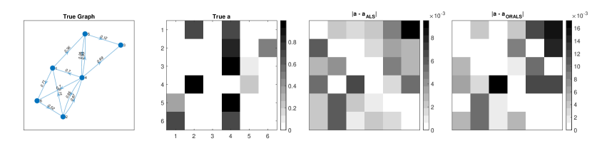
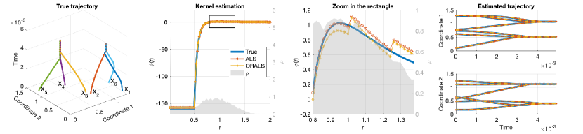
Figure 2: Top: a typical weight matrix estimation. The first two columns show the true graph and its weight matrix. The two columns on the right show the entry-wise errors of the ALS and ORALS estimators. Bottom: Estimator of interaction kernel and trajectory prediction. The left column shows a true trajectory. The middle two columns show the true and estimated kernels with a zoom-in to show the details in a rectangular region. The fourth column presents the true (the same as in column 1) and predicted trajectories. Note that $X_{3}$ and $X_{2}$ do not converge to the same cluster, in both the true and estimated trajectory, even though they are close at time 0, since there are no edges between them in the graph.

	Graph error $\varepsilon_{\mathbf{a}}$	Kernel error $\varepsilon_{K}$	Traj. error $\varepsilon_{\mathbf{X}}$	Exp. traj. error $\varepsilon_{\mathbf{X}}$
ALS	$8.47\times 10^{-3}$	$1.45\times 10^{-2}$	$6.1\times 10^{-3}$	$6.19\times 10^{-3}\pm 8.12\times 10^{-4}$
ORALS	$1.67\times 10^{-2}$	$1.47\times 10^{-2}$	$6.6\times 10^{-3}$	$7.41\times 10^{-3}\pm 1.07\times 10^{-3}$

Table 3: Error of the estimators in Figure 2 in a typical simulation, and, in the fourth column, mean and SD of trajectory prediction errors of 100 random trajectories.

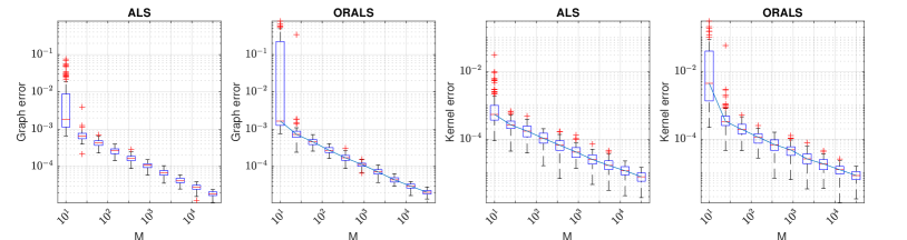
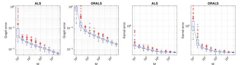
Figure 3: Convergence with sample size M increasing in 100 independent experiment runs. The top row shows almost perfect rates of $M^{-1/2}$ for both algorithms for the case of noiseless data and a well-specified basis. For the case of noisy data and misspecified basis, the bottom row shows robust convergence with the errors decaying until they reach $10^{-4}$, the variance of observation noise.

3.2 Convergence in sample size

Rate of convergence and robustness.

We examine the estimators’ convergence rates in sample size $M$ and their robustness to basis misspecification and noise in data. Thus, we consider two cases: a case with noiseless data and a well-specified basis $\{\psi_{1},\psi_{4},\psi_{7}\}$, which we aim to show the convergence rate of $M^{-1/2}$ as proved for the parametric setting; and a case with noisy data with $\sigma_{obs}=10^{-2}$ and the above basis functions $\{\psi_{k}\}_{k=1}^{7}$, which we aim to test the robustness of the convergence.

Figure 3 shows that both ALS and ORALS yield convergent estimators as the sample size $M$ increases. Here, the data trajectories are generated from the system with a stochastic force with $\sigma=10^{-2}$. In either case, the boxplots show the relative errors in 100 random simulations. In each simulation, we compute a sequence of estimators from $M$ sample trajectories, where $M\in\{10,24,59,146,359,879,2154,5274,12915,31622\}$. In each boxplot, the central mark indicates the median, and the bottom and top edges of the box indicate the 25th and 75th percentiles, respectively. The whiskers extend to the most extreme data points not considered outliers, and the outliers are plotted individually using the “+” marker symbol.

In the case of noiseless data and well-specified basis, the top row shows nearly perfect decay rates of $M^{-1/2}$ for both the graph errors and the kernel errors and for both ALS and ORALS algorithms. For ORALS, this convergence rate agrees with Theorem 2.7. ALS has similar convergence rates, even though it does not have a theoretical guarantee for convergence.

In the case of noisy data and misspecified basis, as shown in the bottom row, the decay rate remains clear for the graph errors, but the kernel errors decay at a rate slightly slower than $M^{-1/2}$ before reaching the level of observation noise $\sigma_{obs}^{2}=10^{-4}$. ALS’s graph errors are about half a digit smaller than the ORALS’ graph errors; while both algorithms lead to similar kernel errors when the sample size is large, the ALS’ kernel errors are much smaller when the sample size is small. Thus, ALS is more robust to noise and misspecification than ORALS, and it can lead to reasonable estimators even if the sample size is small, which we further examine next.

Behavior of the estimators as a function of $M$ and $L$.

We further examine the performance of our estimators as a function of the number of sample paths $M$ and the trajectory length $L$, so that the total number of observations is $ML$, each a $d$-dimensional vector. Here we consider an interaction kernel $\Phi(x)=\phi(|x|)\frac{x}{|x|}$ with $\phi(r)=\sum_{k=1}^{p}w_{k}/k\sin(2\pi kr)/(r+0.1)$, where $w_{k}\overset{\mathrm{i.i.d.}}{\sim}\mathcal{N}(0,1)$.

Figure 4 shows the results for $N=32$, $p=16$, $d=1$, $\sigma=10^{-4}$ and observation noise $10^{-4}$. The top panel shows the results with $L=2$ (left) and $L=8$ (right). The first dashed vertical bar is in correspondence of $M=(N^{2}+{p})/(NL)$ (left) and $M=(N^{2}+{p})/(NL/2)$ (right); the second dashed vertical bar is at $M=(N^{2}{p})/(NL)$: since we have a total of $MLdN$ scalar observations, and $N^{2}+{p}$ parameters to estimate, the first one corresponds to a nearly information-theoretic optimal sampling complexity, and we see that ALS appears to start performing well around that level of samples, albeit, because of the lack of independence in $L$, on the right we have to multiply by $2$; the second one appears to be consistent with the sample size at which ORALS starting to get a good performance. In the small and medium sample regime, between the two vertical bars, ALS significantly and consistently outperforms ORALS; for large sample sizes, the two estimators have similar performance.

The bottom panel shows the performance of the ALS estimator as a function of both $M$ and $L$ (recall that $T=Ldt$). The performance improves not only as $M$ increases but also as $L$ increases, at least for this particular system.

The main takeaways are that (i) ALS appears to achieve good performance as soon as the number of samples is comparable to $(N^{2}+{p})/(Ld)$ (after what might be a phase transition from the phase where the samples are insufficient), while the number for ORALS is of order $(N^{2}{p})/(Ld)$; (ii) the effective sample size, at least for this dynamics, appears to increase with $L$, and perhaps as fast as the product $ML$, notwithstanding the dependence between samples along a single trajectory.

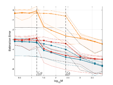
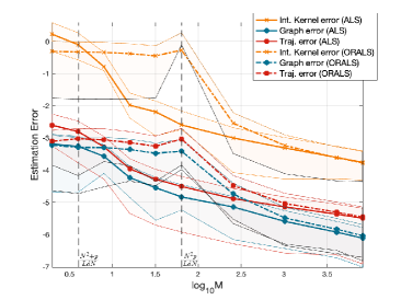
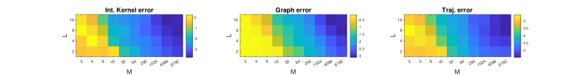
Figure 4: Top: Estimation errors as a function of $M$ (with all other parameters fixed), for both ALS and ORALS, for a random Fourier interaction kernel with $p=16$, $N=32$, $L=2$ (left) and $L=8$ (right). In the small and medium sample regime, between the two vertical bars, ALS significantly and consistently outperforms ORALS; for large sample sizes, the two estimators have similar performance. Bottom: The performance of the ALS estimator improves not only as $M$ increases but also as $L$ increases.

3.3 Dependence on noise level and stochastic force

Numerical tests also show that the estimator’s error decays linearly in the scale of the stochastic force and the noise level. The linear decay rate in the scale of the stochastic force agrees with Theorem 2.7, where the variance of the error for the ORALS estimator is proportional to $\sigma^{2}$. We refer to Sect.B.3 for details.

4 Applications

4.1 Kuramoto model on network, with misspecified hypothesis spaces

We consider the Kuramoto model with network

$$d{X}^{i}_{t}={\kappa}\sum_{j\in\mathcal{N}_{i}}a_{ij}\sin(X^{j}_{t}-X^{i}_{t})dt+\sigma d{W}^{i}_{t},\quad i=1,\ldots,N.$$ (4.1)

When $a_{ij}\equiv 1$ and $\sigma=0$, it reduces to the classical Kuramoto model of N coupled oscillators, where $X_{t}^{i}$ represents the phase of the $i$-th oscillator. Here $\kappa$ represents the coupling constant. The Kuramoto model was introduced to study the behavior of systems of chemical and biological oscillators [Kur75] and has been extended to study flocking, schooling, vehicle coordination, and electric power networks (see [DB14, GFR⁺22] and the reference therein).

In this example, our goal is to jointly estimate from multi-trajectory data the weight matrix $\mathbf{a}$, and the coefficient $c$ of the (true) interaction kernel $\Phi(x)=\sin(x)$ over the misspecified hypothesis space

$$\mathcal{H}=\mathrm{span}\{\cos(x),\sin(2x),\cos(2x),\dots,\cos(7x),\sin(7x)\}\,,$$

which does not contain $\Phi$, and over the hypothesis space $\mathcal{H}_{\phi}:=\mathrm{span}\{\mathcal{H},\Phi\}$.

We consider a system with $N=10$ oscillators, using the uniform distribution over the interval $[-2,2]$ as the initial distribution, as well as a stochastic force with $\sigma=10^{-4}$, an observation noise with $\sigma_{obs}=10^{-3}$, time $T=0.1$ and $\Delta t=0.001$ (therefore, $L=100$). We compare the kernel estimation result using $\mathcal{H}$ and $\mathcal{H}_{\phi}$, with the number of observed trajectories $M\in\{8,64,512\}$. In Figure 5, we present the true graph and a typical trajectory; in particular, we present the kernel estimators’ mean, with one SD range represented by the shaded region, from 20 independent simulations. The successful joint estimation results suggest ALS and ORALS may overcome the discrepancy between the true kernel and the hypothesis space, making them applicable to nonparametric estimation.

Due to the network structure, the system can have interesting synchronization patterns. The bottom left of Figure 5 shows an example of such a pattern: groups of particles moving in clusters, with each cluster having a similar angular velocity robust to the perturbation by the stochastic force. These synchronization patterns appear dictated by the network structure, and appear robust to the initial condition. In general, it is nontrivial to predict when these synchronization patterns emerge and what their features are depending on the network; for a recent study in the case of random Erdös-Rényi graphs, we refer the reader to [ABK⁺23] and references therein.

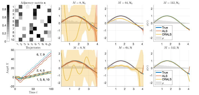
Figure 5: The first column shows the true weight matrix $\mathbf{a}$ and a trajectory of the system with an interesting clustering pattern. In the remaining columns, we show the estimators of the interaction function with misspecified and well-specified hypothesis spaces, i.e., $\phi\notin\mathcal{H}$ (top row) and $\phi\in\mathcal{H}_{\phi}$ (bottom row) respectively, with M ranging in $[8,64,521]$. Our estimators appear robust to basis misspecification, albeit with performance worse than in the well-specified case.

4.2 Estimating a leader-follower network

Consider the problem of identifying the leaders and followers in a system of interacting agents from trajectory data. In this system, the leader agents make a stronger influence through more connections to other agents than the follower agents. Such a system can describe opinion dynamics on social network [WS06, MT14, DTW18, HZBL⁺20] and collective motion of pigeon flocks [NÁBV10]. We consider the following leader-follower model

$$d{X}^{i}_{t}=\sum_{j\neq i}\mathbf{a}_{ij}\Phi(X^{j}_{t}-X^{i}_{t})dt+\sigma d{W}^{i}_{t},\quad i=1,\ldots,N$$ (4.2)

where the true interaction kernel (named influence function in the opinion dynamics literature)

$$\Phi(x)=-\Phi_{1}(x)-0.1\Phi_{2}(x)$$

with the bases $\Phi_{1}(x)=\mathbbm{1}_{\{x\leq 1\}}$ and $\Phi_{2}(x)=\mathbbm{1}_{\{1<x\leq 1.5\}}$. The weight matrix $\mathbf{a}$ represents a leadership network, with the weights on the directed edges to be understood as a measure of impact or influence.

We identify the agents as leaders or followers by first estimating the weight matrix $\mathbf{a}$ from data by the ALS algorithm and then using the $K$-means method (e.g., [Bis06, Chapter 9]) to analyze the impact feature and the influence feature extracted from the matrix. The detailed algorithm of clustering is presented as follows.

Step 1: Identify the leaders. Given the weight matrix, observe that for any agent $A_{i}$, the row-wise sum $\|\mathbf{a}_{i\cdot}\|_{\ell_{1}}=\sum_{j\neq i}|\mathbf{a}_{ij}|$ represents its impact on other agents in the system, and the column-wise sum $\|\mathbf{a}_{\cdot i}\|_{\ell_{1}}=\sum_{j\neq i}|\mathbf{a}_{ji}|$ corresponds to the influence of the system on $i$. We posit that leadership can be characterized as the linear combination of impact on the system and influence from others:

$$L_{i}=\alpha\|\mathbf{a}_{i\cdot}\|_{\ell_{1}}+\beta\|\mathbf{a}_{\cdot i}\|_{\ell_{1}}\,,\quad\text{with }\alpha+\beta=1\,,\alpha>\beta\,,$$ (4.3)

Typically, the impact factor $\alpha$ is expected to surpass the influence factor $\beta$ when discussing leadership. Subsequently, we identify the leaders and followers by applying the $K$-means method to cluster the leadership features $\{L_{i}\}_{i=1}^{N}$. We represent leaders and followers by a partition of the index set: $[N]=S_{1}\bigcup S_{2}=\{i_{1},\cdots,i_{\widetilde{N}}\}\bigcup\{j_{1},\cdots,j_{\widetilde{N}^{\prime}}\}$ with $N=\widetilde{N}+\widetilde{N}^{\prime}$, representing leaders and followers, respectively.

Step 2: Classify the Followers. We further classify each follower in a group according to his or her leader. We start by setting the $\widetilde{N}$ groups to be $\{G^{1}=\big{\{}i_{1}\},\cdots,G^{\widetilde{N}}=\{i_{\widetilde{N}}\}\big{\}}$. To classify follower $j\in S_{2}$, we consider another leadership feature:

$$\widetilde{L}_{j}^{k}=\alpha\sum_{i\in G^{k}}|\mathbf{a}_{ij}|+\beta\sum_{i\in G^{k}}|\mathbf{a}_{ji}|\,,\quad\forall\leavevmode\nobreak\ k=1,\cdots,{\widetilde{N}}\,.$$

Then we find the largest $\widetilde{L}_{j}^{k_{0}}$ and classify agent $j$ to group $k_{0}$ and set this group to be $\{G^{k_{0}},j\}$. We continue this procedure until all followers are classified.

Figure 6 demonstrates the identified network of the agents via the above method with $(\alpha,\beta)=(0.8,0.2)$. In this experiment, we have two leaders, labeled as $A1$ (red group) and $A6$ (blue group), out of $N=20$ agents, and we consider three sample sizes $M\in\{15,30,100\}$. The figure shows the identification of the leader-follower network depends on sample size: we can identify the leader-follower network accurately when the sample size is large, e.g., $M=100$. The error of graph estimation is $0.0018$. But when the sample is too small, e.g., $M=15$ and $M=30$, the inference can have large errors: the errors of graph estimation are $0.1254$ when $M=15$ and $0.0094$ when $M=30$. Nevertheless, the leaders and followers are correctly identified; see more detailed results in Appendix B.5.

This example suggests that we can consistently identify and cluster leaders and followers from a small sample size.

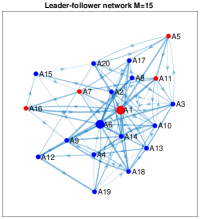
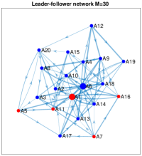
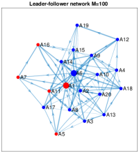
Figure 6: Estimated networks of leaders and followers from datasets with sample sizes $M\in\{15,30,100\}$ and the ground truth. When $M=100$, the estimated network is accurate. When $M=30$, the leaders-follower network is correctly identified, though the weight matrix is less accurate. When $M=15$, the sample size is too small for a meaningful inference; but the clustering is still reliable.

4.3 Multitype interaction kernels

We consider further the joint inference of a generalized model with multiple types of agents distinguished by their interaction kernels. Specifically, consider a system with $Q$ types of interaction kernels, and denote by $\kappa(i)$ the type of kernel for the agent $i$:

$$\mathcal{S}_{{\mathbf{a}},{(\Phi_{q})_{q=1}^{Q},\kappa}}\,:\qquad d{X}^{i}_{t}=\sum_{j\neq i}\mathbf{a}_{ij}\Phi_{\kappa(i)}(X^{j}_{t}-X^{i}_{t})dt+\sigma d{W}^{i}_{t},\quad i=1,\ldots,N\,,$$ (4.4)

where $\Phi_{q}$ is the interaction kernel for agents of type $q$. Given a hypothesis space $\mathcal{H}=\text{span}\{\psi_{k}\}_{k=1}^{p}$ that includes these kernels, there a exists coefficients matrix $\mathbf{c}\in\mathbb{R}^{p\times N}$ such that

$$\Phi_{\kappa(i)}(x)=\sum_{k=1}^{p}\mathbf{c}_{ki}\psi_{k}(x)$$

with $\mathbf{c}_{\cdot i}=\mathbf{c}_{\cdot j}$ if $\kappa(i)=\kappa(j)$, namely the matrix $\mathbf{c}$ has $Q$ distinct columns. Using the same tensor notation as before, we have

$$\mathcal{S}_{{\mathbf{a}},{\mathbf{c}}}\quad: \dot{\mathbf{X}}_{t}=\mathbf{a}\mathbf{B}(\mathbf{X}_{t})\mathbf{c}+\sigma\dot{\mathbf{W}}=\big{(}\mathbf{a}_{i\cdot}\mathbf{B}(\mathbf{X}_{t})_{i}\mathbf{c}_{\cdot i}\big{)}_{i\in[N]}+\sigma\dot{\mathbf{W}}\,,\quad\text{ where}$$ (4.5)

$$\mathbf{a}_{i\cdot}\mathbf{B}(\mathbf{X}_{t})_{i}\mathbf{c}_{\cdot i}=\sum_{j\neq i}\mathbf{a}_{ij}\sum_{k=1}^{p}\psi_{k}(X^{j}_{t}-X^{i}_{t})c_{ki}\in\mathbb{R}^{d}\,,i\in[N].$$

Our goal is to jointly estimate the weight matrix $\mathbf{a}$ and the matrix $\mathbf{c}$, which represents the $Q$ kernels without knowing the type function $\kappa$, from data consisting of multiple trajectories.

Since $\mathbf{c}$ has $Q$ distinct columns, we have $\text{rank}(\mathbf{c})\leq Q$, which is a weaker condition. However, the low-rank property of $\mathbf{c}$ is sufficient for us to apply the idea of ALS. Using SVD on $\mathbf{c}$, we can decompose $\mathbf{c}$ as

$$\mathbf{c}=\textbf{u}\textbf{v}^{\rm T}$$ (4.6)

where $\textbf{u}\in\mathbb{R}^{p\times Q}$ is called the coefficient matrix. This is because u represents the orthogonalized coefficients of the $Q$ interaction kernels on the basis $\{\psi_{k}\}$. And the type matrix ${\textbf{v}}\in R^{N\times Q}$ is assumed to be orthonormal, i.e., $\textbf{v}^{\rm T}\textbf{v}=I_{Q}$, as it represents the type of the $i$-th particle with each row of v represents the weight of the orthogonalized $Q$ interaction kernels that the kernel $\Phi_{\kappa(i)}$ has. Such normalization condition avoids the simple non-identifiability issue, as demonstrated in the admissible set of $\mathbf{a}$. We write the above system as

$$\mathcal{S}_{{\mathbf{a}},{\textbf{u},\textbf{v}}}\quad: \dot{\mathbf{X}}_{t}=\mathbf{a}\mathbf{B}(\mathbf{X}_{t})\textbf{u}\textbf{v}^{\rm T}+\sigma\dot{\mathbf{W}}=\big{(}\mathbf{a}_{i\cdot}\mathbf{B}(\mathbf{X}_{t})_{i}\textbf{u}\textbf{v}_{i\cdot}^{\rm T}\big{)}_{i\in[N]}+\sigma\dot{\mathbf{W}}\,,\quad\text{ where}$$ (4.7)

$$\mathbf{a}_{i\cdot}\mathbf{B}(\mathbf{X}_{t})_{i}\textbf{u}\textbf{v}_{i\cdot}^{\rm T}=\sum_{j\neq i}\mathbf{a}_{ij}\sum_{k=1}^{p}\psi_{k}(X^{j}_{t}-X^{i}_{t})\sum_{q=1}^{Q}\textbf{u}_{kq}\textbf{v}_{iq}\in\mathbb{R}^{d}\,,i\in[N].$$

With data of multiple trajectories $\{\mathbf{X}_{t_{0}:t_{L}}^{m}\}_{m=1}^{M}$, the loss function is defined as

$$(\widehat{\mathbf{a}},\widehat{\textbf{u}},\widehat{\textbf{v}}) =\underset{\begin{subarray}{c}(\mathbf{a},\textbf{u},\textbf{v})\in\mathcal{M}\times\mathbb{R}^{p\times Q}\times\mathbb{R}^{N\times Q}\\ \textbf{v}^{\rm T}\textbf{v}=I_{Q}\end{subarray}}{\operatorname{arg}\operatorname{min}}\;\mathcal{E}_{L,M}(\mathbf{a},\textbf{u},\textbf{v}),\,\,\,\text{ with}$$ (4.8)

$$\mathcal{E}_{L,M}(\mathbf{a},\textbf{u},\textbf{v}) :=\frac{1}{MT}\sum_{l=1,m=1}^{L,M}\left\|\Delta\mathbf{X}_{t_{l}}^{m}-\mathbf{a}\mathbf{B}(\mathbf{X}_{t_{l}}^{m})\textbf{u}\textbf{v}^{\rm T}\Delta t\right\|_{F}^{2},$$

We introduce a three-fold ALS algorithm to solve the above optimization problem. Notice that the loss function (4.8) is quadratic in each of the unknowns $\mathbf{a},\textbf{u},\textbf{v}$ if we fix the other two. The three-fold ALS algorithm alternatively solves for each of the unknowns while fixing the other two. In each iteration, this algorithm proceeds as follows: solving $\mathbf{a}$ via least squares with nonnegative constraints, next solving u by least square, and then solving v via least squares followed by an ortho-normalization step, which is an orthogonal Procrustes problem [GD04]. Additionally, we add an optional $K$-means step to ensure that $\mathbf{c}$ has only $Q$ distinct columns. The details of the algorithm are postponed to Section D.

Figure 7 numerically compares the three-fold ALS with and without the $K$-means step. Here we consider $Q=2$ types of kernels corresponding to short-range and long-range interactions. We use the data of $M=400$ independent trajectories, with a uniform distribution over the interval $[0,5]$ as initial distribution, $\Delta t=10^{-3},L=50$ so that $T=0.05$, and the stochastic force and the observation noise have $\sigma=\sigma_{obs}=10^{-3}$. The weight matrix is randomly generated with entries sampled from the uniform distribution on $[0,1]$, followed by a row-normalization. The true kernels are constructed on spline basis functions, representing short-range interaction (Type 1) and long-range interaction (Type 2).

Figure 7 reports the error decay in the iteration number and the comparison between the estimated and true kernels. It shows that the algorithm using $K$-means at each step performs better than the one without the $K$-means since it preserves more model information.

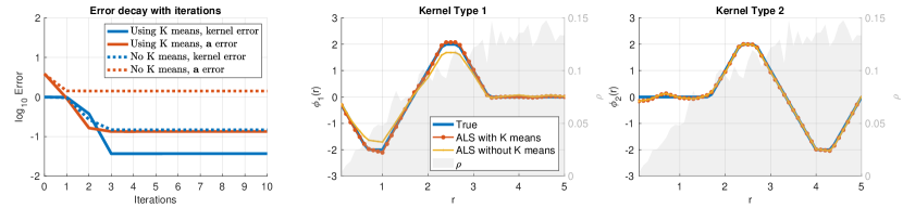
Figure 7: Estimation of two types of kernels: short range and long range. The first panel shows the error decay with respect to iteration numbers. The algorithm using $K$-means decays faster and reaches lower errors than the algorithm without $K$-means. The right two columns show the estimation result of the two kernels. The classification is correct for both of the algorithms, and the one with $K$-means yields more accurate estimators, particularly for the kernel Type 1.

Model selection.

We further test the robustness of the three-fold ALS algorithm for model selection when the number $Q\in\{1,2\}$ is unknown. We apply the algorithm with both $Q\in\{1,2\}$ on two datasets that are generated with $Q_{true}=1$ and $Q_{true}=2$ respectively. Table 4 shows that the three-fold ALS can select the correct model through trajectory prediction errors. It reports the means and SDs of trajectory prediction using $10$ test trajectories, $\Delta t=10^{-2}$ and $L=500$ time steps. Note that the total time length is $T=5$. When $Q_{true}=1$, the error of the estimators with misspecified $Q=2$ is relatively accurate, because the estimated two types of kernels are both close to the true kernel, as examined in Figure 8. Thus, the algorithm effectively identifies the correct model.

	$Q_{true}=1$	$Q_{true}=2$
Estimated with $Q=1$	$1.22\times 10^{-2}\pm 8.23\times 10^{-3}$	$2.06\times 10^{-1}\pm 6.88\times 10^{-2}$
Estimated with $Q=2$	$1.44\times 10^{-2}\pm 7.40\times 10^{-3}$	$1.12\times 10^{-2}\pm 2.80\times 10^{-3}$

Table 4: Model selection: single- v.s. two- types of kernels. The table shows the Mean and SD of trajectory prediction errors in 10 independent numerical experiments, where the number of kernel types is unknown. Smaller errors indicate a correct model. The model is correctly identified in both cases (highlighted in bold).

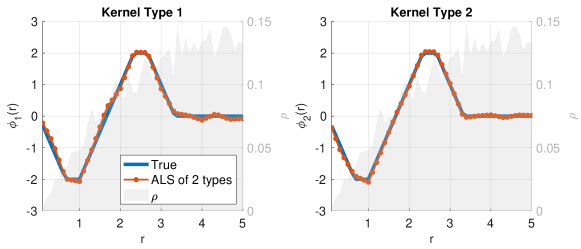
Figure 8: Estimated kernels in a misspecified case: estimating two types of kernel when data is generated using a single kernel. The algorithm outputs two types of kernels, but both are close to the true kernel.

5 Conclusion

We have proposed a robust estimator for joint inference of networks and interaction kernels in interacting particle systems on networks, implemented with computationally two scalable algorithms: ALS and ORALS. We have tested the algorithms on several classes of systems, including deterministic and stochastic systems with various types of networks and with single and multi-type kernels. We have also examined the non-asymptotic and asymptotic performance of the algorithms: the ALS is robust for small sample sizes and misspecified hypothesis spaces, and both algorithms yield convergent estimators in the large sample limit.

Our joint inference problem leads to a non-convex optimization problem that resembles those in compressed sensing and matrix sensing. However, diverging from the conventional framework of matrix sensing, our data are correlated, our joint estimation is in a constrained parameter space and a function space, and the Restricted Isometry Property (RIP) condition rarely holds with a small RIP constant. These differences can lead to an optimization landscape with multiple local minima.

We introduce coercivity conditions that guarantee the identifiability and the well-posedness of the inverse problem. These conditions also ensure that the ALS and ORALS algorithms have well-conditioned regression matrices and the asymptotical normality for the ORALS estimator. Also, we have established connections between the coercivity and RIP conditions, providing insights into further understanding of the joint estimation problem.

Interacting particle systems on networks offer a wide array of versatile models applicable across multiple disciplines. These include estimating the Kuramoto model on a network, classifying agent roles within leader-follower dynamics, and learning systems with multiple types of interaction kernels. Our algorithms are adaptable to various scenarios and applications and amenable to be extended to more general settings, including models with more general interaction kernels.

We expect further applications of the algorithms for the construction of effective reduced heterogeneous models for large multi-scale systems. Also, other future directions include generalizations to nonparametric joint estimations, further understanding of the convergence and stability of the ALS algorithm, regularizations enforcing the low-rank structures, and learning from partial observations.

Appendix A Theoretical analysis

A.1 Coercivity conditions: connections and examples

First, we present the proof of Proposition 2.3, which states that the rank-2 joint coercivity implies identifiability.

Proof of Proposition 2.3. Notice that

$$\mathcal{E}_{L,\infty}^{(i)}(\mathbf{a},\Phi):= \mathbb{E}\bigg{[}\bigg{|}\sum_{j\neq i}[\mathbf{a}_{ij}^{*}\Phi_{*}(\mathbf{r}_{ij}(t_{l}))-\mathbf{a}_{ij}\Phi(\mathbf{r}_{ij}(t_{l}))]\bigg{|}^{2}\bigg{]}$$

$$= \mathbb{E}\bigg{[}\bigg{|}\sum_{j\neq i}\Big{[}\mathbf{a}_{ij}^{*}-p_{\Phi}\mathbf{a}_{ij}\Big{]}\Phi_{*}(\mathbf{r}_{ij}(t_{l}))+\mathbf{a}_{ij}\Big{[}p_{\phi}\Phi_{*}(\mathbf{r}_{ij}(t_{l}))-\Phi(\mathbf{r}_{ij}(t_{l}))\Big{]}\bigg{|}^{2}\bigg{]}$$

where

$$p_{\Phi}=\frac{\langle{\Phi,\Phi_{*}}\rangle_{\rho_{L}}}{\|\Phi_{*}\|_{\rho_{L}}^{2}}\,,\quad\text{and}\quad p_{\Phi}\Phi_{*}-\Phi\perp\Phi_{*}\text{ in }\mathcal{H}.$$

Therefore, from rank-2 joint coercivity condition (2.10) we have

$$\mathcal{E}_{L,\infty}^{(i)}(\mathbf{a},\phi) \geq c_{\mathcal{H}}|\mathbf{a}_{i\cdot}^{*}-p_{\phi}\mathbf{a}_{i\cdot}|^{2}\|\phi_{*}\|_{\rho_{L}}^{2}+c_{\mathcal{H}}|\mathbf{a}_{i\cdot}|^{2}\|p_{\phi}\Phi_{*}-\Phi\|_{\rho_{L}}^{2}\,.$$ (A.1)

Hence $\mathcal{E}_{L,\infty}(\mathbf{a},\Phi)=\sum_{i}\mathcal{E}_{L,\infty}^{(i)}(\mathbf{a},\Phi)=0$ and $c_{\mathcal{H}}>0$ imply that

$$|\mathbf{a}_{i\cdot}^{*}-p_{\Phi}\mathbf{a}_{i\cdot}|^{2}=0\,,\quad\text{and}\quad\|p_{\Phi}\Phi_{*}-\Phi\|_{\rho_{L}}^{2}=0\,,\forall i\in[N],$$

since $\Phi_{*}\neq 0$ and $0\neq\mathbf{a}\in\mathcal{M}$. Because $\mathbf{a}^{(*)},\mathbf{a}\in\mathcal{M}$, the only choice for $|\mathbf{a}_{i\cdot}^{*}-p_{\Phi}\mathbf{a}_{i\cdot}|^{2}=0$ is both $p_{\Phi}=1$ and $\mathbf{a}^{*}=\mathbf{a}$. Consequently, $\|p_{\Phi}\Phi_{*}-\Phi\|_{\Phi_{L}}^{2}=\|\Phi_{*}-\Phi\|_{\rho_{L}}^{2}=0$ yields $\Phi_{*}=\Phi$ in $L^{2}_{\rho}$.   

The next proposition implies that the interaction kernel coercivity is stronger than the joint coercivity.

Proposition A.1 (Interaction kernel coercivity implies joint coercivity)

Assume that for all $i\in[N]$, $\{\mathbf{r}_{ij}(t)=X_{t}^{j}-X_{t}^{i}\}_{j=1,j\neq i}^{N}$ are pairwise independent conditional on $\mathcal{F}^{i}_{t}$. Then, the kernel coercivity (2.11) with $c_{0,\mathcal{H}}$ implies that the joint coercivity conditions (2.9) and (2.10) hold with $c_{1,\mathcal{H}}=C_{\mathbf{a},N}^{(1)}c_{0,\mathcal{H}}$ and $c_{2,\mathcal{H}}=C_{\mathbf{a},N}^{(2)}c_{0,\mathcal{H}}$, respectively, where $C_{\mathbf{a},N}^{(1)}=\frac{1}{N}\sum_{i=1}^{N}\sum_{j\neq i}\mathbf{a}_{ij}^{2}$ and $C_{\mathbf{a},N}^{(1)}=\frac{1}{N}\sum_{i=1}^{N}\sum_{j\neq i}[|\mathbf{a}_{ij}^{(1)}|^{2}+|\mathbf{a}_{ij}^{(2)}|^{2}]$.

Proof. Without loss of generality, we consider only the case when $L=1$. By assumption, the random variables $\mathbf{r}_{ij}$ and $\mathbf{r}_{ij^{\prime}}$ are independent, conditioned on $\mathcal{F}^{i}$, if $j\neq j^{\prime}$ and $j,j^{\prime}\neq i$. Then, by Lemma A.3 with $f_{j}(\cdot)=\mathbf{a}_{ij}\Phi(\cdot)$ for each fixed $i$, we get

$$\frac{1}{N}\sum_{i=1}^{N}\mathbb{E}\bigg{[}\bigg{|}\sum_{j\neq i}\mathbf{a}_{ij}\Phi(\mathbf{r}_{ij})\bigg{|}^{2}\bigg{]} =\frac{1}{N}\sum_{i=1}^{N}\mathbb{E}\bigg{[}\mathbb{E}\bigg{(}\bigg{|}\sum_{j\neq i}\mathbf{a}_{ij}\Phi(\mathbf{r}_{ij})\bigg{|}^{2}\mid\mathcal{F}^{i}\bigg{)}\bigg{]}$$

$$\geq\frac{1}{N}\sum_{i=1}^{N}\sum_{j\neq i}\mathbf{a}_{ij}^{2}\mathbb{E}[\mathrm{tr\,Cov}(\Phi(\mathbf{r}_{ij})\mid\mathcal{F}^{i})]$$

$$\geq\frac{1}{N}\sum_{i=1}^{N}\sum_{j\neq i}\mathbf{a}_{ij}^{2}c_{0,\mathcal{H}}\|\Phi\|_{\rho_{L}}^{2}=C_{\mathbf{a},N}^{(1)}c_{0,\mathcal{H}}\|\Phi\|_{\rho_{L}}^{2}\,,$$

where the last inequality follows from (2.11). Therefore, by combining the above inequalities, we obtain that (2.9) holds with the constant $c_{1,\mathcal{H}}=C_{\mathbf{a},N}^{(1)}c_{0,\mathcal{H}}$. This proves the rank-1 joint coercivity condition.

We proceed to prove the rank-2 joint coercivity condition (2.10). It suffices to show that for all $i\in[N]$,

$$\mathbb{E}\bigg{[}\bigg{|}\sum_{j\neq i}[\mathbf{a}_{ij}^{(1)}\Phi_{1}(\mathbf{r}_{ij})+\mathbf{a}_{ij}^{(2)}\Phi_{2}(\mathbf{r}_{ij})]\bigg{|}^{2}\bigg{]}\geq c_{2,\mathcal{H}}\left[|\mathbf{a}_{i\cdot}^{(1)}|^{2}\|\Phi_{1}\|_{\rho_{L}}^{2}+|\mathbf{a}_{i\cdot}^{(2)}|^{2}\|\Phi_{2}\|_{\rho_{L}}^{2}\right]\,,$$ (A.2)

for any vectors $\mathbf{a}_{i\cdot}^{(1)},\mathbf{a}_{i\cdot}^{(2)}\in\mathcal{M}$ and any two functions $\Phi_{1},\Phi_{2}\in\mathcal{H}$ with $\langle\Phi_{1},\Phi_{2}\rangle=0$. As in the rank-1 case, we have by Lemma A.3 that

$$\mathbb{E}\bigg{[}\bigg{|}\sum_{j\neq i} [\mathbf{a}_{ij}^{(1)}\Phi_{1}(\mathbf{r}_{ij})+\mathbf{a}_{ij}^{(2)}\Phi_{2}(\mathbf{r}_{ij})]\bigg{|}^{2}\bigg{]}$$

$$=\sum_{j\neq i}|\mathbf{a}_{ij}^{(1)}|^{2}\mathbb{E}[\mathrm{tr\,Cov}(\Phi_{1}(\mathbf{r}_{ij})\mid\mathcal{F}^{i})]+\sum_{j\neq i}|\mathbf{a}_{ij}^{(2)}|^{2}\mathbb{E}[\mathrm{tr\,Cov}(\Phi_{2}(\mathbf{r}_{ij})\mid\mathcal{F}^{i})]$$

$$+\mathbb{E}\left[\bigg{|}\sum_{j\neq i}\mathbf{a}_{ij}^{(1)}\mathbb{E}\big{[}\Phi_{1}(\mathbf{r}_{ij})\mid\mathcal{F}^{i}\big{]}\bigg{|}^{2}\right]+\mathbb{E}\left[\bigg{|}\sum_{j\neq i}\mathbf{a}_{ij}^{(2)}\mathbb{E}\big{[}\Phi_{2}(\mathbf{r}_{ij})\mid\mathcal{F}^{i}\big{]}\bigg{|}^{2}\right]$$

$$+2\mathbb{E}\left[\sum_{j\neq i}\mathbf{a}_{ij}^{(1)}\mathbb{E}\Big{[}\Phi_{1}(\mathbf{r}_{ij})\mid\mathcal{F}^{i}\Big{]}\cdot\sum_{j\neq i}\mathbf{a}_{ij}^{(2)}\mathbb{E}\Big{[}\Phi_{2}(\mathbf{r}_{ij})\mid\mathcal{F}^{i}\Big{]}\right]$$

$$\geq\sum_{j\neq i}|\mathbf{a}_{ij}^{(1)}|^{2}\mathbb{E}[\mathrm{tr\,Cov}(\Phi_{1}(\mathbf{r}_{ij})\mid\mathcal{F}^{i})]+\sum_{j\neq i}|\mathbf{a}_{ij}^{(2)}|^{2}\mathbb{E}[\mathrm{tr\,Cov}(\Phi_{2}(\mathbf{r}_{ij})\mid\mathcal{F}^{i})]\,.$$

This confirms (A.2) holds with the coercivity constant $c_{2,\mathcal{H}}=C_{\mathbf{a},N}^{(2)}c_{0,\mathcal{H}}$ where $C_{\mathbf{a},N}^{(2)}=\frac{1}{N}\sum_{i=1}^{N}\sum_{j\neq i}$ $[|\mathbf{a}_{ij}^{(1)}|^{2}+|\mathbf{a}_{ij}^{(2)}|^{2}]$.   

Remark A.2 (Sufficient but not necessary for identifiability)

Combining with Proposition 2.3, we know that interaction kernel coercivity implies identifiability. Also, we shall see that it is a sufficient condition that we can verify to ensure that the operator regression stage is well-posed. Clearly, we should not expect it to be necessary for the identifiability of the weight matrix and the kernel.

Heuristic, the proof for Proposition A.2 suggests that the kernel coercivity condition (2.11) is not only a sufficient condition for rank-1 and rank-2 joint coercivity but may also imply ‘higher rank’ joint coercivity conditions, suggesting that kernel coercivity resembles with a ‘full rank’ version of the joint coercivity condition.

Lemma A.3

Suppose $\{X^{i}\}_{i=1}^{N}$ are $\mathbb{R}^{d}$-valued random variables such that for each $i$, conditional on an $\sigma$-algebra $\mathcal{F}^{i}$, the random variables $\{\mathbf{r}_{ij}=X^{j}-X^{i}\}_{j=1,j\neq i}^{N}$ are independent. Then, for any square-integrable functions $\{f_{j}:\mathbb{R}^{d}\to\mathbb{R}^{d}\}_{j=1}^{N}$, we have

$$\mathbb{E}\bigg{[}\bigg{|}\sum_{j\neq i}f_{j}(\mathbf{r}_{ij})\bigg{|}^{2}\mid\mathcal{F}^{i}\bigg{]}\geq\sum_{j\neq i}\mathrm{tr\,Cov}\left(f_{j}(\mathbf{r}_{ij})\mid\mathcal{F}^{i}\right)\,,\quad\forall\leavevmode\nobreak\ i\in[N]\,.$$ (A.3)

Proof. It suffices to consider the case $i=1$ as the proofs for different $i$’s are the same. That is, we aim to prove

$$\mathbb{E}\bigg{[}\bigg{|}\sum_{j=2}^{N}f_{j}(\mathbf{r}_{1j})\bigg{|}^{2}\mid\mathcal{F}^{1}\bigg{]}\geq\sum_{j=2}^{N}\mathrm{tr\,Cov}\left(f_{j}(\mathbf{r}_{1j})\mid\mathcal{F}^{1}\right)\,.$$

By the conditional independence assumption, we have

$$\mathbb{E}[\langle{f_{j}(\mathbf{r}_{1j}),f_{j^{\prime}}(\mathbf{r}_{1j^{\prime}})}\rangle_{\mathbb{R}^{d}}\mid\mathcal{F}^{1}]=\langle{\mathbb{E}[f_{j}(\mathbf{r}_{1j})\mid\mathcal{F}^{1}],\mathbb{E}[f_{j^{\prime}}(\mathbf{r}_{1j^{\prime}})\mid\mathcal{F}^{1}]}\rangle_{\mathbb{R}^{d}}.$$

Using this fact for the second equation below, we have

$$\mathbb{E}\bigg{[}\bigg{|}\sum_{j=2}^{N}f_{j}(\mathbf{r}_{1j})\bigg{|}^{2}\mid\mathcal{F}^{1}\bigg{]}= \mathbb{E}\bigg{[}\sum_{j=2}^{N}\Big{|}f_{j}(\mathbf{r}_{1j})\Big{|}^{2}+\sum_{\begin{subarray}{c}j,j^{\prime}=2\\ j\neq j^{\prime}\end{subarray}}^{N}\langle{f_{j}(\mathbf{r}_{1j}),f_{j^{\prime}}(\mathbf{r}_{1j^{\prime}})}\rangle_{\mathbb{R}^{d}}\mid\mathcal{F}^{1}\bigg{]}$$

$$= \sum_{j=2}^{N}\mathbb{E}\Big{[}\big{|}f_{j}(\mathbf{r}_{1j})\big{|}^{2}\mid\mathcal{F}^{1}\Big{]}+\sum_{\begin{subarray}{c}j,j^{\prime}=2\\ j\neq j^{\prime}\end{subarray}}^{N}\Big{\langle}\mathbb{E}\big{[}f_{j}(\mathbf{r}_{1j})\mid\mathcal{F}^{1}\big{]},\mathbb{E}\big{[}f_{j^{\prime}}(\mathbf{r}_{1j^{\prime}})\mid\mathcal{F}^{1}\big{]}\Big{\rangle}_{\mathbb{R}^{d}}$$

$$= \sum_{j=2}^{N}\bigg{\{}\mathbb{E}\Big{[}\big{|}f_{j}(\mathbf{r}_{1j})\big{|}^{2}\mid\mathcal{F}^{1}\Big{]}-\bigg{|}\mathbb{E}\Big{[}f_{j}(\mathbf{r}_{1j})\mid\mathcal{F}^{1}\Big{]}\bigg{|}^{2}\bigg{\}}+\bigg{|}\sum_{j=2}^{N}\mathbb{E}\Big{[}f_{j}(\mathbf{r}_{1j})\mid\mathcal{F}^{1}\Big{]}\bigg{|}^{2}\,.$$ (A.4)

Then, we obtain (A.3) with $i=1$ by noticing the fact that $\mathrm{tr\,Cov}(f_{j}(\mathbf{r}_{1j})\mid X^{1})=\Big{[}\mathbb{E}[|f_{j}(\mathbf{r}_{1j})|^{2}\mid\mathcal{F}^{1}]-\big{|}\mathbb{E}[f_{j}(\mathbf{r}_{1j})\mid\mathcal{F}^{1}]\big{|}^{2}\Big{]}$.   

We now show that the interaction kernel coercivity condition holds in $\mathcal{H}=L^{2}_{\rho}$ for radial kernels when $L=1$ and the initial distribution is standard Gaussian.

Proposition A.4

Let $L=1$, $\Phi(x)=\phi(|x|)\frac{x}{|x|}$, and the components of $(X^{1}_{t_{1}},\ldots,X^{N}_{t_{1}})$ be i.i.d. standard Gaussian random vectors in $\mathbb{R}^{d}$. The interaction kernel coercivity condition in (2.11) holds in $\mathcal{H}=L^{2}_{\rho}$ for $d=1,2,3$.

Proof. We first simplify the interaction kernel coercivity condition by using the symmetry of the distribution and $L=1$. Since $\{X^{i}_{t_{1}}\}_{i=1}^{N}$ are identically distributed, so are the random variables $\{\mathbf{r}_{ij}=X^{i}_{t_{1}}-X^{j}_{t_{1}}\}$, and we have $\mathbb{E}[\mathrm{tr\,Cov}(\Phi(\mathbf{r}_{ij})\mid X^{i}_{t_{1}})]=\mathbb{E}[\mathrm{tr\,Cov}(\Phi(\mathbf{r}_{12})\mid X^{1}_{t_{1}})]$ for all $1\leq i\neq j\leq{N}$. Additionally, since since $L=1$, we have $\|\Phi\|_{\rho_{L}}^{2}=\mathbb{E}[|\Phi(\mathbf{r}_{12})|^{2}]$. Consequently, the interaction kernel coercivity condition (2.11) can be written as

$$\frac{1}{(N-1)}\sum_{j\neq i}\mathbb{E}[\mathrm{tr\,Cov}(\Phi(\mathbf{r}_{ij})\mid X^{i}_{t_{1}})]=\mathbb{E}[\mathrm{tr\,Cov}(\Phi(\mathbf{r}_{12})\mid X^{1}_{t_{1}})]\\ \geq c_{\mathcal{H}}^{0}\|\Phi\|_{\rho_{L}}^{2}\,$$

for all $\Phi\in\mathcal{H}$. It is equivalent to

$$\mathbb{E}[\big{|}\mathbb{E}[\Phi(\mathbf{r}_{12})\mid X^{1}_{t_{1}}]\big{|}^{2}]\leq(1-c_{0,\mathcal{H}})\mathbb{E}[|\Phi(\mathbf{r}_{12})|^{2}]$$

by recalling that $\mathbb{E}[\mathrm{tr\,Cov}(\Phi(\mathbf{r}_{12})\mid X^{1}_{t_{1}})]=\mathbb{E}[|\Phi(\mathbf{r}_{12})|^{2}]-\mathbb{E}[\big{|}\mathbb{E}[\Phi(\mathbf{r}_{12})\mid X^{1}_{t_{1}}]\big{|}^{2}]$. Furthermore, since $\{X^{i}_{t_{1}}\}_{i=1}^{N}$ are independent and identical, we have $\mathbb{E}[\big{|}\mathbb{E}[\Phi(\mathbf{r}_{12})\mid X^{1}_{t_{1}}]\big{|}^{2}]=\mathbb{E}[\langle{\Phi(\mathbf{r}_{12}),\Phi(\mathbf{r}_{13})}\rangle]$. Thus, to verify the interaction kernel coercivity condition, we only need to prove

$$\mathbb{E}\left[\langle{\Phi(\mathbf{r}_{12}),\Phi(\mathbf{r}_{13})}\rangle\right]\leq(1-c_{0,\mathcal{H}})\mathbb{E}[|\Phi(\mathbf{r}_{12})|^{2}]\,.$$

In particular, when $\Phi(x)=\phi(|x|)\frac{x}{|x|}$, the above inequality reduces to

$$\mathbb{E}\left[\phi(|\mathbf{r}_{12}|)\phi(|\mathbf{r}_{13}|)\frac{\langle{\mathbf{r}_{12},\mathbf{r}_{13}}\rangle}{|\mathbf{r}_{12}||\mathbf{r}_{13}|}\right]\leq(1-c_{0,\mathcal{H}})\mathbb{E}[|\phi(|\mathbf{r}_{12}|)|^{2}]\,.$$ (A.5)

Next, we prove (A.5) when $\{X^{i}_{t_{1}}\}_{i=1}$ are i.i.d. Gaussian. Recall that if $X,Y\overset{i.i.d.}{\sim}\mu(x)=\frac{1}{(2\pi)^{d/2}}\exp(-|x|^{2}/2)$, then $X-Y\sim\frac{1}{(4\pi)^{d/2}}\exp(-|x|^{2}/4)$ and $|X-Y|\sim\rho(r)=C_{d}r^{d-1}e^{-\frac{r^{2}}{4}}\mathbf{1}_{\{r\geq 0\}}\,,$ where $C_{d}=\frac{1}{2^{d-1}\Gamma(\frac{d}{2})}$ and $\Gamma(\cdot)$ is the Gamma function. In particular, one has $\rho(r)=e^{-\frac{r^{2}}{4}}\mathbf{1}_{\{r\geq 0\}}$ , $\rho(r)=\frac{1}{2}re^{-\frac{r^{2}}{4}}\mathbf{1}_{\{r\geq 0\}}$ and $\rho(r)=\frac{1}{2\sqrt{\pi}}r^{2}e^{-\frac{r^{2}}{4}}\mathbf{1}_{\{r\geq 0\}}$ when $d=1$ ,$d=2$ and $d=3$, respectively.

Without loss of generality, we only need to consider $\mathbb{E}[|\phi(|\mathbf{r}_{12}|)|^{2}]=\|\phi\|_{L^{2}_{\rho}}^{2}=1$. By direct computation, the left-hand side of (A.5) is

$$\mathbb{E}\left[\phi(|\mathbf{r}_{12}|)\phi(|\mathbf{r}_{13}|)\frac{\langle{\mathbf{r}_{12},\mathbf{r}_{13}}\rangle}{|\mathbf{r}_{12}||\mathbf{r}_{13}|}\right] =\frac{1}{(2\sqrt{3}\pi)^{d}}\int_{\mathbb{R}^{2d}}\phi(|u|)\phi(|v|)\frac{\langle u,v\rangle}{|u||v|}e^{-\frac{(|u|^{2}+|v|^{2}-\langle u,v\rangle)}{3}}dudv$$

$$=\frac{1}{(2\sqrt{3}\pi)^{d}}\int_{0}^{\infty}\int_{0}^{\infty}\phi(r)\phi(s)e^{-\frac{(r^{2}+s^{2})}{3}}G_{d}(r,s)r^{d-1}s^{d-1}drds$$ (A.6)

where the second equality follows from a polar coordinate transformation with

$$G_{d}(r,s) =\int_{S^{d-1}}\int_{S^{d-1}}\langle\xi,\eta\rangle e^{\frac{rs}{3}\langle\xi,\eta\rangle}d\xi d\eta\,.$$ (A.7)

We apply Cauchy-Schwarz inequality to (A.6) and $\|\phi\|_{L^{2}_{\rho}}^{2}=1$ to obtain that

$$\mathbb{E}\left[\phi(|\mathbf{r}_{12}|)\phi(|\mathbf{r}_{13}|)\frac{\langle{\mathbf{r}_{12},\mathbf{r}_{13}}\rangle}{|\mathbf{r}_{12}||\mathbf{r}_{13}|}\right]$$

$$\leq \frac{1}{(2\sqrt{3}\pi)^{d}}\bigg{[}\int_{0}^{\infty}\int_{0}^{\infty}|\phi(r)\phi(s)|^{2}e^{-\frac{(r^{2}+s^{2})}{4}}r^{d-1}s^{d-1}drds\bigg{]}^{\frac{1}{2}}$$

$$\qquad\qquad\ \,\cdot\bigg{[}\int_{0}^{\infty}\int_{0}^{\infty}|G_{d}(r,s)|^{2}e^{-\frac{5(r^{2}+s^{2})}{12}}r^{d-1}s^{d-1}drds\bigg{]}^{\frac{1}{2}}$$

$$= \frac{2^{d-1}\Gamma(\frac{d}{2})}{(2\sqrt{3}\pi)^{d}}\bigg{[}\int_{0}^{\infty}\int_{0}^{\infty}|G_{d}(r,s)|^{2}e^{-\frac{5(r^{2}+s^{2})}{12}}r^{d-1}s^{d-1}drds\bigg{]}^{\frac{1}{2}}=:I(d,G_{d})\,.$$ (A.8)

Thus, (A.5) holds with $1-c_{0,\mathcal{H}}\geq I(d,G_{d})$, equivalently, $c_{0,\mathcal{H}}\leq 1-I(d,G_{d})$. We compute $I(d,G_{d})$ when $d=1$, $d=2$ and $d=3$ separately below.

By (A.8), it is easy to see the key is the estimation of $G_{d}(r,s)$ such that $I(d,G_{d})<1$. Notice that $\int_{S^{d-1}}\langle\xi,\eta\rangle e^{\frac{rs}{3}\langle\xi,\eta\rangle}d\xi$ is invariant with respect to any $\eta\in S^{d-1}$. Without loss of generality, we can select $\eta=e_{1}=(1,0,\cdots,0)\in S^{d-1}$ and write (A.7) as

$$G_{d}(r,s) =\int_{S^{d-1}}\int_{S^{d-1}}\langle\xi,e_{1}\rangle e^{\frac{rs}{3}\langle\xi,e_{1}\rangle}d\xi d\eta=|S^{d-1}|\int_{S^{d-1}}\xi_{1}e^{\frac{rs}{3}\xi_{1}}d\xi\,.$$

Case $d=1$: We have $S^{d-1}=\{-1,1\}$ and $|S^{d-1}|=2$. Thus, $G_{1}(r,s)=|S^{d-1}|\int_{S^{d-1}}\xi e^{\frac{rs}{3}\xi}d\xi=2[e^{\frac{rs}{3}}-e^{-\frac{rs}{3}}]$. Plugging in $d=1$ and $G_{1}(r,s)^{2}=4[e^{\frac{2rs}{3}}+e^{-\frac{2rs}{3}}-2]$ into (A.8), we have by symmetry

$$I(d,G_{d}) =\frac{1}{\sqrt{3\pi}}\bigg{[}\int_{0}^{\infty}\int_{0}^{\infty}e^{-\frac{5(r^{2}+s^{2})}{12}}[e^{\frac{2rs}{3}}+e^{-\frac{2rs}{3}}-2]drds\bigg{]}^{\frac{1}{2}}$$

$$=\frac{1}{\sqrt{3\pi}}\bigg{[}\frac{1}{2}\int_{\mathbb{R}^{2}}e^{-\frac{5(r^{2}+s^{2})}{12}+\frac{2rs}{3}}drds-\frac{1}{2}\int_{\mathbb{R}^{2}}e^{-\frac{5(r^{2}+s^{2})}{12}}drds\bigg{]}^{\frac{1}{2}}$$

$$=\frac{1}{\sqrt{3\pi}}\sqrt{2\pi-\frac{6\pi}{5}}=\sqrt{\frac{4}{15}}\,.$$

Hence, (A.5) holds with the coercivity constant $c_{0,\mathcal{H}}\leq 1-\sqrt{\frac{4}{15}}\simeq 0.4836$.

Case $d\geq 2$: We can proceed to write

$$G_{d}(r,s) =|S^{d-1}|\int_{-1}^{1}\int_{\{\sum_{i=2}^{d}\xi_{i}^{2}=1-\xi_{1}^{2}\}}\xi_{1}e^{\frac{rs}{3}\xi_{1}}d\xi=|S^{d-1}||S^{d-2}|\int_{-1}^{1}\xi_{1}(1-\xi_{1}^{2})^{\frac{d-1}{2}}e^{\frac{rs}{3}\xi_{1}}d\xi_{1}$$

$$=|S^{d-1}||S^{d-2}|\int_{0}^{1}\xi(1-\xi^{2})^{\frac{d-1}{2}}[e^{\frac{rs}{3}\xi}-e^{-\frac{rs}{3}\xi}]d\xi$$

where $|S^{n-1}|=\frac{2\pi^{\frac{n}{2}}}{\Gamma(n/2)}$ is the surface area of a $n$-dimensional sphere. Thus, we have by Cauchy-Schwarz inequality

$$I(d,G_{d}) =\bar{C}_{d,1}\bigg{[}\int_{0}^{\infty}\int_{0}^{\infty}\bigg{|}\int_{0}^{1}\xi(1-\xi^{2})^{\frac{d-1}{2}}[e^{\frac{rs}{3}\xi}-e^{-\frac{rs}{3}\xi}]d\xi\bigg{|}^{2}e^{-\frac{5(r^{2}+s^{2})}{12}}r^{d-1}s^{d-1}drds\bigg{]}^{\frac{1}{2}}$$

where the constant

$$\bar{C}_{d,1}=\frac{2^{d-1}\Gamma(\frac{d}{2})}{(2\sqrt{3}\pi)^{d}}\cdot|S^{d-1}||S^{d-2}|=\frac{2^{d-1}\Gamma(\frac{d}{2})}{(2\sqrt{3}\pi)^{d}}\cdot\frac{2\pi^{\frac{d}{2}}}{\Gamma(\frac{d}{2})}\frac{2\pi^{\frac{d-1}{2}}}{\Gamma(\frac{d-1}{2})}=\frac{2/\sqrt{\pi}}{3^{\frac{d}{2}}\Gamma(\frac{d-1}{2})}\,.$$

We proceed by applying the Cauchy-Schwarz inequality and obtain that

$$\bigg{|}\int_{0}^{1}\xi(1-\xi^{2})^{\frac{d-1}{2}}[e^{\frac{rs}{3}\xi}-e^{-\frac{rs}{3}\xi}]d\xi\bigg{|}^{2} \leq\int_{0}^{1}\xi^{2}(1-\xi^{2})^{d-1}d\xi\cdot\int_{0}^{1}[e^{\frac{rs}{3}\xi}-e^{-\frac{rs}{3}\xi}]^{2}d\xi$$

$$=\bar{C}_{d,2}\bigg{[}\frac{3}{2rs}(e^{\frac{2rs}{3}}-e^{-\frac{2rs}{3}})-2\bigg{]}\,,$$ (A.9)

with $\bar{C}_{d,2}=\frac{\sqrt{\pi}\leavevmode\nobreak\ \Gamma(d)}{4\Gamma(d+3/2)}$. Letting

$$J_{0}(d):=\int_{0}^{\infty}\int_{0}^{\infty}e^{-\frac{5(r^{2}+s^{2})}{12}}\bigg{[}\frac{3}{2rs}(e^{\frac{2rs}{3}}-e^{-\frac{2rs}{3}})-2\bigg{]}r^{d-1}s^{d-1}drds\,,$$ (A.10)

we can bound $I(d,G_{d})$ above using the estimate (A.9) as

$$I(d,G_{d}) \leq\bar{C}_{d,1}\sqrt{\bar{C}_{d,2}J_{0}(d)}=:J(d)\,.$$

One can evaluate the function $J_{0}(2)$ and $J_{0}(3)$ in (A.10) directly:

$$J_{0}(2) =6\arctan(3/4)-\frac{72}{25}\,,\quad J_{0}(3)=8\pi-\frac{216\pi}{125}=\frac{784\pi}{125}\,.$$

Combining the exact values of $\bar{C}_{d,1}$ and $\bar{C}_{d,2}$, we can evaluate the upper bounds of $J(d)$ when $d=2$ and $d=3$. We list its approximation in the following

$$J(d)\simeq\begin{cases}0.1269\,,&d=2\,;\\ 0.2661\,,&d=3\,.\end{cases}$$

Therefore, we conclude that (A.5) holds with $c_{0,\mathcal{H}}\simeq 1-0.1269=0.8731$ when $d=2$ and $c_{0,\mathcal{H}}\simeq 1-0.2661=0.7339$ when $d=3$.   

A.2 Coercivity and invertibility of normal matrices

Proof of Proposition 2.6 Part (i): regression matrices in ORALS.

To study the singular value of $\mathcal{A}_{i,M}$ in (2.3), it suffices to consider the smallest eigenvalue of the normal matrix $\overline{\mathcal{A}}_{i,M}:=\frac{1}{ML}\sum_{l=1,m=1}^{L,M}[\mathcal{A}_{i}]_{l,m}^{\rm T}[\mathcal{A}_{i}]_{l,m}\in\mathbb{R}^{(N-1)p\times(N-1)p}$ since $\frac{1}{M}\sigma_{min}^{2}(\mathcal{A}_{i,M})=\lambda_{min}(\overline{\mathcal{A}}_{i,M})$.

We only need to discuss $i=1$. Also, to simplify notation, we consider only $L=1$, i.e., only the time instance $t=t_{1}$. Let $\mathbb{S}^{(N-1){p}}:=\{u=(u_{j,k})\in\mathbb{R}^{(N-1){p}}:\sum_{j=2}^{N}\sum_{k=1}^{p}u_{j,k}^{2}=1\}$ and $f_{j}^{u}:=\sum_{k=1}^{p}u_{j,k}\psi_{k}\in\mathcal{H}$. Note that

$$\sum_{j=2}^{N}\|f_{j}^{u}\|_{\rho_{L}}^{2}=\sum_{j=2}^{N}\sum_{k=1}^{p}u_{j,k}^{2}\|\psi_{k}\|_{\rho_{L}}^{2}=1,\quad\forall u\in\mathbb{S}^{(N-1){p}}.$$

With these notations, we can write $\lambda_{\min}(\overline{\mathcal{A}}_{i,M})$ as:

$$\lambda_{\min}(\overline{\mathcal{A}}_{1,M}) =\min_{u\in\mathbb{S}^{(N-1){p}}}u^{\rm T}\overline{\mathcal{A}}_{1,M}u=\min_{u\in\mathbb{S}^{(N-1){p}}}\frac{1}{M}\sum_{m=1}^{M}\Big{|}\sum_{j=2}^{N}\sum_{k=1}^{p}u_{j,k}\psi_{k}(\mathbf{r}_{1j}^{m}(t_{1}))\Big{|}^{2}$$

$$=\min_{u\in\mathbb{S}^{(N-1){p}}}\frac{1}{M}\sum_{m=1}^{M}\Big{|}\sum_{j=2}^{N}f_{j}^{u}(\mathbf{r}_{1j}^{m}(t_{1}))\Big{|}^{2}.$$ (A.11)

First, we show that the minimal eigenvalue in the large sample limit is bounded from below. In fact, for each $u$, by the Law of large numbers and Lemma A.3, we obtain

$$u^{\rm T}\overline{\mathcal{A}}_{1,\infty}u =u^{\rm T}\mathbb{E}[\overline{\mathcal{A}}_{1,M}]u=\lim_{M\to\infty}\frac{1}{M}\sum_{m=1}^{M}\Big{|}\sum_{j=2}^{N}f_{j}^{u}(\mathbf{r}_{1j}^{m}(t_{1}))\Big{|}^{2}$$

$$=\mathbb{E}\Big{[}\Big{|}\sum_{j=2}^{N}f_{j}^{u}(\mathbf{r}_{1j}^{m}(t_{1}))\Big{|}^{2}\Big{]}=\mathbb{E}\bigg{[}\mathbb{E}\Big{[}\Big{|}\sum_{j=2}^{N}f_{j}^{u}(\mathbf{r}_{1j}^{m}(t_{1}))\Big{|}^{2}\mid\mathcal{F}_{t_{1}}^{1}\Big{]}\bigg{]}$$

$$\geq\mathbb{E}\bigg{[}\sum_{j=2}^{N}\mathrm{tr\,Cov}\Big{(}f_{j}^{u}(\mathbf{r}_{1j}^{m}(t_{1}))\mid\mathcal{F}_{t_{1}}^{1}\Big{)}\bigg{]}\geq\sum_{j=2}^{N}c_{\mathcal{H}}\|f_{j}^{u}\|_{\rho_{L}}^{2}=c_{\mathcal{H}},$$

where the last inequality follows from the interaction kernel coercivity condition (2.11).

Next, we apply a matrix version of Bernstein concentration inequality to obtain the non-asymptotic bound (e.g., [Tro12, Theorem 6.1]) to obtain (2.12). We write $\widebar{Q}_{M}=\overline{\mathcal{A}}_{1,M}-\overline{\mathcal{A}}_{1,\infty}=\frac{1}{M}\sum_{m=1}^{M}[\mathcal{A}_{1,m}^{\rm T}$ $\mathcal{A}_{1,m}-\overline{\mathcal{A}}_{1,\infty}]=:\frac{1}{M}\sum_{m=1}^{M}Q_{m}$, and notice that $\{[\mathcal{A}_{1,m}^{\rm T}\mathcal{A}_{1,m}-\overline{\mathcal{A}}_{1,\infty}]\}_{m=1}^{M}$ has zero mean. Because $\|Q_{m}\|\leq pNL_{\mathcal{H}}^{2}$ and the matrix variance of the sum can be bounded as

$$V(\widebar{Q}_{M}):=\frac{1}{M^{2}}\|\sum_{m=1}^{M}\mathbb{E}[Q_{m}Q_{m}^{{\rm T}}]\|\leq 2(pNL_{\mathcal{H}}^{2})^{2}/M\,,$$

we obtain

$$\mathbb{P}\{\|\widebar{Q}_{M}\|\geq\varepsilon\}\leq 2{p}N\exp\left(-\frac{M\varepsilon^{2}/2}{2(pNL_{\mathcal{H}}^{2})^{2}+pNL_{\mathcal{H}}^{2}\varepsilon/3}\right)\,.$$ (A.12)

So, for $0<\varepsilon<c_{\mathcal{H}}$

$$\mathbb{P}\bigg{\{}\lambda_{\min}(\overline{\mathcal{A}}_{1,M})>c_{\mathcal{H}}-\epsilon\bigg{\}} \geq\mathbb{P}\bigg{\{}|\lambda_{\min}(\overline{\mathcal{A}}_{1,M})-\lambda_{\min}(\overline{\mathcal{A}}_{1,\infty})|\leq\epsilon\bigg{\}}$$

$$\geq\mathbb{P}\bigg{\{}\|\widebar{Q}_{M}\|>c_{\mathcal{H}}-\epsilon\bigg{\}}\geq 1-2{p}N\exp\left(-\frac{M\varepsilon^{2}/2}{2(pNL_{\mathcal{H}}^{2})^{2}+pNL_{\mathcal{H}}^{2}\varepsilon/3}\right)$$

where we used $|\lambda_{\min}(\overline{\mathcal{A}}_{1,M})-\lambda_{\min}(\overline{\mathcal{A}}_{1,\infty})|\leq\|\widebar{Q}_{M}\|$.   

Proof of Proposition 2.6 part (ii): matrices in ALS. Recall that here we assume the joint-coercivity condition (which is weaker than the kernel coercivity condition assumed in part (i)). The proof is based on the standard concentration argument combined with the lower bound for the large sample limit for the matrix in the normal equations corresponding to (2.1), which are:

$$\widehat{\mathbf{a}}_{i\cdot} =\overline{\mathbf{\Gamma}}_{i,M}^{\dagger}\overline{\mathbf{v}}_{i,M},\quad\text{with }$$ (A.13)

$$\overline{\mathbf{\Gamma}}_{i,M} =\mathcal{A}^{\textrm{ALS}}_{c,M}(\mathcal{A}^{\textrm{ALS}}_{c,M})^{\rm T}=\frac{1}{ML}\sum_{l=1,m=1}^{L,M}\mathbf{\Gamma}_{i}^{m}(t_{l}),\quad\mathbf{\Gamma}_{i}^{m}(t_{l}):=(\mathbf{B}(\mathbf{X}_{t_{l}}^{m})_{i}c)(\mathbf{B}(\mathbf{X}_{t_{l}}^{m})_{i}]c)^{\rm T}\in\mathbb{R}^{N\times N},$$

$$\overline{\mathbf{v}}_{i,M} =[(\Delta\mathbf{X}_{t_{l}})_{i}^{m})]_{l,m}(\mathcal{A}^{\textrm{ALS}}_{c,M})^{\rm T}=\frac{1}{MT}\sum_{l=1,m=1}^{L,M}\mathbf{v}_{i}^{m}(t_{l}),\quad\mathbf{v}_{i}^{m}(t_{l}):=(\Delta\mathbf{X}_{t_{l}})_{i}^{m})(\mathbf{B}(\mathbf{X}_{t_{l}}^{m})_{i}c)^{\rm T}\in\mathbb{R}^{N\times 1},$$

where, for each $i$, we treat the array $\mathbf{B}(\mathbf{X}_{t_{l}}^{m})_{i}c\in\mathbb{R}^{N\times 1\times d}$ as a matrix in $\mathbb{R}^{N\times d}$, and we set $\mathbf{a}_{ii}=0$ so that we are effectively solving a vector in $\mathbb{R}^{N-1}$. When $\overline{\mathbf{\Gamma}}_{i,M}$ is rank-deficient, or even when it has a large condition number, the inverse may be replaced by the Moore-Penrose pseudoinverse.

Part (a). Let $c=(c_{1},\cdots,c_{p})^{\rm T}\in\mathbb{R}^{p\times 1}$ be nonzero and denote $\Phi=\sum_{k=1}^{p}c_{k}\psi_{k}$. Recall that $\overline{\mathbf{\Gamma}}_{i,M}=\frac{1}{ML}\sum_{l=1,m=1}^{L,M}\mathbf{\Gamma}_{i}^{m}(t_{l})$ with

$$\mathbf{\Gamma}_{i}^{m}(t_{l})=\mathbf{B}(\mathbf{X}_{t_{l}}^{m})cc^{\rm T}\mathbf{B}(\mathbf{X}_{t_{l}}^{m})^{\rm T}=\Big{[}\langle{\Phi(\mathbf{r}_{ij}^{m}(t_{l})),\Phi(\mathbf{r}_{ij^{\prime}}^{m}(t_{l}))}\rangle_{\mathbb{R}^{d}}\Big{]}_{1\leq j,j^{\prime}\leq{N},j\neq i}.$$

Without loss of generality, we assume $L=1$. We only need to consider $i=1$, and the cases $i=2,\cdots,N$ are similar. For any $a\in\mathbb{S}^{N-1}$, note that

$$a^{\rm T}\overline{\mathbf{\Gamma}}_{i,M}a=\frac{1}{M}\sum_{m=1}^{M}a^{\rm T}\mathbf{\Gamma}_{1}^{m}(t_{1})a=\frac{1}{M}\sum_{m=1}^{M}\Big{|}\sum_{j=2}^{N}a_{j}\Phi(\mathbf{r}_{1j}^{m}(t_{1}))\Big{|}^{2}.$$

Then, the joint coercivity condition (2.9) implies that

$$a^{\rm T}\overline{\mathbf{\Gamma}}_{1,\infty}a =\mathbb{E}\bigg{[}\Big{|}\sum_{j=2}^{N}a_{j}\Phi(\mathbf{r}_{1j}(t_{1}))\Big{|}^{2}\bigg{]}\geq c_{\mathcal{H}}\|a\|^{2}\|\Phi\|_{\rho_{L}}^{2}=c_{\mathcal{H}}\|c\|^{2}\,,$$

where the last equality follows from $\|a\|^{2}=1$ and $\|\Phi\|_{\rho_{L}}^{2}=\|\sum_{k=1}^{p}c_{k}\psi_{k}\|_{\rho_{L}}^{2}=\|c\|^{2}$. Thus,

$$\lambda_{\min}(\overline{\mathbf{\Gamma}}_{1,\infty}) =\min_{a\in\mathbb{S}^{N-1}}a^{\rm T}\overline{\mathbf{\Gamma}}_{1,\infty}a\geq c_{\mathcal{H}}\|c\|^{2}\,.$$ (A.14)

Next, we show that the lower bound holds for the smallest eigenvalue of the empirical normal matrix with a high probability based on the matrix Bernstein inequality. The proof closely parallels that of (2.12), and we omit some details. Setting $\widebar{Q}_{M}^{(1)}=\overline{\mathbf{\Gamma}}_{1,M}-\overline{\mathbf{\Gamma}}_{1,\infty}=\frac{1}{M}\sum_{m=1}^{M}[\mathbf{\Gamma}_{i}^{m}(t_{1})-\overline{\mathbf{\Gamma}}_{1,\infty}]$, the matrix Bernstein inequality reveals that

$$\mathbb{P}\{\|\widebar{Q}_{M}^{(1)}\|\geq\varepsilon\}\leq 2N\exp\left(-\frac{M\varepsilon^{2}/2}{(pL_{\mathcal{H}}^{2})^{2}+pL_{\mathcal{H}}^{2}\varepsilon/3}\right)\,.$$ (A.15)

The rest is the same as the proof of (2.12).

Part (b). Fix $\mathbf{a}\in\mathbb{R}^{N\times N}$ with each row normalized, namely, $\|\mathbf{a}_{i}\|=1$ fpr every $i\in[N]$. Let $c\in\mathbb{R}^{p}$ with $\|c\|=1$ and let $K=\sum_{k=1}^{p}c_{k}\psi_{k}$. The normal equations for (2.2) and their solution take the form

$$\widehat{c} =\overline{A}_{M}^{\dagger}\overline{b}_{M},\text{ where }$$ (A.16)

$$\overline{A}_{M} :=(\mathcal{A}^{\textrm{ALS}}_{c,M})^{\rm T}\mathcal{A}^{\textrm{ALS}}_{c,M}=\frac{1}{ML}\sum_{l=1,m=1}^{L,M}A_{l}^{m},\quad A_{l}^{m}=(\mathbf{a}\mathbf{B}(\mathbf{X}_{t_{l}}^{m}))^{\rm T}\mathbf{a}\mathbf{B}(\mathbf{X}_{t_{l}}^{m})\in\mathbb{R}^{p\times p}$$

$$\overline{b}_{M} :=(\mathcal{A}^{\textrm{ALS}}_{c,M})^{\rm T}[\Delta\mathbf{X}_{t_{l}}^{m}]_{l,m}=\frac{1}{MT}\sum_{l=1,m=1}^{L,M}b_{l}^{m},\quad b_{l}^{m}=(\mathbf{a}\mathbf{B}(\mathbf{X}_{t_{l}}^{m}))^{\rm T}\Delta\mathbf{X}_{t_{l}}^{m}\in\mathbb{R}^{p\times 1}\,,$$

so that $c^{\rm T}\overline{A}_{M}c=\frac{1}{ML}\sum_{l=1,m=1}^{L,M}c^{\rm T}A_{l}^{m}c\in\mathbb{R}^{p\times p}$ where

$$c^{\rm T}A_{l}^{m}c=c^{\rm T}\mathbf{B}(\mathbf{X}_{t_{l}}^{m})^{\rm T}\mathbf{a}\mathbf{a}^{\rm T}\mathbf{B}(\mathbf{X}_{t_{l}}^{m})c=\frac{1}{N}\sum_{i=1}^{N}\Big{|}\sum_{j=2}^{N}a_{ij}\Phi(\mathbf{r}_{ij}(t_{l}))\Big{|}^{2}.$$

Again, without loss of generality, we can assume $L=1$, and as the argument before, we get from the joint coercivity condition (2.11) that

$$c^{\rm T}\overline{A}_{\infty}c=c^{\rm T}\mathbb{E}[\overline{A}_{M}]c =\frac{1}{N}\sum_{i=1}^{N}\mathbb{E}\bigg{[}\Big{|}\sum_{j=2}^{N}a_{ij}\Phi(\mathbf{r}_{ij}(t_{l}))\Big{|}^{2}\bigg{]}\geq c_{\mathcal{H}}\frac{1}{N}\sum_{i=1}^{N}\|\mathbf{a}_{i}\|^{2}\|\Phi\|_{\rho_{L}}^{2}=c_{\mathcal{H}},$$

where the last equality follows from the fact that $\|\mathbf{a}_{i}\|^{2}=1$ and $\|\Phi\|_{\rho_{L}}^{2}=\|c\|^{2}=1$. Thus,

$$\lambda_{\min}(\overline{A}_{\infty}) =\min_{c\in\in\mathbb{S}^{p}}c^{\rm T}\overline{A}_{\infty}c\geq c_{\mathcal{H}}\,.$$ (A.17)

Lastly, same as in the proof of (a), we define $\widebar{Q}_{M}^{(2)}=\overline{A}_{M}-\overline{A}_{\infty}=\frac{1}{M}\sum_{m=1}^{M}A_{0}^{m}$ and then obtain a similar result as in (A.15) switching $N$ and $p$. So,

$$\mathbb{P}\bigg{\{}\lambda_{\min}(\overline{A}_{i,M})\geq c_{\mathcal{H}}-\epsilon\bigg{\}} \geq 1-2{p}\exp\left(-\frac{M\varepsilon^{2}/2}{(NL_{\mathcal{H}}^{2})^{2}+NL_{\mathcal{H}}^{2}\varepsilon/3}\right)\,.$$

The proof is completed.   

A.3 Convergence of the ORALS estimator

Proof of Theorem 2.7. We consider the normal equations associated with the system in (2.3):

$$\widehat{z}_{i,M} =\overline{\mathcal{A}}_{i,M}^{-1}\overline{v}_{i,M},\,\text{ where }$$ (A.18)

$$\overline{\mathcal{A}}_{i,M} :=\frac{1}{ML}\sum_{l=1,m=1}^{L,M}[\mathcal{A}_{i}]_{l,m}^{\rm T}[\mathcal{A}_{i}]_{l,m},\quad\overline{v}_{i,M}:=\frac{1}{ML}\sum_{l=1,m=1}^{L,M}[\mathcal{A}_{i}]_{l,m}^{\rm T}[(\Delta\mathbf{X})_{i}]_{l,m}\,.$$

To prove part (i), recall that for each $i$ fixed, $\{[\mathcal{A}_{i}]\in\mathbb{R}^{Ld\times(N-1){p}}\}_{m=1}^{M}$ are independent identically distributed for each $m$, hence by Law of large numbers

$$\overline{\mathcal{A}}_{i,M}=\frac{1}{ML}\sum_{l=1,m=1}^{L,M}[\mathcal{A}_{i}]_{l,m}^{\rm T}[\mathcal{A}_{i}]_{l,m}\rightarrow\overline{\mathcal{A}}_{i,\infty}\quad a.s.\,\,\text{ as }M\to\infty\,.$$

Additionally, by Proposition 2.6, $\overline{\mathcal{A}}_{i,\infty}$ is invertible, with the smallest eigenvalue no smaller than $c_{\mathcal{H}}$, and $\overline{\mathcal{A}}_{i,M}$ is invertible with the smallest eigenvalue larger than $c_{\mathcal{H}}/2$ with high probability, with Gaussian tails in $M$. By standard argument employing the Borel-Cantelli lemma, we have $\overline{\mathcal{A}}_{i,M}^{-1}\to\overline{\mathcal{A}}_{i,\infty}^{-1}$ a.s.  as $M\to\infty$.

Meanwhile, making use of (2.15) and the notation $\mathcal{A}_{i,m}(t_{l})z_{i}=(\mathbf{a}\mathbf{B}(\mathbf{X}_{t_{l}}^{m})c\Delta t)_{i}$ in (2.3), we have

$$\overline{v}_{i,M}=\frac{1}{ML}\sum_{l=1,m=1}^{L,M}[\mathcal{A}_{i}]_{l,m}^{\rm T}[(\Delta\mathbf{X})_{i}]_{l,m}=\overline{\mathcal{A}}_{i,M}z_{i}+\widetilde{v}_{i,M}$$

where $\widetilde{v}_{i,M}:=\sigma\sqrt{\Delta t}\frac{1}{ML}\sum_{l=1,m=1}^{L,M}[\mathcal{A}_{i}]_{l,m}^{\rm T}(\Delta\mathbf{W}_{t_{l}}^{m})_{i}$. Note that $\widetilde{v}_{i,M}$ is a sum of $M$ independent square integrable samples since the basis functions are uniformly bounded under Assumption 2.5. Thus, by Central Limit Theorem, we have $\sqrt{M}\widetilde{v}_{i,M}$ converges in distribution to a $\mathcal{N}(0,\sigma^{2}\Delta t\overline{\mathcal{A}}_{i,\infty})$-distributed Gaussian vector. Hence, together with the above fact that $\overline{\mathcal{A}}_{i,M}^{-1}\to\overline{\mathcal{A}}_{i,\infty}^{-1}$ a.s. as $M\to\infty$, we have by Slutsky’s theorem that the random vector

$${\xi}_{i,M}:=\overline{\mathcal{A}}_{i,M}^{-1}\widetilde{v}_{i,M}\,\xrightarrow{d}\,\overline{{\xi}}_{i,\infty}\overset{d}{\sim}\mathcal{N}(0,(\sigma\Delta t)^{2}\overline{\mathcal{A}}_{i,\infty}^{-1})$$ (A.19)

where $\overline{\mathcal{A}}_{i,M}^{-1}$ is the pseudo-inverse when the matrix is singular. Consequently, the estimator

$$\widehat{z}_{i,M}=\overline{\mathcal{A}}_{i,M}^{-1}\overline{v}_{i,M}=z_{i}+{\xi}_{i,M}$$

is asymptotically normal.

Part (ii) follows from the explicit form of the 1-step and 2-step iteration estimators. Denote $\boldsymbol{\xi}_{i,M}\in\mathbb{R}^{(N-1)\times p}$ the matrix converted from ${\xi}_{i,M}\in\mathbb{R}^{(N-1)p\times 1}$ in (A.19), i.e., ${\xi}_{i,M}=\rm{Vec}(\boldsymbol{\xi}_{i,M})$. Then, as $M\to\infty$, $\sqrt{M}\boldsymbol{\xi}_{i,M}$ converges in distribution to the centered Gaussian random matrix $\boldsymbol{\xi}_{i}$, the inverse vectorization of the Gaussian vector $\overline{\xi}_{i,\infty}$ in (A.19).

Starting from $c_{0}\in\mathbb{R}^{p\times 1}$ with $c_{*}^{\rm T}c_{0}\neq 0$, the first step of the deterministic ALS minimizes the loss function $\mathcal{E}_{M}(\mathbf{a},c_{0})$ with respect to $\mathbf{a}$ to obtain, for $i\in[N]$,

$$(\widetilde{\mathbf{a}}^{M,1})_{i}^{\rm T} =|c_{0}|^{-2}\widehat{\mathbf{Z}}_{i,M}c_{0}=|c_{0}|^{-2}[(c_{*}^{\rm T}c_{0})(\mathbf{a}_{*})_{i}^{\rm T}+\boldsymbol{\xi}_{i,M}c_{0}]\,.$$

Then, noting that $\|(\mathbf{a}_{*})_{i}\|=1$, we have

$$\|(\widetilde{\mathbf{a}}^{M,1})_{i}^{\rm T}\|^{2} =|c_{0}|^{-4}(c_{*}^{\rm T}c_{0})^{2}\|(\mathbf{a}_{*})_{i}^{\rm T}+\eta_{i,M}^{(1)}\|^{2}\,=|c_{0}|^{-4}(c_{*}^{\rm T}c_{0})^{2}(1+\varepsilon_{i,M}^{(1)})\,,$$

where we denote

$$\eta_{i,M}^{(1)}:=(c_{*}^{\rm T}c_{0})^{-1}\boldsymbol{\xi}_{i,M}c_{0}\in\mathbb{R}^{N\times 1},\quad\varepsilon_{i,M}^{(1)}:=2(\mathbf{a}_{*})_{i}\eta_{i,M}^{(1)}+\|\eta_{i,M}^{(1)}\|^{2}.$$ (A.20)

Hence, the normalized 1-step estimator can be written as

$$(\widehat{\mathbf{a}}^{M,1})_{i}^{\rm T}=(\widetilde{\mathbf{a}}^{M,1})_{i}^{\rm T}/\|(\widetilde{\mathbf{a}}^{M,1})_{i}^{\rm T}\|=\frac{(\mathbf{a}_{*})_{i}^{\rm T}+\eta_{i,M}^{(1)}}{\|(\mathbf{a}_{*})_{i}^{\rm T}+\eta_{i,M}^{(1)}\|}=\frac{(\mathbf{a}_{*})_{i}^{\rm T}+\eta_{i,M}^{(1)}}{\sqrt{1+\varepsilon_{i,M}^{(1)}}}\,.$$

Thus, the difference between $(\widehat{\mathbf{a}}^{M,1})_{i}^{\rm T}$ and $(\mathbf{a}_{*})_{i}^{\rm T}$ is

$$(\widehat{\mathbf{a}}^{M,1})_{i}^{\rm T}-(\mathbf{a}_{*})_{i}^{\rm T} =\frac{1-\sqrt{1+\varepsilon_{i,M}^{(1)}}}{\sqrt{1+\varepsilon_{i,M}^{(1)}}}(\mathbf{a}_{*})_{i}^{\rm T}+\frac{\eta_{i,M}^{(1)}}{\sqrt{1+\varepsilon_{i,M}^{(1)}}}$$

$$=\frac{-\varepsilon_{i,M}^{(1)}}{\sqrt{1+\varepsilon_{i,M}^{(1)}}(1+\sqrt{1+\varepsilon_{i,M}^{(1)}})}(\mathbf{a}_{*})_{i}^{\rm T}+\frac{\eta_{i,M}^{(1)}}{\sqrt{1+\varepsilon_{i,M}^{(1)}}}$$ (A.21)

where $\eta_{i,M}^{(1)}$ and $\varepsilon_{i,M}^{(1)}$ are defined in (A.20).

By Slutsky’s theorem, we get $\sqrt{M}\eta_{i,M}^{(1)}\overset{d}{\to}(c_{*}^{\rm T}c_{0})^{-1}\boldsymbol{\xi}_{i}c_{0}$, and by Lemma A.5 we obtain

$$\sqrt{M}\varepsilon_{i,M}^{(1)} =2(c_{*}^{\rm T}c_{0})^{-1}\sqrt{M}{(\mathbf{a}_{*})_{i}\boldsymbol{\xi}_{i,M}c_{0}}+(c_{*}^{\rm T}c_{0})^{-2}\sqrt{M}{\|\boldsymbol{\xi}_{i,M}c_{0}\|^{2}}\,\xrightarrow{d}\,2(c_{*}^{\rm T}c_{0})^{-1}(\mathbf{a}_{*})_{i}\boldsymbol{\xi}_{i}c_{0}\,.$$

Consequently, the asymptotic normality of $(\widehat{\mathbf{a}}^{M,1})_{i}$ follows from

$$\sqrt{M}[(\widehat{\mathbf{a}}^{M,1})_{i}^{\rm T}-(\mathbf{a}_{*})_{i}^{\rm T}]\overset{d}{\to}(c_{*}^{\rm T}c_{0})^{-1}[\boldsymbol{\xi}_{i}c_{0}-(\mathbf{a}_{*})_{i}\boldsymbol{\xi}_{i}c_{0}(\mathbf{a}_{*})_{i}^{\rm T}]\,.$$ (A.22)

Note that the limit distribution depends on the initial condition $c_{0}$. This dependence on $c_{0}$ will be removed in the 2nd-iteration.

Next, by minimizing the loss function $\mathcal{E}(\widehat{\mathbf{a}}^{M,1},c)$ with respect to $c$, we obtain $\widehat{c}^{M,1}$:

$$\widehat{c}^{M,1} =\bigg{[}\sum_{i=1}^{N}(\widehat{\mathbf{a}}^{M,1})_{i}(\widehat{\mathbf{a}}^{M,1})_{i}^{\rm T}\bigg{]}^{-1}\sum_{i=1}^{N}\widehat{\mathbf{Z}}_{i,M}^{\rm T}(\widehat{\mathbf{a}}^{M,1})_{i}^{\rm T}\,.$$ (A.23)

Note that $\sum_{i=1}^{N}(\widehat{\mathbf{a}}^{M,1})_{i}(\widehat{\mathbf{a}}^{M,1})_{i}^{\rm T}=N$ since $\|(\widehat{\mathbf{a}}^{M,1})_{i}\|=1$. Thus,

$$\widehat{c}^{M,1}-c_{*} =\bigg{[}\frac{1}{N}\sum_{i=1}^{N}(\mathbf{a}_{*})_{i}(\widehat{\mathbf{a}}^{M,1})_{i}^{\rm T}-1\bigg{]}c_{*}+\frac{1}{N}\sum_{i=1}^{N}\boldsymbol{\xi}_{i,M}^{\rm T}(\widehat{\mathbf{a}}^{M,1})_{i}^{\rm T}$$

$$=\frac{1}{N}\sum_{i=1}^{N}\bigg{[}(\mathbf{a}_{*})_{i}\frac{[(\mathbf{a}_{*})_{i}^{\rm T}+\eta_{i,M}^{(1)}]}{\sqrt{1+\varepsilon_{i,M}^{(1)}}}-1\bigg{]}c_{*}+\frac{1}{N}\sum_{i=1}^{N}\xi_{i,M}^{\rm T}\frac{(\mathbf{a}_{*})_{i}^{\rm T}+\eta_{i,M}^{(1)}}{\sqrt{1+\varepsilon_{i,M}^{(1)}}}$$ (A.24)

$$=\frac{1}{N}\sum_{i=1}^{N}\frac{-\varepsilon_{i,M}^{(1)}}{\sqrt{1+\varepsilon_{i,M}^{(1)}}(1+\sqrt{1+\varepsilon_{i,M}^{(1)}})}c_{*}+\frac{1}{N}\sum_{i=1}^{N}\frac{(\mathbf{a}_{*})_{i}\eta_{i,M}^{(1)}c_{*}}{\sqrt{1+\varepsilon_{i,M}^{(1)}}}$$

$$+\frac{1}{N}\sum_{i=1}^{N}\frac{\boldsymbol{\xi}_{i,M}^{\rm T}(\mathbf{a}_{*})_{i}^{\rm T}+\boldsymbol{\xi}_{i,M}^{\rm T}\eta_{i,M}^{(1)}}{\sqrt{1+\varepsilon_{i,M}^{(1)}}}\,.$$

Again, using Lemma A.5 and Slutsky’s theorem, we get the asymptotic normality of $\widehat{c}^{M,1}$

$$\sqrt{M}[\widehat{c}^{M,1}-c_{*}]\overset{d}{\to}\frac{1}{N}\sum_{i=1}^{N}\boldsymbol{\xi}_{i}^{\rm T}(\mathbf{a}_{*})_{i}^{\rm T}\,.$$ (A.25)

We remove the dependence of $c_{0}$ in the limit distribution in (A.22) by another iteration. That is, we minimize the loss function $\mathcal{E}(\mathbf{a},\widehat{c}^{M,1})$ with respect to $\mathbf{a}$ to obtain $(\widehat{\mathbf{a}}^{M,2})_{i}$. Applying same argument above for $(\widehat{\mathbf{a}}^{M,1})_{i}$, in which we replace $c_{0}$ in (A.20) by $\widehat{c}^{M,1}$ obtained in (A.23), we obtain an update

$$\eta_{i,M}^{(2)} :=(c_{*}^{\rm T}\widehat{c}^{M,1})^{-1}\boldsymbol{\xi}_{i,M}\widehat{c}^{M,1}\,,$$

$$\varepsilon_{i,M}^{(2)} :=2(\mathbf{a}_{*})_{i}\eta_{i,M}^{(2)}+\|\eta_{i,M}^{(2)}\|^{2}=2(c_{*}^{\rm T}\widehat{c}^{M,1})^{-1}{(\mathbf{a}_{*})_{i}\boldsymbol{\xi}_{i,M}\widehat{c}^{M,1}}+(c_{*}^{\rm T}\widehat{c}^{M,1})^{-2}{\|\boldsymbol{\xi}_{i,M}\widehat{c}^{M,1}\|^{2}}\,.$$

Note that $\eta_{i,M}^{(2)}$ and $\varepsilon_{i,M}^{(2)}$ are well-defined because $c_{*}^{\rm T}\widehat{c}^{M,1}\neq 0$ almost surely. The asymptotic normality (A.25) implies $\widehat{c}^{M,1}$ converges to $c_{*}$ almost surely as $M$ tends to infinity. Hence, combining $\sqrt{M}\boldsymbol{\xi}_{i,M}\overset{d}{\to}\boldsymbol{\xi}_{i}$ with Lemma A.5 and Slutsky’s theorem we get

$$\sqrt{M}\eta_{i,M}^{(2)} \overset{d}{\to}|c_{*}|^{-2}\boldsymbol{\xi}_{i}c_{*}\,,$$

$$\sqrt{M}\varepsilon_{i,M}^{(2)} \overset{d}{\to}2|c_{*}|^{-2}(\mathbf{a}_{*})_{i}\boldsymbol{\xi}_{i}c_{*}\,.$$

Therefore, replacing $\eta_{i,M}^{(1)}$ and $\varepsilon_{i,M}^{(1)}$ by $\eta_{i,M}^{(2)}$ and $\varepsilon_{i,M}^{(2)}$ in (A.21) respectively, we have the asymptotic normality

$$\sqrt{M}[(\widehat{\mathbf{a}}^{M,2})_{i}^{\rm T}-(\mathbf{a}_{*})_{i}^{\rm T}]\overset{d}{\to}|c_{*}|^{-1}[\boldsymbol{\xi}_{i}c_{*}-(\mathbf{a}_{*})_{i}\boldsymbol{\xi}_{i}c_{*}(\mathbf{a}_{*})_{i}^{\rm T}]\,.$$ (A.26)

Combining (A.25) and (A.26), we complete the proof of (ii).   

Lemma A.5

Let $\{\xi_{M}\}_{M=1}^{\infty}$ be a sequence of square integrable $\mathbb{R}^{(N-1)p\times 1}$-valued random variables such that $\sqrt{M}\xi_{M}\xrightarrow{d}\xi_{\infty}$ as $M\to\infty$, where $\xi_{\infty}\overset{d}{\sim}\mathcal{N}(0,\Sigma)$ with a nondegenerate $\Sigma$. Denote $\boldsymbol{\xi}_{M}$ and $\mathbf{N}$ the random matrices corresponding to $\xi_{M}=\mathrm{Vec}(\boldsymbol{\xi})$ and $\xi_{\infty}=\mathrm{Vec}(\mathbf{N})$, respectively. Also, let $\mathbf{a}\in\mathbb{R}^{N\times N}$ and assume $c_{M}\to c$ almost surely as $M\to\infty$. Then,

• $\sqrt{M}\boldsymbol{\xi}_{M}c\overset{d}{\to}\mathbf{N}c$ and $\sqrt{M}\mathbf{a}\boldsymbol{\xi}_{M}c\overset{d}{\to}\mathbf{a}\mathbf{N}c$;

• $\sqrt{M}\boldsymbol{\xi}_{M}c_{M}\overset{d}{\to}\mathbf{N}c$ and $\sqrt{M}\mathbf{a}\boldsymbol{\xi}_{M}c_{M}\overset{d}{\to}\mathbf{a}\mathbf{N}c$; and

• $\sqrt{M}\boldsymbol{\xi}_{M}^{\rm T}\boldsymbol{\xi}_{M}c\to 0$ and $\sqrt{M}\|\boldsymbol{\xi}_{M}c\|^{2}\to 0$ almost surely.

Proof. Part (i) follows directly from the convergence of ${\xi}_{M}$. Part (ii) and (iii) can be derived from the Borel-Cantelli lemma and Slutsky’s theorem.   

A.4 Trajectory prediction error

Proof of Proposition 2.8. Since $\widehat{\mathbf{X}}_{t}$ and $\mathbf{X}_{t}$ have the same initial condition and driving force, we have

$$\widehat{\mathbf{X}}_{t}-\mathbf{X}_{t}=\int_{0}^{t}[\widehat{\mathbf{a}}\mathbf{B}(\widehat{\mathbf{X}}_{s})\widehat{c}-\mathbf{a}\mathbf{B}(\mathbf{X}_{s})c]\,ds.$$

By Jensens’s inequality in the form $|\frac{1}{t}\int_{0}^{t}f(s)ds|\leq t\int_{0}^{t}|f(s)|^{2}ds$,

$$\mathbb{E}\|\widehat{\mathbf{X}}_{t}-\mathbf{X}_{t}\|_{F}^{2} \leq t\int_{0}^{t}\mathbb{E}\|\widehat{\mathbf{a}}\mathbf{B}(\widehat{\mathbf{X}}_{s})\widehat{c}-\mathbf{a}\mathbf{B}(\mathbf{X}_{s})c\|_{F}^{2}\,ds.$$ (A.27)

Next, we seek a bound for the integrand. With the notations $\mathbf{r}_{s}^{i,j}=X^{j}_{s}-X^{i}_{s}$, $\widehat{\mathbf{r}}_{s}^{i,j}=\widehat{X}^{j}_{s}-\widehat{X}^{i}_{s}$, $\Phi(\mathbf{r}_{s}^{i,j})=\sum_{k=1}^{p}c_{k}\psi_{k}(\mathbf{r}_{s}^{i,j})$, we can write $\mathbf{a}\mathbf{B}(\mathbf{X}_{s})c=\left(\sum_{j\neq i}\mathbf{a}_{ij}\Phi(\mathbf{r}_{s}^{i,j})\right)_{i\in[N]}\in\mathbb{R}^{N\times d}$, and similarly for $\widehat{\mathbf{a}}\mathbf{B}(\widehat{\mathbf{X}}_{s})\widehat{c}$. Hence, applying the Jensen’s inequality $\|\sum_{j\neq i}A_{j}\|_{\mathbb{R}^{d}}^{2}\leq\frac{1}{N-1}\sum_{j\neq i}\|A_{j}\|_{\mathbb{R}^{d}}^{2}$ and the triangle inequality, we obtain

$$\|\widehat{\mathbf{a}}\mathbf{B}(\widehat{\mathbf{X}}_{s})\widehat{c}-\mathbf{a}\mathbf{B}(\mathbf{X}_{s})c\|_{F}^{2} =\sum_{i=1}^{N}\bigg{[}\Big{\|}\sum_{j\neq i}\Big{[}\widehat{\mathbf{a}}_{ij}\widehat{\Phi}(\widehat{\mathbf{r}}_{s}^{i,j})-\mathbf{a}_{ij}\Phi(\mathbf{r}_{s}^{i,j})\Big{]}\Big{\|}_{\mathbb{R}^{d}}^{2}\bigg{]}$$

$$\leq\frac{1}{N-1}\sum_{i=1}^{N}\sum_{j\neq i}|\widehat{\mathbf{a}}_{ij}-\mathbf{a}_{ij}|^{2}\big{\|}\Phi(\mathbf{r}_{s}^{i,j})\big{\|}^{2}$$

$$+\frac{1}{N-1}\sum_{i=1}^{N}\sum_{j\neq i}|\widehat{\mathbf{a}}_{ij}|^{2}\bigg{[}\Big{\|}\widehat{\Phi}(\widehat{\mathbf{r}}_{s}^{i,j})-\Phi(\mathbf{r}_{s}^{i,j})\Big{\|}_{\mathbb{R}^{d}}^{2}\bigg{]}.$$ (A.28)

We bound the above two terms in the last inequality by $\|\widehat{\mathbf{a}}-\mathbf{a}\|_{F}^{2}$ and $\|\widehat{c}-c\|^{2}$ using the uniform boundedness of the basis functions. The first term is bounded by

$$\frac{1}{N-1}\sum_{i=1}^{N}\sum_{j\neq i}|\widehat{\mathbf{a}}_{ij}-\mathbf{a}_{ij}|^{2}\big{\|}\Phi(\mathbf{r}_{s}^{i,j})\big{\|}^{2} \leq\frac{{p}C_{0}^{2}\|c\|_{2}^{2}}{N-1}\sum_{i=1}^{N}\sum_{j\neq i}|\widehat{\mathbf{a}}_{ij}-\mathbf{a}_{ij}|^{2}$$

$$\leq\frac{{p}C_{0}^{2}\|c\|_{2}^{2}}{N-1}\|\mathbf{a}-\widehat{\mathbf{a}}\|_{F}^{2}\,$$

where the first inequality follows from the fact that $\big{\|}\Phi(\mathbf{r}_{s}^{i,j})\big{\|}^{2}=\big{\|}\sum_{k=1}^{p}c_{k}\psi_{k}(\mathbf{r}_{s}^{i,j})\big{\|}^{2}\leq{p}\|c\|_{2}^{2}C_{0}^{2}$ for each $(i,j,s)$ since $\|\psi_{k}\|_{\infty}\leq C_{0}$ by assumption.

The second term follows from the assumptions on the basis functions and entry-wise boundedness of the weight matrix. We first drive a bound for $\Big{\|}\widehat{\Phi}(\widehat{\mathbf{r}}_{s}^{i,j})-\Phi(\mathbf{r}_{s}^{i,j})\Big{\|}^{2}$ based on the triangle inequality:

$$\Big{\|}\widehat{\Phi}(\widehat{\mathbf{r}}_{s}^{i,j})-\Phi(\mathbf{r}_{s}^{i,j})\Big{\|}^{2} \leq\Big{\|}\widehat{\Phi}(\mathbf{r}_{s}^{i,j})-\Phi(\mathbf{r}_{s}^{i,j})\Big{\|}^{2}+\Big{\|}\widehat{\Phi}(\widehat{\mathbf{r}}_{s}^{i,j})-\widehat{\Phi}(\mathbf{r}_{s}^{i,j})\Big{\|}^{2}$$

$$\leq{p}\|c-\widehat{c}\|^{2}C_{0}^{2}+{p}\|\widehat{c}\|^{2}C_{0}^{2}\|\mathbf{r}_{s}^{i,j}-\widehat{\mathbf{r}}_{s}^{i,j}\|^{2}\,,$$

where the second inequality follows from the next two inequalities:

$$\Big{\|}\widehat{\Phi}(\mathbf{r}_{s}^{i,j})-\Phi(\mathbf{r}_{s}^{i,j})\Big{\|}^{2} =\Big{\|}\sum_{k=1}^{p}\big{[}c_{k}-\widehat{c}_{k}\big{]}\psi_{k}(\mathbf{r}_{s}^{i,j})\Big{\|}^{2}\leq{p}\|c-\widehat{c}\|^{2}C_{0}^{2},$$

$$\Big{\|}\widehat{\Phi}(\widehat{\mathbf{r}}_{s}^{i,j})-\widehat{\Phi}(\mathbf{r}_{s}^{i,j})\Big{\|}^{2} =\Big{\|}\sum_{k=1}^{p}\widehat{c}_{k}\big{[}\psi_{k}(\mathbf{r}_{s}^{i,j})-\psi_{k}(\widehat{\mathbf{r}}_{s}^{i,j})\big{]}\Big{\|}^{2}\leq{p}\|\widehat{c}\|^{2}C_{0}^{2}\|\mathbf{r}_{s}^{i,j}-\widehat{\mathbf{r}}_{s}^{i,j}\|^{2}$$

for each $(i,j,s)$ since $\|\psi_{k}\|_{\infty}\leq C_{0}$ and $\|\nabla\psi_{k}\|_{\infty}\leq C_{0}$. Hence, we obtain a bound for the second term in (A.28) :

$$\frac{1}{N-1}\sum_{i=1}^{N}\sum_{j\neq i}|\widehat{\mathbf{a}}_{ij}|^{2}\Big{\|}\widehat{\Phi}(\widehat{\mathbf{r}}_{s}^{i,j})-\Phi(\mathbf{r}_{s}^{i,j})\Big{\|}_{\mathbb{R}^{d}}^{2}\leq \frac{pC_{0}^{2}}{N-1}\sum_{i=1}^{N}\sum_{j\neq i}|\widehat{\mathbf{a}}_{ij}|^{2}\Big{[}\|c-\widehat{c}\|^{2}+\|\widehat{c}\|^{2}\|\mathbf{r}_{s}^{i,j}-\widehat{\mathbf{r}}_{s}^{i,j}\|^{2}\Big{]}$$

$$\leq \frac{pC_{0}^{2}}{N-1}\sum_{i=1}^{N}\sum_{j\neq i}\Big{[}\left(|\widehat{\mathbf{a}}_{ij}|^{2}\|c-\widehat{c}\|^{2}\right)+\|\widehat{c}\|_{2}^{2}\|\mathbf{r}_{s}^{i,j}-\widehat{\mathbf{r}}_{s}^{i,j}\|^{2}\Big{]}$$

$$\leq \frac{pC_{0}^{2}}{N-1}\Big{[}N\|c-\widehat{c}\|^{2}+4N\|\widehat{c}\|_{2}^{2}\|\widehat{\mathbf{X}}_{s}-\mathbf{X}_{s}\|_{F}^{2}\Big{]},$$

where the last inequality makes use of the fact that $\|\widehat{\mathbf{a}}_{i\cdot}\|^{2}=\sum_{j\neq i}|\widehat{\mathbf{a}}_{i,j}|^{2}=1$ for each $i$ and $\sum_{i}\sum_{j}\|\mathbf{r}_{s}^{i,j}-\widehat{\mathbf{r}}_{s}^{i,j}\|^{2}\leq 4N\|\widehat{\mathbf{X}}_{s}-\mathbf{X}_{s}\|_{F}^{2}$.

Consequently, plugging the above two estimates into (A.28) we obtain a bound

$$\|\widehat{\mathbf{a}}\mathbf{B}(\widehat{\mathbf{X}}_{s})\widehat{c}-\mathbf{a}\mathbf{B}(\mathbf{X}_{s})c\|_{F}^{2} \leq\frac{{p}NC_{0}^{2}}{N-1}\left[\|c\|_{2}^{2}\|\mathbf{a}-\widehat{\mathbf{a}}\|_{F}^{2}+\|c-\widehat{c}\|^{2}+4\|\widehat{c}\|_{2}^{2}\|\widehat{\mathbf{X}}_{s}-\mathbf{X}_{s}\|_{F}^{2}\right].$$

Combining the above inequality with (A.27), we conclude that

$$\mathbb{E}[\|\widehat{\mathbf{X}}_{t}-\mathbf{X}_{t}\|^{2}] \leq\frac{{p}NC_{0}^{2}}{N-1}\left[T^{2}(\|c\|_{2}^{2}\|\mathbf{a}-\widehat{\mathbf{a}}\|_{F}^{2}+\|\widehat{c}-c\|_{2}^{2})+2\|\widehat{c}\|_{2}^{2}T\int_{0}^{t}\mathbb{E}\Big{[}\|\widehat{\mathbf{X}}_{s}-\mathbf{X}_{s}\|^{2}\Big{]}ds\right]$$

$$\leq C_{1}\left[T^{2}(C_{2}\|\mathbf{a}-\widehat{\mathbf{a}}\|_{F}^{2}+\|\widehat{c}-c\|_{2}^{2})+2C_{2}T\int_{0}^{t}\mathbb{E}\Big{[}\|\widehat{\mathbf{X}}_{s}-\mathbf{X}_{s}\|^{2}\Big{]}ds\right]$$

with $C_{1}=2pC_{0}^{2}$ and $C_{2}=\|\widehat{c}\|_{2}^{2}+\|c\|_{2}^{2}$. Then, (2.16) follows from Gronwall’s inequality.   

A.5 Connection with the classical coercivity condition

We discuss the relation between the joint and the interaction kernel coercivity conditions in Definitions 2.2–2.4 and the classical coercivity condition for homogeneous system see e.g., [LLM⁺21, Definition 1.2] or [LZTM19, Definition 3.1].

To make the connection, we consider only a homogeneous multi-agent system in the form

$$d{X}^{i}_{t}=\frac{1}{N-1}\sum_{j\neq i}\Phi(X^{j}_{t}-X^{i}_{t})dt+\sigma d{W}^{i}_{t},\quad i\in[N],$$ (A.29)

where $X^{i}_{t}\in\mathbb{R}^{d}$ is the state of the i-th agents, and $W^{i}_{t}$ is an $\mathbb{R}^{d}$-valued standard Brownian motion. Suppose that the initial distribution of $(X^{1}_{0},\ldots,X^{N}_{0})$ is exchangeable (i.e., the joint distributions of $\{X_{0}^{i}\}_{i\in\mathcal{I}}$ and $\{X_{0}^{i}\}_{i\in\mathcal{I_{\sigma}}}$ are identical, where $\mathcal{I}$ and $\mathcal{I_{\sigma}}$ are two sets of indices with the same size).

In other words, such a system has a weight matrix with all entries being the same. Note that the normalizing factor is $N-1$, since each agent interacts with all other agents. Note that the distribution of $\mathbf{X}_{t}=(X_{t}^{1},\ldots,X_{t}^{N})$ is exchangeable for each $t\geq 0$ since the interaction is symmetric between all pairs of agents. This exchangeability plays a key role in simplifying the coercivity conditions below. The exchangeability leads to the following appealing properties:

1. The exploration measure $\rho_{L}$ in (2.8) is the average of the distributions of $\{X_{t_{l}}^{1}-X_{t_{l}}^{2}\}$:

   $$\rho_{L}(A)=\frac{1}{L}\sum_{l=1}^{L}\mathbb{P}\left({X_{t_{l}}^{1}-X_{t_{l}}^{2}\in A}\right),\,\forall A\in\mathbb{R}^{d},$$

   and it has a continuous density supported on a bounded set, denoted by $\mathrm{supp}(\rho)$.

2. Let $\mathbf{r}_{ij}(t_{l})=X_{t_{l}}^{i}-X_{t_{l}}^{j}$ for any $i\neq j$. Then, for each $t_{l}$,

   $$\mathbb{E}[\big{|}\Phi(\mathbf{r}_{ij}(t_{l}))\big{|}^{2}] =\mathbb{E}[\big{|}\Phi(\mathbf{r}_{12}(t_{l}))\big{|}^{2}],\,\forall i\neq j;$$

   $$\mathbb{E}[\langle{\Phi(\mathbf{r}_{ij}(t_{l})),\Phi(\mathbf{r}_{ik}(t_{l}))}\rangle_{\mathbb{R}^{Nd}}] =\mathbb{E}[\langle{\Phi(\mathbf{r}_{12}),\Phi(\mathbf{r}_{13})}\rangle_{\mathbb{R}^{Nd}}],\,\forall i\neq j,i\neq k,j\neq k.$$

We first extend the classical coercivity condition, which was defined for radial interaction kernels in the form $\Phi(x)=\phi(|x|)\frac{x}{|x|}$, to the case of general non-radial interaction kernels. The extension is a straightforward reformulation of the definitions in [LLM⁺21, Definition 1.2] or [LZTM19, Definition 3.1], with minor changes taking into account the normalizing factor $1/(N-1)$ and the non-radial kernel.

Definition A.6 (Classical coercivity condition for homogeneous systems)

The homogeneous system (A.29) sastifies the coercivity condition on a set $\mathcal{H}\subset L^{2}_{\rho}$ if

$$\frac{1}{N(N-1)^{2}}\sum_{i=1}^{N}\frac{1}{L}\sum_{l=1}^{L}\mathbb{E}\left[\bigg{|}\sum_{j\neq i}\Phi(\mathbf{r}_{ij}(t_{l}))\bigg{|}^{2}\right]\geq c_{\mathcal{H}}\|\Phi\|_{L^{2}_{\rho}}^{2},\,\forall\Phi\in L^{2}_{\rho_{L}},$$ (A.30)

where $c_{\mathcal{H}}>0$ is a constant and $\rho_{L}$ is the exploration measure defined in (2.8).

Figure 9: The relation between coercivity conditions for homogenous systems.

We show next that the three coercivity conditions (the joint and the interaction kernel coercivity conditions in Definitions 2.2–2.4 and the above classical coercivity condition) are related as follows.

• The joint coercivity condition is equivalent to the classical coercivity.

• The kernel coercivity (2.11) requires a stronger condition than the classical coercivity. It yields a suboptimal coercivity constant $\frac{c_{0,\mathcal{H}}}{N-1}$ with $c_{0,\mathcal{H}}\in(0,1)$ (see Proposition A.1), which is smaller than $c_{\mathcal{H}}=\frac{1}{N-1}$ for the classical coercivity.

Without loss of generality, we set $L=1$ and drop the time index $t_{l}$ hereafter. Hence, we can write $\|\Phi\|_{\rho_{L}}^{2}=\mathbb{E}[|\Phi(\mathbf{r}_{12})|^{2}]$.

By Property $(\mathrm{P2})$, we can simplify Eq.(A.30) in the above classical coercivity condition to

$$\frac{1}{(N-1)^{2}}\mathbb{E}\left[\bigg{|}\sum_{j=2}^{N}\Phi(\mathbf{r}_{1j})\bigg{|}^{2}\right]\geq c_{\mathcal{H}}\mathbb{E}[|\Phi(\mathbf{r}_{12})|^{2}].$$

This is exactly the joint coercivity condition after considering Property $(\mathrm{P2})$. Hence, the joint and the classical coercivity are equivalent for homogeneous systems with an exchangeable initial distribution.

On the other hand, the kernel coercivity (2.11) is stronger than the classical coercivity. By Proposition A.1, it yields a suboptimal coercivity constant $\frac{c_{0,\mathcal{H}}}{N-1}$. This constant is smaller than the optimal constant $c_{\mathcal{H}}=\frac{1}{N-1}$ in the classical coercivity condition in [LLM⁺21].

Interestingly, while both the interaction kernel coercivity condition and the classical coercivity condition lead to the joint coercivity, they approach it from different directions. Specifically, the classical coercivity condition seeks the infimum $\inf_{\Phi\in L^{2}_{\rho_{L}},\|\Phi\|_{L^{2}_{\rho_{L}}}=1}\mathbb{E}[\langle{\Phi(\mathbf{r}_{12}),\Phi(\mathbf{r}_{13})}\rangle]=0$ to obtain $c_{\mathcal{H}}=\frac{1}{N-1}$ as in [LLM⁺21]. Under the assumption that $\mathbf{r}_{12}$ and $\mathbf{r}_{13}$ are independent conditional on $\mathcal{F}^{1}$, which implies $\mathbb{E}[\langle{\Phi(\mathbf{r}_{12}),\Phi(\mathbf{r}_{13})}\rangle]=\mathbb{E}[|\mathbb{E}[\Phi(\mathbf{r}_{12})\mid\mathcal{F}^{1}]|^{2}]$, the above infimum is equivalent to

$$\inf_{\Phi\in L^{2}_{\rho_{L}},\|\Phi\|_{L^{2}_{\rho_{L}}}=1}\mathbb{E}[|\mathbb{E}[\Phi(\mathbf{r}_{12})\mid\mathcal{F}^{1}]|^{2}]=0.$$

In contrast, the kernel coercivity, reducing to $\mathbb{E}[\mathrm{tr\,Cov}(\Phi(\mathbf{r}_{12})\mid\mathcal{F}^{1})]\geq c_{\mathcal{H}}^{0}\mathbb{E}[|\Phi(\mathbf{r}_{12})|^{2}]$ after taking into account exchangeability, is equivalent to

$$\inf_{\Phi\in L^{2}_{\rho_{L}},\|\Phi\|_{L^{2}_{\rho_{L}}}=1}\mathbb{E}[|\mathbb{E}[\Phi(\mathbf{r}_{12})\mid\mathcal{F}^{1}]|^{2}]\leq(1-c_{\mathcal{H}}^{0}).$$

Hence, the classical coercivity sets a lower bound for the term $\mathbb{E}[|\mathbb{E}[\Phi(\mathbf{r}_{12})\mid\mathcal{F}^{1}]|^{2}]$, whereas the kernel coercivity sets an upper bound for this term so that the loss of dropping this terms (in (A.4)) is controlled. In general, it is easier to prove the upper bound than the lower bound.

Appendix B Details and additional numerical results

B.1 Computational costs

The detailed breakdown of the computational costs, leading to the overall costs in table 2, is as follows. For both algorithms, the data processing involves $MLdN^{2}{p}$ flops on evaluating $\{\psi_{k}(X_{t_{l}}^{j,m}-X_{t_{l}}^{i,m}),1\leq i,j\leq{N}\}_{1\leq k\leq{N}}^{1\leq m\leq M}$, where these computations can be done in parallel in $M,L$ or $N$.

The ALS computation consists of two additional parts: solving the least square problems to estimate $\mathbf{a}$ and $\Phi$ and iterating. In each iteration, when solving the least squares for the rows of the weight matrix via the $MLd\times N$ matrices, it takes $O(MLdNpN_{par})$ to assemble the regression matrices and $O((MLdN^{2}\wedge(MLd)^{2}N)N_{par})$ to solve the least squares problems; when solving the coefficient $c$ via the $MLdN^{2}\times p$ matrix, it takes $O(MLdNN_{par}p)$ flops to assemble the regression matrix and $O(MLdN^{2}p^{2}\wedge(MLdN^{2})^{2}p)$ to solve the least squares problem. Here $N_{par}$ means that the computation can be done trivially in parallel. Lastly, the number of iterations is often below, say, $20$, independent of $M,N,{p}$, albeit we do not have any theoretical guarantees for this phenomenon. Thus, the total computational cost of ALS is of order $O(MLdN^{2}(N_{par}+{p}^{2}))$, in the natural regime $M\geq N^{2}+p$.

The ORALS computation consists of three parts: data extraction, solving the least squares, and matrix factorization. The data extraction involves $MLdN^{2}p$ flops, and the matrix factorization for the $Z_{i}$’s takes a negligible cost of $O((N^{2}+{p^{2}})N_{par})$ flops. The major cost takes place in solving the least squares. The long-matrix approach takes about $O(MLd(Np)^{2}N_{par})$ flops to solve all the $Z_{i}$’s, in which assembling the $MLd\times Np$ regression matrix does not take extra time since it is simply reading the extracted array. The normal equation approach would require $O((MLN)_{par}dN^{2}p^{2}+(Np)^{3}N_{par})$ flops, which consists of $O((MLN)_{par}dN^{2}p^{2})$ flops to assemble the normal matrices and $O((Np)^{3})N_{par})$ flops to solve the equations. Therefore, the total computational cost for ORALS is of order $O(MLd(Np)^{2}N_{par})$ for the long-matrix approach and $O((MLN)_{par}dN^{2}p^{2}+(Np)^{3}N_{par})$ for the normal matrix approach. When $ML>N^{2}+p$, the normal equation approach is more efficient since the computation can be in parallel in $ML$.

We corroborate the computational complexity of ALS and ORALS discussed in section 2.3.2 and reported in table 2 with the measurements in wall-clock runtime, reported in figure 10.

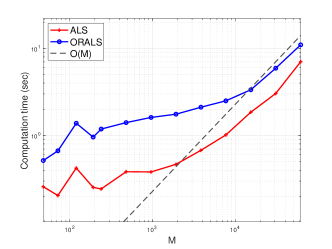
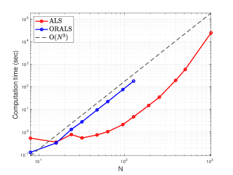
Figure 10: Computation time for the construction of the ALS and ORALS estimators, as a function of $M$ (left) and of $N$ (right). In both plots, the other parameters are set as: $L=2$, $d=1$, $n=8$; in the first plot $N=16$, and in the second plot $M=1024$; the interaction kernel is the inverse Fourier transform of a random vector with decaying coefficients, and no regularization is imposed. The scaling of ORALS as $N^{3}$ in the figure on the right, instead of the expected $N^{4}$, as the term $MLdN^{3}$ overcomes $N^{4}$ for the values of the parameters we have here; we could not perform runs with larger $N$ due to the significant memory that would have been required. Tests are run on a machine with 2 processors with 12 cores each, and $448$GB of RAM.

B.2 Regularization

Regularization is helpful to produce stable solutions when the matrix in the least squares of ALS or ORALS is ill-conditioned, and the data is noisy. We have tested five methods to solve the ill-posed linear equations: direct backslash (denoted by “NONE”), pseudo-inverse, minimal norm least squares (denoted by “lsqmininorm”), the Tikhonov regularization with Euclidean norm (denoted by “ID”), and the data-adaptive RKHS Tikhonov regularization (denoted by “RKHS”).

The data-adaptive RKHS Tikhonov regularization uses the norm of an RKHS adaptive to data and the basis functions of the kernel. In estimating the kernel coefficients in ALS, in addition to the regression matrix and vector, it uses the basis matrix $B$ with entries

$$B_{\psi}=\frac{1}{(N-1)NLM}\sum_{l=0}^{L-1}\sum_{m=1}^{M}\sum_{j\neq i}\langle{\psi_{k}(\mathbf{r}_{ij,t_{l}}^{m}),\psi_{l}(\mathbf{r}_{ij,t_{l}}^{m})}\rangle_{\mathbb{R}^{d}},\quad\mathbf{r}_{ij,t}=X^{j}_{t}-X^{i}_{t}.$$ (B.1)

where $\{\psi_{k}\}_{k=1}^{p}$ are the basis functions in the parametric form and recall that $\sum_{j\neq i}:=\sum_{i=1}^{N}\sum_{j=1,j\neq i}^{N}$. In ORALS for the estimation of $\widehat{z}_{i,M}$ in (2.3), we supply the DARTR with basis matrix $I_{N}\otimes B_{\psi}\in\mathbb{R}^{Np\times N{p}}$ with $B_{\psi}$ in (B.1), where $\otimes$ denotes the Kronecker product of matrices.

Figure 11 shows the errors of regularized estimators in 10 simulations of the Lennard-Jones model. The model parameters are $N=20$, $p=3$, $L=5$ and $d=2$. Here, the sample size $M=64$ is relatively small, so the regression matrices in ORALS tend to be deficient-ranked; in contrast, the regression matrices in ALS are well-conditioned. The results show that the minimal norm least squares and DARTR lead to more robust and accurate estimators than the other methods for the ORALS, but all methods perform similarly for ALS. Additional numerical tests show that as the sample size increases, the regression matrices for both ORALS and ALS become well-posed, and the direct backslash and the pseudo-inversion lead to accurate solutions robust to noise.

In short, regularization is helpful when the regression matrices are ill-conditioned and the data is noisy; otherwise, either the direct backslash or the pseudo-inversion is adequate. In the parametric estimation of the kernel, the regression matrices are often well-conditioned. However, in nonparametric estimation, the regression matrices are often ill-conditioned and even rank-deficient in the process of selecting an optimal dimension for the hypothesis space to achieve the bias-variance tradeoff.

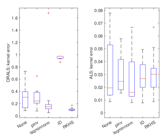
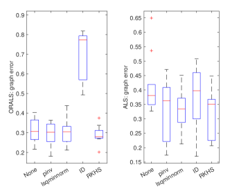
Figure 11: Errors of estimators in 10 simulations for different regularization methods. Here the regression matrices are deficient-ranked due to a small sample size $M=64$. The other parameters are $N=20$, $p=3$, $L=5$ and $d=2$.

Another type of regularization, different from those above that regularize the least squares in ALS or ORALS, is to enforce the low-rank property. Such regularizers include minimizing the nuclear norm [RFP10] or adding a term maintaining the norm-preserving property of the Hessian of the loss function [GJZ17]. They could be beneficial to the operation regression stage of the ORALS algorithm. We leave further exploration of these regularizers in future work.

B.3 Dependence on noise level and stochastic force

To examine robustness to stochastic force and observation noise, we test the error decay in the scale of the stochastic force and the noise level.

Figure 12 shows that for both ALS and ORALS estimators, the error decays linearly in the stochastic force level $\sigma$ in 100 simulations. In each simulation, we set observation noise with $\sigma_{obs}=10^{-7}$, the sample size $M=1000$. In particular, to see the effects of the stochastic force, we use long trajectories with time length $T=100$.

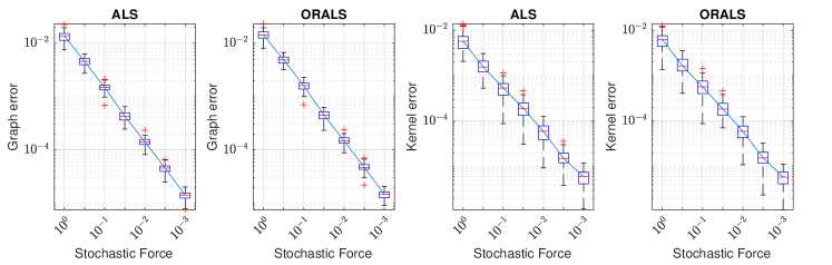
Figure 12: Decay of estimation error as the stochastic force decreases.

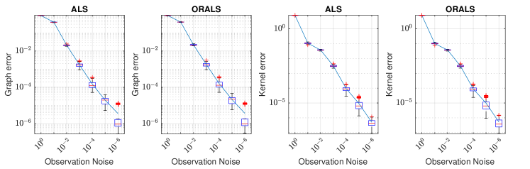
Figure 13: Decay of estimation error as the observation noise level decreases.

Similarly, Figure 13 shows that for both ALS and ORALS estimators, the error decays linearly in the noise level $\sigma_{obs}$ in 100 simulations. In each simulation, we take $\sigma=0$, $M=1000$, and $T=1$.

B.4 Additional tests on a directed graph on a circle

We also provide an example with a very simple graph in our admissible set $\mathcal{M}$, i.e., a directed circle graph. We present the graph, kernel estimation, and true trajectory in Figure 14; the rest of the results are very similar to the previous settings and are hence omitted.

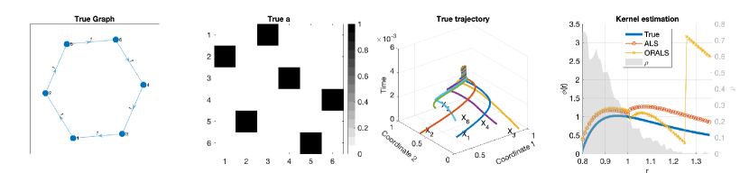
Figure 14: An example of the simplest graph, the true trajectory, and the kernel estimators. Each particle only follows one other particle, forming a spiral dynamical behavior. There is limited data of $r\in[1.2,1.4]$ since particles quickly converge together, leading to small values of $\rho$ in the region. As a result, the kernel estimators have large errors in the region; yet, their overall $L^{2}_{\rho}$ errors remain small with $\varepsilon_{K}$ for ALS is $1.19\times 10^{-2}$ and for ORALS is $1.89\times 10^{-2}$.

B.5 Additional details for identifying the leader-follower model

We examine a Leader-follower system where leaders have significant impacts on others; see the left panel of Figure 15. In the Impact-Influence coordinate, as shown in the middle panel of Figure 15, one can observe that the leaders $A1$ and $A6$ stand out from the rest. As the sample size $M$ increases, both the estimated graph $\widehat{\mathbf{a}}$ and the estimated interaction kernel $\widehat{\Phi}$ in the top of (6) become more precise. It becomes evident that a more accurate estimator $\widehat{\mathbf{a}}$ contributes to more precise identifications of leaders and their followers. The Leader-follower network estimated with $M=100$ almost recovers the true network (the left one in Figure 15). Thus, the clustering result of $M=100$ shown in the last row of the right panel in Figure 15 aligns with the ground truth depicted in the first row. Nevertheless, it’s noteworthy that identifying leaders and properly classifying followers remain feasible even when the estimator $\widehat{\mathbf{a}}$ is not highly precise.

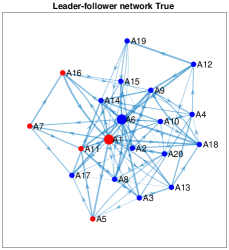
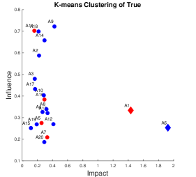
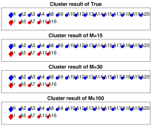
Figure 15: Left: the true Leader-follower network; Middle: the clustering of the true system, with two groups led by $A1$ (red group) and $A6$ (blue group); Right: the results of cluster based on the estimates with sample sizes $M\in\{15,30,100\}$. The graph errors (in Frobenius norm) are $0.1254$, $9.8\times 10^{-3}$, $1.8\times 10^{-3}$; and the kernel errors are $0.0115$, $1.4\times 10^{-3}$, $3\times 10^{-4}$.

Appendix C Connection with matrix sensing and RIP

In this section, we connect our joint inference problem with matrix sensing (see [GJZ17, ZSL19, RFP10] for example) and study the restricted isometry property (RIP) of the joint inference.

Matrix sensing and RIP.

The matrix sensing problem aims to find a low-rank matrix $Z^{*}\in\mathbb{R}^{n_{1}\times n_{2}}$ from data $b_{m}=\langle A_{m},Z^{*}\rangle_{F}$, where $A_{1},\cdots,A_{M}\in\mathbb{R}^{n_{1}\times n_{2}}$ are sensing matrices. To find $Z^{*}$ with rank $r\ll n_{1}\wedge n_{2}$, one solves the following non-convex optimization problem

$$\min_{Z\in\mathbb{R}^{n_{1}\times n_{2}},\text{rank}(Z)=r}F(Z)=\frac{1}{M}\sum_{m=1}^{M}|\langle A_{m},Z\rangle_{F}-b_{m}|^{2}=\frac{1}{M}\sum_{m=1}^{M}|\emph{Tr}(A_{m}^{\rm T}Z)-b_{m}|^{2}\,.$$ (C.1)

It is well-known that the constrained optimization problem (C.1) is NP-hard. A common method of factorization is introduced by Burer and Monteiro [BM03, BM05] to treat (C.1). Namely, we express $Z=UV^{\rm T}$ where $U\in\mathbb{R}^{n_{1}\times r}$ and $V\in\mathbb{R}^{n_{2}\times r}$. Then (C.1) can be transformed to an unconstraint problem

$$\min_{U\in\mathbb{R}^{n_{1}\times r},V\in\mathbb{R}^{n_{2}\times r}}F(U,V) =\frac{1}{M}\sum_{m=1}^{M}|\langle A_{m},UV^{\rm T}\rangle_{F}-b_{m}|^{2}$$ (C.2)

$$=\frac{1}{M}\sum_{m=1}^{M}|\emph{Tr}(A_{m}^{\rm T}UV^{\rm T})-b_{m}|^{2}=\frac{1}{M}\sum_{m=1}^{M}|\emph{Tr}(U^{\rm T}A_{m}V)-b_{m}|^{2}\,.$$

To simplify the notations, let us define a linear sensing operator $\mathscr{A}:\mathbb{R}^{n_{1}\times n_{2}}\to\mathbb{R}^{M}$ by

$$\mathscr{A}(Z)=\bigg{(}\frac{1}{\sqrt{M}}\langle A_{1},Z\rangle_{F},\cdots,\frac{1}{\sqrt{M}}\langle A_{M},Z\rangle_{F}\bigg{)}\,.$$ (C.3)

Definition C.1 (Restricted isometry property (RIP))

The linear map $\mathscr{A}$ satisfy the $(r,\delta_{r})$-RIP condition with the RIP constant $\delta=\delta_{r}\in[0,1)$ if there is a (strictly) positive constant $C$

$$(1-\delta)\left\|Z\right\|_{F}^{2}\leq\frac{1}{C}\left\|\mathscr{A}(Z)\right\|_{2}^{2}=\frac{1}{CM}\sum_{m=1}^{M}\langle A_{m},Z\rangle_{F}^{2}\leq(1+\delta)\left\|Z\right\|_{F}^{2}$$ (C.4)

holds for all $Z$ with rank at most $r$. We also simply say that $\mathscr{A}$ satisfies the rank-$r$ RIP condition without specifying the RIP constant $\delta_{r}\in[0,1)$.

Remark C.2

The normalization factor $C$ in the condition (C.4) was introduced in [RT11]. It enables the application of RIP to a larger class of sensing matrices that can be scaled to near isometry. In particular, in our setting, the sensing matrices are mostly far from an isometry.

Restricted isometry property and the restricted isometry constant are powerful tools in the theory of matrix sensing [RFP10], a generalization of compressed sensing [CT05]. For example, it can characterize the identifiability of matrix sensing problems.

Theorem C.3 (Theorem 3.2 in [RFP10])

Suppose that $\delta_{2r}<1$ for some integer $r\geq 1$, i.e., $\mathscr{A}$ satisfy the rank-$2r$ RIP condition for $r\geq 1$. Then $Z^{*}$ is the only matrix of rank at most $r$ satisfying $\mathscr{A}(Z)=b=[b_{1},\cdots,b_{M}]^{\rm T}$.

This article establishes a connection between the rank-1 and rank-2 Restricted Isometry Property (RIP) conditions and their counterparts in joint coercivity conditions.

Joint inference of $\mathbf{a}$ and $c$ as matrix sensing problems.

In our setting (1.1), the estimator $(\widehat{\mathbf{a}},\widehat{c})$ is the minimizer of the following loss function

$$\mathcal{E}_{L,M}(\mathbf{a},c) =\frac{1}{MT}\sum_{l=0,m=1}^{L-1,M}\left\|\Delta\mathbf{X}_{t_{l}}^{m}-\mathbf{a}\mathbf{B}(\mathbf{X}_{t_{l}}^{m})c\Delta t\right\|_{F}^{2}=\sum_{i=1}^{N}\mathcal{E}^{(i)}_{L,M}(\mathbf{a}_{i\cdot},c)$$

$$\text{where}\quad\mathcal{E}^{(i)}_{L,M}(\mathbf{a}_{i\cdot},c) =\frac{1}{MT}\sum_{l=0,m=1}^{L-1,M}\left\|(\Delta\mathbf{X}_{t_{l}}^{m})_{i}-\mathbf{a}_{i\cdot}\mathbf{B}(\mathbf{X}_{t_{l}}^{m})_{i}c\Delta t\right\|_{F}^{2}\,.$$ (C.5)

If we minimize the loss function $\mathcal{E}_{L,M}(\mathbf{a},c)$ row by row, i.e., by minimizing the loss functions $\mathcal{E}^{(i)}_{L,M}(\mathbf{a}_{i\cdot},c)$ for $i=1$ to $N$, each minimization is a rank-one matrix sensing problems (C.2) by substituting $U=\mathbf{a}_{i\cdot}$, $V=c$, $b_{m}=(\Delta\mathbf{X}_{t_{l}}^{m})_{i}$ and $A_{m}=\mathbf{B}(\mathbf{X}_{t_{l}}^{m})_{i}$ for each row $i$. To illustrate the idea, consider $d=1$, $L=1$, and $\Delta t=1$. Thus we set the rank-one decomposition $Z=UV^{\rm T}$ where $U=\mathbf{a}_{i\cdot}\in\mathbb{R}^{N-1}$ and $V=c\in\mathbb{R}^{p}$. Also, we define the sensing operator $\mathscr{A}:\mathbb{R}^{(N-1)\times p}\to\mathbb{R}^{M}$ with the sensing matrices

$$A_{m}=\mathbf{B}(\mathbf{X}_{t_{0}}^{m})_{i}=\Big{[}\psi_{k}\big{(}X_{t_{0}}^{j,m}-X_{t_{0}}^{i,m}\big{)}\Big{]}_{j\neq i\atop 1\leq k\leq p}\,,\quad m=1,\cdots,M\,,$$ (C.6)

where $\mathbf{X}_{t_{0}}=(X_{t_{0}}^{1},\cdots,X_{t_{0}}^{N})$ is the initial condition and $\{\psi_{k}\}_{k=1}^{p}$ represents the basis functions. Therefore,

$$\mathbf{a}_{i\cdot}\mathbf{B}(\mathbf{X}_{t_{0}}^{m})_{i}c=\langle A_{m},Z\rangle_{F}=\emph{Tr}(A_{m}^{\rm T}UV^{\rm T})\,.$$

In Section 4.3, we introduce a model (4.4) with $Q$ types of interaction kernels. We shall take $Q=2$ as an example to explain the connection with higher-rank matrix sensing problems. Namely, $\kappa(i)=1$ or $2$ indicating the type of kernel for agent $i$, and the coefficients are

$$c_{ki}=c_{k}^{\kappa(i)}:=\begin{cases}c_{k}^{(1)}\,,&\kappa(i)=1\,;\\ c_{k}^{(2)}\,,&\kappa(i)=2\,.\end{cases}$$

Without loss of generality, we still set $d=1$, $L=1$, and consider $i$-th row. Thus, the interacting part in the system (4.5) can be rewritten to be

$$\mathbf{a}_{i\cdot}\mathbf{B}(\mathbf{X}_{t}^{m})_{i}\mathbf{c}_{\cdot i} =\sum_{j\neq i}\mathbf{a}_{ij}\sum_{k=1}^{p}\psi_{k}(X^{j,m}_{t}-X^{j,m}_{t})c_{k}^{\kappa(i)}$$

$$=\sum_{j\neq i}\mathbf{a}_{ij}^{(1)}\sum_{k=1}^{p}\psi_{k}(X^{j,m}_{t}-X^{i,m}_{t})c_{k}^{(1)}+\sum_{j=2}^{N}\mathbf{a}_{ij}^{(2)}\sum_{k=1}^{p}\psi_{k}(X^{j,m}_{t}-X^{i,m}_{t})c_{k}^{(2)}$$ (C.7)

where $\mathbf{a}_{ij}^{(1)}=\mathbf{a}_{ij}$ if $\kappa(i)=1$, $\mathbf{a}_{ij}^{(1)}=0$ if $\kappa(i)=2$ and $\mathbf{a}_{ij}^{(2)}$ is defined similarly. So, selecting a rank-two decomposition $Z=UV^{\rm T}$ with

$$U=[\mathbf{a}_{i\cdot}^{(1)},\mathbf{a}_{i\cdot}^{(2)}]\in\mathbb{R}^{(N-1)\times 2}\quad\text{and}\quad V=[c^{(1)},c^{(2)}]\in\mathbb{R}^{p\times 2}$$

we get (C) can be repressed as

$$\mathbf{a}_{i\cdot}\mathbf{B}(\mathbf{X}_{t}^{m})_{i}\mathbf{c}_{\cdot i}=\langle A_{m},Z\rangle_{F}=\emph{Tr}(A_{m}^{\rm T}UV^{\rm T})\,.$$

Here, $A_{m}$ is the same sensing matrix defined in (C.9). Also, for another multitype kernel model where the type of interacting kernel depends on agent $j$

$$\mathbf{a}_{i\cdot}\mathbf{B}(\mathbf{X}_{t}^{m})_{i}\tilde{\mathbf{c}}_{\cdot j} =\sum_{j\neq i}\mathbf{a}_{ij}\sum_{k=1}^{p}\psi_{k}(X^{j,m}_{t}-X^{j,m}_{t})\tilde{c}_{k}^{\kappa(j)}\,,$$

we have the same expression with $\mathbf{a}_{ij}^{(1)}$ and $\mathbf{a}_{ij}^{(2)}$ adapted accordingly.

In the classical matrix sensing problem (refer to, for example, [BM03, RFP10, LS23]), the entries of the sensing matrix are i.i.d. standard Gaussian random variables. However, it is noteworthy that the entries of $A_{m}$ in (C.6) exhibit high correlation. This characteristic presents a challenge, preventing us from employing the “leave-one-out” tool, as successfully applied in [LS23, CLP22], to prove the convergence of the alternating least square algorithm.

RIP and joint coercivity conditions.

The lower bound of RIP is closely related to the joint coercivity conditions in Definition 2.2. In the following, we illustrate that rank-1 and rank-2 RIP conditions lead to the rank-1 and rank-2 joint coercivity conditions, respectively, when $\mathcal{H}$ is finite-dimensional.

Proposition C.4

Let $\mathcal{H}=\textrm{span}\{\psi_{k}\}_{k=1}^{p}$ with $\{\psi_{k}\}_{k=1}^{p}$ being orthonormal in $L^{2}_{\rho_{L}}$ for $p\geq 1$. Let $\mathscr{A}_{i}:\mathbb{R}^{(N-1)\times p}\to\mathbb{R}^{M}$ be (row-wise) linear sensing operators in (C.3) with sensing matrices in (C.6). Let $r\in\{1,2\}$. Suppose $\mathscr{A}_{i}$ satisfies the rank-r RIP condition with a constant $\delta$ for all $i\in[N]$ uniform for all $M\to\infty$. Then, the rank-r joint coercivity condition holds.

Proof. Without loss of generality, we set $i=1$ and $L=1$ and abbreviate $\mathscr{A}_{1}$ as $\mathscr{A}$. We consider the rank-1 case first. For all rank-1 matrices $Z=uv^{\rm T}$, it is equivalent to consider any $u=\mathbf{a}_{1\cdot}\in\mathcal{M}$ (defined in (1.2)) and any $v=c\in\mathbb{R}^{p}$. Then, substituting (C.6) into (C.4) and sending $M$ to infinity, we get the lower bound by the Law of large numbers that

$$\left\|\mathscr{A}(Z)\right\|_{2}^{2} =\mathbb{E}\bigg{[}\bigg{|}\sum_{j=2}^{N}\mathbf{a}_{1j}\Phi(X_{t_{0}}^{j+1}-X_{t_{0}}^{1})\bigg{|}^{2}\bigg{]}$$

$$\geq C(1-\delta)\left\|Z\right\|_{F}^{2}=C(1-\delta)|\mathbf{a}_{1\cdot}|^{2}\|c\|_{\ell^{2}}^{2}$$

$$=C(1-\delta)|\mathbf{a}_{1\cdot}|^{2}\|\Phi\|_{\rho}^{2}$$

for any $\Phi=\sum_{k}c_{k}\psi_{k}\in\mathcal{H}$. Thus, the coercivity constant in (2.9) is $c_{\mathcal{H}}=C(1-\delta)$ for a finite-dimensional hypothesis space, where $C$ is the normalization constant in the RIP condition when the kernel is represented on an orthonormal basis.

Next, we consider the rank-2 case. Recall that lower bound in rank-2 RIP condition implies that $\left\|\mathscr{A}(Z)\right\|_{2}^{2}\geq C(1-\delta)\left\|Z\right\|_{F}^{2}$ for all matrices with rank equal or less than two, i.e., $Z=u_{1}v_{1}^{\rm T}+u_{2}v_{2}^{\rm T}$ for all $u_{1},u_{2}\in\mathbb{R}^{N-1}$ and $v_{1},v_{2}\in\mathbb{R}^{p}$. We aim to show that

$$\mathbb{E}\bigg{[}\bigg{|}\sum_{j=2}^{N}[\mathbf{a}_{1j}^{(1)}\Phi_{1}(X_{t_{0}}^{j+1}-X_{t_{0}}^{1})+\mathbf{a}_{ij}^{(2)}\Phi_{2}(X_{t_{0}}^{j+1}-X_{t_{0}}^{1})]\bigg{|}^{2}\bigg{]}\geq c_{\mathcal{H}}[|\mathbf{a}_{i\cdot}^{(1)}|^{2}\|\Phi_{1}\|_{\rho_{L}}^{2}+|\mathbf{a}_{i\cdot}^{(2)}|^{2}\|\Phi_{2}\|_{\rho_{L}}^{2}]$$ (C.8)

with $c_{\mathcal{H}}=C(1-\delta)$ for all $\Phi_{1},\Phi_{2}\in\mathcal{H}$ being orthogonal and for all weight matrices $\mathbf{a}^{(1)},\mathbf{a}^{(2)}\in\mathcal{M}$. For any $\Phi_{1}=\sum_{k}c_{1,k}\psi_{k}\in\mathcal{H}$ and $\Phi_{2}=\sum_{k}c_{2,k}\psi_{k}\in\mathcal{H}$ being orthogonal to each other, we have $c_{1}\perp c_{2}$ and $\left\|\mathbf{a}_{1\cdot}^{(1)}c_{1}^{\rm T}+\mathbf{a}_{1\cdot}^{(2)}c_{2}^{\rm T}\right\|_{F}^{2}=|\mathbf{a}_{1\cdot}^{(1)}|^{2}|c_{1}|^{2}+|\mathbf{a}_{1\cdot}^{(2)}|^{2}|c_{2}|^{2}$. Thus, with $u_{1}=\mathbf{a}_{1\cdot}^{(1)}$, $u_{2}=\mathbf{a}_{1\cdot}^{(2)}$ and $v_{1}=c_{1}$, $v_{2}=c_{2}$, the lower bound of rank-2 RIP amounts to

$$\left\|\mathscr{A}(Z)\right\|_{2}^{2} =\mathbb{E}\bigg{[}\bigg{|}\sum_{j=2}^{N}[\mathbf{a}_{1j}^{(1)}\Phi_{1}(X_{t_{0}}^{j+1}-X_{t_{0}}^{1})+\mathbf{a}_{ij}^{(2)}\Phi_{2}(X_{t_{0}}^{j+1}-X_{t_{0}}^{1})]\bigg{|}^{2}\bigg{]}$$

$$\geq C(1-\delta)\left\|Z\right\|_{F}^{2}=C(1-\delta)\left\|\mathbf{a}_{1\cdot}^{(1)}c_{1}^{\rm T}+\mathbf{a}_{1\cdot}^{(2)}c_{2}^{\rm T}\right\|_{F}^{2}$$

$$=C(1-\delta)[|\mathbf{a}_{1\cdot}^{(1)}|^{2}|c_{1}|^{2}+|\mathbf{a}_{1\cdot}^{(2)}|^{2}|c_{2}|^{2}]$$

$$=C(1-\delta)[|\mathbf{a}_{i\cdot}^{(1)}|^{2}\|\Phi_{1}\|_{\rho_{L}}^{2}+|\mathbf{a}_{i\cdot}^{(2)}|^{2}\|\Phi_{2}\|_{\rho_{L}}^{2}]\,.$$

So, we get (C.8) and finish the proof.   

Large RIP constants and local minima in our setting.

The RIP constant $\delta$ plays a crucial role in characterizing the presence of spurious local minima and the convergence of search algorithms; see for example, [BR17, GJZ17, LS23, CLP22]. Notably, when the rank $r=1$ and in the symmetric setting $U=V$ in equation (C.2), a precise RIP threshold of $\delta=\frac{1}{2}$ serves to establish both necessary and sufficient conditions for the exact recovery of $U=V$ in the matrix sensing problem (C.2). For example, readers can find the interesting result in [ZSL19].

Theorem C.5 (Theorem 3 in [ZSL19])

Let the sensing operator $\mathscr{A}$ satisfy $(2,\delta)$-RIP condition and the loss function $F(U)=\|\mathscr{A}(UU^{\rm T}-Z^{*})\|^{2}$.

1. If $\delta<1/2$, then $F$ has no spurious local minima.

2. If $\delta\geq 1/2$, then there exists a counterexample admitting a spurious local minima.

However, the non-symmetric case introduces additional complexity, and achieving exact recovery with a sharp threshold for the RIP constant remains an open challenge. Noisy case is another open question, as mentioned in [ZSL19].

Our joint inference problem is in a noisy, non-symmetric setting. Thus, the sharp results on $\delta$ in [ZSL19] for the symmetric noiseless setting do not apply. Nevertheless, the RIP constant $\delta$ provides insights into our problem, specifically regarding the existence of local minima and the convergence of the ALS algorithm.

As an example, we consider an interacting particle system with $N=3$ particles in $\mathbb{R}^{d}$ with $d=1$ and $L=1$. We consider Gaussian i.i.d. initial conditions $\mathbf{X}_{t_{0}}=(X^{1},X^{2},X^{3})\overset{i.i.d.}{\sim}\mathcal{N}(0,I_{3})$. To make it easy to present the results, we only consider two basis functions $\{\psi_{1}(x),\psi_{2}(x)\}$. Thus, giving $M$ samples, the sensing matrices $\{A_{m}\}_{m=1}^{M}$ (C.6) are

$$A_{m}=\Big{[}\psi_{k}\big{(}X^{j+1,m}-X^{1,m}\big{)}\Big{]}_{1\leq j\leq 2\atop 1\leq k\leq 2}=\begin{bmatrix}\psi_{1}\big{(}X^{2,m}-X^{1,m}\big{)}&\psi_{2}\big{(}X^{2,m}-X^{1,m}\big{)}\\ \psi_{1}\big{(}X^{3,m}-X^{1,m}\big{)}&\psi_{2}\big{(}X^{3,m}-X^{1,m}\big{)}\end{bmatrix}\,,$$ (C.9)

and the sensing operator $\mathscr{A}$ is defined as in (C.3) correspondingly. Verifying Restricted Isometry Property (C.4) and finding the RIP constant $\delta$ for the operator $\mathscr{A}$ are NP-hard problems in general.

We shall numerically estimate the RIP constant $\delta$ for rank $r=1$ as follows. First, compute the RIP ratios:

$$R_{\ell}=\frac{\left\|\mathscr{A}(u_{0}^{\ell}(v_{0}^{\ell})^{\rm T})\right\|_{2}^{2}}{\left\|u_{0}^{\ell}(v_{0}^{\ell})^{\rm T}\right\|_{2}^{2}}=\frac{1}{M}\sum_{m=1}^{M}\left|(u_{0}^{\ell})^{\rm T}A_{m}v_{0}^{\ell}\right|^{2}\,,\quad\ell=1,\cdots,2000\,,$$

where $\{u_{0}^{\ell},v_{0}^{\ell}\}_{\ell=1}^{2000}$ are unit vectors randomly sampled in $\mathbb{R}^{2}$. Next, normalize the RIP ratios to be in $[0,2]$. We choose $C=\frac{\max(\{R_{\ell}\})+\min(\{R_{\ell}\})}{2}$ in (C.4) so that $\widetilde{R}_{\ell}=\frac{R_{\ell}}{C}\in[0,2]$ and the RIP constant is given by

$$\delta=\frac{\max(\{R_{\ell}\})-\min(\{R_{\ell}\})}{\max(\{R_{\ell}\})+\min(\{R_{\ell}\})}\in(0,1)\,.$$

To highlight the effects of the basis functions on the RIP constant, we choose three sets of basis functions listed in Table 5.

Figure 16 shows the distributions of the normalized RIP ratios for these three basis functions when $M=2000$. As a reference, we also present numerical tests of the RIP ratios for the classical Gaussian sensing operator, where the entries of $A_{m}$ are i.i.d. standard Gaussian random variables. For the case of the Gaussian sensing operator, the normalized RIP ratios are clustered in the interval $[1-\delta,1+\delta]$ with the computed values for $\delta$ being $0.0461$, $0.0399$, and $0.0534$; these values agree with the well-established result in [RFP10, LS23] that $\delta\to 0$ when $M$ turns to infinity. In contrast, the normalized RIP ratios for the IPS spread widely in $[0,2]$ for all three sets of basis functions, and their RIP constants are $0.4151$, $0.8937$, and $0.9462$, which are relatively large.

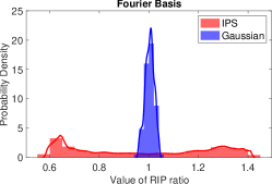
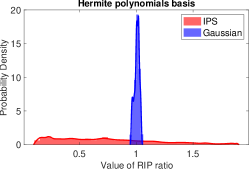
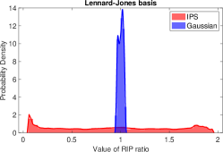
Figure 16: Distributions of the RIP ratios of the interacting particle system (IPS) in red color. The basis functions and the estimated RIP constants are in Table 5. The wide spread of the ratios in an interval $[1-\delta,1-\delta]$ indicates a large RIP constant $\delta$, particularly in the middle and right figures. As a reference, we also present distributions of the RIP ratios for the Gaussian sensing operator in blue color, for which the RIP constants, from left to right, are $0.0418$, $0.0456$, and $0.0474$.

	Left	Middle	Right
$\psi_{1}(x)$	$\sin(x)$	$x^{4}-6x^{2}+3$	$x^{-9}\mathbbm{1}_{[0.75,+\infty]}$
$\psi_{2}(x)$	$\cos(x)$	$x^{5}-10x^{3}+15x$	$x^{-3}\mathbbm{1}_{[0.25,+\infty]}$
RIP constant	0.4151	0.8937	0.9462

Table 5: The basis functions and the testing RIP constants in Figure 16. Left: Fourier basis; middle: Hermite polynomials basis; right: as in Section 3 for the Lennard-Jones interaction kernel.

A large RIP value indicates that the matrix sensing problem may involve local minima, as highlighted by Theorem C.5 and supported by findings in nonsymmetric scenarios in [BR17, GJZ17]. Therefore, local minima may exist in the joint inference, and we provide explicit examples. Let $U=\mathbf{a}_{1\cdot}=(u_{1},u_{2})\in\mathbb{R}^{2}$ and $V=c=(v_{1},v_{2})\in\mathbb{R}^{2}$ be unit vectors. We then have

$$(u_{1},u_{2})=(\cos(\theta_{1}),\sin(\theta_{1}))\,,\quad(v_{1},v_{2})=(\cos(\theta_{2}),\sin(\theta_{2}))\,,\quad\theta_{1},\theta_{2}\in[0,2\pi)\,,$$

and the ground truth $(U^{*},V^{*})$ with $U^{*}=(u_{1}^{*},u_{2}^{*})=(\cos(\theta_{1}^{*}),\sin(\theta_{1}^{*}))$ and $V^{*}=(v_{1}^{*},v_{2}^{*})=(\cos(\theta_{2}^{*}),\sin(\theta_{2}^{*}))$. The loss function denoted by $\mathcal{E}_{M}(U,V)$ depends on $\theta_{1}$ and $\theta_{2}$:

$$\mathcal{E}_{M}(\theta_{1},\theta_{2})=\mathcal{E}_{M}(U,V)=\frac{1}{M}\sum_{m=1}^{M}\big{|}(U^{*})^{\rm T}A_{m}V^{*}-U^{\rm T}A_{m}V\big{|}^{2}$$ (C.10)

where the sensing matrices $\{A_{m}\}$ are defined in (C.9) with basis functions listed in Table 5. It is clear that $(-U^{*},-V^{*})$ forms another global minimum pair, resulting in the loss function $\mathcal{E}_{M}$ being zero. The corresponding angles are referred to as $(\widetilde{\theta}_{1}^{*},\widetilde{\theta}_{2}^{*})$.

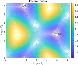
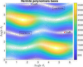
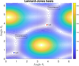
Figure 17: Contour plots of the loss functions for the three sets of basis functions. Local minima are present in the right two plots.

In Figure 17, the red and blue dots locate the ground truths $(\theta_{1}^{*},\theta_{2}^{*})$ and $(\widetilde{\theta}_{1}^{*},\widetilde{\theta}_{2}^{*})$, respectively. Text boxes label the local minima. The basis functions are set as Hermite polynomials basis in the middle panel Figure 17 and are set as basis for the Lennard-Jones interaction kernel in the right panel of Figure 17. The corresponding error functions $\mathcal{E}_{M}(\theta_{1},\theta_{2})$ are plotted with $M=100$ samples and random choices of ground truth. Upon conducting a limited number of tests, the presence of local minima is not rare to be observed, even posing normalization constraints on $U$ and $V$. This observation is expected, given that both scenarios exhibit high RIP constants, as illustrated in Table 5. However, we never witness the existence of local minima with the selection of Fourier basis $\{\psi_{1}(x)=\sin(x),\psi_{2}(x)=\cos(x)\}$; see an example of the error function with $M=200$ samples in the left panel of Figure 17. This is kind of surprising, as conventional wisdom suggests that the RIP value of the nonsymmetric case should be half that of the symmetric case to ensure the absence of spurious local minima phenomena, as discussed in, for instance, [GJZ17]. The disappearance of local minima of the error function $\mathcal{E}_{M}(\theta_{1},\theta_{2})=\mathcal{E}_{M}(U,V)$ may be due to the constraints that $U$ and $V$ are unit vectors. Investigating the sharpness of the Restricted Isometry Property (RIP), exploring the non-existence of local minima, and understanding the convergence of the ALS algorithm for the joint inference in interacting particle systems on graphs are key subjects for future research.

Appendix D Algorithm: Three-fold ALS

The three-fold ALS algorithm finds the minimizers of the loss function:

$$(\widehat{\mathbf{a}},\widehat{\textbf{u}},\widehat{\textbf{v}}) =\underset{\begin{subarray}{c}(\mathbf{a},\textbf{u},\textbf{v})\in\mathcal{M}\times\mathbb{R}^{p\times Q}\times\mathbb{R}^{N\times Q}\\ \textbf{v}^{\rm T}\textbf{v}=I_{Q}\end{subarray}}{\operatorname{arg}\operatorname{min}}\;\mathcal{E}_{L,M}(\mathbf{a},\textbf{u},\textbf{v}),\,\,\,\text{ with}$$ (D.1)

$$\mathcal{E}_{L,M}(\mathbf{a},\textbf{u},\textbf{v}) :=\frac{1}{MT}\sum_{l=1,m=1}^{L,M}\left\|\Delta\mathbf{X}_{t_{l}}^{m}-\mathbf{a}\mathbf{B}(\mathbf{X}_{t_{l}}^{m})\textbf{u}\textbf{v}^{\rm T}\Delta t\right\|_{F}^{2},$$

with an additional condition that $\mathbf{c}=\textbf{u}\textbf{v}^{\rm T}$ has only $Q$ distinct columns.

Notice that the loss function (D.1) is quadratic in each of the unknowns $\mathbf{a},\textbf{u},\textbf{v}$ if we fix the other two. Thus, we can apply ALS to alternatively solve for each of the unknowns while fixing the other two, and we call this algorithm three-fold ALS. In each iteration, this algorithm proceeds with the following three steps. To ensure that $\mathbf{c}$ has only $Q$ distinct columns, we add an optional step of $K$-means.

Step 1: Inference of the weight matrix $\mathbf{a}$. Given a coefficient matrix u and a type matrix v, we estimate the weight matrix $\mathbf{a}$ from data by least squares. For every $i\in[N]$, with $\textbf{u},\textbf{v}$ fixed we obtain the minimizer of the loss function $\mathcal{E}_{L,M}(\mathbf{a},\textbf{u},\textbf{v})$ in (4.8) by solving $\nabla_{\mathbf{a}_{i\cdot}}\mathcal{E}_{L,M}(\mathbf{a},\textbf{u},\textbf{v})=0$, which is a linear equation in $\mathbf{a}_{i\cdot}$:

$$\widehat{\mathbf{a}}_{i\cdot}\mathcal{A}^{\textrm{ALS}}_{\textbf{u},\textbf{v},M,i}:=\widehat{\mathbf{a}}_{i\cdot}([\mathbf{B}(\mathbf{X}_{t_{l}}^{m})_{i}]_{l,m}\textbf{u}\textbf{v}_{i\cdot}^{\rm T})=[(\Delta\mathbf{X}_{t_{l}})_{i}]_{l,m}/\Delta t\,\ \ ,$$ (D.2)

using least squares with nonnegative constraints. The solution is then row-normalized to obtain an estimator $\widehat{\mathbf{a}}_{i,\cdot}$ in the admissible set.

Step 2: Inference of the coefficient matrix u. Next, we estimate the coefficient matrix u by minimizing the loss function $\mathcal{E}_{L,M}(\mathbf{a},\textbf{u},\textbf{v})$ in (4.8) with the (estimated) weight matrix $\mathbf{a}$ and a type matrix v. The minimizer is a solution to

$$\mathbf{a}_{i\cdot}[\mathbf{B}(\mathbf{X}_{t_{l}}^{m})_{i}]_{l,m}\widehat{\textbf{u}}\textbf{v}_{i\cdot}^{\rm T}=[\Delta\mathbf{X}^{i}_{t_{l}}]_{l,m}/\Delta t,\quad i\in[N].$$ (D.3)

Noting that for each $i\in[N]$,

$$\langle{\mathcal{A}^{\textrm{ALS}}_{\mathbf{a},\textbf{v},M,i},\widehat{\textbf{u}}}\rangle_{F}:=\langle{\mathbf{a}_{i\cdot}[\mathbf{B}(\mathbf{X}_{t_{l}}^{m})_{i}]_{l,m}^{\rm T}\otimes\textbf{v}_{i,\cdot},\widehat{\textbf{u}}}\rangle_{F}=\mathbf{a}_{i\cdot}[\mathbf{B}(\mathbf{X}_{t_{l}}^{m})_{i}]_{l,m}\widehat{\textbf{u}}\textbf{v}_{i\cdot}^{\rm T},$$

we can write a linear equation for $\widehat{\textbf{u}}$ using Frobenius inner product:

$$\mathcal{A}_{\mathbf{a},\textbf{v},M}^{\textrm{ALS}}\widehat{\textbf{u}}:=\left(\langle{\mathcal{A}^{\textrm{ALS}}_{\mathbf{a},\textbf{v},M,i},\widehat{\textbf{u}}}\rangle_{F}\right)_{i}=[\Delta\mathbf{X}_{t_{l}}]_{l,m}/\Delta t.$$ (D.4)

Step 3: Inference of the type matrix v. At last, we estimate the type matrix v by minimizing the loss function $\mathcal{E}_{L,M}(\mathbf{a},\textbf{u},\textbf{v})$ in (4.8) with the (estimated) weight matrix $\mathbf{a}$ and coefficient matrix u. Firstly we solve the linear equation,

$$\mathcal{A}^{\textrm{ALS}}_{\mathbf{a},\textbf{u},M,i}\widehat{\textbf{v}}_{i\cdot}^{\rm T}:=(\mathbf{a}_{i\cdot}[\mathbf{B}(\mathbf{X}_{t_{l}}^{m})_{i}]_{l,m}\textbf{u})\widehat{\textbf{v}}_{i\cdot}^{\rm T}=[(\Delta\mathbf{X}_{t_{l}})_{i}]_{l,m}/\Delta t\,,\quad i\in[N]$$ (D.5)

with the result denoted as $\widehat{\textbf{v}}^{\prime}$. Then, we apply a final normalization step to ensure the orthogonality at the end. Namely, we find an orthogonal matrix $\widehat{\textbf{v}}$ such that

$$\widehat{\textbf{v}}=\underset{\textbf{v}^{\rm T}\textbf{v}=I_{Q}}{\operatorname{arg}\operatorname{min}}\;\left\|\textbf{v}-\widehat{\textbf{v}}^{\prime}\right\|_{F}.$$ (D.6)

The above problem is known as the orthogonal Procrustes problem [GD04], and the solution is given by normalizing the singular values of $\widehat{\textbf{v}}^{\prime}$, namely,

$$\widehat{\textbf{v}^{\prime}}=U\Sigma V^{\rm T}\implies\widehat{\textbf{v}}=UV^{\rm T}.$$ (D.7)

Step 4 (optional): apply $K$-means to the estimated $\widehat{\textbf{v}}$. To enforce the coefficient matrix $\mathbf{c}$ to have $Q$ distinct columns, we cluster the rows of $\widehat{\textbf{v}}$ by $K$-means.

Algorithm 3 summarizes the above iterative procedure.

Algorithm 3 Three-fold ALS

procedure Three-fold ALS($\{\mathbf{X}^{m}_{t_{0}:t_{L}}\}_{m=1}^{M},\{\psi_{k}\}_{k=1}^{p},\epsilon,{p}_{maxiter}$)

    Construct the arrays $\{\mathbf{B}(\mathbf{X}_{t_{l}}^{m})\}_{l,m}$ and $\{\Delta\mathbf{X}_{t_{l}}^{m}\}$ in (1.5) for each trajectory.

    Randomly pick initial conditions $\widehat{\textbf{u}}_{0}$ and $\widehat{\textbf{v}}_{0}$.

    for $\tau=1,\dots,{p}_{maxiter}$ do

         Estimate the weight matrix $\widehat{\mathbf{a}}_{\tau}$ by solving (D.2) with $\textbf{u}=\widehat{\textbf{u}}_{\tau-1}$ and $\textbf{v}=\widehat{\textbf{v}}_{\tau-1}$, with nonnegative  least squares followed by a row normalization.

         Estimate the coefficient matrix $\widehat{\textbf{u}}_{\tau}$ by solving (D.4) with $\mathbf{a}=\widehat{\mathbf{a}}_{\tau}$ and $\mathbf{v}=\widehat{\mathbf{v}}_{\tau-1}$ by least squares.

         Estimate the type matrix $\widehat{\textbf{v}}_{\tau}$ by solving (D.5) with $\mathbf{a}=\widehat{\mathbf{a}}_{\tau}$ and $\mathbf{u}=\widehat{\mathbf{u}}_{\tau}$ by least squares followed  by normalization in singular values as in (D.7) and an optional step clustering the rows of $\widehat{\textbf{v}}$.

         Exit loop if $||\widehat{\mathbf{a}}_{\tau}-\widehat{\mathbf{a}}_{\tau-1}||\leq\epsilon||\widehat{\mathbf{a}}_{\tau-1}||$, $||\widehat{\textbf{u}}_{\tau}-\widehat{\textbf{u}}_{\tau-1}||\leq\epsilon||\widehat{\textbf{u}}_{\tau-1}\|$ and $||\widehat{\textbf{v}}_{\tau}-\widehat{\textbf{v}}_{\tau-1}||\leq\epsilon||\widehat{\textbf{v}}_{\tau-1}\|$.     return $\widehat{\mathbf{a}}_{\tau},\widehat{\textbf{u}}_{\tau},\widehat{\textbf{v}}_{\tau}$.

Acknowledgement

This work was supported by National Science Foundation Grants DMS-DMS-2238486; Air Force Office of Scientific Research Grant AFOSR-FA9550-20-1-0288, FA9550-21-1-0317, and FA9550-23-1-0445; and the Johns Hopkins Catalyst Award.

References

- [ABK+23] Pedro Abdalla, Afonso S. Bandeira, Martin Kassabov, Victor Souza, Steven H. Strogatz, and Alex Townsend. Expander graphs are globally synchronizing, 2023.
- [ASM22] Arash Amini, Qiyu Sun, and Nader Motee. Learning nonlinear couplings in swarm of agents from a single sample trajectory. In 2022 IEEE 61st Conference on Decision and Control (CDC), pages 168–173, 2022.
- [BFHM16] Mattia Bongini, Massimo Fornasier, M. Hansen, and Mauro Maggioni. Inferring interaction rules from observations of evolutive systems i: The variational approach, 2016.
- [Bis06] Christopher M. Bishop. Pattern recognition and machine learning. Information Science and Statistics. Springer, New York, 2006.
- [BLM+06] Stefano Boccaletti, Vito Latora, Yamir Moreno, Martin Chavez, and D-U Hwang. Complex networks: Structure and dynamics. Physics reports, 424(4-5):175–308, 2006.
- [BM03] Samuel Burer and Renato DC Monteiro. A nonlinear programming algorithm for solving semidefinite programs via low-rank factorization. Mathematical Programming, 95(2):329–357, 2003.
- [BM05] Samuel Burer and Renato D. C. Monteiro. Local minima and convergence in low-rank semidefinite programming. Math. Program., 103(3):427–444, 2005.
- [BR17] Sohail Bahmani and Justin Romberg. Phase Retrieval Meets Statistical Learning Theory: A Flexible Convex Relaxation. In Aarti Singh and Jerry Zhu, editors, Proceedings of the 20th International Conference on Artificial Intelligence and Statistics, volume 54 of Proceedings of Machine Learning Research, pages 252–260. PMLR, 20–22 Apr 2017.
- [Can08] Emmanuel J. Candès. The restricted isometry property and its implications for compressed sensing. C. R. Math. Acad. Sci. Paris, 346(9-10):589–592, 2008.
- [CK22] Sui Tang Christian Kümmerle, Mauro Maggioni. Learning transition operators from sparse space-time samples. submitted, 2022.
- [CLP22] Kabir Aladin Chandrasekher, Mengqi Lou, and Ashwin Pananjady. Alternating minimization for generalized rank one matrix sensing: Sharp predictions from a random initialization. 2022.
- [CR09] Emmanuel J. Candès and Benjamin Recht. Exact matrix completion via convex optimization. Found. Comput. Math., 9(6):717–772, 2009.
- [CS02] Felipe Cucker and Steve Smale. Best Choices for Regularization Parameters in Learning Theory: On the Bias—Variance Problem. Found. Comput. Math., 2(4):413–428, 2002.
- [CT05] Emmanuel J. Candès and Terence Tao. Decoding by linear programming. IEEE Trans. Inform. Theory, 51(12):4203–4215, 2005.
- [CT10] Emmanuel J. Candès and Terence Tao. The power of convex relaxation: near-optimal matrix completion. IEEE Trans. Inform. Theory, 56(5):2053–2080, 2010.
- [DB14] Florian Dörfler and Francesco Bullo. Synchronization in complex networks of phase oscillators: A survey. Automatica, 50(6):1539–1564, 2014.
- [DTW18] Yixuan Ding, Cheng Tan, and Shing Wong Wing. Discrete-time Hegselmann-Krause model for a leader-follower social network. In 2018 37th Chinese Control Conference (CCC), pages 9692–9697. IEEE, 2018.
- [EHN96] Heinz Werner Engl, Martin Hanke, and Andreas Neubauer. Regularization of inverse problems, volume 375. Springer Science & Business Media, 1996.
- [FMMZ22] Jinchao Feng, Mauro Maggioni, Patrick Martin, and Ming Zhong. Learning interaction variables and kernels from observations of agent-based systems. Proc. IFAC 2022, 2022.
- [GD04] John C Gower and Garmt B Dijksterhuis. Procrustes problems, volume 30. OUP Oxford, 2004.
- [GFR+22] Dibakar Ghosh, Mattia Frasca, Alessandro Rizzo, Soumen Majhi, Sarbendu Rakshit, Karin Alfaro-Bittner, and Stefano Boccaletti. The synchronized dynamics of time-varying networks. Physics Reports, 949:1–63, 2022.
- [GHN19] Silvia Gazzola, Per Christian Hansen, and James G Nagy. Ir tools: a matlab package of iterative regularization methods and large-scale test problems. Numerical Algorithms, 81(3):773–811, 2019.
- [GJZ17] Rong Ge, Chi Jin, and Yi Zheng. No spurious local minima in nonconvex low rank problems: A unified geometric analysis. In International Conference on Machine Learning, pages 1233–1242. PMLR, 2017.
- [Han98] Per Christian Hansen. Rank-deficient and discrete ill-posed problems: numerical aspects of linear inversion. SIAM, 1998.
- [HZBL+20] Jalil Hasanyan, Lorenzo Zino, Daniel Alberto Burbano Lombana, Alessandro Rizzo, and Maurizio Porfiri. Leader–follower consensus on activity-driven networks. Proceedings of the Royal Society A, 476(2233):20190485, 2020.
- [Kal05] Olav Kallenberg. Probabilistic symmetries and invariance principles. Probability and its Applications (New York). Springer, New York, 2005.
- [KDL80] P.M. Kroonenberg and J. De Leeuw. Principal components analysis of three-mode data by means of alternating least squares algorithms. Psychometrika, 45:69–97, 1980.
- [Kur75] Yoshiki Kuramoto. Self-entrainment of a population of coupled non-linear oscillators. In International Symposium on Mathematical Problems in Theoretical Physics: January 23–29, 1975, Kyoto University, Kyoto/Japan, pages 420–422. Springer, 1975.
- [Lax02] Peter D. Lax. Functional analysis. Pure and Applied Mathematics (New York). Wiley-Interscience [John Wiley & Sons], New York, 2002.
- [LH95] Charles L Lawson and Richard J Hanson. Solving least squares problems. SIAM, 1995.
- [LLA22] Fei Lu, Quanjun Lang, and Qingci An. Data adaptive RKHS Tikhonov regularization for learning kernels in operators. Proceedings of Mathematical and Scientific Machine Learning, PMLR 190:158-172, 2022.
- [LLM+21] Zhongyang Li, Fei Lu, Mauro Maggioni, Sui Tang, and Cheng Zhang. On the identifiability of interaction functions in systems of interacting particles. Stochastic Processes and their Applications, 132:135–163, 2021.
- [LMT21a] Fei Lu, Mauro Maggioni, and Sui Tang. Learning interaction kernels in heterogeneous systems of agents from multiple trajectories. Journal of Machine Learning Research, 22(32):1–67, 2021.
- [LMT21b] Fei Lu, Mauro Maggioni, and Sui Tang. Learning interaction kernels in stochastic systems of interacting particles from multiple trajectories. Foundations of Computational Mathematics, pages 1–55, 2021.
- [LRW23] Daniel Lacker, Kavita Ramanan, and Ruoyu Wu. Local weak convergence for sparse networks of interacting processes. Ann. Appl. Probab., 33(2):643–688, 2023.
- [LS23] Kiryung Lee and Dominik Stöger. Randomly initialized alternating least squares: fast convergence for matrix sensing. SIAM J. Math. Data Sci., 5(3):774–799, 2023.
- [LZTM19] Fei Lu, Ming Zhong, Sui Tang, and Mauro Maggioni. Nonparametric inference of interaction laws in systems of agents from trajectory data. Proc. Natl. Acad. Sci. USA, 116(29):14424–14433, 2019.
- [MT14] Sebastien Motsch and Eitan Tadmor. Heterophilious Dynamics Enhances Consensus. SIAM Rev, 56(4):577 – 621, 2014.
- [MTZM23] Jason Miller, Sui Tang, Ming Zhong, and Mauro Maggioni. Learning theory for inferring interaction kernels in second-order interacting agent systems. Sampling Theory, Signal Processing, and Data Analysis, 21(1):21, 2023.
- [NÁBV10] Máté Nagy, Zsuzsa Ákos, Dora Biro, and Tamás Vicsek. Hierarchical group dynamics in pigeon flocks. Nature, 464(7290):890–893, 2010.
- [OSFM07] Reza Olfati-Saber, J Alex Fax, and Richard M Murray. Consensus and cooperation in networked multi-agent systems. Proceedings of the IEEE, 95(1):215–233, 2007.
- [PM21] E Pesce and G Montana. Learning multi-agent coordination through graph-driven communication. In 2021 International Conference on Autonomous Agents and MultiAgent Systems, pages 964–973, 2021.
- [RFP10] Benjamin Recht, Maryam Fazel, and Pablo A Parrilo. Guaranteed minimum-rank solutions of linear matrix equations via nuclear norm minimization. SIAM review, 52(3):471–501, 2010.
- [RT11] Angelika Rohde and Alexandre B. Tsybakov. Estimation of high-dimensional low-rank matrices. Ann. Statist., 39(2):887–930, 2011.
- [TJP03] Herbert G Tanner, Ali Jadbabaie, and George J Pappas. Stable flocking of mobile agents, part i: Fixed topology. In 42nd IEEE International Conference on Decision and Control (IEEE Cat. No. 03CH37475), volume 2, pages 2010–2015. IEEE, 2003.
- [Tro12] Joel A. Tropp. User-friendly tail bounds for sums of random matrices. Found. Comput. Math., 12(4):389–434, 2012.
- [WPC+20] Zonghan Wu, Shirui Pan, Fengwen Chen, Guodong Long, Chengqi Zhang, and S Yu Philip. A comprehensive survey on graph neural networks. IEEE transactions on neural networks and learning systems, 32(1):4–24, 2020.
- [WS06] Wei Wang and J-JE Slotine. A theoretical study of different leader roles in networks. IEEE Transactions on Automatic Control, 51(7):1156–1161, 2006.
- [WSL23] Xiong Wang, Inbar Seroussi, and Fei Lu. Optimal minimax rate of learning interaction kernels. arXiv preprint arXiv:2311.16852, 2023.
- [ZSL19] Richard Y Zhang, Somayeh Sojoudi, and Javad Lavaei. Sharp restricted isometry bounds for the inexistence of spurious local minima in nonconvex matrix recovery. J. Mach. Learn. Res., 20(114):1–34, 2019.