The baryon cycle in modern cosmological hydrodynamical simulations

Abstract

In recent years, cosmological hydrodynamical simulations have proven their utility as key interpretative tools in the study of galaxy formation and evolution. In this work, we present a like-for-like comparison between the baryon cycle in three publicly available, leading cosmological simulation suites: EAGLE, IllustrisTNG, and SIMBA. While these simulations broadly agree in terms of their predictions for the stellar mass content and star formation rates of galaxies at $z\approx 0$, they achieve this result for markedly different reasons. In EAGLE and SIMBA, we demonstrate that at low halo masses ($M_{\rm 200c}\lesssim 10^{11.5}\,M_{\odot}$), stellar feedback (SF)-driven outflows can reach far beyond the scale of the halo, extending up to $2-3\times R_{\rm 200c}$. In contrast, in TNG, SF-driven outflows, while stronger at the scale of the ISM, recycle within the CGM (within $R_{\rm 200c}$). We find that AGN-driven outflows in SIMBA are notably potent, reaching several times $R_{\rm 200c}$ even at halo masses up to $M_{\rm 200c}\approx 10^{13.5}\,M_{\odot}$. In both TNG and EAGLE, AGN feedback can eject gas beyond $R_{\rm 200c}$ at this mass scale, but seldom beyond $2-3\times R_{\rm 200c}$. We find that the scale of feedback-driven outflows can be directly linked with the prevention of cosmological inflow, as well as the total baryon fraction of haloes within $R_{\rm 200c}$. This work lays the foundation to develop targeted observational tests that can discriminate between feedback scenarios, and inform sub-grid feedback models in the next generation of simulations.

1 Introduction

The baryon cycle represents a complex and interconnected set of processes, including gas accretion, star formation, chemical enrichment, and large scale outflows, that collectively drive the formation and evolution of galaxies (e.g., Oppenheimer & Davé 2006; Ford et al. 2014; Somerville & Davé 2015; Tumlinson et al. 2017; Anglés-Alcázar et al. 2017b; Oppenheimer et al. 2018). The interplay of these processes establishes a causal link between different scales: the interstellar medium (ISM), circum-galactic medium (CGM), and intergalactic medium (IGM); as well as a connection between the different baryonic components involved at each of these scales: stars, gas, and black holes.

The cosmological inflow of gas from the IGM, through the CGM, and eventually into the ISM provides the requisite fuel for the process of star formation (Kereš et al. 2005; Sánchez Almeida et al. 2014). Star formation occurs within the dense regions of the ISM, where efficient cooling and gravitational collapse leads to the initiation of nuclear fusion and the consequent birth of new stars (e.g. Kennicutt 1983; McKee & Ostriker 2007; Kennicutt & Evans 2012). A fraction of the gas that makes it into galaxy nuclei can also be accreted onto supermassive black holes (SMBH), which are known to inhabit the dense central regions of many galaxies (see reviews by Ferrarese & Ford 2005; Kormendy & Ho 2013; Heckman & Best 2014).

Both star formation and accretion onto SMBH drive large scale outflows, which play a crucial role in regulating the baryon cycle (Veilleux et al. 2005, 2020). Stellar feedback, through supernovae explosions, radiation, and stellar winds, injects energy, momentum, and enriched material into the ISM and potentially beyond (Heckman et al., 2015). Active galactic nucleus (AGN) feedback, powered by accretion onto supermassive black holes at galactic centers, also releases substantial amounts of energy and momentum, that can drive powerful outflows, impacting the surrounding gas and quenching star formation in some cases (e.g. Fabian 2012; Heckman & Best 2014; King & Pounds 2015).

On the scale of the ISM, various observational techniques provide relatively well-constrained measurements of the stellar mass, galaxy cold gas (${\rm H}$i and ${\rm H}_{2}$) content, and star formation rates. Beyond the ISM, direct observational constraints on the CGM and IGM gas are associated with increasing uncertainty due to its diffuse nature (e.g. Werk et al. 2014; Tumlinson et al. 2017). Outside the Milky Way, gas accretion has been detected in a number of cases where absorption signatures are identified in galaxy spectra (e.g. Rubin et al. 2012; Martin et al. 2012; Stone et al. 2016; for a review see Rubin 2017); and in a number of studies where it is possible to use a fortuitously-aligned background quasar to probe circumgalactic gas flows (e.g. Lehner et al. 2013; Bouché et al. 2016; Martin et al. 2019). Even with these discoveries, the rate at which the gas accretes and its associated properties have yet to be well-quantified on a statistical basis; and are associated with considerable uncertainties.

There is a significant body of literature presenting supporting evidence for the presence of feedback-driven gas outflows from galaxies (e.g., Heckman et al. 2000; Martin 2005; Veilleux et al. 2005; Feruglio et al. 2010; Newman et al. 2012; Rubin et al. 2014; Heckman et al. 2015; Schroetter et al. 2016; Chisholm et al. 2016; Rupke et al. 2019; for a recent review see Veilleux et al. 2020). However, in each case, the determination of associated mass flux is affected by several systematic uncertainties. In particular, a given outflow tracer only provides information about gas on a subset of spatial scales (nominally confined to well within a given halo virial radius), and to specific gas phases. Furthermore, these measurements are biased towards gas rich galaxies exhibiting particularly strong outflows – either those at high redshift, or local galaxies experiencing a starburst.

Modern cosmological hydrodynamical simulations constitute a powerful tool to explore the role of different processes within the baryon cycle, and galaxy evolution more broadly (e.g. Schaye et al. 2010; Dubois et al. 2014; Vogelsberger et al. 2014; Christensen et al. 2016; Schaye et al. 2015; Pillepich et al. 2018; Hopkins et al. 2018; Davé et al. 2019). However, in order to accurately simulate the formation of galaxy populations within the context of large-scale structure, it is crucial to model essential small-scale processes taking place within individual galaxies. These processes, such as star formation, black hole formation and accretion, and stellar and AGN feedback, operate at scales below the resolution capabilities of the simulations. Therefore, they are commonly incorporated using "sub-grid" techniques, which effectively account for their influence on galaxy evolution in a physically-motivated, but necessarily coarse-grained manner (for reviews, see Somerville & Davé 2015; Vogelsberger et al. 2020). A wide range of sub-grid techniques have demonstrated success in reproducing realistic galaxy populations in cosmological simulations, particularly in capturing the observed shape of the stellar mass function (e.g. Thorne et al. 2021; Schaye et al. 2023, see also §3).

Despite these promising results, recent studies have suggested that the behavior of the gaseous phase and the broader-scale baryon cycle differ significantly between different simulations and feedback models, and can be degenerate in producing the same stellar mass assembly in galaxies over cosmic time (Naab & Ostriker, 2017; Mitchell et al., 2018, 2020; Pandya et al., 2020; Davé et al., 2020; Villaescusa-Navarro et al., 2021; Ni et al., 2023; Tillman et al., 2023a). For example, Davé et al. (2020) compare the cool gas content of galaxies in three publicly available modern cosmological hydrodynamical simulations – EAGLE, TNG100, and SIMBA (for a technical overview of the sub-grid prescriptions in each simulation, see §2). They find that these three simulations produce relatively similar predictions for the molecular gas content of galaxies (${\rm H}_{2}$ mass function or ${\rm H}_{2}$MF) over cosmic time, within a range of $\lesssim 0.3\,$dex. This phase is strongly correlated with star formation, which also agrees fairly well between models as also established by the aforementioned stellar mass function. Predictions for the slightly more tenuous atomic phase, however, show greater divergence.

Similarly, the emergent gas mass outflow rates and mass loading factors ($\eta\equiv\dot{M}_{\rm out}(r)/\dot{M}_{\star}$) at ISM scales that arise from different sub-grid implementations of stellar-driven winds appear to differ significantly even across simulations that are all calibrated to reproduce the observed $z=0$ stellar mass function. Mitchell et al. (2020) show a comparison of the ISM-scale mass loadings measured in the EAGLE simulation and those reported by Nelson et al. (2019) from the TNG50 run of the IllustrisTNG simulation suite. Their results suggest that the gas outflow rates in TNG decline rapidly with increasing radius, such that most of the outflowing ISM material does not make it out of the CGM, while in EAGLE  outflows are actually powerful enough to leave the CGM and halo entirely – even entraining some gas on the way. However, we stress that the comparisons between these simulations were not conducted with the same methodology – Nelson et al. (2019) calculate Eulerian instantaneous flow rates, while Mitchell et al. (2020) instead use a Lagrangian particle tracking method. In addition, flow quantities have not necessarily been measured at the same physical scales or using the same definitions of halo properties.

To date, a comprehensive examination of the distinct gas cycling paradigms within these simulations has not been carried out. In this paper, we aim to fill this gap by conducting a detailed comparison of the baryon cycle in the EAGLE, TNG, and SIMBA simulations using the same definitions and methodology. Our primary focus is to gain insight into the physical extent of feedback-driven outflows across a broad range of halo masses. By undertaking such an analysis, we lay the foundation for developing targeted observational tests that can help to assess specific simulation methodologies, and move towards a more constrained understanding of the role of feedback processes in the baryon cycle.

This paper is arranged as follows: in §2, we outline each of the simulations – EAGLE, TNG, and SIMBA – that we analyse in this study, and the uniform methodology we employ in each to measure gas flow rates. In §3, we outline the similarities and differences between statically measured baryon content and baryon distribution in haloes in these simulations. In §4, we present a detailed analysis of the gas flow rates at different scales surrounding galaxies in these simulations, and how these differences can be used to explain the findings in §3. In §5, we discuss the implications of our findings forthe baryon cycle, and discuss future targeted observational tests for different feedback models. Finally, we conclude with §6, where we summarise the main findings of the paper.

2 Methods

In this paper, we make use of three modern cosmological hydrodynamical simulations with publicly available data – namely EAGLE, TNG, and SIMBA. These simulations are all based on a $\Lambda$CDM (cold dark matter) cosmology - in which hierarchically assembled cold dark matter haloes provide the formation site of galaxies; all within the context of an expanding, dark energy dominated universe. As noted above, all of these simulations contain phenomenological sub-grid recipes, which are discussed in more detail below, containing parameters that are calibrated via comparison to observational data or quantities derived from observations. These calibrations are anchored using observations of the stellar mass and/or distribution of galaxies, otherwise leaving the behaviour of the gaseous phase as a “prediction” of the models (see Crain & van de Voort 2023 for an overview). .

In §2.1 we introduce the simulations we employ for this study and describe their respective sub-grid feedback implementations. Subsequently, in §2.2 we outline the method with which we self-consistently measure gas flows rates in each of the simulations.

	EAGLE Schaye et al. (2015)	TNG100 Pillepich et al. (2018)	SIMBA Davé et al. (2019)
Box size	$67.8\,h^{-1}{\rm Mpc}$ (REF) $16.9\,h^{-1}{\rm Mpc}$ (RECAL)	$75\,h^{-1}{\rm Mpc}$	$50\,h^{-1}{\rm Mpc}$
Element resolution	$1.8\times 10^{6}\,{\rm M}_{\odot}$ (REF) $2.3\times 10^{5}\,{\rm M}_{\odot}$ (RECAL)	$1.4\times 10^{6}\,{\rm M}_{\odot}$	$1.8\times 10^{7}\,{\rm M}_{\odot}$
Hydrodynamics	Smooth particle hydrodynamics (SPH). GADGET-3 + ANARCHY. Springel (2005); Schaller et al. (2015).	Moving Voronoi Mesh (MVM). AREPO (with MHD). Springel (2010).	Meshless Finite Mass (MFM). GIZMO. Hopkins (2015, 2017).
Star formation	Z-dependent density threshold. Informed by Kennicutt (1998). Schaye & Dalla Vecchia (2008).	Density threshold. Informed by Kennicutt (1998). Springel & Hernquist (2003).	${\rm H}_{2}$ -based criterion. Informed by Kennicutt (1998). Krumholz & Gnedin (2011).
Stellar feedback	Thermal only. Particles heated by $\Delta T_{\rm SF}=10^{7.5}$ K. No hydrodynamic decoupling. Dalla Vecchia & Schaye (2012).	Thermal & kinetic. 90% momentum, 10% thermal. $\eta$ based on $\sigma_{\rm DM}$. Wind elements decoupled. Pillepich et al. (2018).	Thermal & kinetic. 30% of wind particles injected "hot". Wind speed and $\eta(M_{\star})$ based on FIRE. Wind elements decoupled. Muratov et al. (2015); Anglés-Alcázar et al. (2017b).
AGN feedback	Accretion: modified Bondi-Hoyle. Feedback: one mode, thermal only. Particles heated by $\Delta T_{\rm AGN}=10^{8.5}$ K. No directionality. No hydrodynamic decoupling. Schaye et al. (2015).	Accretion: modified Bondi-Hoyle. Low $f_{\rm Edd}$: kinetic feedback. High $f_{\rm Edd}$: thermal feedback. No directionality. No hydrodynamic decoupling. Weinberger et al. (2017).	Accretion: Bondi-Hoyle (hot), torque-limited (cold). Low $f_{\rm Edd}$ (jet-mode): kinetic & thermal. High $f_{\rm Edd}$ (radiative-mode): kinetic feedback. Outflows injected as bipolar. Jets are decoupled for $10^{-4}\,t_{\rm H}(z)$. Anglés-Alcázar et al. (2017a).

Table 1: Description of the simulations used for this study: EAGLE, TNG, and SIMBA. Key parameters include the simulation box size, resolution, hydrodynamics scheme, gas cooling & star formation prescription, and the implementation of stellar and AGN feedback.

2.1 Cosmological simulations

In Table 1 we compare some key features of the simulations used in this paper. We then discuss these features in further detail in §2.1.1, 2.1.2, and 2.1.3 for the EAGLE, TNG, and SIMBA simulations respectively. Each of these simulations share a base $\Lambda$CDM cosmology, with the choice of cosmological parameters differing by only of order $\approx 1\%$. While the simulations take slightly different approaches to solving the equations describing the hydrodynamics of the gas, they have many characteristics in common: each has a spatial resolution of order $1-10\,{\rm kpc}$, make use of very similar tabulated gas cooling prescriptions, and utilise an effective equation of state (EoS) for cool gas within the ISM. Each of the . The critical difference between these simulations, for the purposes of this study, is in their approach to modeling the unresolved feedback from star formation (stellar feedback) and SMBHs (AGN feedback), which we focus on below.

2.1.1 The EAGLE simulations

The EAGLE simulations, as described by Schaye et al. (2015) and Crain et al. (2015), utilised a modified version of the N-body Tree-ParticleMesh (TreePM) smoothed particle hydrodynamics (SPH) solver called GADGET-3, initially presented in Springel (2005). The set of modifications (ANARCHY) are outlined in Schaller et al. (2015); and include enhancements to the hydrodynamics solver and sub-grid physics modules. The initial conditions for this simulation were generated using the method described in Jenkins 2013, assuming the cosmological parameters from Planck Collaboration et al. (2014): $\Omega_{\Lambda}=0.693$, $\Omega_{\rm m}=0.307$, $\Omega_{b}=0.04825$, $H_{0}=67.77{\rm km}{\rm s}^{-1}{\rm Mpc}^{-1}$, $\sigma_{8}=0.8288$, and $n_{\rm s}=0.9611$.

The flagship box of the suite, referred to as Ref-L100N1504, has a periodic side length of $67.8\,h^{-1}\,{\rm Mpc}$. It was executed with $1,504^{3}$ dark matter and baryonic particles, resulting in particle masses of $1.8\times 10^{6}\,{\rm M}_{\odot}$ and $9.7\times 10^{6}\,{\rm M}_{\odot}$ for baryons and dark matter respectively. The Plummer-equivalent gravitational softening length is set to $2.66{\rm ckpc}$, limited to a maximum proper length of $0.7{\rm pkpc}$. Additionally, we present findings from the EAGLE-Recal simulation (Recal-L25N752 in Schaye et al. 2015) in Appendices B and C. EAGLE-Recal has a box side length of $16.9\,h^{-1}\,{\rm Mpc}$ and achieves twice the spatial resolution with an initial baryonic particle mass of $2.3\times 10^{5}\,{\rm M}_{\odot}$. We present results from the EAGLE-Recal simulation at $z\approx 0$ to compare with the behaviour of the fiducial EAGLE model, though the findings we will present in this paper are qualitatively similar for the different resolutions.

Photoheating and radiative cooling are implemented in EAGLE based on the work of Wiersma et al. (2009), including the influence of eleven elements: H, He, C, N, O, Ne, Mg, Si, S, Ca, and Fe (Schaller et al., 2015); with the UV and X-ray background described by Haardt & Madau (2001). Metals are not passively diffused between gas particles in proximity, however cooling calculations are conducted using SPH-kernel weighted metallicities. Since the EAGLE simulations do not have the resolution to model cold, interstellar gas, a density-dependent temperature floor is imposed (normalised to $T=8\ 000$ K at $n_{\rm H}=10^{-1}{\rm cm}^{-3}$). To model star formation, a metallicity-dependent density threshold is set, above which star formation is locally permitted (Schaye et al., 2015), and gas particles meeting this threshold are converted to star particles stochastically. The star formation rate is set by a tuned pressure law (Schaye et al., 2007), calibrated to the observations of Kennicutt (1983) at $z=0$.

The stellar feedback sub-grid model in EAGLE accounts for energy deposition into the ISM from radiation, stellar winds, and supernova explosions (types Ia and II). This is implemented based on the prescription outlined in Dalla Vecchia & Schaye (2012), via a stochastic thermal energy injection to gas particles in the form of a fixed temperature boost, $\Delta T_{\rm SF}=10^{7.5}$K. The average energy injection rate from young stars is given by $f_{\rm th}\times 8.73\times 10^{15}$ erg per gram of stellar mass formed, assuming simple stellar population with a Chabrier (2003) stellar initial mass function (IMF) and that $10^{51}$ erg is liberated per supernova event. The value of $f_{\rm th}$ is a function of local gas density and metallicity, ranging between $0.3-3$ in the fiducial EAGLE model. The exact parameter choices for the stellar feedback model have been calibrated to observations of the $z\approx 0$ galaxy stellar mass function and $M_{\star}-R_{50}$ relation (see Crain et al. 2015).

SMBHs are seeded when a halo exceeds a virial mass of $10^{10}\ h^{-1}{\rm M}_{\odot}$, with seed SMBHs having an initial mass of $10^{5}\ h^{-1}{\rm M}_{\odot}$. Subsequently, SMBHs can grow via Eddington-limited accretion (utilising a Bondi-Hoyle parameterisation), as well as mergers with other SMBHs (Bondi, 1952; Springel et al., 2005; Schaye et al., 2015). Similar to stellar feedback, AGN feedback in EAGLE also involves the injection of thermal energy into surrounding particles in the form of a temperature boost of ${\Delta}T_{\rm AGN}=10^{8.5}$K (in the reference physics run; Schaye et al. 2015). The rate of energy injection from AGN feedback is determined using the SMBH accretion rate, and a fixed conversion efficiency of accreted rest mass to energy. Importantly, we also note that in EAGLE, particles influenced by stellar or AGN feedback are not decoupled from the hydrodynamics when they receive a temperature boost. The choice of temperature boost values are relatively high in order to avoid rapid cooling and dissipation of the feedback energy. The exact parameter choices in the EAGLE AGN feedback sub-grid model are informed by observations of the $M_{\star}-M_{\rm BH}$ relation (Crain et al., 2015).

2.1.2 The IllustrisTNG simulations

The Next Generation Illustris simulations, known as IllustrisTNG (often shortened to TNG), are a collection of cosmological magneto-hydrodynamical simulations conducted using the moving-mesh refinement code AREPO (Springel, 2010; Pakmor et al., 2011). Several physics modules in IllustrisTNG were modified relative to its predecessor, Illustris, to achieve better agreement with observations (e.g. (Weinberger et al., 2017; Springel et al., 2018). All of the TNG boxes assume a Planck Collaboration et al. (2016) cosmology, with $\Omega_{\Lambda}=0.692$, $\Omega_{\rm m}=0.31$, $\Omega_{b}=0.0486$, $H_{0}=67.7{\rm km}{\rm s}^{-1}{\rm Mpc}^{-1}$, $\sigma_{8}=0.8159$, and $n_{\rm s}=0.97$.

The IllustrisTNG suite comprises three primary simulation sets: TNG50, TNG100, and TNG300 (Pillepich et al., 2018; Nelson et al., 2019). Each simulation set adopts a different box size and consists of three runs with varying mass resolutions. For our work in this paper, we make use of the TNG100 run with side-length $75.0\,h^{-1}Mpc$ to balance mass resolution and volume. The highest resolution TNG100 box, which we adopt for this study, has an initial gas cell mass of $1.40\times 10^{6}\,{\rm M}_{\odot}$, and dark matter particle mass of $7.5\times 10^{6}\,{\rm M}_{\odot}$.

Following the original Illustris simulation (Vogelsberger et al., 2014), TNG adopts the model of Springel & Hernquist (2003) to model star formation and the pressurization of the ISM. TNG tracks stellar population evolution and chemical enrichment from supernovae type Ia, II, as well as AGB stars, with individual accounting for nine elements (H, He, C, N, O, Ne, Mg, Si, and Fe). Metal-enriched gas undergoes radiative cooling in a redshift-dependent, spatially uniform ionizing UV background radiation field, with corrections for self-shielding in the ISM (Katz et al., 1992; Faucher-Giguère et al., 2009). The cooling contribution from metal lines is included from density, temperature, metallicity, and redshift, following Wiersma et al. (2009) and Smith et al. (2008). Cooling is further influenced by the radiation field of nearby AGNs, combining the UV background with the AGN radiation field (Vogelsberger et al., 2014). In TNG, diffusion of metals between adjacent gas elements is implemented, modelled based on a gradient extrapolation method (Vogelsberger et al., 2014; Pillepich et al., 2018).

Stellar-driven winds are modeled by isotropically injecting thermal and kinetic energy into wind particles, which are temporarily decoupled from hydrodynamic forces. With 10% of the feedback energy injected thermally, the kinetic component is parameterised by following prescriptions for mass loading and injection velocity that depend on redshift, gas phase metallicity and the velocity dispersion within a weighted kernel over the 64 nearest dark matter particles (denoted as $\sigma_{\rm DM}$). A wind particle is recoupled to the gas cell it currently occupies when it either drops below a specific density (5% of the density threshold for star formation) or reaches a maximum travel time (2.5% of the current Hubble time). The former criterion is the dominant re-coupling mode, and normally corresponds to a wind particle travelling a distance of a few kpc (Pillepich et al., 2018).

The black hole growth and feedback physics in TNG is described in detail in Weinberger et al. (2017). When haloes exceed a critical mass of $5\times 10^{10}{\rm M}_{\odot}$, a black hole is seeded with an initial mass of $8\times 10^{5}\,h^{-1}{\rm M}_{\odot}$. After seeding, black holes can grow via mergers, or two accretion modes: (i) low accretion state, for which feedback is implemented in the form of kinetic winds; or (ii) the high accretion mode, for which feedback is implemented by depositing thermal energy. The accretion and feedback mode is determined by comparing the accretion rate onto the BH with a critical rate that is black hole mass-dependent. In both of these accretion modes, feedback is injected into surrounding gas cells (the "feedback region") with no preferential direction, and there is no hydrodynamic decoupling of feedback-affected gas elements.

Each sub-grid process in TNG includes one or more adjustable parameters that are calibrated to approximately reproduce a selected set of observations. The calibration process, discussed in Pillepich et al. (2018), involves various observations such as the stellar mass function, cosmic star formation rate density as a function of redshift, BH mass versus stellar mass relation at $z=0$, hot gas fraction in galaxy clusters at $z=0$, and the galaxy mass-size relation at $z=0$.

2.1.3 The SIMBA simulations

SIMBA (Davé et al., 2019) is the next generation of the Mufasa cosmological galaxy formation simulations (Davé et al., 2016), and use the meshless finite mass (MFM) mode of the GIZMO hydrodynamics code (Hopkins, 2015, 2017), with gravity solver based on GADGET-3 (Springel, 2005). The SIMBA simulations adopt cosmological parameters $\Omega_{\Lambda}=0.70$, $\Omega_{\rm m}=0.30$, $\Omega_{b}=0.048$, $H_{0}=68{\rm km}{\rm s}^{-1}{\rm Mpc}^{-1}$, $\sigma_{8}=0.82$, and $n_{\rm s}=0.97$.

The flagship SIMBA simulation box has a side length of $100\,h^{-1}{\rm Mpc}$, a gas element mass of $1.8\times 10^{7}\,{\rm M}_{\odot}$, and DM particle mass of $9.7\times 10^{7}\,{\rm M}_{\odot}$. Due to data storage constraints, we make use of a smaller $50\,h^{-1}{\rm Mpc}$ SIMBA box (with the same element resolution), which we find to provide sufficient statistical power for the current study (m50n1024 in Davé et al. 2019).

The simulations track the production of eleven elements (H, He, C, N, O, Ne, Mg, Si, S, Ca, and Fe) originating from Type II and Ia supernovae as well as stellar evolution, with some metals locked away in the process of dust formation. Radiative cooling and photoionisation heating are implemented using the Grackle-3.1 library (Smith et al., 2017). Star formation in SIMBA follows the Kennicutt-Schmidt Law (Kennicutt, 1998), scaled by the ${\rm H}_{2}$ fraction calculated for each particle based on local column density and metallicity (Krumholz & Gnedin, 2011). Star-formation driven outflows are implemented as decoupled two-phase winds, characterized by updated mass-loading factors derived from particle tracking in the Feedback in Realistic Environments (FIRE) zoom-in simulations (Anglés-Alcázar et al., 2017b). Wind velocities are derived from Muratov et al. (2015). 30% of wind elements are injected “hot”, by coupling thermal energy to the surrounding gas. Wind elements are recoupled when their velocity relative to surrounding gas elements is less than 50% of the local sound speed. The exact parameter choices in the SIMBA stellar feedback sub-grid model are informed by observations of the $z\approx 0$ stellar mass function.

The SIMBA simulations employ two distinct modes for SMBH accretion. One mode involves cold gas supported by rotation, following a gravitational torque model based on Hopkins & Quataert (2011) and Anglés-Alcázar et al. (2017a). Accretion in this mode is capped at three times the Eddington limit. The second mode applies to hot gas supported by pressure following the standard Bondi-Hoyle-Lyttleton prescription Bondi (1952), capped at the Eddington limit. A unique feature of the Anglés-Alcázar et al. (2017a) torque-based accretion model is that there is no need to calibrate the AGN feedback efficiency to reproduce the $M_{\star}-M_{\rm BH}$ relation, rather, only an assumption about the accretion efficiency is required.

SIMBA also incorporates feedback from AGN through radiative and jet modes. The radiative mode drives winds with velocities from $500-1500\,{\rm km}{\rm s}^{-1}$, while the jet mode occurs for SMBHs with Eddington ratios below 0.2 and masses of at least $10^{7.5}\,{\rm M}_{\odot}$. The wind velocity depends on black hole mass (where $v_{\rm wind}=1000\,{\rm km/s}$ for $M_{\rm BH}=10^{9}\,{\rm M}_{\odot}$), and the jet-mode can add a velocity boost of up to $7000\,{\rm km/s}$, meaning outflows can reach speeds of up to $8000\,{\rm kms^{-1}}$. Gas ejected by the jets remains decoupled for a duration that scales with the Hubble time, allowing jets to travel up to $\approx 10$ kiloparsecs before the energy is deposited into the surrounding gas. Gas in the jets is injected at the halo virial temperature.

2.2 Measuring gas flows

Gas flows across a boundary can be measured in either a Lagrangian or Eulerian manner. In hydrodynamical simulations, the Lagrangian method often involves a gas element tracking scheme whereby the mass of gas elements that are found to have crossed a boundary between two outputs, $t_{i}$ and $t_{\rm f}$, is summed and normalised by $\Delta t=t_{\rm f}-t_{\rm i}$ (e.g. Mitchell et al. 2020; Wright et al. 2020). This method is simple to implement in codes where the gas is discretised such that a single gas element represents the same “parcel” of gas between snapshots; for instance in the case of EAGLE (SPH) and SIMBA (MFM).

The other method for measuring gas flux at a boundary is to take an Eulerian approach, where the instantaneous flow of mass at a boundary can be calculated based on the velocity and mass of boundary elements (e.g. Nelson et al. 2019). This method does not require the gas elements to represent the same gas parcel across snapshots as the former method does, requires only one simulation output as opposed to two, and is more comparable to instantaneous gas flow measurements inferred from observations. As such, we elect to use the Eulerian method for our gas flow calculations, which can be directly applied to the EAGLE SPH outputs, the SIMBA/GIZMO MFM outputs, and the TNG/AREPO outputs (without the need to use tracer particles in the latter case, Genel et al. 2013).

In this work, we focus on calculating gas flow rates across spherical apertures surrounding central galaxies in each of the simulations. We thus make halo catalogues which are derived using a friends-of-friends (FOF) method combined with (i) SUBFIND in the case of EAGLE and TNG (Springel et al., 2001; Dolag et al., 2009), or (ii) ROCKSTAR in the case of SIMBA, to identify central versus satellite subhaloes in all of the simulations. The only characteristics extracted from these catalogues are halo center of potential (which, by definition, is centered on the central galaxy), velocity, and halo mass/radius based on a spherical overdensity of $200\times\rho_{c}$ ($M_{\rm 200c}$ and $R_{\rm 200c}$ respectively). The rest of the derived baryonic characteristics of haloes are calculated with our own analysis, and we do not expect the small differences in halo finding techniques to affect our results.

At each of the spherical apertures of interest centered at radius $r=R$, we identify boundary gas elements as those residing in a spherical shell of $\Delta r=0.2\times R$, or between $r=0.9\times R$ and $r=1.1\times R$. We see very little quantitative differences between gas flow rates measured for reasonable choices of $\Delta r$ ($0.05-0.5\times R$, or fixed $\Delta r=1-10\,{\rm kpc}$). These boundary elements are categorised as being either outflow or inflow depending on the sign of their radial velocity, where the radial velocity of a gas element $i$ relative to a halo center $j$ can be calculated as $v_{{\rm r},\,ij}=\vec{{v}_{ij}}\cdot\vec{{r}_{ij}}/\lvert\vec{{r}_{ij}}\rvert$. The gas flow rates at shell $r=R$ around halo $j$ for each of these subsets of boundary gas elements, $i\in k$, can be calculated with Equation 1 as follows:

$$\dot{M}_{k}(r=R)=\frac{1}{\Delta r}\times\sum_{i\in k}\left(m_{i}\frac{{\vec{v}_{ij}}\cdot\vec{{r}_{ij}}}{\lvert\vec{{r}_{ij}}\rvert}\right),$$ (1)

where $\dot{M}_{k}(r=R)$ is the mass flow rate across the spherical boundary at $r=R$. For completeness, in Appendix A we demonstrate that our method reproduces previous Lagrangian-based gas flow rates in EAGLE (from Mitchell et al. 2020; Fig. 9), and previous Eulerian-based gas outflow rates in TNG (from Nelson et al. 2019; Fig. 10).

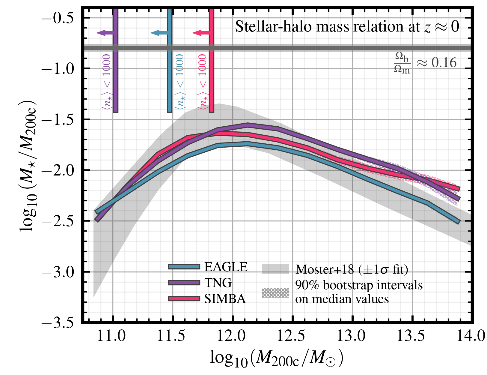
Figure 1: Median stellar to halo mass fractions as a function of $M_{\rm 200c}$ mass in EAGLE (blue), TNG (purple), and SIMBA (pink) at $z=0$. The inferred relation presented in Moster et al. (2018) $\pm 1\sigma$ from their fit is included for reference as a grey shaded region. In each of the simulations, the hatched shaded regions represent the $90\%$ confidence interval on the median from 100 bootstrap re-samplings in each bin. There is general agreement between the simulations and the Moster et al. (2018) relation, despite the simulations each utilising very different sub-grid physics.

3 The baryon budget between simulations

In this section, before presenting our analysis of gas flows between the simulations in §2.2, we compare static properties of the baryons within haloes in EAGLE, TNG, and SIMBA at $z=0$. Here, we compare our measurements the baryon content of haloes between simulations, and its breakdown between different components. We note that we reserve a detailed discussion of the link between these findings and previous studies for §5.1.

Fig. 1 shows the stellar mass relative to the halo mass as a function of halo mass, for central galaxies in each of the three simulations. For comparison, we show the relation derived by Moster et al. (2018), who use an empirical model that carefully connects observed galaxy properties to simulated dark matter haloes. In EAGLE, TNG and SIMBA, the stellar-halo mass ratios are calculated directly from the simulations, including star particles within a $30\,{\rm kpc}$ spherical aperture of the halo centre of potential, and normalising by the halo mass within the $R_{\rm 200c}$ radius, $M_{\rm 200c}$. We convert the virial masses used as the x-values in Moster et al. (2018) from the Bryan & Norman (1998) overdensity criterion to the $M_{\rm 200c}$ definition we use here with hmfcalc (Murray et al., 2013), however note that we do not adjust the Moster et al. (2018) $f_{\star}$ values at a given halo mass. We also note that the observations that constrain the Moster et al. (2018) empirical model are diverse, and subject to systematic uncertainties and projection effects which we do not attempt to mimic with our simulation-based measurements. Despite these differences in methodology, Fig. 1 illustrates that each simulation reproduces the reduced galaxy formation efficiency at low- and high- masses required to match observationally derived stellar mass functions (see also Somerville & Davé 2015; Davé et al. 2020). As noted above, and discussed in (Somerville & Davé, 2015), the relatively good agreement of the different simulations in spite of the very different implementation of sub-grid physics is largely due to the fact that a high weight is placed on reproducing these observational constraints when calibrating the sub-grid parameters.

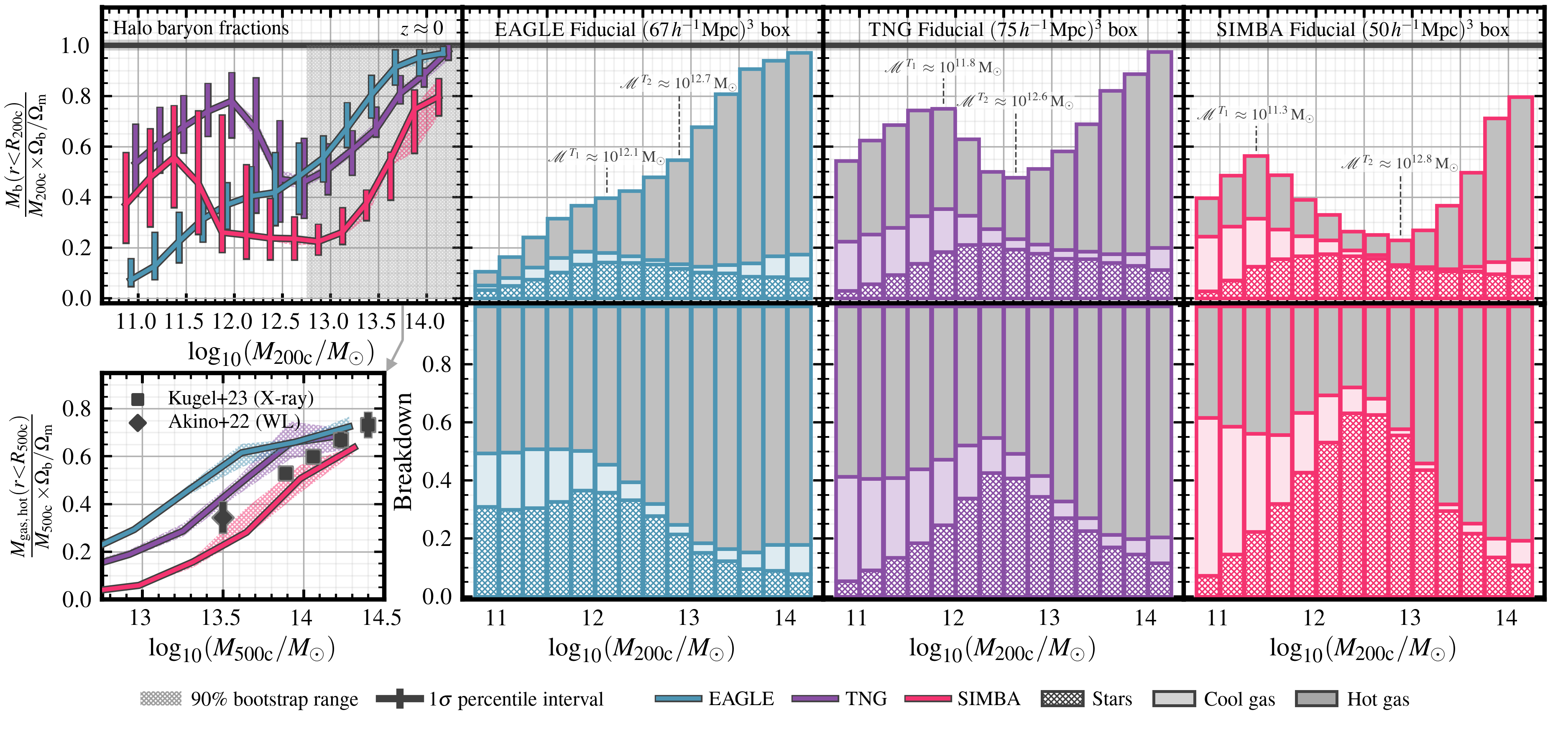
Figure 2: The baryon content of haloes at $z\approx 0$ in EAGLE (blue), TNG (purple) and SIMBA (pink). Top panel, $1^{\rm st}$ column: The median total baryon fraction within $R_{\rm 200c}$ (stars, gas, black holes) of haloes as a function of $M_{\rm 200c}$ mass. Bottom panel, $1^{\rm st}$ column: The gas fraction of haloes within $R_{\rm 500c}$ as a function of $M_{\rm 500c}$, shown in comparison to weak lensing observations from Akino et al. (2022) (diamond point); and X-ray data compiled in Kugel et al. (2023) (square points). Top panels, $2^{\rm nd}-4^{\rm th}$ columns: Total baryon content for each simulation within $R_{\rm 200c}$ broken down into stars (hatched bars), “cool” gas (coloured shaded bars), and “hot gas” (grey bars) in each simulation. In the top panels, this baryon content is normalised by $f_{\rm b}\times M_{\rm 200c}$. Bottom panels, $2^{\rm nd}-4^{\rm th}$ columns: These panels shows the same breakdown, but re-normalised by the actual baryonic mass in each halo, $M_{\rm bar}(r<R_{\rm 200c})$. In each of the simulations in the left-hand panel, error-bars represent the $16^{\rm th}-84^{\rm th}$ percentiles in halo baryon fractions for a given mass bin; the hatched regions represent the $90\%$ confidence interval on the median from 100 bootstrap re-samplings in each bin. While the simulations produce similar results for the stellar content of haloes at $z\approx 0$, the same cannot be said for the gaseous phase.

In Fig. 2, we compare the total baryon content of haloes at $z=0$ as a function of halo mass (top left hand panel), and in the remaining columns show how this baryon content is distributed between stars, cool gas, and hot gas in each of the simulations (as a fraction of total halo mass in the top panels, and as a breakdown of the total baryon content in the bottom panels). In each simulation, we define “cool gas” as the gas that is either considered star-forming, or below $5\times 10^{4}{\rm K}$, and “hot gas” as the remaining gas within $R_{\rm 200c}$ that does not meet this criteria. We do not illustrate the contribution from black holes in the breakdown panels as this component is typically very small. In the case of haloes with several galaxies within $R_{\rm 200c}$, we include the contribution from satellite galaxies in calculating the total baryonic mass in each reservoir. Also, unlike Fig. 1, in this plot the stellar content of the halo is determined using all stellar particles within $R_{\rm 200c}$, as opposed to the central $30{\rm kpc}$. This means in Fig. 2, the stellar component also includes contributions from intra-halo stars and satellite galaxies within $R_{\rm 200c}$. In each of the simulations, “cool gas” is defined to include gas within $R_{\rm 200c}$ that is either considered star-forming, or below a temperature cut of $5\times 10^{4}{\rm K}$. “Hot gas” is then defined to be all gas within $R_{\rm 200c}$ that does not meet the “cool gas” criteria, in effect constituting the CGM. The “cool gas” component is not decomposed further or post-processed to provide ${\rm H}$i and ${\rm H}_{2}$ content – for a dierct comparison of galaxy neutral hydrogen abundances in each of the simulations, we refer the reader to Davé et al. (2020). Furthermore, a phase decomposition of CGM gas as a function of halo mass is also presented for SIMBA in Sorini et al. (2022).

One of the striking differences between the simulations in terms of halo baryon fraction is their behaviour in the range $\log_{10}(M_{\rm 200c}/{\rm M}_{\odot})$ $\in[11.5,12.5]$. SIMBA and TNG roughly exhibit the same functional form in this mass range – halo baryon fractions increase with halo mass up to a turnover mass which we denote as ${\mathcal{M}}^{{\rm T}_{1}}$. Above ${\mathcal{M}}^{{\rm T}_{1}}$, halo baryon fractions decrease with halo mass until a second turnover mass, denoted by ${\mathcal{M}}^{{\rm T}_{2}}$, is reached. Above ${\mathcal{M}}^{{\rm T}_{2}}$, halo baryon fractions steadily rise again to the highest halo masses presented here at $\log_{10}(M_{\rm 200c}/{\rm M}_{\odot})$ $=$14. Physically, these transitions produce three distinct “regimes” in terms of the $M_{\rm 200c}-f_{\rm b}$ relation: (i) sub-${\mathcal{M}}^{{\rm T}_{1}}$, where baryon fractions increase with halo mass as a result of the decreasing efficiency of stellar feedback in removing gas from a deeper potential well; (ii) the transition range ${\mathcal{M}}^{{\rm T}_{1}}$ to ${\mathcal{M}}^{{\rm T}_{2}}$, where this trend reverses as AGN feedback grows in importance, and (iii) high mass $>$${\mathcal{M}}^{{\rm T}_{2}}$ haloes where similar to regime (i), the efficiency of AGN feedback in removing baryonic material decreases in very massive group-cluster mass haloes. We note that in the case of EAGLE, in the ${\mathcal{M}}^{{\rm T}_{1}}$-${\mathcal{M}}^{{\rm T}_{2}}$ range, there is only a slight flattening in halo baryon fractions with increasing mass, as opposed to a clear turnover. These halo baryon fractions, as well as the behaviour of simulation runs without AGN feedback (shown in Fig. 8 in Pillepich et al. 2018 for TNG, and Fig. 7 in Correa et al. 2018a for EAGLE) indicate that AGN activity is responsible for this turnover/flattening behaviour respectively between ${\mathcal{M}}^{{\rm T}_{1}}$-${\mathcal{M}}^{{\rm T}_{2}}$.

At halo masses below $\log_{10}(M_{\rm 200c}/{\rm M}_{\odot})$ $\approx 11.5$, corresponding to sub-${\mathcal{M}}^{{\rm T}_{1}}$ masses, the left hand panel of Fig. 2 demonstrates that all of the simulations presented have total baryon fractions that increase with halo mass. While this behaviour with halo mass is the same, the baryon fractions themselves are markedly different. In this mass regime, the fiducial L100-REF EAGLE model predicts the lowest baryon fractions of all the simulations presented. At a halo mass of $\log_{10}(M_{\rm 200c}/{\rm M}_{\odot})$ $\approx$11, the L100-REF model predicts a median halo baryon fraction of $\approx 15\%$ of the universal baryon fraction ($\Omega_{\rm b}/\Omega_{\rm m}\approx 0.16$). While we do not display the results here, we note that in the L25-RECAL model at this mass, halo baryon fractions are slightly higher at $\approx 30\%$, though still lower than the corresponding baryon fraction predictions from SIMBA at $\approx 40\%$ of the expected cosmological baryon fraction. TNG predicts the highest halo baryon fractions at this mass, at $\approx 60\%$ of the universal value (see also Davies et al. 2019a, b).

In this sub-${\mathcal{M}}^{{\rm T}_{1}}$ mass regime, we also note significant differences in the way that this baryonic matter is partitioned between the simulations. In the fiducial EAGLE model, the low overall baryon fractions mean that in order to match the expected stellar content of haloes, stars make up over $25\%$ of the baryonic content, compared to SIMBA and TNG where the stellar component only represents $\lesssim 10\%$ of the baryonic matter. For halo masses below $\log_{10}(M_{\rm 200c}/{\rm M}_{\odot})$ $\approx 11.5$, we note that the EAGLE L100-REF run predicts very low halo cool gas content – always less than half of the predicted stellar content. This is not the case in TNG and SIMBA, where the stellar to cool gas mass ratio is near unity in this mass range. Davé et al. (2020) show that the EAGLE fiducial run underpredicts the observed $z=0$ ${\rm H}$iMF from ALFALFA observations by $\approx 0.5\,{\rm dex}$ (Jones et al., 2018); but matches the local CO luminosity function from Saintonge et al. (2017) fairly well (see also Lagos et al. 2015). This suggests that the fiducial EAGLE run lacks the gas associated with the more diffuse atomic phase at $z=0$, however this result is heavily dependent on how gas phases are partitioned in post-processing. While not directly shown in this Figure, we remark that the L25-RECAL EAGLE model produces a better match to the local ${\rm H}$iMF; and that for $z\geq 1$, that the EAGLE L100-REF and L25-RECAL models are consistent with regard to predicted ${\rm H}$i and ${\rm H}_{2}$ mass functions.

While SIMBA and TNG predict a similar functional form for baryon fractions across halo mass, their normalisation and the location of transition masses ${\mathcal{M}}^{{\rm T}_{1}}$ and ${\mathcal{M}}^{{\rm T}_{2}}$ are markedly different (as also found in Ni et al. 2023; Delgado et al. 2023; Crain & van de Voort 2023). In TNG, the first transition mass occurs at $\log_{10}($${\mathcal{M}}^{{\rm T}_{1}}$$/{\rm M}_{\odot})\approx 11.8$; while in SIMBA, the transition occurs at much lower halo mass, $\log_{10}($${\mathcal{M}}^{{\rm T}_{1}}$$/{\rm M}_{\odot})\approx 11.3$. Furthermore, in TNG the second transition mass occurs at $\log_{10}($${\mathcal{M}}^{{\rm T}_{2}}$$/{\rm M}_{\odot})=12.6$; while in SIMBA, halo baryon fractions do not increase until $\log_{10}($${\mathcal{M}}^{{\rm T}_{2}}$$/{\rm M}_{\odot})\approx 12.8$. In this transition range, halo baryon fractions in TNG are, on average, 20%-50% higher than those measured in SIMBA. Furthermore, at $\log_{10}(M_{\rm 200c}/{\rm M}_{\odot})$ $=$14, baryon fractions in SIMBA only reach $\approx$70% of $\Omega_{\rm b}/\Omega_{\rm m}$, while haloes in TNG haloes approach this universal value very closely. Instead of a turnover, EAGLE predicts a flattening in halo baryon fractions between $\log_{10}($${\mathcal{M}}^{{\rm T}_{1}}$$/{\rm M}_{\odot})\approx 12.1$ and $\log_{10}($${\mathcal{M}}^{{\rm T}_{2}}$$/{\rm M}_{\odot})\approx 12.7$. In this transition range, the drop in TNG baryon fractions meets the slowly rising EAGLE baryon fractions at the ${\mathcal{M}}^{{\rm T}_{2}}$ transition point. Above ${\mathcal{M}}^{{\rm T}_{2}}$, EAGLE and TNG agree very well in terms of predicted baryon fractions as a function of halo mass.

In the high-mass regime, it is possible to compare predictions for halo gas content with observations. In Kugel et al. (2023), a number of carefully compiled X-ray and weak lensing (WL) observations were used to calibrate a large-volume cosmological simulation, FLAMINGO. Such observational datasets are nominally cast as (hot) gas fractions within $R_{\rm 500c}$, as a function of $M_{\rm 500c}$, representing a slightly shrunken aperture relative to the rest of our measurements. In the bottom left panel of Figure 2, we present like-for-like measurements of hot halo gas content in each of the simulations within $R_{\rm 500c}$, and compare with this set of observations compiled in Kugel et al. (2023). We refer the reader to this study for a detailed explanation of the curated dataset, noting that we only make use of the WL data from Akino et al. (2022), and that the relevant X-ray datasets come from the following studies: Vikhlinin et al. (2006); Maughan et al. (2008); Rasmussen & Ponman (2009); Sun et al. (2009); Pratt et al. (2010); Lin et al. (2012); Laganá et al. (2013); Sanderson et al. (2013); Gonzalez et al. (2013); Lovisari et al. (2015); Pearson et al. (2017); Lovisari et al. (2020). As above, we define “hot” gas as any gas elements with a temperature $T\geq 5\times 10^{4}$. We note that this choice of threshold does not significantly influence gas fractions in this mass range, as the majority of gas is at or above halo virial temperature (see top panels). Regardless, we stress that this selection is unlikely to exactly mimic the gas accounted for in the observations, however, does allow us to understand the difference between simulation predictions and their broad agreement with observations. Our measurements between $M_{\rm 500c}=10^{13.5}{\rm M}_{\odot}-M_{\rm 500c}=10^{14.5}{\rm M}_{\odot}$ indicate that median halo gas fractions in TNG and EAGLE are slightly higher than the compiled observations (more so in EAGLE), and slightly lower than observations in SIMBA. The range of predictions from the simulations is largest between $M_{\rm 500c}=10^{13}{\rm M}_{\odot}-M_{\rm 500c}=10^{14}{\rm M}_{\odot}$, while at higher masses ($M_{\rm 500c}\approx 10^{14.5}{\rm M}_{\odot}$), the gas fractions tend towards a tighter range. For reference, we note that the offset between $M_{\rm 200c}$ and $M_{\rm 500c}$ halo mass measurements is relatively constant at $\approx 0.15$ dex in this mass range. While the X-ray datasets extend to higher masses, there is a scarcity of cluster-mass haloes in the simulations to used for this study due to their box size.

In Appendix D, we show a breakdown of the baryon content of haloes at $z=2$, finding that the qualitative behaviour of the simulations in relation to baryon fraction across halo mass remains similar to the results presented here at $z=0$, with a universal shift to higher halo baryon fractions. The transition masses ${\mathcal{M}}^{{\rm T}_{1}}$ and ${\mathcal{M}}^{{\rm T}_{2}}$ remain similar in EAGLE and TNG at $z=2$ compared to $z\approx 0$ galaxies; though this is not the case for SIMBA. In SIMBA, the transition masses are higher than at $z=0$, with $\log_{10}($${\mathcal{M}}^{{\rm T}_{1}}$$/{\rm M}_{\odot})=12.2$ and $\log_{10}($${\mathcal{M}}^{{\rm T}_{2}}$$/{\rm M}_{\odot})=12.8$ at $z=2$ (see also Fig. 7 in Sorini et al. 2022).

To aid in the interpretations of the gas flow measurements in the following section (§4), in Appendices B and C we provide radial density and temperature profiles of central galaxies in each of the simulations. Together with the figures contained in this section, these radial profiles provide additional information about the spatial distribution and properties of gas within haloes in each of the simulations.

4 Gas flows through the ISM, CGM, and IGM

In this section, we aim to identify the physical mechanisms behind the differences in the baryon budget predicted by the EAGLE, TNG and SIMBA simulations as explored in §3. Our method for measuring gas flow rates is detailed in §2.2. We note that for the purposes of this analysis, we do not enforce any additional selection cuts to classify elements as inflow or outflow other than the sign of their radial velocity.

4.1 Ejective feedback: gas outflow rates as a function of scale

In Fig. 3, we display measurements of galaxy outflow rates at the ISM scale in a form commonly presented in previous literature: the ISM scale mass loading factor, $\eta=\dot{M}_{\rm out}/{\rm SFR}$, where $\langle\dot{M}_{\rm out}\rangle$ is the mean gas outflow rate, and $\langle\dot{M}_{\star}\rangle$ is the mean star formation rate. We begin by comparing the mass loading results between simulations at $z\approx 2$, which builds a picture for the operation of gas flows at the epoch of maximum star formation rate density (Madau & Dickinson, 2014). In the bottom panel of Fig. 3, we also compare the median specific star formation rate ($\dot{M}_{\star}/M_{\star}$) of galaxies. This assists in understanding the influence of star formation rate on the mass loading measurements provided in the top panel. In the bottom panel, we also include a hatched grey region which represents an indicative “quenched” region where the specific star formation rate drops below $\log_{10}({\rm sSFR}/{\rm yr^{-1}})={-11+0.5z}$ (Furlong et al., 2015).

We define the stellar mass of a galaxy in the same way as Fig. 1, including all star particles within $30{\rm\,kpc}$ of the halo centre of potential. Similarly, the star formation rates we use in calculating mass loading are evaluated with gas within $30{\rm kpc}$ of the galaxy centre, which is fixed regardless of the scale that we measure outflow rates. We define the “ISM” scale by measuring gas flows across a spherical boundary at $r=0.25\times R_{\rm 200c}$, which we consider to be the outer scale of the ISM. We stress that we do not enforce a minimum radial velocity for outflow gas; meaning that while we do select slow-moving outflow particles, these outflow values are fair to compare between the simulations and represent the true mass flux at each scale. Furthermore, for the mass flow rate measurements at the scale of the ISM, we do not require the gas to be “cool” to be included in the calculation. This choice is made to simplify subsequent comparisons with gas flows at larger scales, where in many cases the majority of the gas has been heated to near the virial temperature of the halo (see Appendix C).

We follow the approach of Mitchell et al. (2020) (based on arguments presented in Neistein et al. 2012) in calculating mass loading: instead of comparing $\eta\equiv\dot{M}_{\rm out}/{\rm SFR}$ for each halo individually, we calculate $\eta$ for each halo mass as the mean outflow rate in each halo mass bin divided by the mean star formation rate in the bin. Neistein et al. (2012) demonstrate that this method correctly predicts the average rate of mass exchange when integrated over time, and also mitigates the impact of discreteness noise that would otherwise influence the results. We note that the percentile ranges displayed in the top panel of Fig. 3 correspond to the range of mass loading values predicted based on the $16^{\rm th}$ and $84^{\rm th}$ percentiles of mass outflow rate in a given stellar mass bin, without including variance in star formation rates at a given mass.

For reference, in Fig. 3, we also include indicative $\eta$ scalings with $V_{\rm c}\equiv\sqrt{GM_{\rm 200c}/R_{\rm 200c}}$ (halo circular velocity): a “momentum conserving” scenario with $\eta\propto V_{\rm c}^{-1}\propto M_{\rm 200c}^{-1/3}$; and an “energy conserving” scenario with $\eta\propto V_{\rm c}^{-2}\propto M_{\rm 200c}^{-2/3}$ as dashed and dash-dotted lines respectively (see Murray et al. 2005 for derivation).

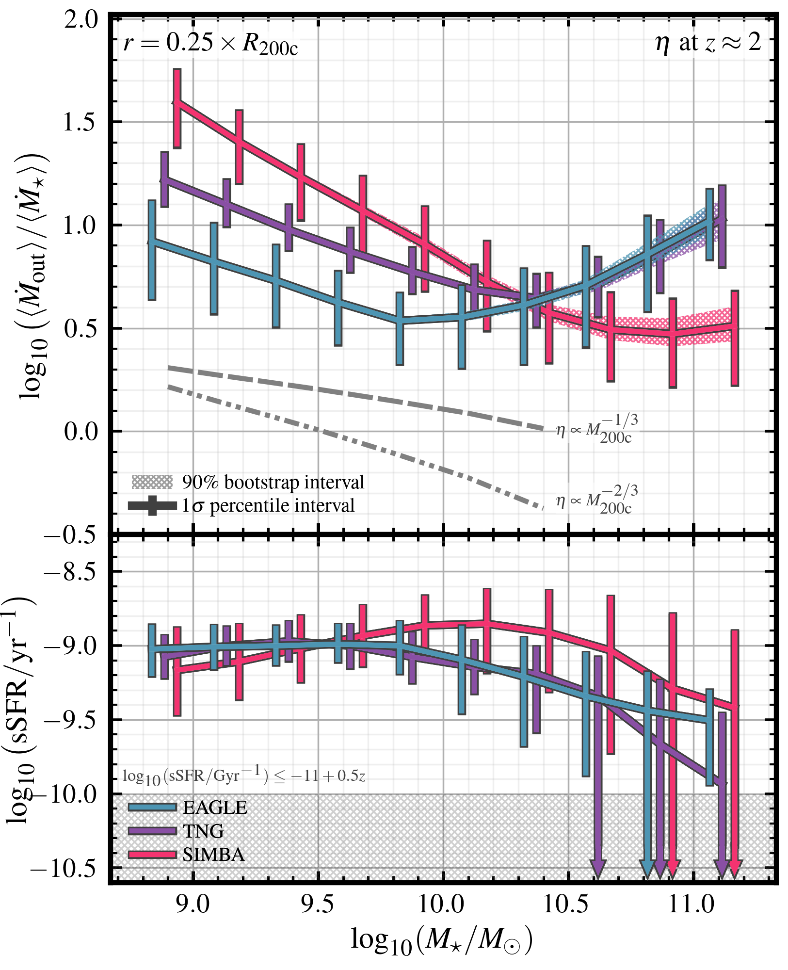
Figure 3: Mass loading ($\eta$) and specific star formation rates (${\rm sSFR}$) at $z\approx 2$ as a function of stellar mass in EAGLE (blue), TNG (purple) and SIMBA (pink). Top panel: averaged ISM-scale ($r=0.25R_{\rm 200c}$) mass loading (see text for definition) as a function of stellar mass. Bottom panel: mean specific star formation rate as a function of stellar mass in each of the simulations. In the top panel, the error-bars displayed correspond to the range of measured mass loading values based on the $16^{\rm th}$ and $84^{\rm th}$ percentiles of mass outflow rate in a given stellar mass bin. In the bottom panel, the error-bars correspond to the $16^{\rm th}-84^{\rm th}$ percentile range of ${\rm sSFR}$ at a given mass. In both panels, coloured hatched regions correspond to the bootstrap-generated $90\%$ confidence interval on the respective averages at a given mass. $\eta$ scales negatively with $M_{\star}$ for all simulations below $M_{\star}\approx 10^{10}{\rm M}_{\odot}$, however the $\eta$ values in this mass range can vary between simulations by $\gtrsim 0.5\,$dex on average.

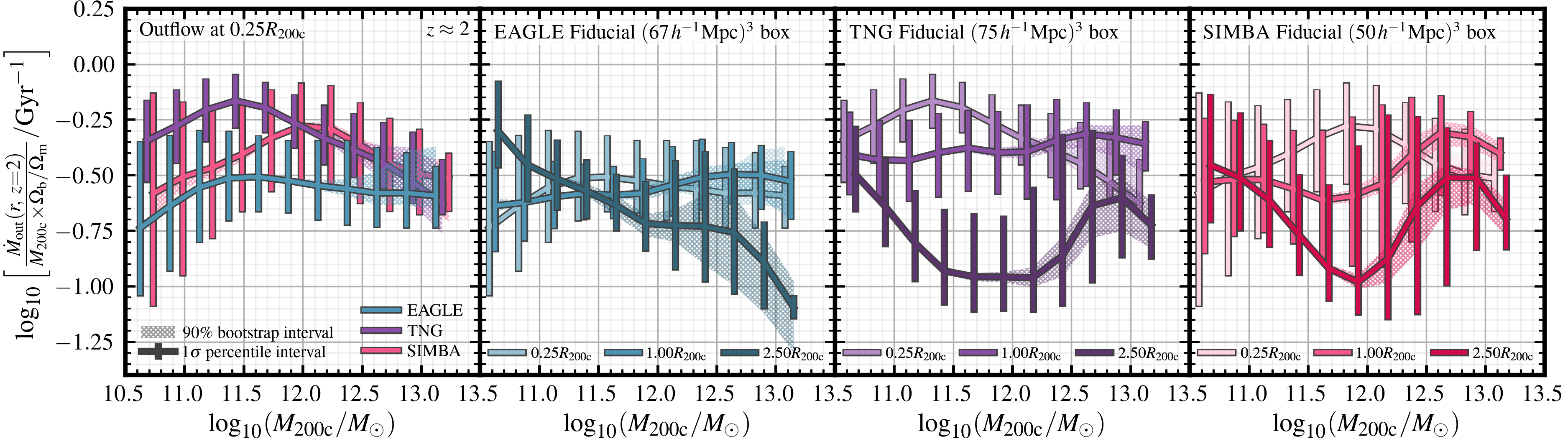
Figure 4: Mass outflow rates as a function of $M_{\rm 200c}$ at $z\approx 2$ in EAGLE (blue), TNG (purple) and SIMBA (pink). Mass outflow rates are normalised by $f_{\rm b}\times M_{\rm 200c}$ in each case to indicate gas outflow “efficiency” across different mass scales. Left panel: Outflow efficiency at the ISM scale, compared between the simulations. Panels 2-4: Outflow efficiencies at different scales in EAGLE, TNG, and SIMBA respectively. In each of these panels, ISM-scale outflows are plotted with lighter colours, halo-scale outflowsare plotted in medium colours, and larger-scale outflows are plotted in darker colours. In all panels, error-bars correspond to the $16^{\rm th}-84^{\rm th}$ percentile range in outflow rates at a given mass, and hatched regions correspond to the bootstrap-generated $90\%$ confidence interval on the medians at a given mass. SF-driven outflows reach the greatest scale in EAGLE, while AGN-driven outflows reach the greatest scale in SIMBA.

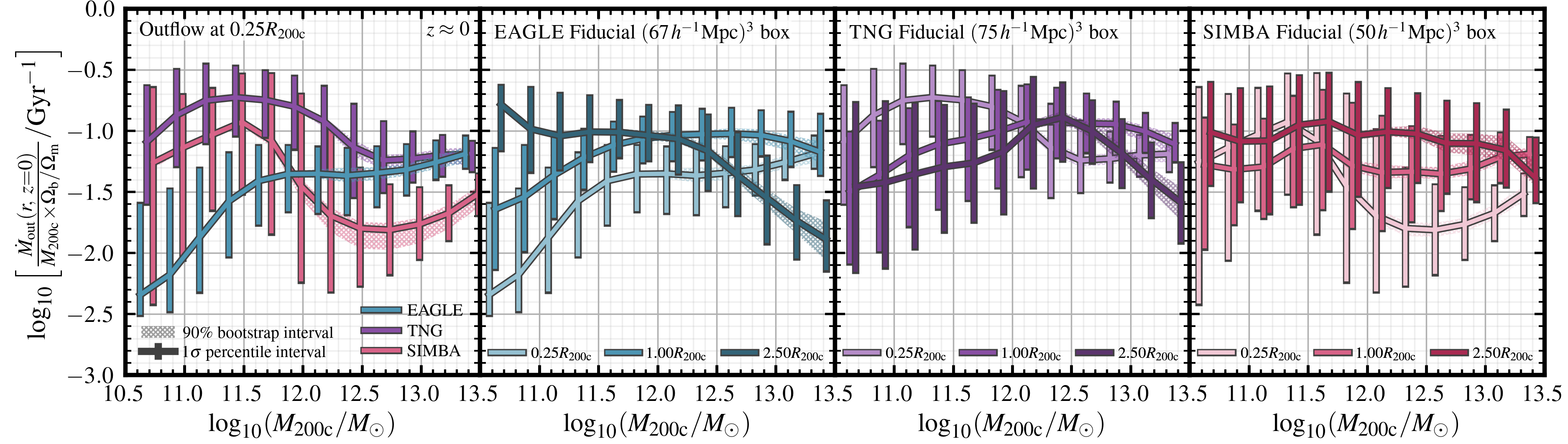
Figure 5: Mass outflow rates as a function of $M_{\rm 200c}$ at $z\approx 0$ in EAGLE (blue), TNG (purple) and SIMBA (pink). Mass outflow rates are normalised by $f_{\rm b}\times M_{\rm 200c}$ in each case to indicate gas outflow “efficiency” across different mass scales. Left panel: Outflow efficiency at the ISM scale, compared between the simulations. Panels 2-4: Outflow efficiencies at different scales in EAGLE, TNG, and SIMBA respectively. In each of these panels, ISM-scale outflows are plotted with lighter colours, halo-scale outflowsare plotted in medium colours, and larger-scale outflows are plotted in darker colours. In all panels, error-bars correspond to the $16^{\rm th}-84^{\rm th}$ percentile range in outflow rates at a given mass, and hatched regions correspond to the bootstrap-generated $90\%$ confidence interval on the medians at a given mass. EAGLE predicts efficient SF-driven ejection of gas from haloes, while TNG and SIMBA predict an intra-halo “recycling” scenario for SF-affected gas. AGN-driven outflows reach the greatest scale in SIMBA.

At the ISM-scale of $r=0.25R_{\rm 200c}$ in the top panel of Fig. 3, it is clear that each of the simulations predicts a similar negative scaling in $\eta=\dot{M}_{\rm out}/{\rm SFR}$ as a function of $M_{\star}$, until a turnover mass where outflows begin to pick up relative to star formation rates (also demonstrated in Nelson et al. 2019 and Mitchell et al. 2020 for TNG and EAGLE respectively, though using different scales and methodologies). The turnover mass differs slightly between simulations – in EAGLE and TNG, the turnover occurs at $M_{\star}\approx 10^{10}{\rm M}_{\odot}$ and $M_{\star}\approx 10^{10.3}{\rm M}_{\odot}$ respectively; with $\eta$ values at the turnover masses reaching a minimum of $\eta\approx 10^{0.5}$ and $\eta\approx 10^{0.7}$ respectively. In SIMBA, the turnover is more gradual, with the minimum average mass loading occurring closer to $M_{\star}\approx 10^{11}{\rm M}_{\odot}$. Folding in the stellar-halo mass relation in each of the simulations, in EAGLE and TNG the turnover mass occurs at $\log_{10}(M_{\rm 200c}/{\rm M}_{\odot})$ $\approx 11.8-12$, while in SIMBA, the turnover occurs at a slightly higher mass of $\log_{10}(M_{\rm 200c}/{\rm M}_{\odot})$ $\approx 12.4$ at $z\approx 2$ (as is also the case for halo baryon content).

Below the turnover mass, the scaling of $\eta$ with mass for each of the simulations falls between the expected “momentum conserving” ($\eta\propto M_{\rm 200c}^{-1/3}$) and “energy conserving” ($\eta\propto M_{\rm 200c}^{-2/3}$) scaling relations. The relation is steepest in SIMBA, for which $\eta$ approximately follows $M_{\rm 200c}^{-2/3}$, and is closer to $M_{\rm 200c}^{-1/2}$ in EAGLE and TNG. The mass outflow rate from the ISM per unit star formation rate in this mass range is highest in SIMBA, which predicts $\eta=10^{1.6}$ at $M_{\star}\approx 10^{9}{\rm M}_{\odot}$, followed by TNG predicting approximately one third of this outflow rate at $\eta=10^{1.2}$, and EAGLE predicting approximately half of the TNG outflow rates at $\eta=10^{0.9}$, for the same stellar mass.

The higher mass loading factors predicted in TNG and SIMBA at this scale are likely a result of the combination of input mass loading prescriptions, velocities, and the temporarily decoupled nature of these wind gas elements. Even though the wind gas elements in both simulations are likely to have recoupled before reaching the scale where we measure outflow rates ($0.25\times R_{\rm 200c}$), the ability of these gas elements to escape the densest regions of the ISM without losing as much momentum means that the mass flux at this scale can remain quite high. Nelson et al. (2019) show in relation to the TNG50 simulation that while the velocity and $\eta$ of SF-driven feedback are prescribed at injection, the way in which these outflows propagate to larger scales is non-trivial. The mass loading factors presented at the ISM scale agree with the measurements at $10\,{\rm kpc}$ presented in Nelson et al. (2019), and the SIMBA mass loading at this scale agrees with the input mass loading prescription from Anglés-Alcázar et al. (2017b) taken from the FIRE simulations. In comparison, in EAGLE, thermal SF-driven outflows do not have prescribed velocities or mass loading. The feedback energy is deposited purely thermally, and the large temperature boosts ($\Delta T_{\rm SF}=10^{7.5}\,{\rm K}$) and associated pressure produce strong outflows.

Above the mass turnover where AGN feedback becomes the dominant ejection mechanism, there are further clear differences between mass loading in the simulations. TNG demonstrates the steepest upturn in ISM-scale mass loading with halo mass, reaching $\eta=10^{1.7}$ at $\log_{10}(M_{\rm 200c}/{\rm M}_{\odot})$ $=13$. At this same mass, EAGLE predicts a mass loading of approximately half the TNG value at $10^{1.4}$, and SIMBA predicts mass loading at one tenth of the EAGLE value at $10^{0.6}$ (corresponding to the increased transition mass at which AGN feedback becomes efficient as per Fig. 2). The lower $\eta$ values at high mass in SIMBA are likely linked to the onset of jet-mode feedback, which injects more energy than the QSO-mode feedback with the same momentum flux, corresponding to a much lower mass loading factor relative to the BH accretion rate.

Comparing the median specific star formation rates in the bottom panel of Fig. 3, we note that there is broad agreement between the simulations in terms of the shape of the star formation main sequence. There are, however, small quantitative differences between the simulations – for instance, the median specific star formation rate in SIMBA at $M_{\star}\approx 10^{9}{\rm M}_{\odot}$ sits $0.1-0.2$ dex below EAGLE and TNG, and sits $0.3-0.4$ dex above EAGLE and TNG for $M_{\star}\approx 10^{10.2}-10^{10.7}{\rm M}_{\odot}$. Together, these slight differences in star formation activity complicate comparisons between outflow behaviour in the simulations using $\eta$. Furthermore, instantaneous measurements of mass loading do not account for the delay between star formation and the associated feedback. As such, for the remainder of this paper, we quote flow rates without normalizing by star formation rate. Additionally, citing the (slight) differences in the stellar-halo mass relation between simulations as presented in Fig. 1, we choose to compare the baryon cycle between simulations as a function of halo mass rather than stellar mass for the remainder of this work. Given the very similar underlying cosmological parameters, the form of the halo mass functions in the simulations are very closely matched; meaning that using halo mass as the dependent variable allows us to fairly compare the simulations at a set depth of gravitational potential well.

In Fig. 4 and 5, we show the raw outflow rates for central galaxies in each simulation as a function of halo mass, normalised by $\Omega_{\rm b}/\Omega_{\rm m}\times M_{\rm 200c}$ at $z=2$ and $z=0$ respectively (“outflow efficiency”). In the left hand panels, we show these outflow rates at the ISM scale ($0.25\times R_{\rm 200c}$). In the remaining panels for each simulation, we show outflow rates at the ISM scale, the halo scale (defined at $1.00\times R_{\rm 200c}$), and at the IGM scale (defined at $2.50\times R_{\rm 200c}$).

The values of outflow efficiency indicate the inverse of the time-scale that would be required for a gas mass of $M_{\rm 200c}\times\ \Omega_{\rm b}/\Omega_{\rm m}$ to be removed at this scale. In the left-hand panels of Fig. 4 and 5, we compare median outflow rates in each of the simulations at the ISM scale ($0.25\times R_{\rm 200c}$). In each of the remaining panels, for each of the simulations we compare outflow rates at three scales: $r=0.25\times R_{\rm 200c}$, $r=1.00\times R_{\rm 200c}$, and $r=2.50\times R_{\rm 200c}$. Firstly, focusing on the left-hand panels which compare the simulations at the ISM scale, we note that at both redshifts, below $\log_{10}(M_{\rm 200c}/{\rm M}_{\odot})$ $\approx 12$, total outflow rates in TNG are actually higher than in SIMBA, in contrast to the mass loading factors which are higher in SIMBA. This can be explained by the slightly lower normalisation of the $M_{\star}-{\rm sSFR}$ relation in SIMBA compared to TNG (see Fig. 3 for sSFR measurements at $z\approx 2$ and Davé et al. 2019 for measurements at $z\approx 0$) – meaning that galaxies in SIMBA eject more gas per unit SFR compared to TNG galaxies, but have lower absolute total outflow rates. This highlights the fact that if a galaxy is gas poor, the amount of gas available for removal is proportionally reduced.

It is when we analyse the behaviour of outflow rates as a function of scale as per the right-hand panels in Fig. 4 and 5, that dramatic differences between gas flows in the simulations begin to emerge. We first focus on the $z\approx 2$ case, as presented in Fig. 4. Below $\log_{10}(M_{\rm 200c}/{\rm M}_{\odot})$ $\approx 11$ in EAGLE (where stellar feedback is dominant in driving outflows), mass outflow rates at the ISM ($0.25\times R_{\rm 200c}$), halo ($1\times R_{\rm 200c}$), and IGM ($2.5\times R_{\rm 200c}$) scales remain very similar. This indicates that the galactic winds in EAGLE can travel to at least $2.5\times R_{\rm 200c}$ at $z\approx 2$ before stalling and falling back.

Unlike the picture in EAGLE, below $\log_{10}(M_{\rm 200c}/{\rm M}_{\odot})$ $\approx 12$ outflow rates decrease with increasing scale in TNG. At $\log_{10}(M_{\rm 200c}/{\rm M}_{\odot})$ $\approx 11.5-12$ in TNG, outflow rates at $r=2.5\times R_{\rm 200c}$ are just $10\%$ of those measured at $r=0.25\times R_{\rm 200c}$. We do note, however, that this stalling is less obvious in lower-mass systems with $\log_{10}(M_{\rm 200c}/{\rm M}_{\odot})$ $\approx 11$ – at this mass, average outflow rates at $R_{\rm 200c}$ are $\approx 50\%$ of that measured at the ISM-scale. In general, the stalling of SF-driven outflows in TNG is related to the velocities imparted to wind particles at injection, which scale with $\sigma_{\rm DM}$, which is almost always below the escape velocity of the halo (Nelson et al., 2019). This means that SF-driven outflows in TNG are ultimately confined to recycle within the halo, except for perhaps in the context of very low-mass haloes ($\lesssim 10^{10.5}\,{\rm M}_{\odot}$). In SIMBA, the picture for SF-driven outflows is somewhere between EAGLE and TNG. At low halo masses ($M_{\rm 200c}\approx 10^{10.5}\,{\rm M}_{\odot}$) outflows are able to reach a similar scale as predicted in EAGLE ($2-3\times R_{\rm 200c}$), while towards larger masses ($M_{\rm 200c}\approx 10^{12}\,{\rm M}_{\odot}$) outflows largely stall before reaching $R_{\rm 200c}$. This result is again a direct consequence of the assumed wind velocities at injection, which in SIMBA are taken from Muratov et al. (2015).

Above $\log_{10}(M_{\rm 200c}/{\rm M}_{\odot})$ $\approx 12.5$ at $z\approx 2$, where AGN feedback begins to dominate the driving of outflows, the behaviour between the simulations is also different. In EAGLE, the outflow rate at the ISM and halo scales remain similar in this mass range, but drop dramatically at the $2.5\times R_{\rm 200c}$ scale, with $\dot{M}_{\rm out}$ at $2.5\times R_{\rm 200c}$ approximately one tenth of the value at $R_{\rm 200c}$ in halos with mass $\log_{10}(M_{\rm 200c}/{\rm M}_{\odot})$ $\approx 13$. This indicates that AGN-driven outflows in EAGLE tend to stall near or just outside the virial radius at $z\approx 2$, and seldom reach larger scales. TNG shows qualitatively similar behaviour, but a less dramatic drop off in outflow rate with increasing scale. SIMBA actually shows a monotonically increasing outflow rate with increasing scale at $\log_{10}(M_{\rm 200c}/{\rm M}_{\odot})$ $\approx 11.5-13$, and a constant outflow rate from $R_{\rm 200c}$ to $2.5\times R_{\rm 200c}$ at higher halo masses.

This indicates that the outflows driven by AGN in TNG and SIMBA are more powerful in terms of spatial reach, likely related to the fact that in both of these models, AGN feedback is implemented with a significant kinetic component rather than just thermally as in the case of EAGLE.

Moving to the $z\approx 0$ Universe in Fig. 5, we note that the qualitative differences between simulations remain similar to the $z\approx 2$ picture at the ISM scale, however the disparities between how the outflows propagate across scales become even more pronounced. In the left-hand panel, we can see that the normalisation of gas flow rates relative to halo mass are much lower than at $z\approx 2$, with longer dynamical time-scales and lower gas densities at this epoch. One exception to this is the strength of AGN-driven outflows in SIMBA – which are much stronger at $z\approx 0$, and also become efficient at lower halo masses. This is likely a result of jet-mode feedback switching on more frequently at low redshift due to the requirement of low Eddington ratios (typical Eddington ratios decline at low redshift; see Thomas et al. 2019, Fig. 5).

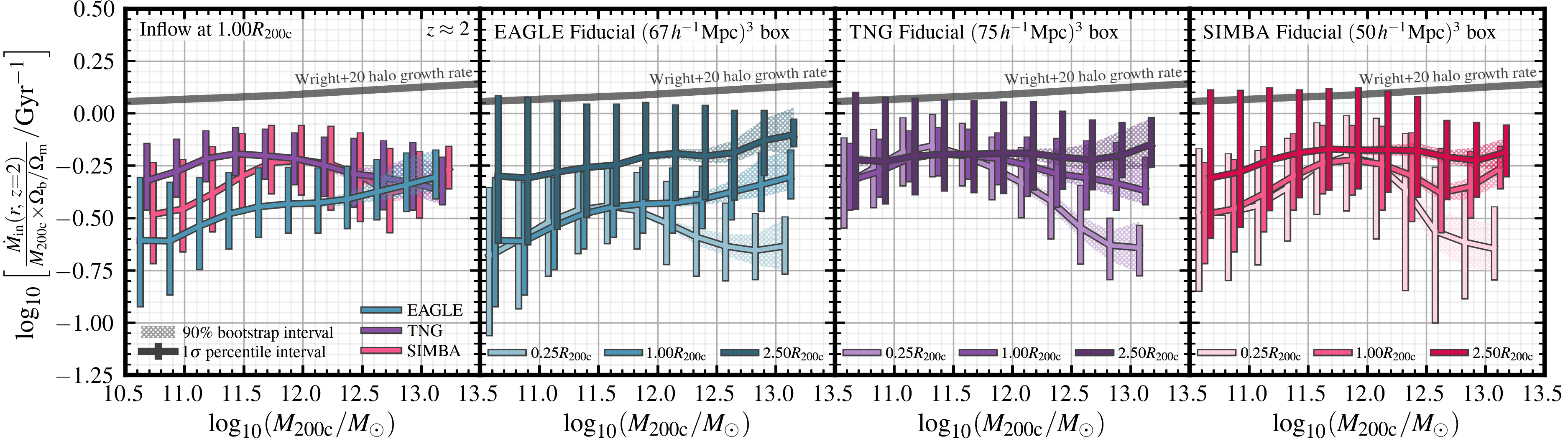
Figure 6: Mass inflow rates as a function of $M_{\rm 200c}$ at $z\approx 2$ in EAGLE (blue), TNG (purple) and SIMBA (pink). Inflow rates are normalised by $f_{\rm b}\times M_{\rm 200c}$ in each case to represent gas inflow “efficiency” across different mass scales. Left panel: Inflow efficiency at the halo scale, compared between the simulations. Panels 2-4: Inflow efficiencies at different scales in EAGLE, TNG, and SIMBA respectively. In each of these panels, ISM-scale inflows are plotted with lighter colours, halo-scale inflows are plotted in medium colours, and IGM-scale inflows are plotted in darker colours. We also include measurements from Wright et al. (2020) indicating the gas accretion rate expected if gas inflows perfectly traced the infall of DM in grey. In all panels, error-bars correspond to the $16^{\rm th}-84^{\rm th}$ percentile range in inflow rates at a given mass, and hatched regions correspond to the bootstrap-generated $90\%$ confidence interval on the medians at a given mass. All simulations predict that AGN feedback has a strong preventative impact on gas accretion at the ISM scale, however there is considerable variability between the preventative impact of stellar feedback.

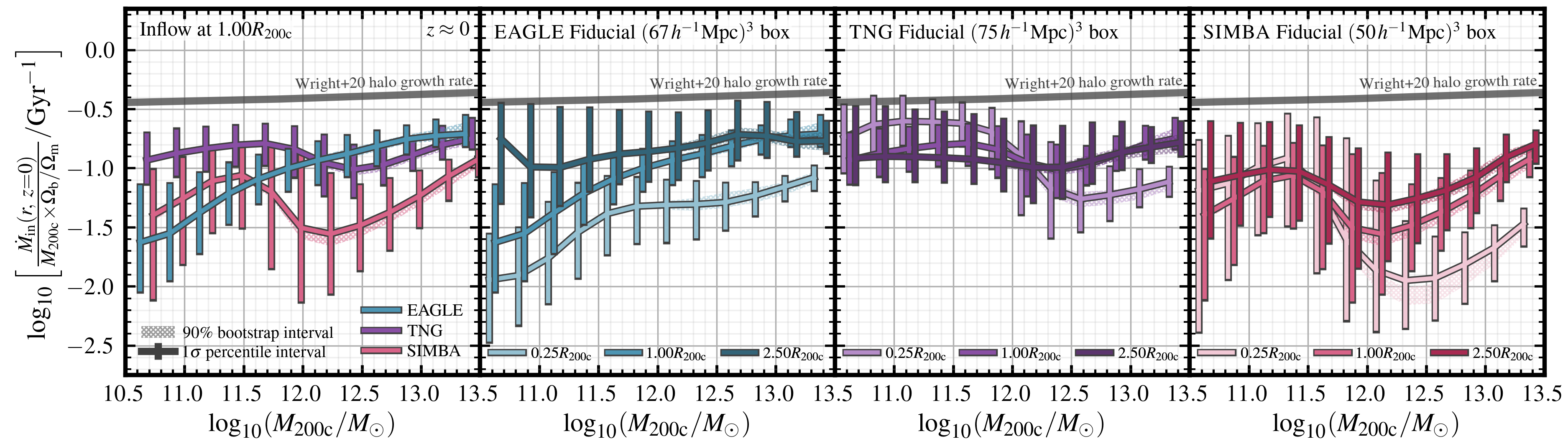
Figure 7: Mass inflow rates as a function of $M_{\rm 200c}$ at $z\approx 0$ in EAGLE (blue), TNG (purple) and SIMBA (pink). Inflow rates are normalised by $f_{\rm b}\times M_{\rm 200c}$ in each case to represent gas inflow “efficiency” across different mass scales. Left panel: Inflow efficiency at the halo scale, compared between the simulations. Panels 2-4: Inflow efficiencies at different scales in EAGLE, TNG, and SIMBA respectively. In each of these panels, ISM-scale inflows are plotted with lighter colours, halo-scale inflows are plotted in medium colours, and IGM-scale inflows are plotted in darker colours. We also include measurements from Wright et al. (2020) indicating the gas accretion rate expected if gas inflows perfectly traced the infall of DM in grey. In all panels, error-bars correspond to the $16^{\rm th}-84^{\rm th}$ percentile range in inflow rates at a given mass, and hatched regions correspond to the bootstrap-generated $90\%$ confidence interval on the medians at a given mass. The prevention of gas inflow at the halo-scale due to stellar feedback is strongest in EAGLE, followed by SIMBA, then TNG. The prevention of gas inflow at the halo-scale due to AGN feedback is strongest in SIMBA, followed by TNG, then EAGLE.

One very interesting feature at $z\approx 0$ in the EAGLE simulations is the apparent entrainment of outflowing gas with increasing scale. We find that at $\log_{10}(M_{\rm 200c}/{\rm M}_{\odot})$ $\approx 11$, the mass outflow rate at $2.5\times R_{\rm 200c}$ is over 10 times higher than that at $0.25\times R_{\rm 200c}$ in EAGLE at $z\approx 0$. This means that the stellar feedback driven outflows in EAGLE are not only able to reach scales beyond the halo, but also entrain mass along the way. Mitchell et al. (2020) have previously investigated this effect, finding that the out-flowing gas is significantly over-pressurised relative to the ambient CGM at $z=0$. This causes the tenuous material in the CGM to be swept up with the bulk flow.

As demonstrated in Fig. 4, in the regime dominated by stellar feedback, $M_{\rm halo}\lesssim 10^{12}{\rm M}_{\odot}$, we find that in EAGLE there is minimal mass entrainment in outflows at $z\approx 2$ compared to $z\approx 0$ (with the exception of haloes below $10^{11}{\rm M}_{\odot}$, where outflows at $2.5\times R_{\rm 200c}$ are enhanced relative to the ISM and halo scale by a factor of a few). This means that while the outflows do not significantly stall for halo masses of $\log_{10}(M_{\rm 200c}/{\rm M}_{\odot})$ $\approx 11-11.5$ at $z\approx 2$, we do not find any strong evidence for an increase in mass outflow rates at larger scales as is predicted at later times in EAGLE.

This result can be interpreted with the aid of the density and temperature profiles of haloes that we include in Appendices B and C. Comparing the radial density profiles of gas in $\log_{10}(M_{\rm 200c}/{\rm M}_{\odot})$ $\approx 11$ at $z\approx 2$ and $z\approx 0$ in Fig. 11 and 12, we find that in all simulations, gas densities in the CGM universally decrease from $z\approx 2$ to $z\approx 0$. In TNG and SIMBA, the difference between gas densities at $z\approx 2$ and $z\approx 0$ is $\approx 1.3-1.5\,{\rm dex}$ at $r=0.50\times R_{\rm 200c}$. This is not an unexpected result – this decrease in density roughly corresponds to the cubed change in scale factor between these redshifts. In the case of EAGLE, however, the decrease in CGM gas density is much more dramatic, closer to $\approx 2-2.5\,{\rm dex}$ from $z\approx 2$ to $z\approx 0$. This means that at $z\approx 0$, outflows are over-pressurised in a relative sense to the CGM (as per the findings in Mitchell et al. 2020). Comparing this picture to $z\approx 2$, where CGM densities between all simulations are similar, the lack of mass entrainment at $z\approx 2$ in EAGLE is likely the result of a much denser CGM at this redshift compared to $z\approx 0$, meaning that outflows are not over-pressurised relative to the surrounding gas, and not able to sweep up the surrounding material with the bulk flow.

An additional factor which is helpful in interpreting different levels of gas entrainment in outflows is the temperature of the gas in the CGM, as presented in Appendix C. Inspecting the temperature profiles of haloes at $z\approx 2$ (Fig. 13), in the $\log_{10}(M_{\rm 200c}/{\rm M}_{\odot})$ $\approx 11$ and $\log_{10}(M_{\rm 200c}/{\rm M}_{\odot})$ $\approx 12$ bins, median CGM gas temperatures in EAGLE are substantially lower than $T_{\rm vir}$ (estimated from van de Voort 2017); particularly where $r/R_{\rm 200c}\lesssim 0.75$ (the “inner” CGM). This aligns with the commonly accepted picture that “cold-mode” accretion – cool, filamentary inflow from the cosmic web – is dominant at higher redshift and lower halo masses, and that these inflows can constitute a significant portion of the CGM without being shock-heated (e.g. Kereš et al. 2005). Comparatively, at $z\approx 0$ in EAGLE, gas temperatures in the CGM are significantly higher – within $0.2-0.3\,{\rm dex}$ of $T_{\rm vir}$ at $\log_{10}(M_{\rm 200c}/{\rm M}_{\odot})$ $\approx 12$. The low covering fractions typical of gas inflows at high redshift (e.g. Wright et al. 2021) mean that feedback-driven outflows are less likely to encounter (and thus entrain) such gas in the CGM.

As discussed above, we find that in TNG, outflow rates monotonically decrease with increasing scale below $\log_{10}(M_{\rm 200c}/{\rm M}_{\odot})$ $\approx 12$ at both $z\approx 0$ and $z\approx 2$, indicating stalling of outflows as they propagate to larger distances. Interestingly, at $z\approx 2$, Fig. 13 shows that for TNG haloes in bins $\log_{10}(M_{\rm 200c}/{\rm M}_{\odot})$ $\approx 11$ and $\log_{10}(M_{\rm 200c}/{\rm M}_{\odot})$ $\approx 12$, gas in the inner CGM is significantly hotter than in EAGLE. The inner CGM likely corresponds to the scale at which much of the stellar feedback energy is thermalised. Unlike EAGLE, we find that gas densities in the CGM remain relatively high in this mass range at $z\approx 0$ in TNG, which in addition to the relatively small thermal component of stellar feedback in TNG ($10\%$ of feedback energy), contributes to the outflowing material being under-pressurised relative to the surrounding medium, and thus unable to reach larger scales or entrain mass.

Considering larger haloes at $z\approx 0$, an interesting feature in SIMBA is the efficient entrainment of AGN-driven gas outflows above $\log_{10}(M_{\rm 200c}/{\rm M}_{\odot})$ $\approx 12$. At $\log_{10}(M_{\rm 200c}/{\rm M}_{\odot})$ $\approx 12.5$, the gas outflow rate at $2.5\times R_{\rm 200c}$ is roughly 5-10 times the ouflow rate at $r=0.25\times R_{\rm 200c}$ – an effect not seen in EAGLE, nor TNG. At $z\approx 0$, the ambient density of the CGM at this mass scale is quite low (as demonstrated in Fig. 2 and 12). This, together with the direct heating of gas elements surrounding AGN, means that the AGN-driven outflows are over-pressurised relative to the surrounding medium, and thus able entrain tenuous gas in both the CGM, and the region surrounding the halo.

4.2 Preventative feedback: gas inflow rates as a function of scale

In this section, we build on the results of §4.1 to study the gas inflow rates onto haloes as a function on halo mass, scale, and redshift in the EAGLE, TNG, and SIMBA simulations. This helps us understand feedback not only from an “ejective” perspective, but also a “preventative” perspective; where feedback actively prevents the introduction of baryons to haloes, in addition to directly removing gas via outflows. This is very important for semi-analytic and semi-empirical models of galaxy formation, which typically assume that the amount of gas accretion traces the growth of the DM halo (Moster et al. 2018; Behroozi et al. 2019; Pandya et al. 2020; Wright et al. 2020).

In Fig. 6 and 7, we show the relationship between inflow rate and halo mass in each of the simulations at $z\approx 2$ and $z\approx 0$. In the left hand panel, we plot inflow rates (normalised by $M_{\rm 200c}\times\ \Omega_{\rm b}/\Omega_{\rm m}$; “ inflow efficiency”) at the $R_{\rm 200c}$ halo boundary as a function of $M_{\rm 200c}$ for EAGLE, TNG and SIMBA, compared with the “expected” gas accretion rates from DM accretion rates, computed by multiplying the DM accretion rate times the cosmological baryon fraction (grey lines, Wright et al. 2020). The “inflow efficiency” measurements plotted here correspond to the inverse of the time-scale that would be required for a gas mass of $M_{\rm 200c}\times\ \Omega_{\rm b}/\Omega_{\rm m}$ to be accreted at this scale. In the $2^{\rm nd}-4^{\rm th}$ columns, we compare inflow rates within the same simulations between three scales: $0.25\times R_{\rm 200c}$ (within the ISM), $R_{\rm 200c}$, and at $2.5\times R_{\rm 200c}$. This comparison allows us to see how inflow rates change from cosmological (IGM) scales down to the ISM scale in each of the simulations.

First focusing on the left-hand panel for the $z\approx 0$ case in Fig. 7, we remark that the respective gas accretion rates between the simulations at $R_{\rm 200c}$ follow a similar functional form to the halo-wide baryon fractions presented in Fig. 2. In the stellar feedback-dominated regime, $\log_{10}(M_{\rm 200c}/{\rm M}_{\odot})$ $\lesssim 11.5$, the lowest specific accretion rates are seen in EAGLE, where gas inflow rates are just $\approx 10\%$ of the expectation based on the halo growth rate, due to the far-reaching influence of stellar feedback (as directly demonstrated in §4.1). Accretion rates onto haloes of the same mass are much higher in TNG, with gas accretion rates $\approx 50\%$ of the expectation based on the DM halo growth rate. Halo-scale gas accretion in TNG remains fairly high due to the reduced efficiency of outflows beyond $R_{\rm 200c}$ in this mass range, as was demonstrated in Fig. 4 and 5. The predictions from SIMBA regarding gas inflow rates in the stellar-feedback dominated regime fall between those of EAGLE and TNG– where stellar feedback has a stronger preventative effect than in TNGat the halo-scale, but not as dramatic as in the case of EAGLE.

In the AGN-dominated regime, $\log_{10}(M_{\rm 200c}/{\rm M}_{\odot})$ $\gtrsim 12.5$, the simulations predict very different levels of preventative feedback. This is most dramatic in SIMBA at $\log_{10}(M_{\rm 200c}/{\rm M}_{\odot})$ $\approx 12-12.5$, where the amount of gas inflow to haloes is less than $10\%$ of the expectation based on the total halo growth rate times the cosmological baryon fraction. The halo-scale gas inflow efficiency in EAGLE continues to rise with halo mass, indicating that AGN feedback plays little role in preventing gas inflow at this scale (see Wright et al. 2020, who report a decrease in halo gas accretion of only $\approx 20\%$ compared to the EAGLE run with no AGN feedback). In TNG, we note a small drop in inflow efficiency due to AGN, where at $\log_{10}(M_{\rm 200c}/{\rm M}_{\odot})$ $\approx 12.5$, the inflow efficiency drops to $\approx 25\%$ of that expected from the total halo growth rate – less dramatic than seen in SIMBA, but about twice as much suppression as predicted by EAGLE. In all simulations, approaching halo masses of $\log_{10}(M_{\rm 200c}/{\rm M}_{\odot})$ $\approx 13.5$, the ability of AGN to suppress halo-scale gas accretion decreases; related to the reduced influence of outflows at larger scales which are unable to overcome the deeper potential well (see the decreases in outflow rates at $2.5\times R_{\rm 200c}$ at this mass scale in Fig. 4 and 5, with the exception of SIMBA at $z\approx 0$).

In the three right-hand panels of each Figure, we explore how inflow rates in EAGLE, TNG, and SIMBA vary across scales. In EAGLE, at $z\approx 0$, we clearly see that the rate of gas inflow decreases with radius across all halo masses. Below $\log_{10}(M_{\rm 200c}/{\rm M}_{\odot})$ $\approx 11.5$, the biggest drop in inflow efficiency occurs between $r=2.5\times R_{\rm 200c}$ and $r=1\times R_{\rm 200c}$, indicating that this is where a large portion of the cosmological inflow begins to encounter the outflowing and/or recycling material, in agreement with our findings discussed in §4.1 regarding the scale at which outflows stall in EAGLE. At $\log_{10}(M_{\rm 200c}/{\rm M}_{\odot})$ $\gtrsim 12$, we note that while cosmological inflow is not greatly decreased at the halo-scale in EAGLE, the rate of accretion is significantly suppressed at $r=0.25R_{\rm 200c}$ (as also reported in Correa et al. 2018a, b). This agrees with our mass-loading results, which suggest that the strength of AGN-driven outflows at the scale of the ISM are similar between EAGLE and TNG, but that they stall at smaller radius in EAGLE.

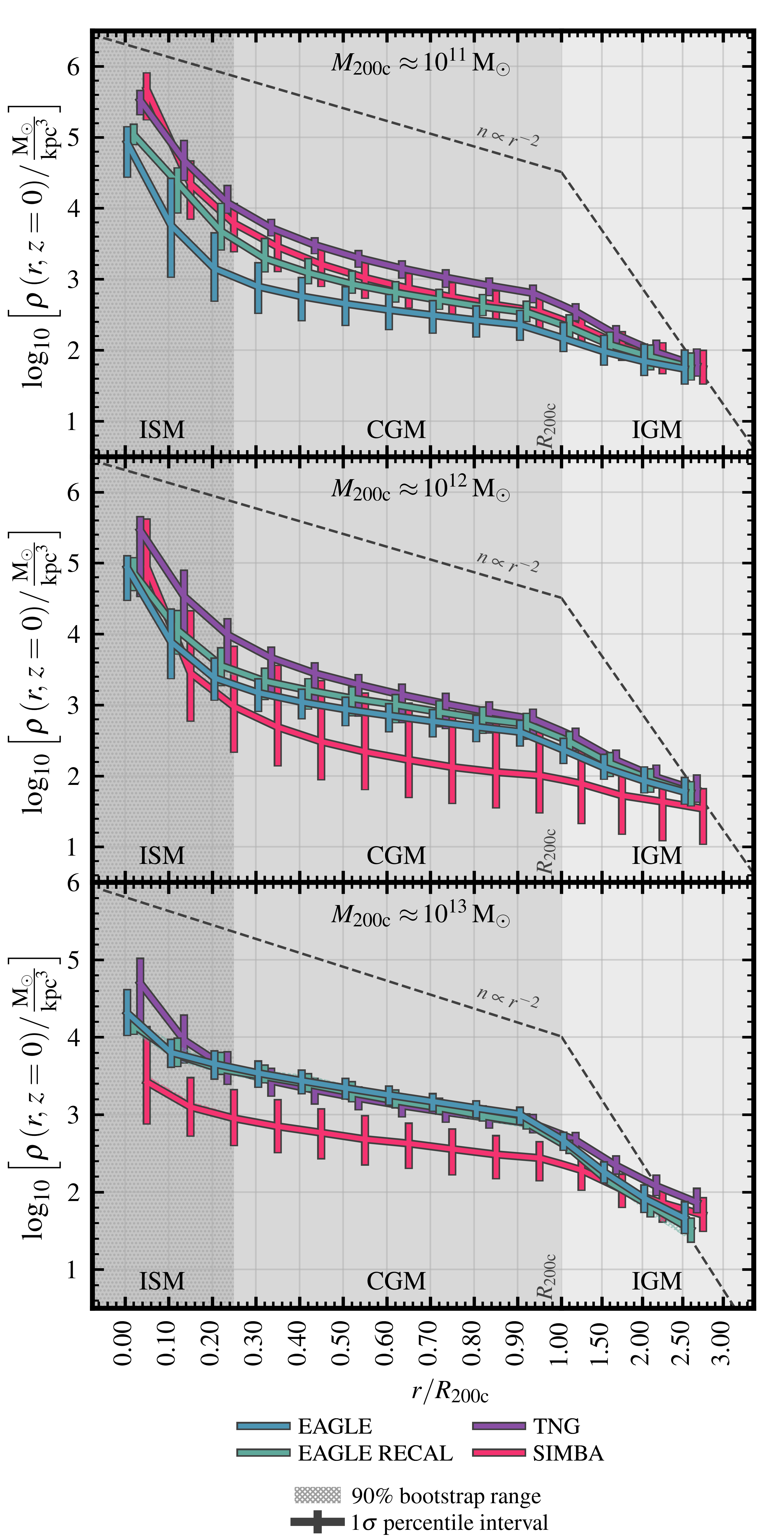
Figure 12: Radial density profiles of galaxies at $z=0$ in EAGLE (blue), EAGLE-RECAL (teal), TNG (purple) and SIMBA (pink). Each row represents a different bin in halo mass, increasing top to bottom. Error-bars correspond to the $16^{\rm th}-84^{\rm th}$ percentile range in inflow rates at a given mass, and hatched regions correspond to the bootstrap-generated $90\%$ confidence interval on the medians at a given mass. Density profiles diverge between the simulations at this redshift, with particularly low densities in EAGLE in the lowest halo mass bin, and SIMBA for the two higher halo mass bins.

Inspecting inflow rates across different scales in TNG, we find that for haloes with $\log_{10}(M_{\rm 200c}/{\rm M}_{\odot})$ $\lesssim 11.5$, inflow rates at the ISM scale ($0.25\times R_{\rm 200c}$) are similar to inflow rates at the halo boundary at $z\approx 2$; but at $z\approx 0$, they are actually twice as high at the scale of the ISM as those recorded at the scale of the halo. With the relatively dense CGM in TNG in this mass range (see Fig. 12, partly contributed to by the build-up of ejected, metal enriched gas in this region which does not leave the halo), we argue that the ISM-scale inflow rates are higher than halo-scale inflow rates due to a combination of efficient recycling of cold gas, and efficient metal cooling of warm CGM gas at this scale. Above $\log_{10}(M_{\rm 200c}/{\rm M}_{\odot})$ $\approx 12.5$, we find the opposite effect – ISM-scale inflow rates are suppressed relative to halo-scale inflow rates (as is true for all simulations in this mass regime).

Lastly, focusing on inflow rates in SIMBA, we find that below $\log_{10}(M_{\rm 200c}/{\rm M}_{\odot})$ $\lesssim 11.5$, accretion rates are suppressed equally at $r=0.25R_{\rm 200c}$, $R_{\rm 200c}$, and $2.5R_{\rm 200c}$. Based on Fig. 4 and 5, this aligns with a scenario where the spatial range of stellar feedback sits between that of EAGLE (far-reaching, beyond the halo) and TNG (within the inner CGM). For $\log_{10}(M_{\rm 200c}/{\rm M}_{\odot})$ $\gtrsim 12$, SIMBA predicts a steadily increasing inflow prevention effect moving inwards from $r=2.5\times R_{\rm 200c}$ to $r=0.25\times R_{\rm 200c}$. Even though the preventative effect is greatest at $0.25\times R_{\rm 200c}$ (with gas inflow rates at just 1-5$\%$ of those expected based on the halo growth rate at $10^{12.5}{\rm M}_{\odot}$), SIMBA predicts that even gas at $2.5\times R_{\rm 200c}$ experiences significant preventative feedback due to AGN. While we do not present the results here, we note that in the SIMBA run with no jet-mode feedback, the preventative effect is greatly reduced – indicating that it is the low-accretion rate, high kinetic energy jet-mode AGN feedback in SIMBA that is responsible for the strong suppression of gas inflow.

To summarise – in EAGLE, TNG and SIMBA, the level of inflow prevention at a given scale can be clearly linked with the presence, or lack thereof, of feedback-driven outflows at the same scale. For $\log_{10}(M_{\rm 200c}/{\rm M}_{\odot})$ $\lesssim 11.5$, EAGLE and SIMBA predict that stellar feedback produces a strong preventative effect on halo-scale inflow rates, while in TNG, halo-scale gas inflow is suppressed by a smaller amount. For halo masses $\log_{10}(M_{\rm 200c}/{\rm M}_{\odot})$ $\gtrsim 12$, SIMBA predicts very strong AGN-driven suppression in halo-scale gas inflow rates, relative to a more mild preventative effect in TNG, and very minimal preventative feedback at the halo scale in EAGLE.

5 Discussion

The EAGLE, TNG, and SIMBA simulations have all been largely successful in producing a reasonable match to the observed galaxy stellar mass function at $z\approx 0$, albeit with careful tuning required to calibrate their respective sub-grid feedback models that cannot be implemented ab initio. We have demonstrated that different implementations of feedback processes – and thus, the manner in which the baryon cycle operates over cosmic time – can be degenerate in producing galaxies at $z\approx 0$ with very similar stellar masses and star formation rates. In §5.1, we use our measurements of gas flows rates across the simulations in §4 to make the causal link between the baryon cycle and static halo properties. In §5.2, we compare our results to previous literature investigating the baryon cycle in simulated galaxies. Lastly, in §5.3 we outline a number of promising observational avenues by which the degeneracy between different feedback models could be broken.

5.1 The influence of gas flows on halo baryon content

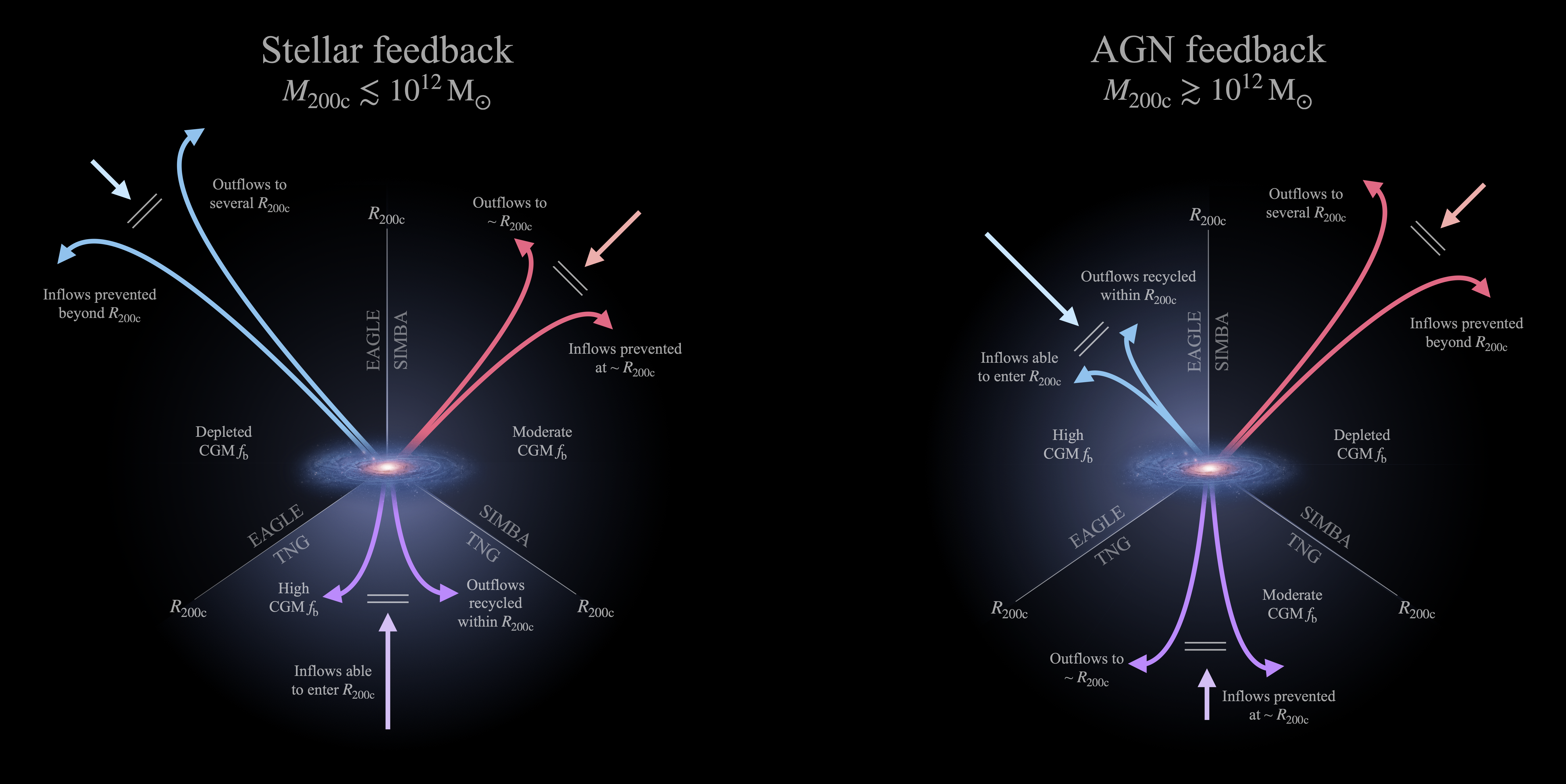
Figure 8: Schematic diagram summarising the different gas flow paradigms found in EAGLE, TNG and SIMBA, split into low mass haloes where stellar feedback dominates (left), and higher mass haloes where AGN feedback dominates (right).

In Figure 8, we summarise the main findings of this study in visual form – indicating the scale reached by feedback-driven outflows in each of the simulations and the consequent gas content of the CGM in each of the simulations. We split this diagram into the low mass ($M_{\rm 200c}\lesssim 10^{12}{\rm M}_{\odot}$) and high mass ($M_{\rm 200c}\gtrsim 10^{12}{\rm M}_{\odot}$) regimes, where stellar and AGN feedback respectively dominate. Our findings in §4 aid in the interpretation of our findings in §3 – in particular Fig. 2 – where we compare the total baryon content of haloes in each simulation, and its breakdown into stellar and gaseous components. Firstly, we discuss the low-mass regime, $\log_{10}(M_{\rm 200c}/{\rm M}_{\odot})$ $\lesssim 12$, where stellar feedback dominates the behaviour of the baryon cycle. In EAGLE, the efficient removal of gas to large scales – where outflows reach several times the virial radius at both $z\approx 2$ and $z\approx 0$ – can be clearly linked with the reduced halo gas content below $\log_{10}(M_{\rm 200c}/{\rm M}_{\odot})$ $\approx 11.5$ in Fig. 2. This is maintained by the reduced halo gas inflow rates as a consequence of direct prevention of cosmological gas accretion, as shown in §4.2.

In contrast, in TNG, stellar feedback driven outflows typically stall before reaching $R_{\rm 200c}$. This deposits a significant amount of enriched gas in the CGM that can subsequently be efficiently recycled into the ISM, resulting in increased ISM-scale inflow rates relative to even halo-scale inflow in TNG at $z\approx 0$. This efficient intra-halo recycling scenario means that in low-mass haloes, the baryon content of the CGM in TNG is much higher than that recorded in EAGLE at $z\approx 0$. SIMBA predicts a picture in between that of EAGLE and TNG, where some gas is fully removed from the halo via stellar feedback (particularly below $\log_{10}(M_{\rm 200c}/{\rm M}_{\odot})$ $\approx 11$), and some portion of these outflows stall within the CGM. This leads to halo-wide baryon fractions and CGM gas content between that of EAGLE and TNG at $z\approx 0$.

Next, we discuss the high-mass regime – $\log_{10}(M_{\rm 200c}/{\rm M}_{\odot})$ $\gtrsim 12$ – where AGN feedback becomes dominant in these simulations, and plays a driving role in the baryon cycle. In EAGLE, we find that the purely thermal implementation of AGN feedback can remove gas from the ISM, but is seldom powerful enough to remove gas to large scales and significantly influence cosmological inflow. This is likely a consequence of rapid thermal dissipation as the gas travels through the CGM, meaning that the outflows stall before travelling far beyond the halo. Even so, this thermal energy (in combination with the transition to a hot, virialised halo atmosphere – e.g. Correa et al. 2018a, b) is sufficient to prevent cosmological inflow from entering the ISM (see Fig. 6 and 7), and ultimately curtail star formation rates in high mass galaxies. Since little gas is expelled from the halo and the preventative impact of AGN works within the CGM, this leads to the result shown in Fig. 2 where galaxy baryon fractions monotonically increase with halo mass.

In §4, we show in Fig. 4 and 5 that AGN-driven outflows in TNG and SIMBA reach much larger scales before stalling, presumably because of the kinetic implementation of feedback in the "jet mode" in both models. At $z\approx 0$ we show that for haloes with $\log_{10}(M_{\rm 200c}/{\rm M}_{\odot})$ $\approx 12.5$, gas outflow rates at $2.5\times R_{\rm 200c}$ are just as high as they are at $R_{\rm 200c}$ in TNG, and even higher in the case of SIMBA. Unlike in EAGLE (where the preventative effect of AGN is confined to within the CGM), these outflows also act to prevent cosmological gas accretion at the halo-scale. Together, particularly in the case of SIMBA, this causes the downturn in halo baryon fractions at intermediate halo mass which we demonstrate in Fig. 2.

5.2 Comparison to previous literature

In this section, we outline how our results compare with previous theoretical studies relating to the baryon cycle of galaxies. In particular, we focus on comparing how outflow and inflow rates change with scale relative to the simulations we study here.

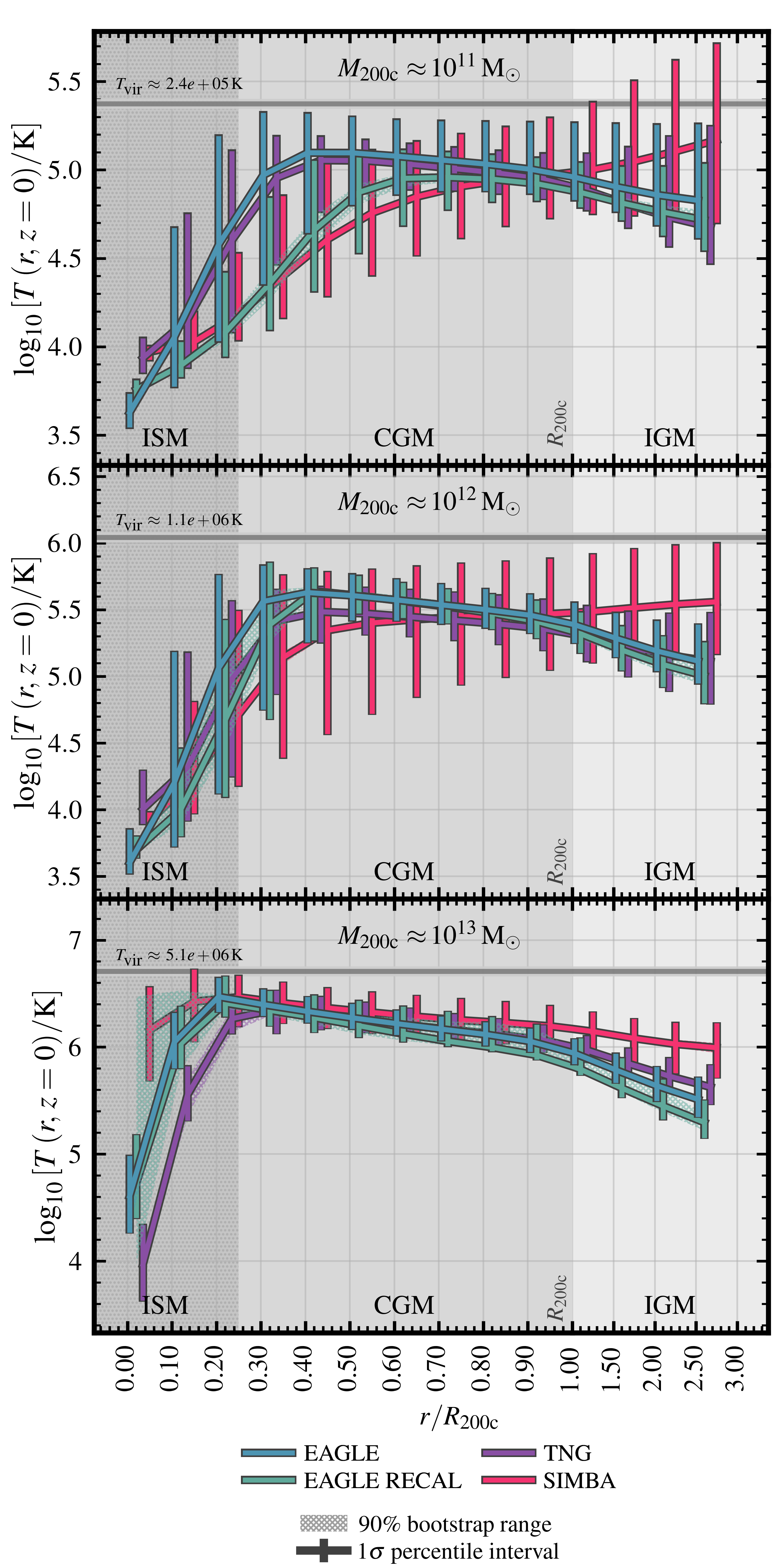
Figure 14: Radial temperature profiles of galaxies at $z=0$ in EAGLE (blue), EAGLE-RECAL (teal), TNG (purple) and SIMBA (pink). Each row represents a different bin in halo mass, increasing top to bottom. Error-bars correspond to the $16^{\rm th}-84^{\rm th}$ percentile range in inflow rates at a given mass, and hatched regions correspond to the bootstrap-generated $90\%$ confidence interval on the medians at a given mass. Temperature profiles are in slightly better agreement between the simulations compared to $z\approx 2$, with generally hotter CGM.

As outlined in §2.2 and Appendix A, we have demonstrated that our methodology for measuring gas flow rates produces results that are consistent with previous studies utilising the EAGLE simulations (Mitchell et al., 2020) and the TNG suite (Nelson et al., 2019). Fig. 14 in Mitchell et al. (2020) shows the difference between $z\approx 2$ outflow mass loading reported by Nelson et al. (2019) in the TNG50 simulations, compared with those measured in EAGLE. For galaxies with stellar mass below $\approx 10^{10}{\rm M}_{\odot}$, where stellar feedback is efficient, gas outflow rates in TNG50 tend to decrease from smaller ($20\,{\rm kpc}$) to larger ($50\,{\rm kpc}$) radii. Comparatively, in EAGLE  the mass loading is identical at both of these scales. Our work, which uniquely applies a like-for-like methodology to measure gas flow rates between the simulations, provides a comprehensive explanation for this result – showing that SF-driven outflows produce a larger-scale impact on the baryon cycle in EAGLE compared to TNG.

We can also compare our results with those from zoom-in simulations, where improvements in resolution enable more detailed sub-grid modelling for gas cooling, star formation and feedback within the ISM. Muratov et al. (2015) and Anglés-Alcázar et al. (2017b) investigate mass loading and baryon cycle predictions from the FIRE simulations, introduced in Hopkins et al. (2014). FIRE implements stellar feedback by injecting energy, momentum, mass, and metals from stellar radiation pressure, Hii photo-ionization and photo-electric heating, Type I and Type II supernovae, and stellar winds – while not hydrodynamically decoupling or disabling cooling for affected gas elements. The $M_{\star}-\eta$ relations presented in Muratov et al. (2015) and Anglés-Alcázar et al. (2017b) (with an Eulerian, shell-based technique and Lagrangian, particle tracking technique respectively) are very similar to those we present for SIMBA in Fig. 3. This is, perhaps, unsurprising, given that SIMBA uses the FIRE power-law fits as the prescriptive mass loading factor and wind velocity. The mass loading values at fixed stellar mass in TNG and EAGLE are, thus, lower than the predictions from FIRE (for the mass range considered here, $M_{\star}\gtrsim 10^{9}{\rm M}_{\odot}$).

Focusing on an individual system (m12i), Muratov et al. (2015) show that in a halo with $M_{\rm 200c}\approx 10^{12}{\rm M}_{\odot}$ at $z\approx 2$, mass loading values at the ISM scale ($0.25\times R_{\rm 200c}$) are stochastic (like the outflows themselves), however typically take a value of $\eta\approx 10^{1}$ in episodes of star formation. In this same system, Muratov et al. (2015) show that outflow rates at $R_{\rm 200c}$ reach only $\approx 10-20\%$ of the outflow rate at the ISM in episodes of star formation. This aligns with the predictions we outline from TNG and SIMBA, where SF-driven outflows typically recycle within the CGM at this mass scale. Comparatively, in EAGLE, mass flow rates at both radii are very similar at $z\approx 2$ (on average).

Pandya et al. (2021) investigate the mass, momentum, and energy loading in the subsequent FIRE-2 simulations (Hopkins et al., 2018). When using the same radial shell to define the ISM and no minimum outgoing velocity requirement (as per the method in Muratov et al. 2015), they find a very similar mass loading scaling with stellar mass. At $z\approx 0$ in a halo of mass $M_{\rm 200c}\approx 10^{12}{\rm M}_{\odot}$ (m12f), they show that halo-scale gas outflow rates rarely exceed those from the ISM escape – again, in alignment with the picture painted by TNG and SIMBA at this mass. Interestingly, for dwarf haloes with $M_{\rm 200c}\approx 10^{10}{\rm M}_{\odot}$, Pandya et al. (2021) find that mass outflow rates at the halo scale nominally exceed that measured at the ISM scale, and at $M_{\rm 200c}\approx 10^{11}{\rm M}_{\odot}$, that outflow rates at the two scales can be roughly equal (if the time delay as the outflow traverses the ISM is taken into account). The former case is similar to the picture painted by EAGLE at $M_{\rm 200c}\approx 10^{11}{\rm M}_{\odot}$, where mass is entrained in outflows through the CGM. This indicates that in FIRE-2, the scale reached by outflows is strongly influenced by halo mass.

Christensen et al. (2016) use a particle-tracking technique to study gas flows in and around galaxies in a suite of gasoline-based simulations (Wadsley et al., 2004). These simulations use a “blast-wave” technique (where cooling is temporarily disabled) to distribute energy from stellar feedback, as per Stinson et al. (2006). As demonstrated in Mitchell et al. (2020), Christensen et al. (2016) find lower ISM-scale mass loading factors than those measured in EAGLE, and a steeper decline in $\eta$ with mass. Since the ISM-scale mass loading values are lowest in EAGLE of the 3 simulations we discuss here (see Fig. 3), this indicates that the mass loading values in Christensen et al. (2016) are also lower than measured in SIMBA and TNG. While direct measurements of halo-scale outflow rates are not presented, they find that a substantial fraction of the gas that leaves the ISM will also leave the halo virial radius.

Tollet et al. (2019) present an analysis of gas flows in the NIHAO simulations using a Lagrangian particle tracking method (Wang et al., 2015). NIHAO also uses the blast-wave technique to distribute energy from stellar feedback, as per Stinson et al. (2006). As a function of stellar mass, mass loading values in NIHAO are similar to TNG and SIMBA at $M_{\star}\approx 10^{9}{\rm M}_{\odot}$ ($\eta\approx 10^{1.5}$), however decrease sharply with stellar mass to $\eta\approx 10^{-0.5}$ at $M_{\star}\approx 10^{10.5}{\rm M}_{\odot}$. At the same stellar mass, predictions from EAGLE, TNG, and SIMBA are one full decade higher at $\eta\approx 10^{0.5}$. For haloes with $M_{\rm 200c}\lesssim 10^{12}{\rm M}_{\odot}$, they show that the majority of gas does not exit $R_{\rm 200c}$ after being ejected from the ISM.

The total baryon fraction of haloes within $R_{\rm 200c}$ we measure align with the findings presented in Ayromlou et al. (2023), who also analyse the EAGLE, TNG, and SIMBA simulations to show how feedback redistributes the baryons in and around haloes. This is measured in terms of the “closure radius” of haloes – the minimum radius at which the enclosed baryon content reaches the universal value. They find that for low mass haloes where stellar feedback dominates ($M_{\rm 200c}\lesssim 10^{11.5}{\rm M}_{\odot}$), the closure radius is the largest for EAGLE galaxies, followed by SIMBA galaxies, and then TNG galaxies. In the case of higher mass haloes where AGN feedback dominates ($M_{\rm 200c}\gtrsim 10^{12}{\rm M}_{\odot}$), the closure radius is the largest for SIMBA galaxies, followed by TNG galaxies, and then EAGLE galaxies.

Our findings also provide insight into the measurements presented in Davé et al. (2020), who investigate the global cool gas (${\rm H}$i and ${\rm H}_{2}$; decomposed in post-processing) content of galaxies in the same simulations and compare with available observations. At $z\approx 0$, Davé et al. (2020) show that the fiducial resolution EAGLE run under-predicts the ${\rm H}$i content of galaxies compared to local ALFALFA observations of the ${\rm H}$i-MF (Jones et al., 2018), as well as the ${\rm H}$i fraction of galaxies as a function of $M_{\star}$. Given that the ${\rm H}$i identified by this decomposition algorithm tends to trace the gas that is slightly more diffuse and extended than ${\rm H}_{2}$ gas, the low ${\rm H}$i content of EAGLE galaxies could be explained by the stellar feedback scenario we outline above, which evacuates much of the CGM – and, likely, some of the gas identified as ${\rm H}$i which resides the edge of the ISM. We do note, however, that predictions from the recalibrated, higher resolution EAGLE run and ${\rm H}$i observations and are in closer agreement (see also Fig. 11 and 12).

Our results highlight the fact that differences in baryon cycling can indeed leave signatures even at the scale of the ISM, particularly when considering multi-phase gas. With the resolution and physics improvements in the next generation of cosmological simulations, it will become possible to better resolve the phase structure of the ISM in a self-consistent manner – and thus, to produce statistical predictions for the spatially resolved properties of the ISM, as well as the influence of gas flows on these distributions. Such advancements will also provide the statistical context necessary to generalise the results of high-resolution zoom simulations (some of which we summarise above), which provide more detailed insight into the link between the ISM and CGM.

5.3 Identifying observational feedback tests

As discussed in §1, direct observation and quantification of the gas flows surrounding galaxies is very challenging – particularly when seeking to compare the baryon cycle at a statistical level. This means that currently, it is very difficult to place constraints on which feedback scenarios are favoured by observations. Here, we briefly outline some avenues against which these models could be tested with current and/or future observations.

Comparing the average gas density profiles between simulations at $z\approx 2$ and $z\approx 0$ in Fig. 11 and 12, it is clear that the differences in total halo gas content arising from disparate baryon cycling paradigms are clearest at $z\approx 0$, after the variability between models has had adequate time to consolidate in terms of static halo properties. Presently, a combination of X-ray observations and weak lensing studies have been able to place constraints on the gas fraction of high-mass galaxy groups and clusters ($M_{\rm 500c}\gtrsim 10^{13}\,{\rm M}_{\odot}$, e.g. Hoekstra et al. 2015; Pearson et al. 2017; Mulroy et al. 2019; Lovisari et al. 2020; Akino et al. 2022); which can be used to calibrate the strength of AGN feedback in the next generation of cosmological hydrodynamical models (e.g Schaye et al. 2023; Kugel et al. 2023). As demonstrated in Figure 2, such observations indicate that the baryon fractions of haloes of mass $M_{\rm 500c}\approx 10^{14}\,{\rm M}_{\odot}$ within $R_{\rm 500c}$ are slightly too high in EAGLE and TNG (very close to the universal value), and slightly too low in SIMBA.

As demonstrated in Fig. 2, the most significant AGN-driven difference in halo baryon content is induced below the mass scale of clusters, between $M_{\rm 200c}\approx 10^{12}-10^{13}\,{\rm M}_{\odot}$. Measurements of the baryon content of haloes in this mass range would provide significant constraining power on the strength of AGN feedback, as well as the mass scale at which SMBH accretion and feedback becomes efficient. Preliminary studies using the eROSITA telescope (Predehl et al., 2021) and stacked soft X-ray observations indicate that for galaxies with stellar mass $M_{\star}\approx 10^{11}\,{\rm M}_{\odot}$, forward-modelled X-ray luminosity profiles (up to $\approx R_{\rm 200c}$) from EAGLE and TNG are consistent with observational constraints (Oppenheimer et al., 2020; Chadayammuri et al., 2022). Further constraints on the baryon fraction of haloes in this mass range will become possible with observations utilising the Sunyaev Zeldovich (SZ) effect – for instance, Bregman et al. (2022) demonstrate the feasibility of placing such constraints in a small sample of local $\approx L^{*}$ haloes. Yang et al. (2022) demonstrate that the disparate baryon content of haloes between TNG and SIMBA above $\log_{10}(M_{\rm 200c}/{\rm M}_{\odot})$ $\approx 12.5$ produces an observationally detectable difference in forward-modelled SZ measurements, provided that an instrument with adequate angular resolution is utilised (such as the upcoming Simons Observatory, Ade et al. 2019). In this mass range, studies investigating the ${\rm H}$i content of groups using stacking techniques may also prove useful to constraining baryon content (e.g. Dev et al. 2023), particularly with radio surveys such as DINGO with the ASKAP telescope (Hotan et al., 2021) and MIGHTEE-HI with MeerKAT (Maddox et al., 2021).

Below mass scales of $M_{\rm 200c}\approx 10^{12}\,{\rm M}_{\odot}$, it is very difficult to observationally constrain the baryon content of galaxies and their CGM. In this mass range, the CGM is expected to be multi-phase and anisotropic (e.g. McCourt et al. 2018; Fielding et al. 2020), constituted of a combination of cool filamentary inflow structures together with enriched recycling gas. Observations have shown that sight-line measurements of CGM metallicity can vary by up to ${\rm 2}\,{\rm dex}$ within the same halo (e.g. Lehner et al. 2013; Prochaska et al. 2017; Zahedy et al. 2019). The resolution of the cosmological hydrodynamical simulations we study here is inadequate to resolve detailed phase structure, and more detailed sub-grid models are also likely required to accurately model the CGM (e.g. Crain & van de Voort, 2023). We can, however, make general comments regarding the expected impact of different feedback regimes on the properties of the CGM.

In the case of EAGLE, where the CGM is predicted to be nearly entirely devoid of gas at low halo masses, Wright et al. (2021) show that the integrated metallicity of the CGM is extremely sensitive to the rate of pristine halo-scale gas accretion. This is a result of newly introduced gas being able to efficiently dilute the metallicity of the already small gaseous reservoir, which is only possible due to the previous evacuation of the CGM via far-reaching, strong stellar feedback. Thus, in a model like EAGLE, we might expect to find significant amounts of very metal poor to pristine gas in the CGM, which would not be the case in a model like TNG where the metal-enriched gas from SF-driven outflows is directly deposited into the CGM. Despite this, we refrain from comparing the models in terms of the distribution of metals in the CGM in this work, as it is non-trivial to disentangle differences in the modelling of metal diffusion (included in TNG, but not in EAGLE or SIMBA) from changes induced by differences in gas flows.

In any case, it is clear that the scale and strength of stellar feedback will leave signatures in the distribution of metals in the CGM. Péroux et al. (2020) demonstrate that TNG and EAGLE predict similar net gas flows rates as a function of galacto-centric azimuthal angle for galaxies with $M_{\star}\approx 10^{9.5}\,{\rm M}_{\odot}$ and $M_{\star}\approx 10^{10.5}\,{\rm M}_{\odot}$. Investigating the scale of metal-enrichment at different impact parameters, particularly studying how angular and radial variations would manifest in discrete sight-line observations, could constitute a promising test of model accuracy. This is potentially possible with carefully constructed comparisons with current surveys that probe different phases of the CGM, such as COS-Halos (Tumlinson et al., 2013; Werk et al., 2014; Prochaska et al., 2017) and MEGAFLOW (Schroetter et al., 2016; Zabl et al., 2019).

Alone this line, DeFelippis et al. (2021) compare results from the MEGAFLOW survey with predictions from the TNG50 simulation (several fold higher resolution than the TNG100 simulation we investigate here, but the same feedback physics); indicating that TNG50 can reasonably reproduce observations of the kinematic diversity of strong MgII absorbers (tracing the cool CGM) in the halo mass range $10^{11.5}\,{\rm M}_{\odot}-10^{12}\,{\rm M}_{\odot}$. Appleby et al. (2021) compare results from SIMBA and the COS-Halos and COS-Dwarfs survey, finding general agreement with observations regarding the predicted abundance of ${\rm H}$i and metal absorbers in the CGM of star-forming SIMBA galaxies, but find slight tension in the quenched population. Appleby et al. (2023) also demonstrate the feasibility of using machine learning to infer CGM conditions from absorption line properties, finding that their model trained on SIMBA can accurately predict absorber overdensity, temperature, and metallicities.

The Habitable Worlds Observatory, a large space based UV-optical-IR mission concept endorsed by the US Astro2020 Decadal report, will provide greatly enhanced spectroscopic sensitivity in the UV relative to the HST Cosmic Origins Spectrograph, enabling significantly larger samples of $z\lesssim 1$ galaxies with absorption line studies of their CGM (NAS, 2021). Furthermore, new ways of probing the CGM continue to be proposed and tested – for instance using fast radio bursts (FRBs; Macquart et al. 2020), and the characterisation of of Ly$\alpha$ haloes in both emission (e.g. Lokhorst et al. 2019; Augustin et al. 2019) and absorption (i.e. Ly$\alpha$ forest, see Tillman et al. 2023a, b).

Observations of gas flow rates – as opposed to static measurements of halo baryon content – will also prove useful in constraining feedback models in simulations. Different techniques can provide measurements on the multi-phase nature of galactic outflows in individual systems; for instance CO tracing cool molecular outflows (e.g. Leroy et al. 2015 using ALMA observations), or with metal absorption lines and detailed ionisation modelling (e.g. see discussions in Chisholm et al. 2016; Veilleux et al. 2020). Combining careful forward-modelling from simulations with observational approaches across wavelength may be able to place constraints on total gas outflow rates as the sample size of outflow measurements continues to grow.

6 Summary

In this paper, we have conducted a like-for-like comparison of the baryon cycle in three modern cosmological hydrodynamical simulations: EAGLE, TNG, and SIMBA. We use a common methodology to analyse the gas flows in and around central galaxies, from the scale of the ISM to several halo virial radii. While galaxies in these simulations share very similar stellar mass content and star-formation rates at $z\approx 0$, our work has highlighted that this agreement is achieved for very different physical reasons.

Concerning haloes with mass $M_{\rm 200c}\lesssim 10^{11.5}{\rm M}_{\odot}$, where stellar feedback is dominant, we summarise our results as follows:

• In EAGLE, SF-driven outflows are able to reach several times $R_{\rm 200c}$ before stalling. At $z\approx 0$, mass outflow rates increase with scale with the gas surrounding galaxies being very tenuous and under-pressurised relative to the outflows. At $z\approx 2$ we do not see mass entrainment in outflows with increasing scale, where the CGM is still relatively dense and more cool/filamentary in nature.

• The extended scale of SF-driven outflows in EAGLE leads to a significant preventative effect on gas inflow at the halo-scale.

  Overall, this leads to haloes with a low density CGM and very low baryon fractions (just 10% of the cosmological value) in this mass range at $z\approx 0$.

• In TNG, SF-driven outflows are very strong at the scale of the ISM, however, tend to stall within the CGM before reaching $R_{\rm 200c}$. This is also true in SIMBA at $z\approx 2$, however at $z\approx 0$, SF-driven outflows in SIMBA can reach a similar scale as in EAGLE (albeit without mass entrainment).

• In TNG, halo baryon fractions remain above 50% of the cosmological value in this mass regime at $z\approx 0$. SF-driven outflows are recycled within the scale of the halo, with inflow rates at the ISM-scale higher than at the halo-scale due to very efficient cooling within the dense, enriched CGM.

• In SIMBA, halo baryon fractions in this mass regime are between those measured in EAGLE and TNG, reflecting moderate preventative feedback on halo-scale gas inflows.

Furthermore, in relation to haloes with mass $M_{\rm 200c}\gtrsim 10^{12}{\rm M}_{\odot}$, where AGN feedback is dominant:

• In EAGLE, AGN-driven outflows do not reach far beyond $R_{\rm 200c}$ at either $z\approx 0$ nor $z\approx 2$. This leads to minimal preventative impact on gas inflow at the halo scale, but significantly prevents gas inflow at the scale of the ISM.

• In TNG, AGN-driven outflows are more powerful than in EAGLE, with at least some gas in these outflows reaching $2-3\times R_{\rm 200c}$. This leads to a moderate preventative impact on cosmological inflow at the halo-scale, with further inflow prevention within the heated CGM. As a result, there is a significant turnover in halo baryon fractions at $z\approx 0$, reaching values as low as 50% of the cosmological value at $M_{\rm 200c}\approx 10^{12.5}\,{\rm M}_{\odot}$.

• In SIMBA, AGN-driven outflows are significantly stronger than in both EAGLE and TNG, particularly at $z\approx 0$. These outflows continually entrain mass from the ISM scale to several times $R_{\rm 200c}$. This causes a very significant drop in halo-scale cosmological gas inflow, and a corresponding drop in halo baryon fractions to as low as 20% of the universal value between $M_{\rm 200c}=10^{12}{\rm M}_{\odot}-10^{13}{\rm M}_{\odot}$.

This work lays the foundation for developing targeted observational tests that can favour or disfavour certain feedback scenarios, and move towards a more constrained understanding of the role of feedback processes in the baryon cycle. Such an understanding will be imperative to inform the next generation of cosmological simulations, and to maximise their scientific utility. Additionally, a precise understanding of the baryonic effects on the large-scale matter distribution (see Delgado et al. 2023; Gebhardt et al. 2023) will be imperative in order to extract meaningful constraints from future weak lensing studies with regard to cosmological parameters, cosmic shear, and the growth of cosmic structure.

Data Availability

The EAGLE (http://icc.dur.ac.uk/Eagle/), TNG (https://www.tng-project.org/), and SIMBA (http://simba.roe.ac.uk/) simulation outputs used for our analysis are all publicly available. All of the measurements presented in this paper are produced based on the methodology outlined in §2.2, and are extracted using like-for-like techniques between each of the simulations. The gas flow catalogs generated for this work will be shared by the corresponding author upon reasonable request.

Appendix A Comparison of gas flow measurements with previous literature

In this section, we compare our measurements of gas flow rates with those measured from the same simulations (where applicable) in previous literature. As outlined in §2.2, we elect to use an Eulerian or “instantaneous” approach to calculating gas flow rates, rather than a Lagrangian particle tracking method.

Figure 9 shows a comparison of $z\approx 2$ and $z\approx 0$ halo-scale mass loading factors at the ISM scale (here, $0.20\times R_{\rm 200c}$) in EAGLE as a function of $M_{\rm 200c}$ mass. While Mitchell et al. (2020) take a Lagrangian particle-tracking approach to measure gas flow rates, we recover good agreement with their results (to within $\approx 0.2\,$dex across the halo mass range). Our instantaneously measured mass loading factors are systematically (very) slightly higher than the Mitchell et al. (2020) results, likely due to the latter not including the subset of gas that is very quickly recycled within the $\Delta t$ used for the Lagrangian calculation. This offset is highest at $M_{\rm 200c}\approx 10^{13}{\rm M}_{\odot}$, indicating that some AGN-driven outflows in EAGLE may be recycled quite quickly at the ISM scale.

Figure 10 shows a comparison of $z\approx 2$ $10{\rm kpc}$-scale mass loading factors as a function of $M_{\star}$ in TNG for two different choices of outflow velocity cut: $50\,{\rm km\,s^{-1}}$, and $150\,{\rm km\,s^{-1}}$. Utilising a very similar method, our measurements agree very well, to within $\approx 0.1\,{\rm dex}$ for both velocity thresholds, across the range of stellar masses shown. As discussed in §2.2, in the main body of this paper we do not enforce a minimum velocity threshold for the outflows. With experimentation, we find that imposing a velocity threshold does not qualitatively influence our results.

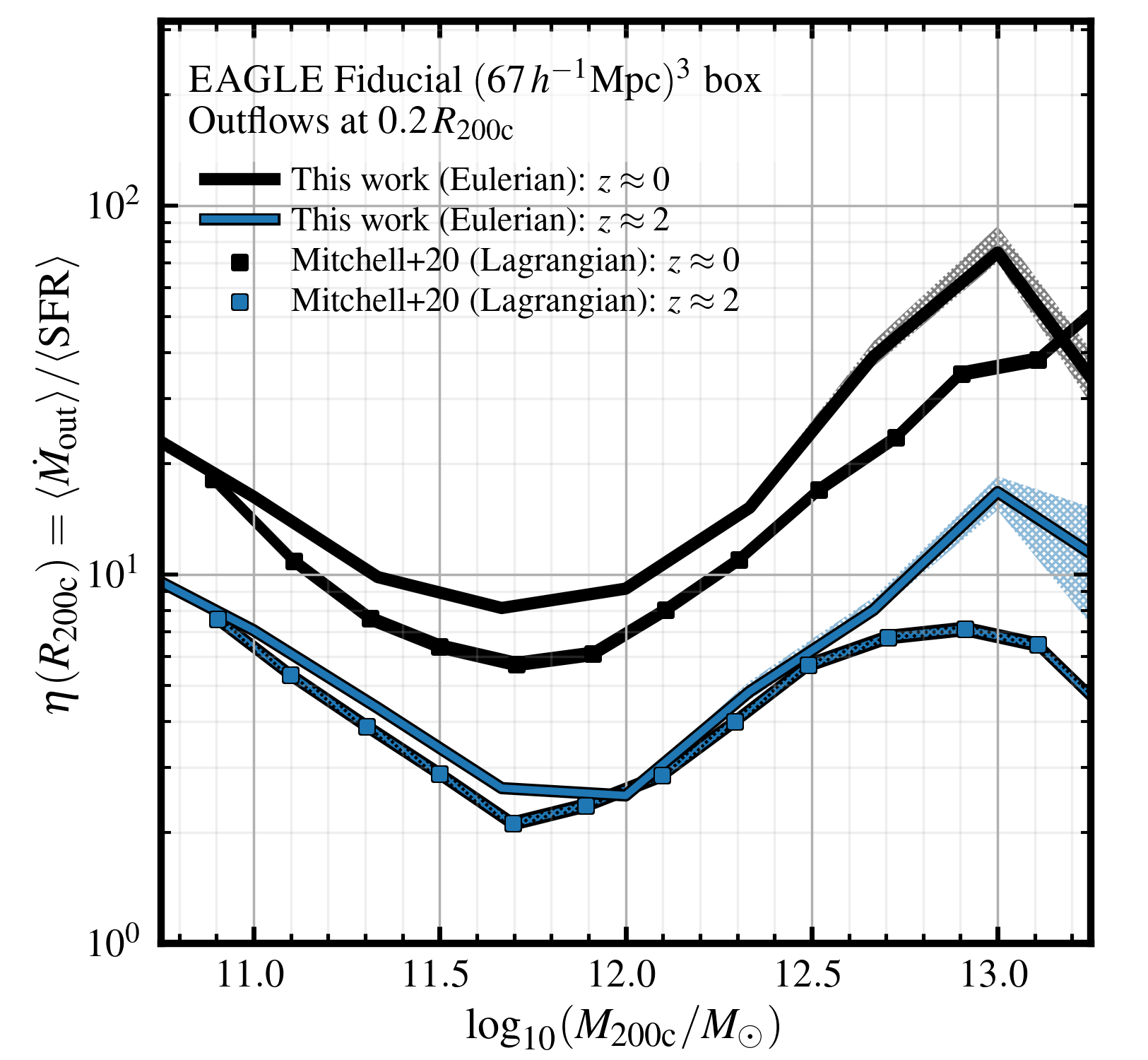
Figure 9: Comparison of $z\approx 2$ (blue) and $z\approx 0$ (black) halo-scale mass loading factors ($\eta\equiv\langle\dot{M}_{\rm out}\rangle/\langle\dot{M}_{\star}\rangle$) as a function of $M_{\rm 200c}$ mass measured in this work (solid lines, no shading), and the measurements presented in Mitchell et al. (2020) (square markers connected with dot-filled solid lines). In our calculations, hatched shaded regions correspond to the bootstrap-generated $90\%$ confidence interval on the medians at a given mass. At both redshifts, our measurements agree well, to within $\approx 0.2\,{\rm dex}$.

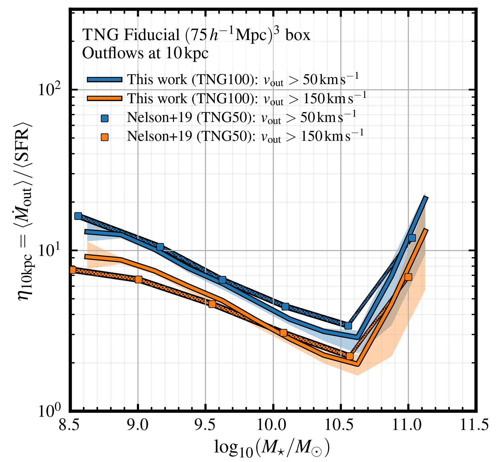
Figure 10: Comparison of $z\approx 2$ mass loading factors ($\eta\equiv\langle\dot{M}_{\rm out}\rangle/\langle\dot{M}_{\star}\rangle$) at $10\,{\rm kpc}$ measured in this work (solid lines, no shading) and those presented in Nelson et al. (2019) (square markers connected with dot-filled solid lines). The data presented in orange correspond to outflow measurements with a minimum outflow velocity of $150\,{\rm km\,s^{-1}}$, while the data presented in blue correspond to outflow measurements with a minimum outflow velocity of $50\,{\rm km\,s^{-1}}$. In our calculations, hatched shaded regions correspond to the bootstrap-generated $90\%$ confidence interval on the medians at a given mass. For both velocity thresholds, our measurements agree very well, to within $\approx 0.1\,{\rm dex}$.

Appendix B Galaxy density profiles

In Fig. 11 and 12, we show the density profiles of galaxies in each of the simulations at $z=2$ and $z=0$ respectively. Each row represents a different bin in halo mass – top: $\log_{10}(M_{\rm 200c}/{\rm M}_{\odot})$ $\in[10.75,11.25]$; middle: $\log_{10}(M_{\rm 200c}/{\rm M}_{\odot})$ $\in[11.75,12.25]$; bottom: $\log_{10}(M_{\rm 200c}/{\rm M}_{\odot})$ $\in[12.75,13.25]$). Radial $x$-values are quoted as fractions of $R_{\rm 200c}$, with a broken scale above $1\times R_{\rm 200c}$ to include radial bins up to $3\times R_{\rm 200c}$. For reference, in each panel we include a dashed line indicating the expected outer slope of an isothermal $\beta$ profile with $\beta=2/3$; i.e. $\rho(r)\propto r^{-2}$.

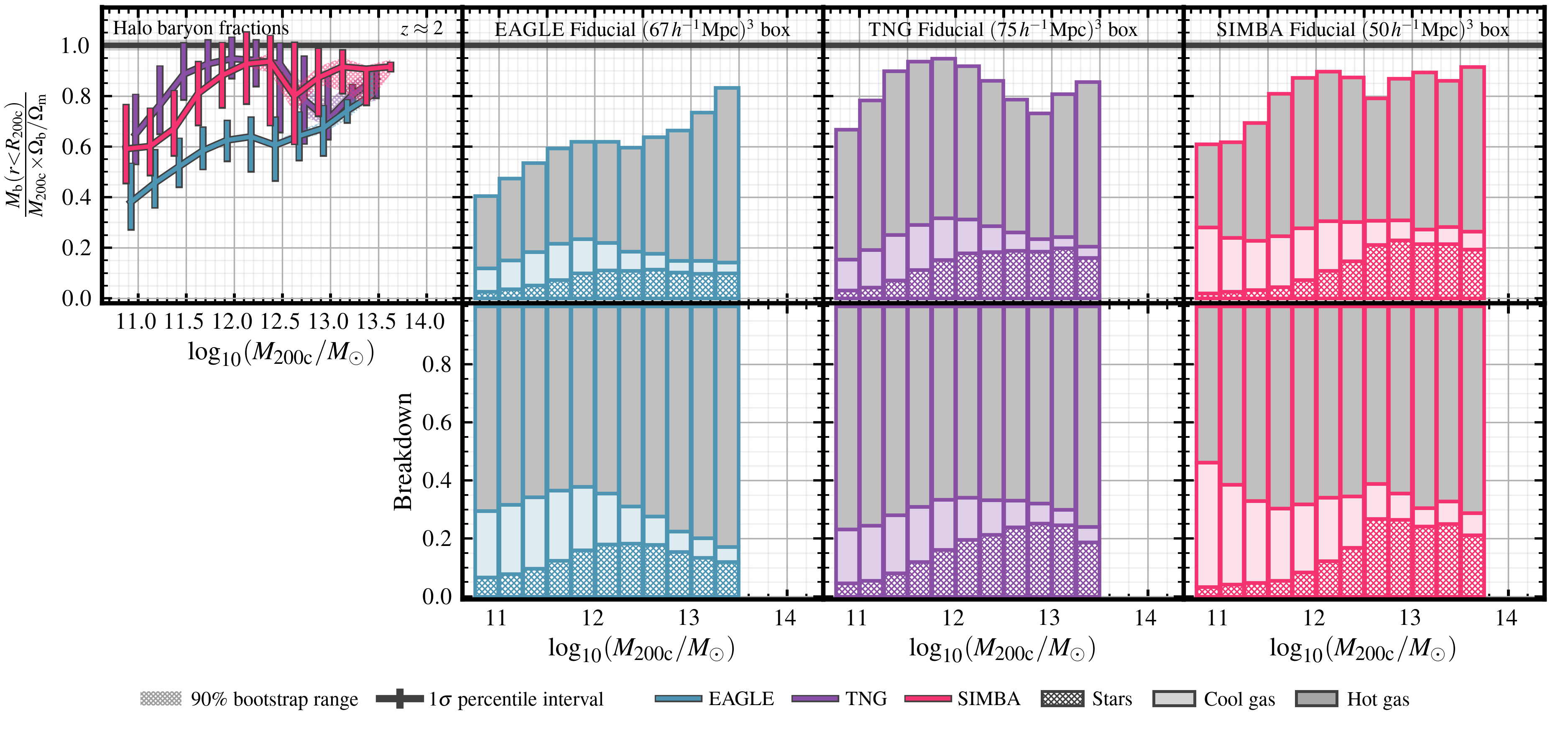
Figure 15: The baryon content of haloes at $z\approx 2$ in EAGLE (blue), TNG (purple) and SIMBA (pink). Top panel, $1^{\rm st}$ column: The median total baryon fraction within $R_{\rm 200c}$ (stars, gas, black holes) of haloes as a function of $M_{\rm 200c}$ mass. Top panels, $2^{\rm nd}-4^{\rm th}$ columns: Total baryon content for each simulation within $R_{\rm 200c}$ broken down into stars (hatched bars), “cool” gas (coloured shaded bars), and “hot gas” (grey bars) in each simulation. In the top panels, this baryon content is normalised by $f_{\rm b}\times M_{\rm 200c}$. Bottom panels: The bottom row of panels shows the same breakdown, but re-normalised by the actual baryonic mass in each halo, $M_{\rm bar}(r<R_{\rm 200c})$. In each of the simulations in the left-hand panel, error-bars represent the $16^{\rm th}-84{\rm th}$ percentiles in halo baryon fractions for a given mass bin; the hatched regions represent the $90\%$ confidence interval on the median from 100 bootstrap re-samplings in each bin. The difference between the simulations in terms of $z\approx 2$ baryon fractions are qualitatively similar compared to that shown at $z\approx 0$ in Fig. 2, but the baryon content of haloes is universally higher.

In general, density profiles at $z=2$ agree fairly well between the simulations. This corresponds to the universally higher baryon content of galaxies and their CGM at this redshift, as demonstrated in Fig. 15. Considering the lowest mass bin at $z=0$, we note that the density of the CGM in EAGLE is quite low – $\approx 1\,{\rm dex}$ lower than the predictions from TNG and SIMBA at the edge of the ISM. This low density allows for the entrainment of gas with outflows in EAGLE, with the outflows being overpressurised relative to the surrounding medium. We observe a similar effect in SIMBA in the two higher mass bins, with CGM densities in the intermediate halo mass bin being $\approx 1\,{\rm dex}$ lower than the predictions from EAGLE and TNG. This signifies the efficient evacuation of the CGM via AGN feedback, which also allows subsequent outflows to be overpressurised relative to the CGM and entrain gas in the outflows towards larger scales.

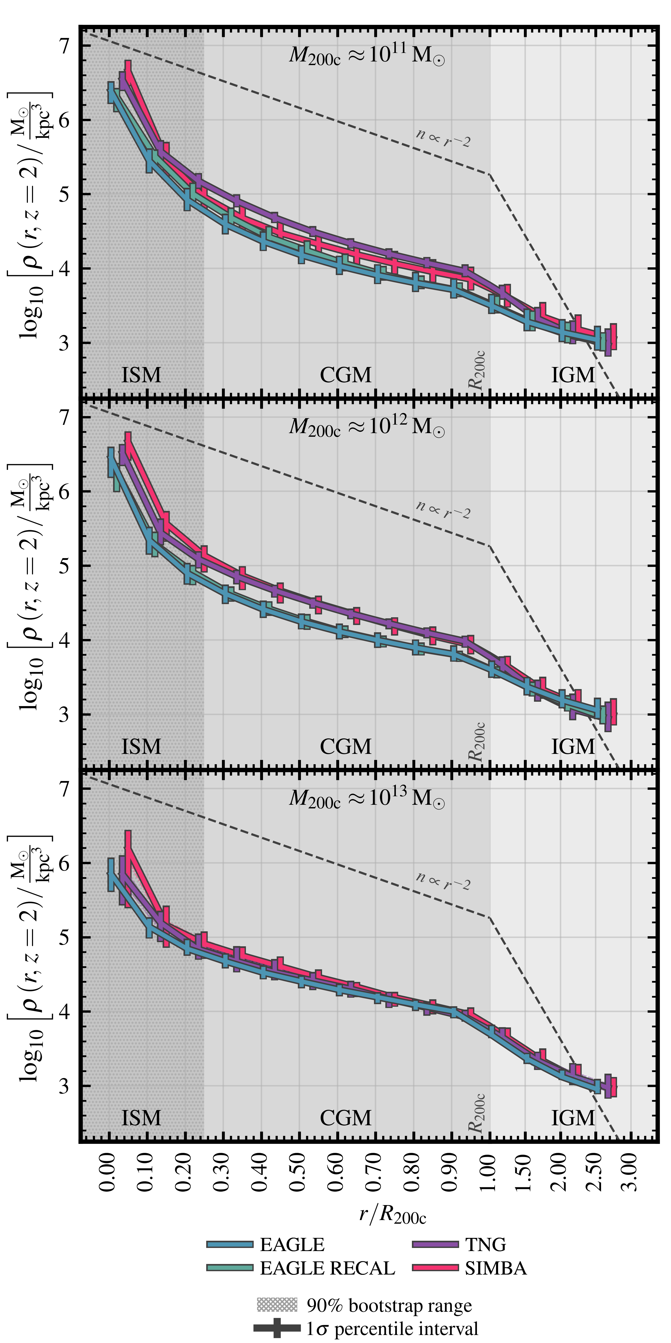
Figure 11: Radial density profiles of galaxies at $z=2$ in EAGLE (blue), EAGLE-RECAL (teal), TNG (purple) and SIMBA (pink).Each column represents a different bin in halo mass, increasing top to bottom. Error-bars correspond to the $16^{\rm th}-84^{\rm th}$ percentile range in inflow rates at a given mass, and hatched regions correspond to the bootstrap-generated $90\%$ confidence interval on the medians at a given mass. Gas density profiles are relatively similar between the simulations at this redshift, corresponding to the universally higher halo baryon fractions presented in Fig. 15.

Appendix C Galaxy temperature profiles

In Fig. 13 and 14, we show the temperature profiles of galaxies in each of the simulations at $z=2$ and $z=0$ respectively. Each row represents a different bin in halo mass – top: $\log_{10}(M_{\rm 200c}/{\rm M}_{\odot})$ $\in[10.75,11.25]$; middle: $\log_{10}(M_{\rm 200c}/{\rm M}_{\odot})$ $\in[11.75,12.25]$; bottom: $\log_{10}(M_{\rm 200c}/{\rm M}_{\odot})$ $\in[12.75,13.25]$). Radial $x$-values are quoted as fractions of $R_{\rm 200c}$, with a broken scale above $1\times R_{\rm 200c}$ to include radial bins up to $3\times R_{\rm 200c}$. For reference, in each panel we include a horizontal line indicating the expected virial temperature of haloes in this mass range, with $T_{\rm vir}\approx 1.1\times 10^{6}\,{\rm K}\,\left(\mu/0.59\right)\left({M_{\rm halo}}/{10^{12}{\rm M}_{\odot}}\right)^{2/3}(1+z)$, from van de Voort (2017).

As discussed in §4.1, considering haloes with mass $M_{\rm 200c}\lesssim 10^{13}{\rm M}_{\odot}$ at $z\approx 2$, predictions for temperatures in the inner CGM are quite different between the simulations. In particular, in EAGLE (and to some extent, SIMBA) there remains a significant presence of cool gas between $0.3-0.6\times R_{\rm 200c}$. Comparatively, in TNG, temperatures in this region typically exceed $10^{5}\,{\rm K}$. At lower redshift, the predictions between the simulations are relatively similar in the two lower mass bins (signifying a universal shift to a hotter CGM, and the dominance of hot-mode accretion).

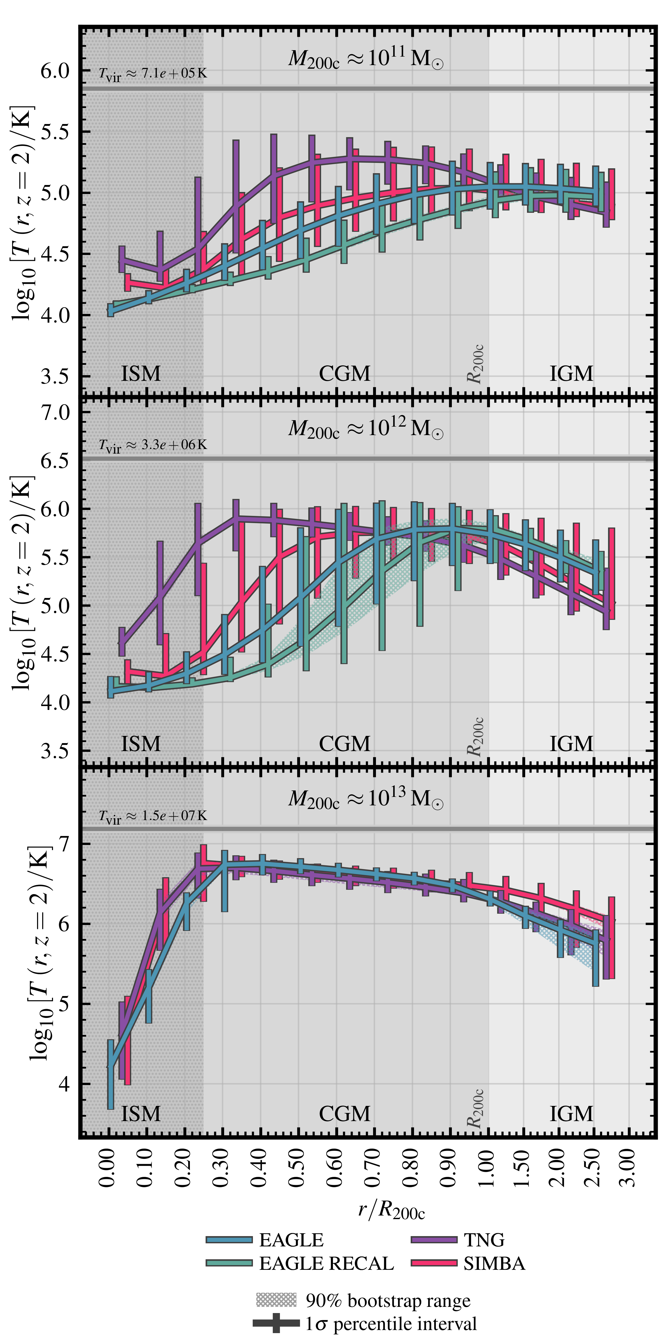
Figure 13: Radial temperature profiles of galaxies at $z=$ in EAGLE (blue), EAGLE-RECAL (teal), TNG (purple) and SIMBA (pink). Each row represents a different bin in halo mass, increasing top to bottom. Error-bars correspond to the $16^{\rm th}-84^{\rm th}$ percentile range in inflow rates at a given mass, and hatched regions correspond to the bootstrap-generated $90\%$ confidence interval on the medians at a given mass. Temperature predictions diverge between the simulations at this redshift in the two lower mass bins, particularly in the inner CGM.

Appendix D Halo baryon fractions at redshift 2

In this section, we add to the $z\approx 0$ results shown in §3 to compare the total baryon content of haloes at as a function of halo mass, and how this baryon content is distributed between stars, cool gas, and hot gas in each of the simulations. As in the main body of this paper, in each simulation, we define “cool gas” as the gas that is either considered star-forming, or below $5\times 10^{4}{\rm K}$, and “hot gas” as the remaining gas within $R_{\rm 200c}$ that does not meet this criteria.

At this redshift, the baryon content of haloes is universally higher in the simulations – for $M_{\rm 200c}\gtrsim 10^{11.5}{\rm M}_{\odot}$, all simulations predict a baryon fraction above $50\%$ of the cosmic mean. Similar to $z\approx 0$, the baryon content of EAGLEgalaxies at low halo mass – $M_{\rm 200c}\lesssim 10^{12}{\rm M}_{\odot}$ – is lower than the predictions from SIMBA and TNG, indicating that the ejective and preventative influence of stellar feedback is already at play by $z\approx 2$. The transition masses ${\mathcal{M}}^{{\rm T}_{1}}$ and ${\mathcal{M}}^{{\rm T}_{2}}$ are similar to those reported at $z\approx 0$, with the exception of SIMBA, where the ${\mathcal{M}}^{{\rm T}_{1}}$ mass at $z\approx 2$ increases to $\approx 10^{12}{\rm M}_{\odot}$ (as opposed to $\approx 10^{11.3}{\rm M}_{\odot}$ at $z\approx 0$, with ${\mathcal{M}}^{{\rm T}_{2}}$ remaining at $\approx 10^{12.8}{\rm M}_{\odot}$). For SIMBA, this indicates that AGN feedback becomes more efficient at lower masses towards $z\approx 0$.

References

- Ade et al. (2019) Ade P., et al., 2019, J. Cosmology Astropart. Phys., 2019, 056
- Akino et al. (2022) Akino D., et al., 2022, PASJ, 74, 175
- Anglés-Alcázar et al. (2017a) Anglés-Alcázar D., Davé R., Faucher-Giguère C.-A., Özel F., Hopkins P. F., 2017a, MNRAS, 464, 2840
- Anglés-Alcázar et al. (2017b) Anglés-Alcázar D., Faucher-Giguère C.-A., Kereš D., Hopkins P. F., Quataert E., Murray N., 2017b, MNRAS, 470, 4698
- Appleby et al. (2021) Appleby S., Davé R., Sorini D., Storey-Fisher K., Smith B., 2021, MNRAS, 507, 2383
- Appleby et al. (2023) Appleby S., Davé R., Sorini D., Lovell C. C., Lo K., 2023, MNRAS, 525, 1167
- Augustin et al. (2019) Augustin R., et al., 2019, MNRAS, 489, 2417
- Ayromlou et al. (2023) Ayromlou M., Nelson D., Pillepich A., 2023, MNRAS, 524, 5391
- Behroozi et al. (2019) Behroozi P., Wechsler R. H., Hearin A. P., Conroy C., 2019, MNRAS, 488, 3143
- Bondi (1952) Bondi H., 1952, MNRAS, 112, 195
- Bouché et al. (2016) Bouché N., et al., 2016, ApJ, 820, 121
- Bregman et al. (2022) Bregman J. N., Hodges-Kluck E., Qu Z., Pratt C., Li J.-T., Yun Y., 2022, ApJ, 928, 14
- Bryan & Norman (1998) Bryan G. L., Norman M. L., 1998, ApJ, 495, 80
- Chabrier (2003) Chabrier G., 2003, PASP, 115, 763
- Chadayammuri et al. (2022) Chadayammuri U., Bogdán Á., Oppenheimer B. D., Kraft R. P., Forman W. R., Jones C., 2022, ApJ, 936, L15
- Chisholm et al. (2016) Chisholm J., Tremonti Christy A., Leitherer C., Chen Y., 2016, MNRAS, 463, 541
- Christensen et al. (2016) Christensen C. R., Davé R., Governato F., Pontzen A., Brooks A., Munshi F., Quinn T., Wadsley J., 2016, ApJ, 824, 57
- Correa et al. (2018a) Correa C. A., Schaye J., Wyithe J. S. B., Duffy A. R., Theuns T., Crain R. A., Bower R. G., 2018a, MNRAS, 473, 538
- Correa et al. (2018b) Correa C. A., Schaye J., van de Voort F., Duffy A. R., Wyithe J. S. B., 2018b, MNRAS, 478, 255
- Crain & van de Voort (2023) Crain R. A., van de Voort F., 2023, ARA&A, 61, 473
- Crain et al. (2015) Crain R. A., et al., 2015, MNRAS, 450, 1937
- Dalla Vecchia & Schaye (2012) Dalla Vecchia C., Schaye J., 2012, MNRAS, 426, 140
- Davé et al. (2016) Davé R., Thompson R., Hopkins P. F., 2016, MNRAS, 462, 3265
- Davé et al. (2019) Davé R., Anglés-Alcázar D., Narayanan D., Li Q., Rafieferantsoa M. H., Appleby S., 2019, MNRAS, 486, 2827
- Davé et al. (2020) Davé R., Crain R. A., Stevens A. R. H., Narayanan D., Saintonge A., Catinella B., Cortese L., 2020, MNRAS, 497, 146
- Davies et al. (2019a) Davies L. J. M., et al., 2019a, MNRAS, 483, 1881
- Davies et al. (2019b) Davies L. J. M., et al., 2019b, MNRAS, 483, 5444
- DeFelippis et al. (2021) DeFelippis D., Bouché N. F., Genel S., Bryan G. L., Nelson D., Marinacci F., Hernquist L., 2021, ApJ, 923, 56
- Delgado et al. (2023) Delgado A. M., et al., 2023, arXiv e-prints, p. arXiv:2301.02231
- Dev et al. (2023) Dev A., et al., 2023, MNRAS, 523, 2693
- Dolag et al. (2009) Dolag K., Borgani S., Murante G., Springel V., 2009, MNRAS, 399, 497
- Dubois et al. (2014) Dubois Y., et al., 2014, MNRAS, 444, 1453
- Fabian (2012) Fabian A. C., 2012, ARA&A, 50, 455
- Faucher-Giguère et al. (2009) Faucher-Giguère C.-A., Lidz A., Zaldarriaga M., Hernquist L., 2009, ApJ, 703, 1416
- Ferrarese & Ford (2005) Ferrarese L., Ford H., 2005, Space Sci. Rev., 116, 523
- Feruglio et al. (2010) Feruglio C., Maiolino R., Piconcelli E., Menci N., Aussel H., Lamastra A., Fiore F., 2010, A&A, 518, L155
- Fielding et al. (2020) Fielding D. B., et al., 2020, ApJ, 903, 32
- Ford et al. (2014) Ford A. B., Davé R., Oppenheimer B. D., Katz N., Kollmeier J. A., Thompson R., Weinberg D. H., 2014, MNRAS, 444, 1260
- Furlong et al. (2015) Furlong M., et al., 2015, MNRAS, 450, 4486
- Gebhardt et al. (2023) Gebhardt M., et al., 2023, arXiv e-prints, p. arXiv:2307.11832
- Genel et al. (2013) Genel S., Vogelsberger M., Nelson D., Sijacki D., Springel V., Hernquist L., 2013, MNRAS, 435, 1426
- Gonzalez et al. (2013) Gonzalez A. H., Sivanandam S., Zabludoff A. I., Zaritsky D., 2013, ApJ, 778, 14
- Haardt & Madau (2001) Haardt F., Madau P., 2001, in Neumann D. M., Tran J. T. V., eds, Clusters of Galaxies and the High Redshift Universe Observed in X-rays. p. 64
- Harris et al. (2020) Harris C. R., et al., 2020, Nature, 585, 357
- Heckman & Best (2014) Heckman T. M., Best P. N., 2014, ARA&A, 52, 589
- Heckman et al. (2000) Heckman T. M., Lehnert M. D., Strickland D. K., Armus L., 2000, ApJS, 129, 493
- Heckman et al. (2015) Heckman T. M., Alexandroff R. M., Borthakur S., Overzier R., Leitherer C., 2015, ApJ, 809, 147
- Hoekstra et al. (2015) Hoekstra H., Herbonnet R., Muzzin A., Babul A., Mahdavi A., Viola M., Cacciato M., 2015, MNRAS, 449, 685
- Hopkins (2015) Hopkins P. F., 2015, MNRAS, 450, 53
- Hopkins (2017) Hopkins P. F., 2017, arXiv e-prints, p. arXiv:1712.01294
- Hopkins & Quataert (2011) Hopkins P. F., Quataert E., 2011, MNRAS, 415, 1027
- Hopkins et al. (2014) Hopkins P. F., Kereš D., Oñorbe J., Faucher-Giguère C.-A., Quataert E., Murray N., Bullock J. S., 2014, MNRAS, 445, 581
- Hopkins et al. (2018) Hopkins P. F., et al., 2018, MNRAS, 480, 800
- Hotan et al. (2021) Hotan A. W., et al., 2021, Publ. Astron. Soc. Australia, 38, e009
- Hunter (2007) Hunter J. D., 2007, Computing in Science and Engineering, 9, 90
- Jenkins (2013) Jenkins A., 2013, MNRAS, 434, 2094
- Jones et al. (2018) Jones M. G., Haynes M. P., Giovanelli R., Moorman C., 2018, MNRAS, 477, 2
- Katz et al. (1992) Katz N., Hernquist L., Weinberg D. H., 1992, ApJ, 399, L109
- Kennicutt (1983) Kennicutt R. C., 1983, The Astrophysical Journal, 272, 54
- Kennicutt (1998) Kennicutt R. C., 1998, ApJ, 498, 541
- Kennicutt & Evans (2012) Kennicutt R. C., Evans N. J., 2012, ARA&A, 50, 531
- Kereš et al. (2005) Kereš D., Katz N., Weinberg D. H., Davé R., 2005, MNRAS, 363, 2
- King & Pounds (2015) King A., Pounds K., 2015, ARA&A, 53, 115
- Kormendy & Ho (2013) Kormendy J., Ho L. C., 2013, ARA&A, 51, 511
- Krumholz & Gnedin (2011) Krumholz M. R., Gnedin N. Y., 2011, ApJ, 729, 36
- Kugel et al. (2023) Kugel R., et al., 2023, arXiv e-prints, p. arXiv:2306.05492
- Laganá et al. (2013) Laganá T. F., Martinet N., Durret F., Lima Neto G. B., Maughan B., Zhang Y. Y., 2013, A&A, 555, A66
- Lagos et al. (2015) Lagos C. d. P., et al., 2015, MNRAS, 452, 3815
- Lehner et al. (2013) Lehner N., et al., 2013, ApJ, 770, 138
- Leroy et al. (2015) Leroy A. K., et al., 2015, ApJ, 814, 83
- Lin et al. (2012) Lin Y.-T., Stanford S. A., Eisenhardt P. R. M., Vikhlinin A., Maughan B. J., Kravtsov A., 2012, ApJ, 745, L3
- Lokhorst et al. (2019) Lokhorst D., Abraham R., van Dokkum P., Wijers N., Schaye J., 2019, ApJ, 877, 4
- Lovisari et al. (2015) Lovisari L., Reiprich T. H., Schellenberger G., 2015, A&A, 573, A118
- Lovisari et al. (2020) Lovisari L., et al., 2020, ApJ, 892, 102
- Macquart et al. (2020) Macquart J. P., et al., 2020, Nature, 581, 391
- Madau & Dickinson (2014) Madau P., Dickinson M., 2014, ARA&A, 52, 415
- Maddox et al. (2021) Maddox N., et al., 2021, A&A, 646, A35
- Martin (2005) Martin C. L., 2005, ApJ, 621, 227
- Martin et al. (2012) Martin C. L., Shapley A. E., Coil A. L., Kornei K. A., Bundy K., Weiner B. J., Noeske K. G., Schiminovich D., 2012, ApJ, 760, 127
- Martin et al. (2019) Martin C. L., Ho S. H., Kacprzak G. G., Churchill C. W., 2019, ApJ, 878, 84
- Maughan et al. (2008) Maughan B. J., Jones C., Forman W., Van Speybroeck L., 2008, ApJS, 174, 117
- McCourt et al. (2018) McCourt M., Oh S. P., O’Leary R., Madigan A.-M., 2018, MNRAS, 473, 5407
- McKee & Ostriker (2007) McKee C. F., Ostriker E. C., 2007, ARA&A, 45, 565
- Mitchell et al. (2018) Mitchell P. D., et al., 2018, MNRAS, 474, 492
- Mitchell et al. (2020) Mitchell P. D., Schaye J., Bower R. G., Crain R. A., 2020, MNRAS, 494, 3971
- Moster et al. (2018) Moster B. P., Naab T., White S. D. M., 2018, MNRAS, 477, 1822
- Mulroy et al. (2019) Mulroy S. L., et al., 2019, MNRAS, 484, 60
- Muratov et al. (2015) Muratov A. L., Kereš D., Faucher-Giguère C.-A., Hopkins P. F., Quataert E., Murray N., 2015, MNRAS, 454, 2691
- Murray et al. (2005) Murray N., Quataert E., Thompson T. A., 2005, ApJ, 618, 569
- Murray et al. (2013) Murray S. G., Power C., Robotham A. S. G., 2013, Astronomy and Computing, 3, 23
- NAS (2021) NAS 2021, Pathways to Discovery in Astronomy and Astrophysics for the 2020s, doi:10.17226/26141.
- Naab & Ostriker (2017) Naab T., Ostriker J. P., 2017, ARA&A, 55, 59
- Neistein et al. (2012) Neistein E., Khochfar S., Dalla Vecchia C., Schaye J., 2012, MNRAS, 421, 3579
- Nelson et al. (2019) Nelson D., et al., 2019, MNRAS, 490, 3234
- Newman et al. (2012) Newman S. F., et al., 2012, ApJ, 761, 43
- Ni et al. (2023) Ni Y., et al., 2023, arXiv e-prints, p. arXiv:2304.02096
- Oppenheimer & Davé (2006) Oppenheimer B. D., Davé R., 2006, MNRAS, 373, 1265
- Oppenheimer et al. (2018) Oppenheimer B. D., Schaye J., Crain R. A., Werk J. K., Richings A. J., 2018, MNRAS, 481, 835
- Oppenheimer et al. (2020) Oppenheimer B. D., et al., 2020, MNRAS, 491, 2939
- Pakmor et al. (2011) Pakmor R., Bauer A., Springel V., 2011, MNRAS, 418, 1392
- Pandya et al. (2020) Pandya V., et al., 2020, ApJ, 905, 4
- Pandya et al. (2021) Pandya V., et al., 2021, MNRAS, 508, 2979
- Pearson et al. (2017) Pearson R. J., et al., 2017, MNRAS, 469, 3489
- Péroux et al. (2020) Péroux C., Nelson D., van de Voort F., Pillepich A., Marinacci F., Vogelsberger M., Hernquist L., 2020, MNRAS, 499, 2462
- Pillepich et al. (2018) Pillepich A., et al., 2018, MNRAS, 473, 4077
- Planck Collaboration et al. (2014) Planck Collaboration et al., 2014, A&A, 571, A16
- Planck Collaboration et al. (2016) Planck Collaboration et al., 2016, A&A, 594, A13
- Pratt et al. (2010) Pratt G. W., et al., 2010, A&A, 511, A85
- Predehl et al. (2021) Predehl P., et al., 2021, A&A, 647, A1
- Prochaska et al. (2017) Prochaska J. X., et al., 2017, ApJ, 837, 169
- Rasmussen & Ponman (2009) Rasmussen J., Ponman T. J., 2009, MNRAS, 399, 239
- Rubin (2017) Rubin K. H. R., 2017, in Fox A., Davé R., eds, Astrophysics and Space Science Library, Vol. 430, Gas Accretion onto Galaxies , Astrophysics and Space Science Library, Volume 430. ISBN 978-3-319-52511-2. Springer International Publishing AG, 2017, p. 95. p. 95, doi:10.1007/978-3-319-52512-9_5
- Rubin et al. (2012) Rubin K. H. R., Prochaska J. X., Koo D. C., Phillips A. C., 2012, ApJ, 747, L26
- Rubin et al. (2014) Rubin K. H. R., Prochaska J. X., Koo D. C., Phillips A. C., Martin C. L., Winstrom L. O., 2014, ApJ, 794, 156
- Rupke et al. (2019) Rupke D. S. N., et al., 2019, Nature, 574, 643
- Saintonge et al. (2017) Saintonge A., et al., 2017, ApJS, 233, 22
- Sánchez Almeida et al. (2014) Sánchez Almeida J., Elmegreen B. G., Muñoz-Tuñón C., Elmegreen D. M., 2014, A&ARv, 22, 71
- Sanderson et al. (2013) Sanderson A. J. R., O’Sullivan E., Ponman T. J., Gonzalez A. H., Sivanandam S., Zabludoff A. I., Zaritsky D., 2013, MNRAS, 429, 3288
- Schaller et al. (2015) Schaller M., Dalla Vecchia C., Schaye J., Bower R. G., Theuns T., Crain R. A., Furlong M., McCarthy I. G., 2015, MNRAS, 454, 2277
- Schaye & Dalla Vecchia (2008) Schaye J., Dalla Vecchia C., 2008, MNRAS, 383, 1210
- Schaye et al. (2007) Schaye J., Carswell R. F., Kim T.-S., 2007, MNRAS, 379, 1169
- Schaye et al. (2010) Schaye J., et al., 2010, MNRAS, 402, 1536
- Schaye et al. (2015) Schaye J., et al., 2015, MNRAS, 446, 521
- Schaye et al. (2023) Schaye J., et al., 2023, MNRAS,
- Schroetter et al. (2016) Schroetter I., et al., 2016, ApJ, 833, 39
- Smith et al. (2008) Smith B., Sigurdsson S., Abel T., 2008, MNRAS, 385, 1443
- Smith et al. (2017) Smith B. D., et al., 2017, MNRAS, 466, 2217
- Somerville & Davé (2015) Somerville R. S., Davé R., 2015, Annual Review of Astronomy and Astrophysics, 53, 51
- Sorini et al. (2022) Sorini D., Davé R., Cui W., Appleby S., 2022, MNRAS, 516, 883
- Springel (2005) Springel V., 2005, MNRAS, 364, 1105
- Springel (2010) Springel V., 2010, MNRAS, 401, 791
- Springel & Hernquist (2003) Springel V., Hernquist L., 2003, MNRAS, 339, 289
- Springel et al. (2001) Springel V., Yoshida N., White S. D. M., 2001, New Astron., 6, 79
- Springel et al. (2005) Springel V., Di Matteo T., Hernquist L., 2005, ApJ, 620, L79
- Springel et al. (2018) Springel V., et al., 2018, MNRAS, 475, 676
- Stinson et al. (2006) Stinson G., Seth A., Katz N., Wadsley J., Governato F., Quinn T., 2006, MNRAS, 373, 1074
- Stone et al. (2016) Stone M., Veilleux S., Meléndez M., Sturm E., Graciá-Carpio J., González-Alfonso E., 2016, ApJ, 826, 111
- Sun et al. (2009) Sun M., Voit G. M., Donahue M., Jones C., Forman W., Vikhlinin A., 2009, ApJ, 693, 1142
- Thomas et al. (2019) Thomas N., Davé R., Anglés-Alcázar D., Jarvis M., 2019, MNRAS, 487, 5764
- Thorne et al. (2021) Thorne J. E., et al., 2021, MNRAS, 505, 540
- Tillman et al. (2023a) Tillman M. T., et al., 2023a, AJ, 166, 228
- Tillman et al. (2023b) Tillman M. T., Burkhart B., Tonnesen S., Bird S., Bryan G. L., Anglés-Alcázar D., Davé R., Genel S., 2023b, ApJ, 945, L17
- Tollet et al. (2019) Tollet É., Cattaneo A., Macciò A. V., Dutton A. A., Kang X., 2019, MNRAS, 485, 2511
- Tumlinson et al. (2013) Tumlinson J., et al., 2013, ApJ, 777, 59
- Tumlinson et al. (2017) Tumlinson J., Peeples M. S., Werk J. K., 2017, ARA&A, 55, 389
- Veilleux et al. (2005) Veilleux S., Cecil G., Bland-Hawthorn J., 2005, ARA&A, 43, 769
- Veilleux et al. (2020) Veilleux S., Maiolino R., Bolatto A. D., Aalto S., 2020, A&ARv, 28, 2
- Vikhlinin et al. (2006) Vikhlinin A., Kravtsov A., Forman W., Jones C., Markevitch M., Murray S. S., Van Speybroeck L., 2006, ApJ, 640, 691
- Villaescusa-Navarro et al. (2021) Villaescusa-Navarro F., et al., 2021, ApJ, 915, 71
- Virtanen et al. (2020) Virtanen P., et al., 2020, Nature Methods, 17, 261
- Vogelsberger et al. (2014) Vogelsberger M., et al., 2014, MNRAS, 444, 1518
- Vogelsberger et al. (2020) Vogelsberger M., Marinacci F., Torrey P., Puchwein E., 2020, Nature Reviews Physics, 2, 42
- Wadsley et al. (2004) Wadsley J. W., Stadel J., Quinn T., 2004, New Astron., 9, 137
- Wang et al. (2015) Wang L., Dutton A. A., Stinson G. S., Macciò A. V., Penzo C., Kang X., Keller B. W., Wadsley J., 2015, MNRAS, 454, 83
- Weinberger et al. (2017) Weinberger R., et al., 2017, MNRAS, 465, 3291
- Werk et al. (2014) Werk J. K., et al., 2014, ApJ, 792, 8
- Wiersma et al. (2009) Wiersma R. P. C., Schaye J., Theuns T., Dalla Vecchia C., Tornatore L., 2009, MNRAS, 399, 574
- Wright et al. (2020) Wright R. J., Lagos C. d. P., Power C., Mitchell P. D., 2020, MNRAS, 498, 1668
- Wright et al. (2021) Wright R. J., Lagos C. d. P., Power C., Correa C. A., 2021, MNRAS, 504, 5702
- Yang et al. (2022) Yang T., Cai Y.-C., Cui W., Davé R., Peacock J. A., Sorini D., 2022, MNRAS, 516, 4084
- Zabl et al. (2019) Zabl J., et al., 2019, MNRAS, 485, 1961
- Zahedy et al. (2019) Zahedy F. S., Chen H.-W., Johnson S. D., Pierce R. M., Rauch M., Huang Y.-H., Weiner B. J., Gauthier J.-R., 2019, MNRAS, 484, 2257
- van Rossum & Drake Jr (1995) van Rossum G., Drake Jr F. L., 1995, Python reference manual. Centrum voor Wiskunde en Informatica Amsterdam
- van de Voort (2017) van de Voort F., 2017, in Fox A., Davé R., eds, Astrophysics and Space Science Library Vol. 430, Gas Accretion onto Galaxies. p. 301, doi:10.1007/978-3-319-52512-9_13