Abstract

Bayesian optimization is a methodology to optimize black-box functions. Traditionally, it focuses on the setting where you can arbitrarily query the search space. However, many real-life problems do not offer this flexibility; in particular, the search space of the next query may depend on previous ones. Example challenges arise in the physical sciences in the form of local movement constraints, required monotonicity in certain variables, and transitions influencing the accuracy of measurements. Altogether, such transition constraints necessitate a form of planning. This work extends Bayesian optimization via the framework of Markov Decision Processes, iteratively solving a tractable linearization of our objective using reinforcement learning to obtain a policy that plans ahead over long horizons. The resulting policy is potentially history-dependent and non-Markovian. We showcase applications in chemical reactor optimization, informative path planning, machine calibration, and other synthetic examples.

1 Introduction

Many areas in the natural sciences and engineering deal with optimizing expensive black-box functions. Bayesian optimization (BayesOpt) (Shahriari et al., 2016; Jones et al., 1998), a method to optimize these problems using a probabilistic surrogate, has successfully addressed these problems. It has been applied to a myriad of examples, e.g. tuning the hyper-parameters of expensive-to-train models (Hutter et al., 2019), robotics (Marco et al., 2017), battery design (Folch et al., 2023a), and drug discovery (Brennan et al., 2022) among many others. However, state-of-the-art algorithms are often ill-suited for physical sciences interacting with potentially dynamic systems. In such circumstances, real-life constraints limit our future decisions depending on the prior state of our interaction with the system. This work focuses chiefly on transition constraints influencing future choices depending on the current state of the experiment. In other words, reaching certain parts of the decision space (search space) requires long-term planning in our optimization campaign. This effectively means we address a general sequential-decision problem akin to those studied in reinforcement learning (RL) or optimal control. Unique to our setting, we assume the transition constraints are known a priori. We focus on problems where “large” (in application-specific metrics) changes between sequential decision steps are infeasible. In such a setting, we can try to minimise the decision changes or constrain these to reasonable values.

Applications with transition constraints include chemical reaction optimization (Vellanki et al., 2017; Folch et al., 2022), environmental monitoring (Bogunovic et al., 2016; Mutny et al., 2023), lake surveillance with drones (Hitz et al., 2014; Gotovos et al., 2013; Samaniego et al., 2021), energy systems (Ramesh et al., 2022), vapor compression systems (Paulson et al., 2023), electron-laser tuning Kirschner et al. (2022), seabed identification (Sullivan et al., 2023), and source seeking (Mishra et al., 2023). For example, Figure 1 depicts an application in environmental monitoring where autonomous sensing vehicles must avoid obstacles (in a similar fashion to  Hitz et al. (2014)). Here, we focus on transient flow reactors Mozharov et al. (2011); Schrecker et al. (2023) as a motivating application. Such reactors allow efficient data collection by obtaining semi-continuous time-series data rather than waiting for the system to reach a steady state. However, as we can change inputs of the reactor only continuously, allowing arbitrary changes (as in conventional BayesOpt) is a non-physical simplification of the system. Frequently, we also face additional constraints, such as monotonicity in the paths created.

1.1 Problem Statement

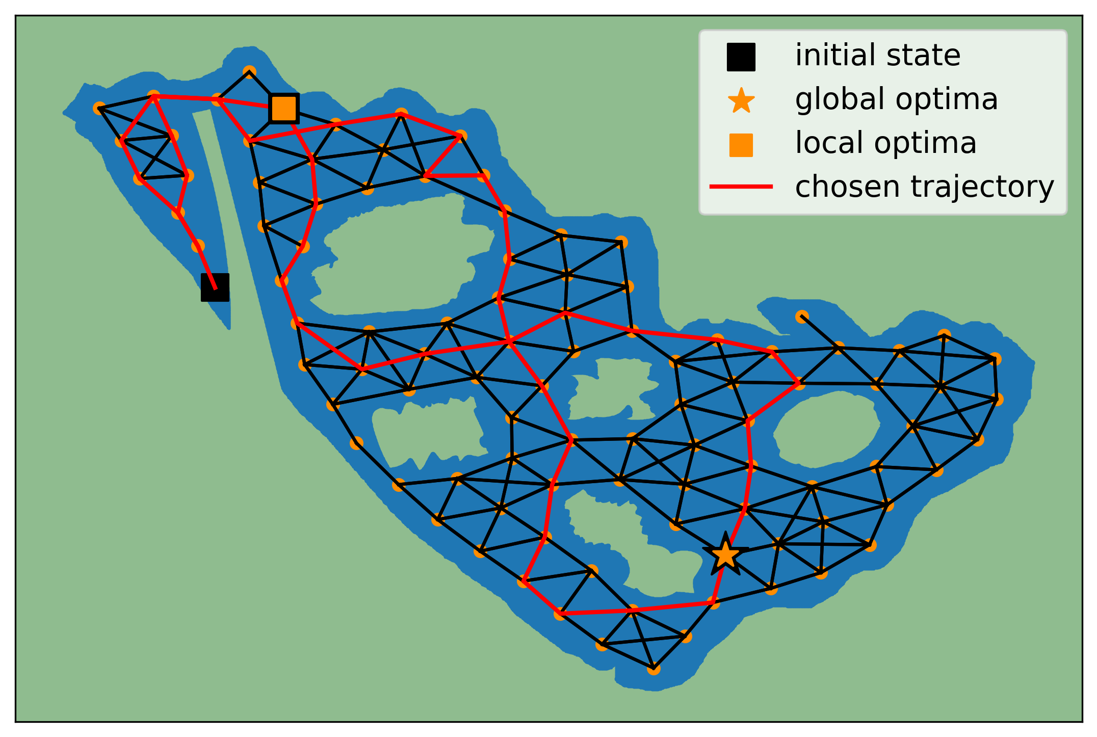
Figure 1: Map depicting lake Ypacarai with the discretized state space and allowed transitions as the edges in black. The constraints stipulate movement only over the edges. Our task is to identify the maximal pollution source (orange star). The black square denotes the initial and endpoints, and the orange square is a local optimum. The red line is an initial trajectory chosen by our algorithm.

Mathematically, we want to identify the best configuration of a physical system governed by a black box function $f$,

$$x^{\star}=\arg\max_{x\in\mathcal{X}}f(x)$$ (1)

where $f$ is modeled as a Gaussian process with a known kernel $k$, and $\mathcal{X}$ is our possible system configuration, also called the search space. In addition, we assume known dynamics that dictate how we can choose $x\in\mathcal{X}$. The function $f$ is unknown, and we improve our estimate of it.

1.2 Related Works & Contributions

BayesOpt chooses experiments that maximize a myopic utility. Typically, one assumes one can sample any point in the search space $\mathcal{X}$. However, when local constraints are involved, we must traverse the search space to reach the desired configuration first. Solving these problems requires planning for long horizons, sometimes called multi-step, look-ahead optimization or optimization over sequences.

Multi-step utilities. Look-ahead BayesOpt allows for planning by considering utilities reflecting joint decisions (Ginsbourger & Le Riche, 2010; Lam et al., 2016; Jiang et al., 2020; Lee et al., 2021; Paulson et al., 2022; Cheon et al., 2022). This, however, comes at a high computational cost of simulating inference, and the complexity can grow exponentially with the number of look-ahead steps. The short horizons considered are insufficient for applications with reasonably sized decision sets $\mathcal{X}$ or tight movement constraints. To address these inefficiencies, heuristics resort to truncation strategies (Samaniego et al., 2021; Paulson et al., 2023), which only work for specific transition constraints.

Optimizing over sequences. Instead of planning ahead, one could instead ignore the adaptive feedback and optimize a path (Folch et al., 2022; Ramesh et al., 2022; Yang et al., 2023). These works focus on the case where there is a cost of changing between subsequent queries and try to solve the optimization while minimizing movement costs. However, they do not adhere to strict constraints as we do.

Best-arm identification. While BayesOpt is usually stated in the context of finding the optimal input of black-box function, most algorithms focus on regret minimization. This work focuses on maximizer identification directly, i.e., to identify the maximum after a certain number of iterations with the highest confidence. This branch of BayesOpt is mostly addressed in the bandit literature Audibert & Bubeck (2010). Our proposed objective builds upon prior works of Soare et al. (2014); Yu et al. (2006), and follows the approach of Fiez et al. (2019) except that we encounter an added difficulty with the transition constraints in our setting. Concurrent work of Che et al. (2023) tackles a constrained variant of a similar problem using model predictive control, sharing many similarities in the problem setting and solution with our work while using a different objective.

Contributions. Our new BayesOpt approach tractably plans over the whole experimentation horizon and considers Markov transition constraints, building on active exploration (Mutny et al., 2023) and best-arm identification (Fiez et al., 2019). Our key contributions include:

• We consider a local approximation of multi-step prediction BayesOpt, and we greedily optimize it. This results in a tractable, not exponentially scaling (in $H$) optimization problem that is, in many cases, convex.

• To do so, we introduce a new objective in connection with the experiment design in Markov Chains for maximizer identification.

• We provide practical solutions to the optimisation problem for both discrete and continuous Markov Decision Processes, and establish an informal relation to model predictive control. Our resulting optimal policies are efficient and history-dependent.

• We empirically demonstrate the practicality of the approach on various problems with transition constraints.

2 Background: Experiment Design

We now review relevant background from experimental design, BayesOpt, and RL that we build on.

2.1 Optimization of Gaussian Processes

To model the unknown function $f$ as in Eq. (1), we use Gaussian processes (GPs). GPs are probabilistic models capturing nonlinear functional relationships and offering well-calibrated uncertainty estimates. All finite marginals, e.g., values $\{f(x_{j})\}_{j}$, are normally distributed. For probabilistic modeling, we adopt a Bayesian approach, and assume $f$ is a sample from a GP prior with a known kernel, $k$, and zero mean function, $f\sim\operatorname{GP}(0,k)$. We assume that we can obtain noisy observations of $f$ for a given $x\in\mathcal{X}$,

$$y=f(x)+\epsilon(x),$$

where $\epsilon$ has a known Gaussian likelihood, which is possibly heteroscedastic (Kirschner & Krause, 2018), and depends on both $x\in\mathcal{X}$ (and potentially actions $\mathcal{A}$, see Sec. 2.3). Under these assumptions, the posterior of $f$ given observed data will also be a GP, and the form of the posterior can be analytically calculated (Rasmussen & Williams, 2005).

BayesOpt seeks to optimize expensive black-box functions through sequential querying of points, chosen by greedily maximizing an acquisition function, $\alpha$:

$$x_{t+1}=\operatorname*{arg\,max}_{x\in\mathcal{X}}\alpha(x|\mathbf{X}_{t}),$$ (2)

where $\mathbf{X}_{t}$ is the available data at iteration $t$. The function arises as a greedy one-step approximation of an overall utility function for the optimization task. In the following section, we will show what overall utility is used in our problem, and how we can implement the policy variant where optimization is done not on queries $x\in\mathcal{X}$, but instead policies $\pi$ that act on $\mathcal{X}$.

2.2 Best-Arm Identification: Experiment Design Goal

BayesOpt is naturally myopic in its definition as a greedy one-step update (see (2)). Non-myopic behaviour can be induced by selecting $\alpha$ in a meaningful way. The probabilistic framework allows for long-term planning in BayesOpt, namely anticipating the outcomes of planned observations and optimizing over sequences of decisions (Osborne et al., 2009). This is, however, highly computationally burdensome, as it requires simulations from the posterior or heuristic approximations (Jiang et al., 2020). The uncertainty in possible experiment observations must be averaged, leading to large integrals and the need to use Monte Carlo estimates. To build an objective that can be tractable when used for planning, we instead focus on a continuous reformulation of the objective over visited states, which allows for efficient planning, as we will demonstrate. Moreover, our objective is motivated by optimal hypothesis testing.

Best-Arm Identification. We focus on identifying $x^{\star}$, the maximizer of $f$. This can be formulated as a multiple hypothesis testing problem, where we need to determine which of the elements in $\mathcal{X}$ is the maximizer. To identify the maximizer, we need to understand the differences between individual arms $f(x_{i})-f(x_{j})$, namely their signs, where $x_{i},x_{j}\in\mathcal{X}$.

Therefore, if we assume that we have access to a set of potential maximizers, $\mathcal{Z}$, containing the true best-arm, and letting $\mathbf{X}_{t}$ be the set of evaluations that we have selected previously, we will choose a new set of experiments $\mathbf{X}_{\text{new}}$ such that we try to minimize the largest variance:

$$\min_{\mathbf{X}_{\text{new}}}\max_{z^{\prime}\in\mathcal{Z}}\text{Var}[f(x^{*})-f(z^{\prime})|\mathbf{X}_{t}\cup\mathbf{X}_{\text{new}}]$$ (3)

i.e., we minimize the worst-case (maximum) uncertainty gap among points in $\mathcal{Z}$. However, the distribution of $f(x^{\star})$ is highly complicated and non-trivial (Hennig & Schuler, 2012), making the above objective intractable. Instead, we propose working with the tractable upper bound on Eq. (3):

$$U(\mathbf{X}_{\text{new}})=\max_{z^{\prime},z\in\mathcal{Z}}\text{Var}[f(z)-f(z^{\prime})|\mathbf{X}_{t}\cup\mathbf{X}_{\text{new}}].$$ (4)

Such objectives can be solved greedily in a similar way as acquisition functions in Eq. (2) by minimizing $U$ over $\mathbf{X}_{\text{new}}$.

Approximation of Gaussian Processes. The objective involves constructing kernel matrices over the decision space $\mathcal{X}$. To mitigate the computational and exposition difficulty, we utilize finite-dimensional approximations of kernel $k$ based on Nyström features (Williams & Seeger, 2000). Other approximation techniques include Fourier features (Mutny & Krause, 2018; Rahimi & Recht, 2007). These formulations make the objectives considered in this work more tractable. The Nyström approximation gives us a method of creating $m$-dimensional feature vectors $\Phi(x)$ such that we can estimate the GP:

$$f(x)\approx\Phi(x)^{T}\theta\quad\text{and}\quad\theta\sim\mathcal{N}(0,\mathbf{I}_{m\times m})$$ (5)

See Appendix B for details. Importantly, with this approximation, the objective Eq. (4) can be written $U(\mathbf{X}_{\text{new}})=$

$$\max_{z,z^{\prime}\in\mathcal{Z}}||\Phi(z)-\Phi(z^{\prime})||^{2}_{\left(\sum_{x\in\mathbf{X}_{t}\cup\mathbf{X}_{\text{new}}}\frac{\Phi(x)\Phi(x)^{\top}}{\sigma^{2}}+\lambda\mathbf{I}\right)^{-1}},$$ (6)

which vastly simplifies the optimization process, as the matrix to be inverted is $m\times m$ instead of $n\times n$ (depending on the data) or, for generic planning, $|\mathcal{X}|\times|\mathcal{X}|$ (see Sec. 4).

2.3 Markov Decision Processes

To model the transition constraints, we use the versatile mathematical model of Markov Decision processes (MDPs). MDPs allow us to describe sequential decision-making problems in a formal manner. We assume we have an environment with state space $\mathcal{X}$ and action space $\mathcal{A}$, where we interact with an unknown function $f:\mathcal{X}\times\mathcal{A}\rightarrow\mathbb{R}$ by rolling out a policy for $H$ time-steps and obtain a trajectory:

$$\tau=(x_{0},a_{0},x_{1},a_{1},...,x_{H-1},a_{H-1}).$$

From the trajectory, we obtain a sequence of noisy observations $y(\tau):=\{y(x_{0},a_{0}),...,y(x_{H-1},a_{H-1})\}$ s.t. $y(x_{h})=f(x_{h},a_{h})+\epsilon(x_{h},a_{h})$, where $\epsilon(x_{h},a_{h})$ is zero-mean Gaussian with known variance which is potentially state and action dependent. The trajectory is generated using a known transition operator $P(x_{h+1}|x_{h},a_{h})$. A policy $\pi(a_{h}|x_{h})$ is a mapping that dictates the probability of action $a_{h}$ in state $h$. Hence, the state-to-state transitions are $P(x_{h+1},x_{h})=\sum_{a\in\mathcal{A}}\pi_{h}(a|x_{h})P(x_{h+1}|x_{h},a)$. In fact, an equivalent description of any Markov policy $\pi$ is its visitation of states and actions, which we denote $d\in\mathcal{D}$, where

$$\mathcal{D}:=\Big{\{}\forall h\in[H]~{}d_{h}~{}|~{}d_{h}(x,a)\geq 0,~{}\sum_{a,x}d_{h}(x,a)=1,$$

$$~{}\sum_{a}d_{h}(x^{\prime},a)=\sum_{x,a}d_{h-1}(x,a)p(x^{\prime}|x,a)\Big{\}}.$$

Any $d\in\mathcal{D}$ can be realized by a policy $\pi$ and vice-versa. Notice that for finite horizons, the policy is non-stationary (Puterman, 2014). We will use this polytope to reformulate our optimization problem over trajectories.

Notice that the execution of deterministic trajectories is only possible for deterministic transitions. Otherwise, the resulting trajectories are random. In our setup, we repeat interactions $T$ times (episodes) to obtain the final dataset of the form $\mathbf{X}_{T}=\{\tau_{i},y(\tau_{i})\}_{i=1}^{T}$.

2.4 Experiment Design in Markov Chains

The utility we will define is over trajectories in a Markov chain, and hence $\mathbf{X}_{t}$ forms a set of executed trajectories. Optimizing directly over trajectories would lead to an exponential blowup. Also, for random transitions, we cannot pick the trajectories defining the utility $U(\{\tau_{i},y(\tau_{i})\}_{i=1}^{T})$ exactly. Hence, we focus on expected utility over the randomness of the policy and the environment, namely:

$$U_{\mathbb{E}}(\{\pi\}_{t=1}^{T})=U(\mathbb{E}_{\tau_{1}\sim\pi_{1},\dots\tau_{t}\sim\pi_{t}}[\mathbf{X}_{t}]):=F(d_{\pi}).$$ (7)

The expectation looks at the expected trajectory data. Mutny et al. (2023) tractably solve such objectives that arise in experiments by performing planning in MDPs. Mutny et al. (2023) focus on learning linear operators of an unknown function, unlike identifying a maximum, as we do here. The key observation is that any policy $\pi$ induces a distribution over the space of trajectories, which in turn induces a probability distribution over the state-action visitations, $d_{\pi}$. Therefore we can reformulate the problem of finding the optimal policy, into finding the optimal distribution over state-action visitations as: $\min_{d_{\pi}\in\mathcal{D}}F(d_{\pi})$, we refer to this as the planning problem. The constraint $\mathcal{D}$ encodes the dynamics of the MDP (in our case, it encodes the transition constraints).

The framework requires the utility (a) can be expressed additively over the visited states, and (b) is convex with respect to the state-action visitation distribution for planning using convex optimization. Section 3.1 shows that the objective (6) (hence (4)) are compatible with this MDP framework. Section 4 details how to solve the planning problem to find an optimal state-action distribution.

3 Transition Constrained BayesOpt

This section introduces BayesOpt with MDPs for general discrete Markov chains and shows how it can be extended to continuous variables to allow for scalability in certain MDPs. We describe a formal way to include constraints into our framework and classify different forms of feedback.

Encoding Constraints. We assume that there exists a constraint in the decision-making process such that:

$$x_{h+1}\in\mathcal{C}(x_{h})$$ (8)

where $\mathcal{C}(x_{h})$ is a general constraint set, defining which inputs we are allowed to query at time-step $h+1$ given we previously queried $x_{h}$. We can encode this constraint into the MDP through the transition operator, by setting $P(x_{h+1}|x_{h},a)=0$ for any $x_{h+1}\notin\mathcal{C}(x_{h})$, $a\in\mathcal{A}$.

Feedback models. We consider two different types of feedback that coincide with the real-world execution of the experiment in chemical reactors:

• Episodic feedback is the setting where the optimization can be split into episodes. We obtain the whole set of noisy observations at the end of each episode.

• Instant feedback is the setting where we obtain a noisy observation immediately after querying the function. This is the standard in most BayesOpt literature.

In-between feedback such as asynchronous is also common.

3.1 Expected Utility for Maximizer Identification

Using the finite-dimensional distribution approximation of GPs in Sec. 2.2, Eq. (4) can be rewritten in terms of the state-action distribution induced by $\mathbf{X}_{\text{new}}$, $F(d_{\pi})=$

$$\max_{z,z^{\prime}\in\mathcal{Z}}||\Phi(z)-\Phi(z^{\prime})||^{2}_{\mathbf{V}(d_{\pi})^{-1}}$$ (9)

where $\mathbf{V}(d_{\pi})=\left(\sum_{x,a\in\mathcal{X}\times\mathcal{A}}\frac{d_{\pi}(x,a)\Phi(x,a)\Phi(x,a)^{\top}}{\sigma^{2}(x,a)}+\lambda\mathbf{I}\right)$. The variable $d_{\pi}(x,a)$ is a state-action visitation, $\Phi(x)$ are the Nyström features of the GP, and $\lambda$ is a regularization constant. We prove this in Lemma E.1 in Appendix E. This objective is equivalent to the linear bandits objective without transition constraints of Fiez et al. (2019), who provided non-asymptotic optimality guarantees for this objective. In particular, by rewriting it in this form, dependence and convexity with respect to the state-action density $d_{\pi}$ becomes clear, and we can make the immediate connection with the experiment design MDP framework introduced in Sec. 2.4.

Discrete vs Continuous MDPs. The above approximation is especially useful when working with continuous Markov chains. Until this point, our formulation focused on discrete $\mathcal{S}$ and $\mathcal{A}$. However, the framework is compatible with continuous state-action spaces as specified in (6). The probabilistic reformulation of the objective in Eq. (7) holds irrespective of properties of $\mathcal{X}$, whether a discrete or continuous subset of $\mathbb{R}^{d}$. The difference is that the visitations $d$ are no longer probability mass functions but have to be expressed as probability density functions $d_{c}(x)$. To recover probabilities in the definition of $\mathbf{V}$, we need to replace sums with integrals i.e.:

$$\sum_{x\in\mathcal{X}}d(x)\frac{\Phi(x)\Phi(x)^{\top}}{\sigma^{2}}\rightarrow\int_{x\in\mathcal{X}_{c}}d_{c}(x)\frac{\Phi(x)\Phi(x)^{\top}}{\sigma^{2}}.$$

where $\mathcal{X}_{c}$ designated that $\mathcal{X}$ is a interval subset of $\mathbb{R}^{d}$.

3.2 Set of potential maximizers $\mathcal{Z}$.

The definition of the objective requires the use of a set of maximizers. In the ideal case, we can say a particular input $x$, is not the optimum if there exists $x^{\prime}$ such that $f(x^{\prime})>f(x)$ with high confidence. We formalize this using the GP credible sets (Bayesian confidence sets) and define:

$$\mathcal{Z}=\left\{x\in\mathcal{X}:\text{UCB}(f(x))\geq\sup_{x^{\prime}\in\mathcal{X}}\text{LCB}(f(x^{\prime}))\right\}$$ (10)

where UCB and LCB correspond to the upper and lower confidence bounds of the GP surrogate, respectively.

Continuous MDPs.  Note that Eq. (9) requires taking a maximum over all input pairs in $\mathcal{Z}$, and, while this can be enumerated in the discrete case, it poses a non-trivial constrained optimization problem when $\mathcal{X}$ is continuous. As an alternative, we could approximate the set $\mathcal{Z}$ through Thompson Sampling (Kandasamy et al., 2018):

$$\mathcal{Z}_{cont}^{(TS)}=\left\{\operatorname*{arg\,max}_{x\in\mathcal{X}_{c}}f_{i}(x):f_{i}\sim\mathcal{GP}(\mu_{t},\sigma_{t})\right\}_{i=1}^{K}$$

where $K$ is a new hyper-parameter influencing the accuracy of the approximation of $\mathcal{Z}$. We found that the algorithm could be too exploratory in certain scenarios. Therefore, we also propose an alternative that encourages exploitation by guiding the maximization set using BayesOpt through the UCB acquisition function (Srinivas et al., 2009):

$$\mathcal{Z}_{cont}^{(UCB)}=\left\{\operatorname*{arg\,max}_{x\in\mathcal{X}_{c}}\mu_{t}(x)+\beta_{i}\sigma_{t}(x):\beta_{i}\in\mathcal{B}\right\}_{i=1}^{K}$$

where $\mathcal{B}=\texttt{linspace(0, 2.5, K)}$ which serves as scaling for the size of set $\mathcal{Z}_{cont}^{(UCB)}$. Both cases reduce optimization over $\mathcal{Z}$ to enumeration as with discrete cases.

Algorithm 1 Movement Constrained BayesOpt via MDPs

  Input: BayesOpt procedure for estimating sets of maximizers, initial point $x_{0}$, initial set of maximizers $\mathcal{Z}_{0}$

  Initialize the empirical state-action distribution $\hat{d}_{0}=0$

  for $t=0$ to $T-1$ do

     for $h=0$ to $H-1$ do

        $F_{t,h}(d_{\pi})\leftarrow F(d_{\pi}\oplus\hat{d}_{t,h}|\mathcal{Z}_{t,h},x_{t,h})$ // define the objective, see details in equation (9)

        $\pi_{t,h}=\operatorname*{arg\,min}_{\pi:d_{\pi}\in\mathcal{D}_{t,h}}F_{t,h}(d_{\pi})$ // solve MDP planning problem

        $x_{t,h+1}=\pi_{t,h}(x_{t,h})$ // deploy policy

        if feedback is immediate then

           $y_{t,h+1}=f(x_{t,h+1})+\epsilon_{t,h};\ \mathcal{GP}_{t,h},\ \mathcal{Z}_{t,h}\leftarrow\text{Update}(\mathbf{X}_{t,h},\mathbf{Y}_{t,h})$ // get observation, update set of maximizers

        $\hat{d}_{t,h+1}(x)\leftarrow\hat{d}_{t,h}\oplus\delta(x_{t,h+1},x)$ // update empirical state-action distribution

     if feedback is episodic then

        $\mathbf{Y}_{t,H}=f(\mathbf{X}_{t,H})+\vec{\epsilon}_{t,:};\ \mathcal{GP}_{t+1,:},\ \mathcal{Z}_{t+1,:}\leftarrow\text{Update}(\mathbf{X}_{t,H},\mathbf{Y}_{t,H})$ // get observations, update set of maximizers

  Return: Estimate of the maximum using the GP posterior’s mean $\hat{x}_{*}=\operatorname*{arg\,max}_{x\in\mathcal{X}}\mu_{T}(x)$

3.3 General algorithm

The general algorithm combines the ideas introduced so far. We present it in Algorithm 1 with all the available feedback options. Notice that apart from constructing the current utility, keeping track of the visited states and updating our GP model, an essential step is planning, where we need to find a policy that maximizes the utility. As this forms the core challenge of the algorithm, we devote Sec. 4 to it. Simply put, however, it solves a sequence of dynamic programming problems with the Frank-Wolfe algorithm.

4 Solving the planning problem

Let us understand the planning problem and how it can be solved in more detail. We are following the development in Hazan et al. (2019) and Mutny et al. (2023). Recall for a convex objective, $F$, we define the problem as:

$$\min_{d_{\pi}\in\mathcal{D}}F(d_{\pi})$$ (11)

Conveniently, the linear problem on the polytope $\mathcal{D}$ corresponds to an RL problem for which many efficient solvers exist. We use Frank-Wolfe (Jaggi, 2013) and decompose the problem into a series of linearizations (Hazan et al., 2019). By doing so, we can build a mixture policy consisting of optimal policies for each linearization $\pi_{\operatorname{mix},n}=\{(\alpha_{i},\pi_{i})\}_{i=1}^{n}$, and $\alpha_{i}$ step-sizes of Frank-Wolfe. Namely,

$$d_{\pi_{n+1}}=\operatorname*{arg\,min}_{d\in\mathcal{D}}\sum_{x,a,h}\nabla F(d_{\pi_{\operatorname{mix},n}})(x,a)d_{h}(x,a)$$ (12)

Due to convexity, the state-action distribution follows the convex combination, $d_{\pi_{\operatorname{mix},n}}=\sum_{i=1}^{n}\alpha_{i}d_{\pi_{i}}$. For further details, refer to Mutny et al. (2023).

As stated, the framework produces Markovian policies due to the subproblem in Eq. (12) being optimized by one. We now detail how to extend to non-Markovian policies, splitting the treatment into discrete and continuous MDPs.

Adaptive Resampling: Non-Markovian policies. A core contribution of our paper is receding horizon re-planning. This means that we keep track of the past states visited in the current trajectory and adjust the policy at step $h$ for each trajectory indexed by $t$. At every time-point $h$ of the horizon $H$, we construct a Markov policy for a reward that depends on all past visited states. While at every episode and time-point we follow a Markov policy thereon, the overall policy is a history-dependent non-Markov policy.

We define the empirical state-action visitation distribution,

$$\hat{d}_{t,h}=\frac{1}{tH+h}\underbrace{(\sum_{j=1}^{t}\sum_{x,a\in\tau_{j}}\delta_{x,a}}_{\text{visited states in past trajectories}}+\underbrace{\sum_{x,a\in\tau_{t}|_{h}}\delta_{x,a})}_{\text{states at ep. $t$ up to $h$}}$$

where $\delta_{x,a}$ denotes a delta mass at state-action $(x,a)$.

We propose to do the adaptive replanning instead of solving the same objective $F(d)$ as in Eq. (12), to find rather a correction to the empirical distribution:

$$F_{t,h}(d)=F\left(\frac{1}{H}\left(\frac{H-h}{1+t}d+\frac{tH+h}{1+t}\hat{d}_{t,h}\right)\right).$$ (13)

We use the same Frank-Wolfe machinery to optimize this objective: $d_{\pi_{t,h}}=\operatorname*{arg\,min}_{d_{\pi}\in\tilde{\mathcal{D}}}F_{t,h}(d_{\pi}).$ The distribution $d_{\pi_{t,h}}$ represents the density of the policy to be deployed at trajectory $t$ and horizon counter $h$. We now need to solve multiple ($n$) RL problems at each horizon counter $h$. Despite this, for discrete MDPs, the sub-problem can be solved extremely efficiently to exactness using dynamic programming. The resulting policy $\pi$ can be found by marginalization $\pi_{h}(a|x)=d_{\pi,h}(x,a)/\sum_{a}d_{\pi,h}(x,a)$, a basic property of MDPs (Puterman, 2014).

4.1 Continuous MDPs

With continuous cases, generally, the sub-problem can be solved using continuous RL solvers. However, this can be difficult. The intractable part of the problem is that the distribution $d_{\pi}$ needs to be represented in a computable fashion. We represent the distribution by the sequence of actions taken $\{a_{h}\}_{h=1}^{T}$ with the linear transition model, $x_{h+1}=Ax_{h}+Ba_{h}$. While this formalism is not as general as it could be, it gives us a tractable sub-problem formulation that is practical for our experiment and captures a vast array of problems. The optimal set of actions is solved with the following problem, where we state it for the full horizon $H$:

$$\operatorname*{arg\,min}_{a_{0},...,a_{H}}\sum_{h=0}^{H}\nabla F_{t,0}(d_{\pi_{\operatorname{mix},t}})\left(x_{h},a_{h}\right)\text{ s.t. }||a_{h}||\leq a_{\max},$$

$$x_{h}\in[-0.5,0.5]\ \text{ and }\ x_{h+1}=Ax_{h}+Ba_{h},$$ (14)

where the known dynamics serves as constraints. Notice that instead of optimizing over policy as $d_{\pi}$, we directly optimize over parametrizations of policy $\{a_{h}\}_{h=1}^{H}$. In fact, this formulation is reminiscent of the model predictive control (MPC) optimization problem. Conceptually, these are the same. The only caveat in our case is that unlike as in MPC (García et al., 1989), our objective is non-convex and tends to focus on gathering information rather than stability. Due to the non-convexity, we need to solve it heuristically.

The sub-problem often has more structure that we can exploit to make the optimization more efficient. Namely, the optimal solution $d_{\pi}$ often tries to visit the states $z_{\star},z_{\star}^{\prime}$ that achieve the maximum in Eq. (9). For shorter time horizons, the path will reach whichever optimal state is closest, and for large enough horizons, the sum will be maximized by reaching the one with a larger variance. Therefore we can approximately solve the problem by checking the value of the objective in (14) for the shortest paths from $x_{t-1}\rightarrow z_{*}$ and $x_{t-1}\rightarrow z_{*}^{\prime}$, which are trivial to find under the constraints in (14). Appendix F provides more details.

5 Experiments

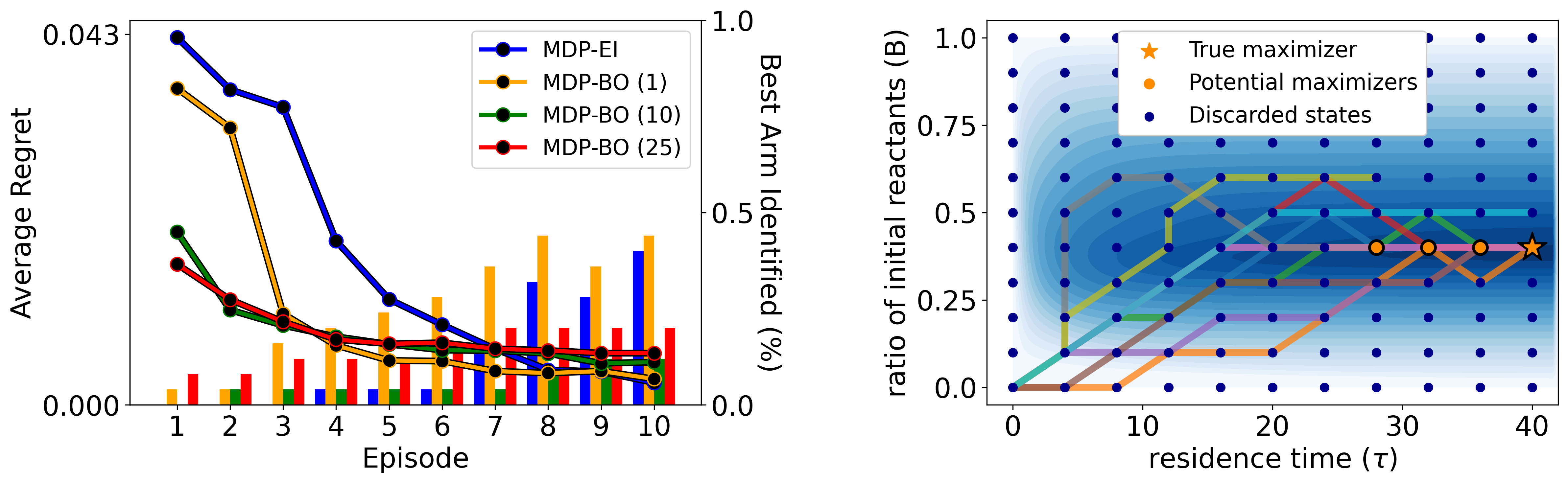
Figure 2: The Knorr pyrazole synthesis experiment. On the left, we show the quantitative results. The line plots denote the best prediction regret, while the bar charts denote the percentage of runs that correctly identify the best arm at the end of each episode. On the right, we show ten paths in different colours chosen by the algorithm. The underlying black-box function is shown as the contours, and we can see the discretization as dots. We can see four remaining potential maximizers (in orange), which includes the true one (star). Notice all paths are non-decreasing in residence time, following the transition constraints.

Sections 5.1 – 5.3 showcase real-world applications under mixed transitions constraints, using the discrete version of the algorithm. Section 5.4 benchmarks against other algorithms in the continuous setting, where we consider the additive transition model of Section 4.1 with $A=B=\mathbf{I}$. We include additional results in Appendix A.

We implemented all algorithms ourselves to ensure a fair comparison by using the same modeling and optimization sub-routines for all algorithms. We selected reasonable GP hyper-parameters for each benchmark and fixed them during the optimization; all algorithms use the same ones. In discrete problems, we report the proportion of reruns that succeed at best-arm identification. For continuous benchmarks, we report inference regret at each iteration: $\text{Regret}_{t}=f(x_{*})-f(x_{\mu,t})$, where $x_{\mu,t}=\operatorname*{arg\,max}_{x\in\mathcal{X}}\mu_{t}(x)$.

Baselines. For discrete examples, we consider end-point and monotonicity constraints, which, to our best knowledge, have never been considered in BayesOpt. Therefore, we create a baseline that replaces the gradient in Eq. (12) with Expected Improvement (referred to as MDP-EI). To understand the benefit of changing the number of components in $\pi_{\operatorname{mix}}$, we compare multiple variants of our algorithm, MDP-BO ($N$) ($N=1,10,25$). In the synthetic continuous benchmarks, we use a single mixture component for our algorithm, and for the maximization set we consider Thompson Sampling (MDP-BO-TS ($K$)) and Upper Confidence Bound (MDP-BO-UCB ($K$)), where $K$ denotes the number of maximizers. We compare against truncated SnAKe (TrSnaKe) (Folch et al., 2023b), which minimizes movement distance, and against local search region-constrained BayesOpt or LSR (Paulson et al., 2023).

5.1 Knorr pyrazole synthesis

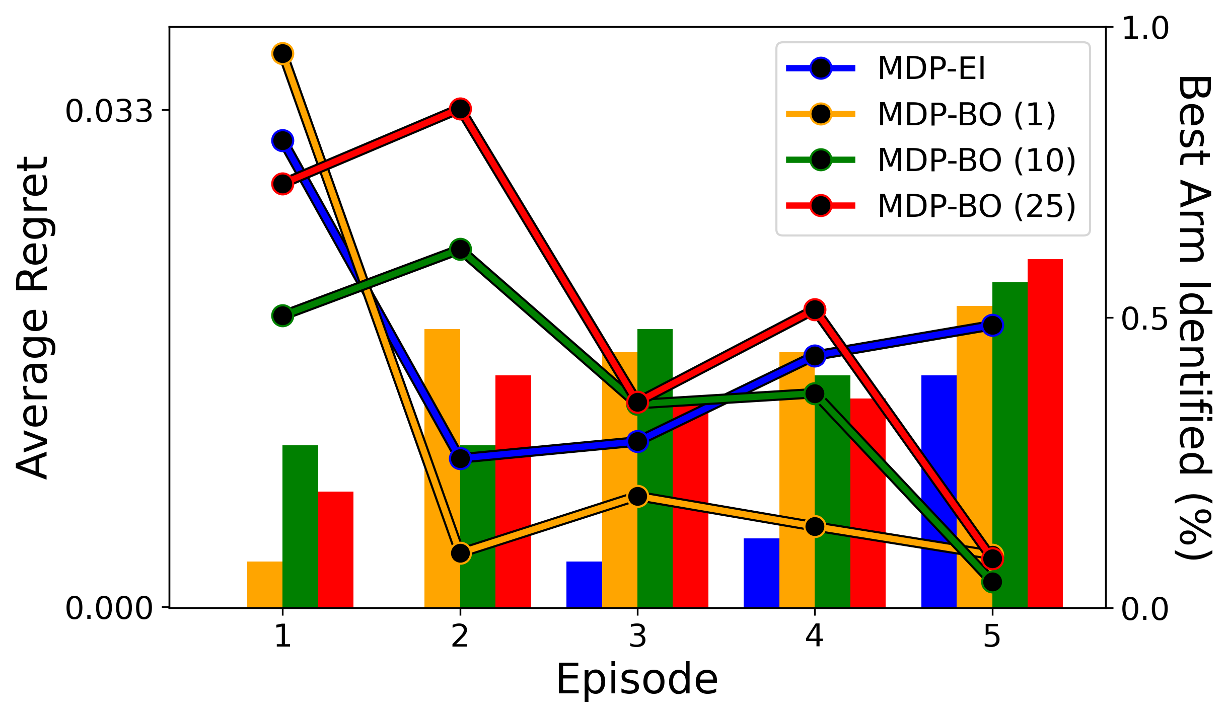
Figure 3: Results of the Lake Ypacarai experiment. The line plots denote the best prediction regret, while the bar charts denote the percentage of runs that correctly identify the best arm at the end of each episode.

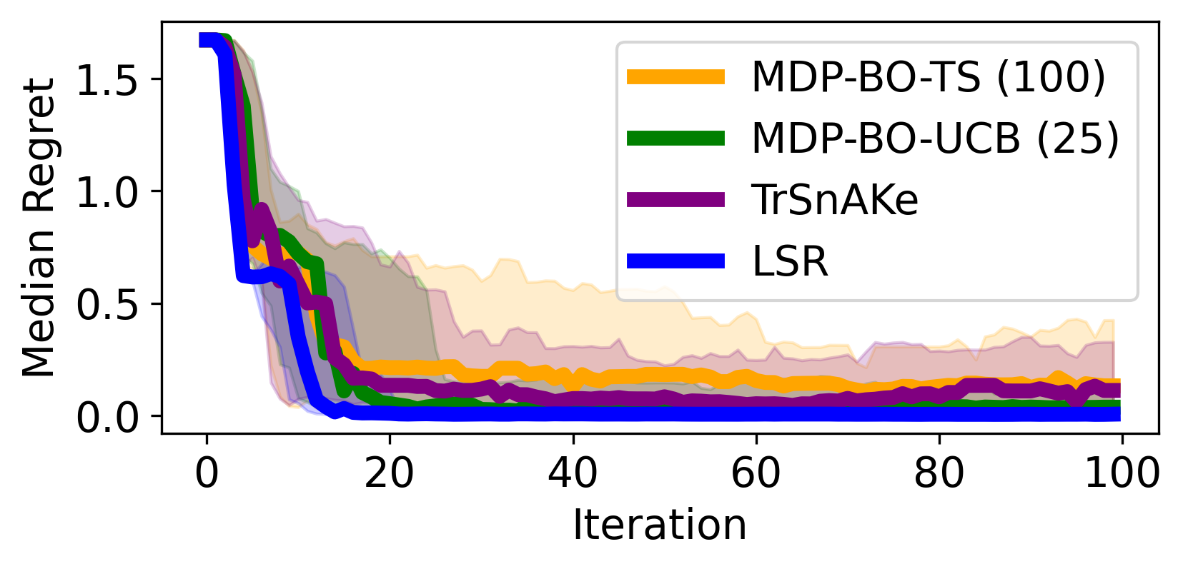
(a) Michaelwicz 3D. (synch)

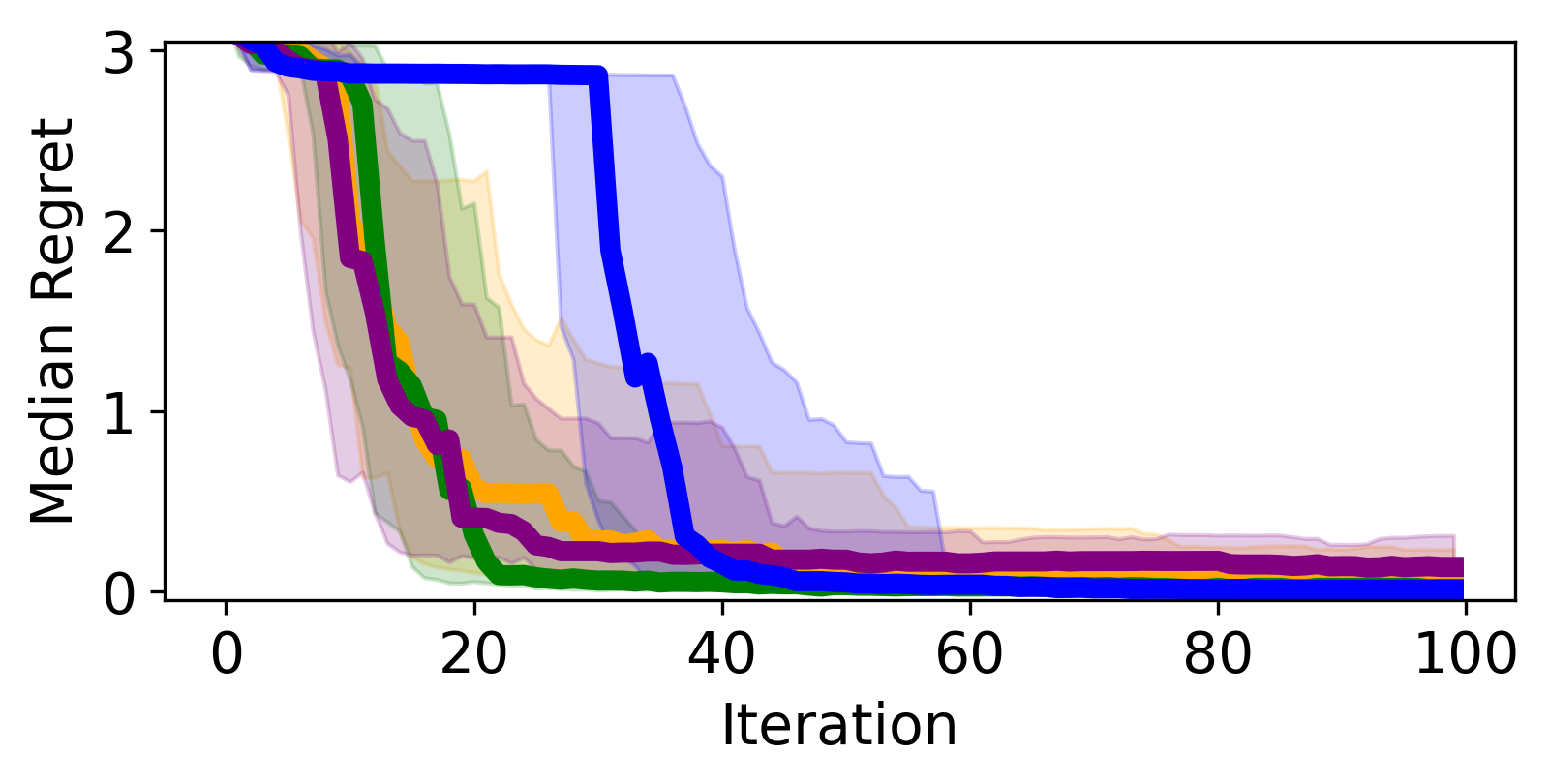
(b) Hartmann 3D. (synch)

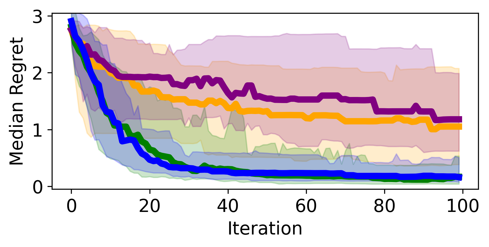
(c) Hartmann 6D. (synch)

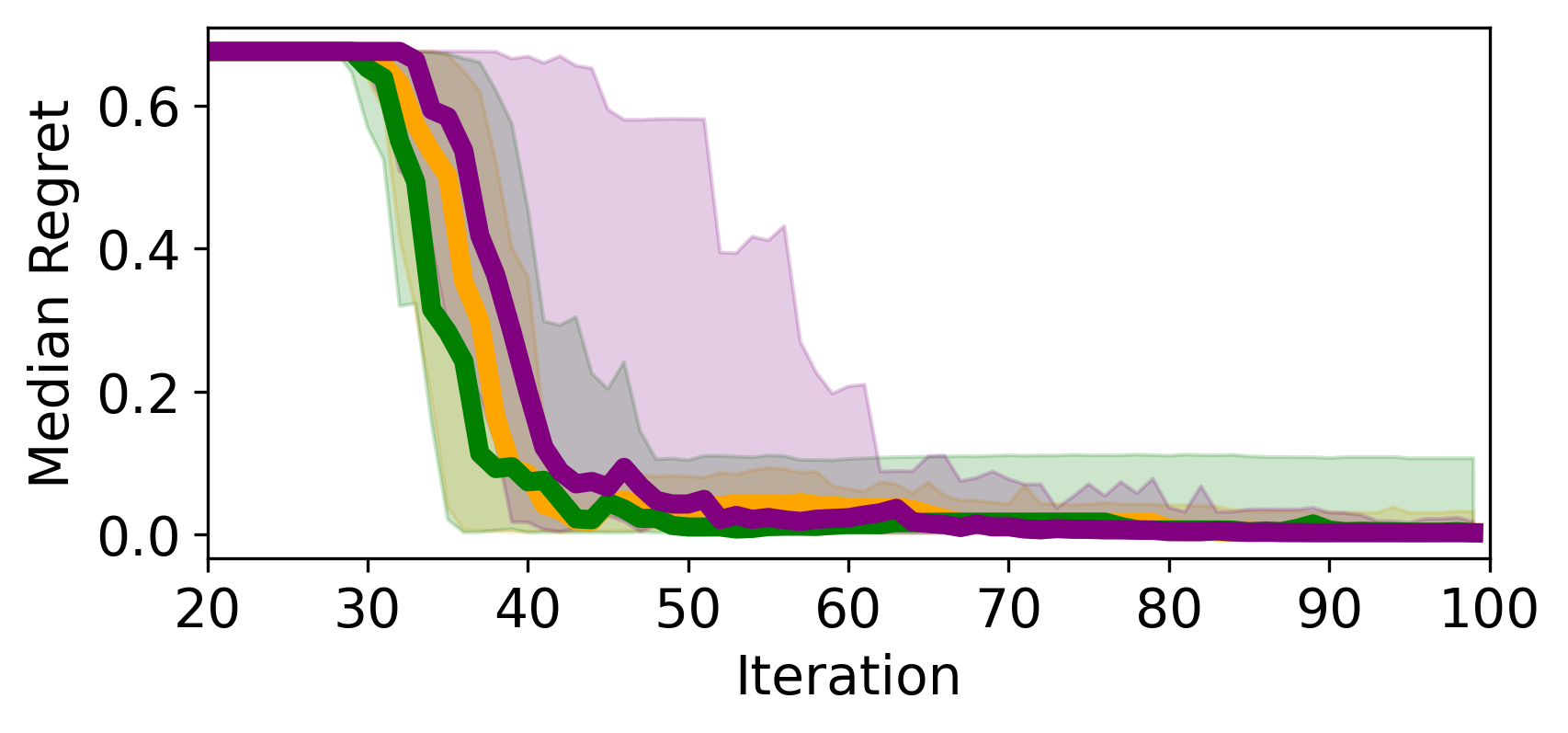
(d) Michalewicz 2D. (asynch)

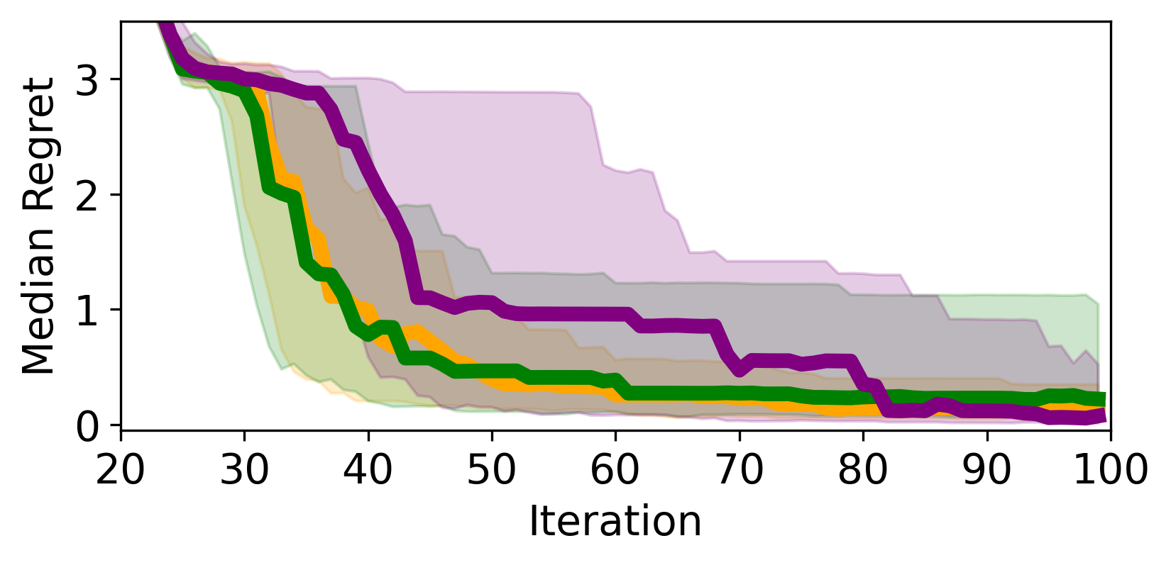
(e) Hartmann 3D. (asynch)

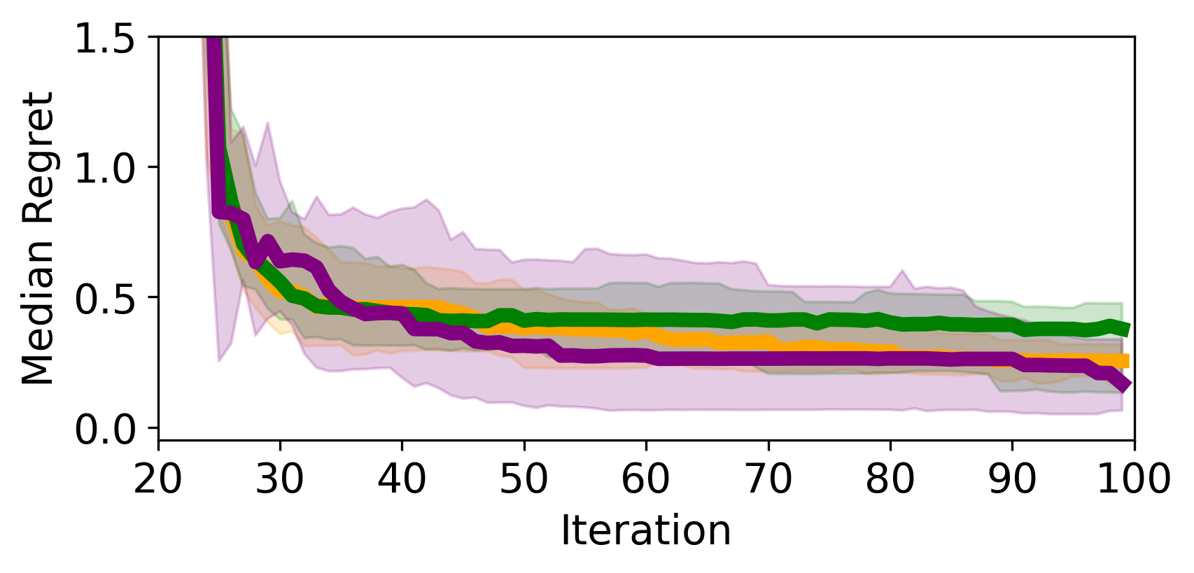
(f) SnAr 4D. (asynch)

Figure 4: Results of experiments on the asynchronous and synchronous benchmarks. We plot the median predictive regret and the 10% and 90% quantiles. For the asynchronous experiments, we can see that the paths taken by MDP-BO-TS are more consistent, and the final performance is comparable to TrSnAKe. While in the asynchronous setting, we found creating the maximization set using Thompson Sampling gave a stronger performance, in the synchronous setting, we can see UCB is preferred. We find LSR gives a very strong performance, comparable to MDP-BO-UCB in almost all benchmarks.

Schrecker et al. (2023) investigated Knorr pyrzole synthesis in transient flow reactors. and found that the typically-used, oversimplified model could be improved with more complicated kinetics. This task assumes that we only have access to the simplified model, but need to perform BayesOpt on the true model (with complicated kinetics). This discrepancy introduces a model mismatch between the oversimplified kinetics and the true model.

We seek to optimize the final product concentration of the reaction by controlling two variables: (i) the ratio between the initial reactants, $B$, and (ii) the residence time of the reaction, $\tau$.

The kernel. It has been shown how to restrict GPs to systems of linear ODEs (Mutny & Krause, 2022; Besginow & Lange-Hegermann, 2022). The ODEs in the reaction kinetics are nonlinear, but we can linearize them and build an embedding whose inner product defines a kernel:

$$\Phi_{ode}(\tau,B)=(1-\mathcal{S}(B))y^{(1)}(\tau,B)+\mathcal{S}(B)y^{(2)}(\tau,B)$$

where $y^{(i)}(\tau,B)$ are equal to:

$$\gamma_{i}(B)\left(\frac{\lambda^{(i)}_{2}}{\lambda^{(i)}_{1}-\lambda^{(i)}_{2}}e^{\lambda^{(i)}_{1}\tau}-\frac{\lambda^{(i)}_{1}}{\lambda^{(i)}_{1}-\lambda^{(i)}_{2}}e^{\lambda^{(i)}_{2}\tau}+1\right)$$

for $i=1,2$, where $\lambda^{(i)}_{1}$ and $\lambda^{(i)}_{2}$ are eigenvalues of the linearized ODE at different stationary points, $\gamma_{1}(B)=B$, $\gamma_{2}(B)=1-B$, and $\mathcal{S}(x):=(1+e^{-\alpha_{sig}(x-0.5)})^{-1}$ is a sigmoid function. Appendix G holds the details and derivations.

The above represents only an approximation of the solution, and we must account for the model mismatch. Therefore, we add a squared exponential term to the kernel to ensure a non-parametric correction, i.e.:

$$k(\tau,B)=\alpha_{ode}k_{ode}(\tau,B)+\alpha_{rbf}k_{rbf}(\tau,B).$$ (15)

Constraints. We deploy our method under the following constraints, which are determined by the flow reactor:

• We cannot change either $B$ or $\tau$ by more than 0.1.

• Decreasing the flow rate of a reactor can be easily achieved. However, increasing the flow rate can lead to inaccurate readings. A lower flow rate leads to higher residence time, so we impose that $\tau$ must be non-decreasing.

Figure 2 shows examples of paths satisfying the transition constraints. The paths are not space-filling and avoid sub-optimal areas because of our choice of kernel. We run the experiment with episodic feedback, for ten episodes of length ten each, starting each episode at $(\tau,B)=(0,0)$. Figure 2 shows that the best-performing algorithm is MDP-BO with a single component (one Frank-Wolfe step). Adding more components improves the early regret, but we struggle to identify the optimal arm at the end. MDP-EI has the worst early performance but performs well towards the end.

5.2 Monitoring Lake Ypacarai

Samaniego et al. (2021) investigated automatic monitoring of Lake Ypacarai. Folch et al. (2022) and Yang et al. (2023) benchmarked different BayesOpt algorithms for the task of finding the largest contamination source in the lake. We introduce an alternative benchmark considering local transition constraints by creating an alternative version of the lake containing obstacles that limit movement (see Figure 1). Such obstacles in environmental monitoring may include islands in bodies of water, safety zones for swimmers, or protected areas for animals.

We add initial and final state constraints. As an example, we might ask the boat to finish at the maintenance port. We focus on episodic feedback, where each episode consists of 50 iterations. Results can be seen in Figure 3. MDP-EI struggles to identify the maximum contamination for the first few episodes. On the other hand, our method correctly identifies the maximum in approximately 50% of the runs by episode two and achieves better regret.

5.3 Free-electron laser: Transition-driven corruption

Apart from hard constraints, we can apply our framework to state-dependent BayesOpt problems. For example, the magnitude of noise $\epsilon$ may depend on the transition. This occurs in systems observing equilibration constraints such as a free-electron laser (Kirschner et al., 2022). Using the simplified simulator of this laser (Mutný et al., 2020), we use our framework to model heteroscedastic noise depending on the difference between the current and next state, $\sigma^{2}(x,x^{\prime})=s(1+w||x-x^{\prime}||_{2})$. By choosing $\mathcal{A}=\mathcal{X}$, we rewrite the problem as $\sigma(s,a)=s(1+w||x-a||_{2})$. The larger the move, the more noisy the observation. This creates a problem, where the BayesOpt needs to balance between informative actions and movement, which can be directly implemented in the objective (9) via the matrix $\mathbf{V}(d_{\pi})=\sum_{x,a\in\mathcal{X}}d_{\pi}(x,a)\frac{1}{\sigma^{2}(x,a)}\Phi(x)\Phi(x)^{\top}+\lambda\mathbf{I}$. Figure 9 in Appendix C.2 reports the comparison between worst-case stateless BO and our algorithm. Our approach substantially improves performance.

5.4 Synthetic Benchmarks

We benchmark on a variety of classical BayesOpt problems while imposing local movement constraints and considering both immediate and asynchronous feedback (by introducing an observation delay of 25 iterations). We also include the chemistry SnAr benchmark, from Summit (Felton et al., 2021), which we treat as asynchronous as per Folch et al. (2022). Results are in Figure 4. In the synchronous setting, we found using the UCB maximizer criteria for MDP-BO yields the best results. We also found that LSR performs very competitively on many benchmarks, frequently matching the performance of MDP-BO-UCB. In the asynchronous setting, we find the Thompson Sampling variant of MDP-BO performs best. Our method and TrSnAKe appear to be competitive in all benchmarks. However, we do see that our method is less stochastic and has less variance in the chosen paths, which can be seen by looking at the quantiles.

6 Conclusion

We considered transition-constrained BayesOpt problems arising in physical sciences, such as chemical reactor optimization, that require careful planning to reach any system configuration. We focused on maximizer identification. We reformulated the problem with transition constraint using the framework of Markov decision processes (MDPs) and utilizing novel results in best-arm identification and experiment design to construct a tractable algorithm for provably and efficiently solving these problems using dynamic programming and model predictive control sub-routines. Further work could address the continuous variant of the framework to deal with more general transition dynamics.

Appendix A Additional Empirical Results

A.1 Constrained Ypacarai

We also run the Ypacarai experiment with immediate feedback. To increase the difficulty, we used large observation noise, $\sigma^{2}=0.01$. The results can be seen in Figure 5. The early performance of MDP-EI is much stronger, however, it gets overtaken by our algorithm from episode three onwards, and gives the worst result at the end, as it struggles to identify which of the two optima is the global one.

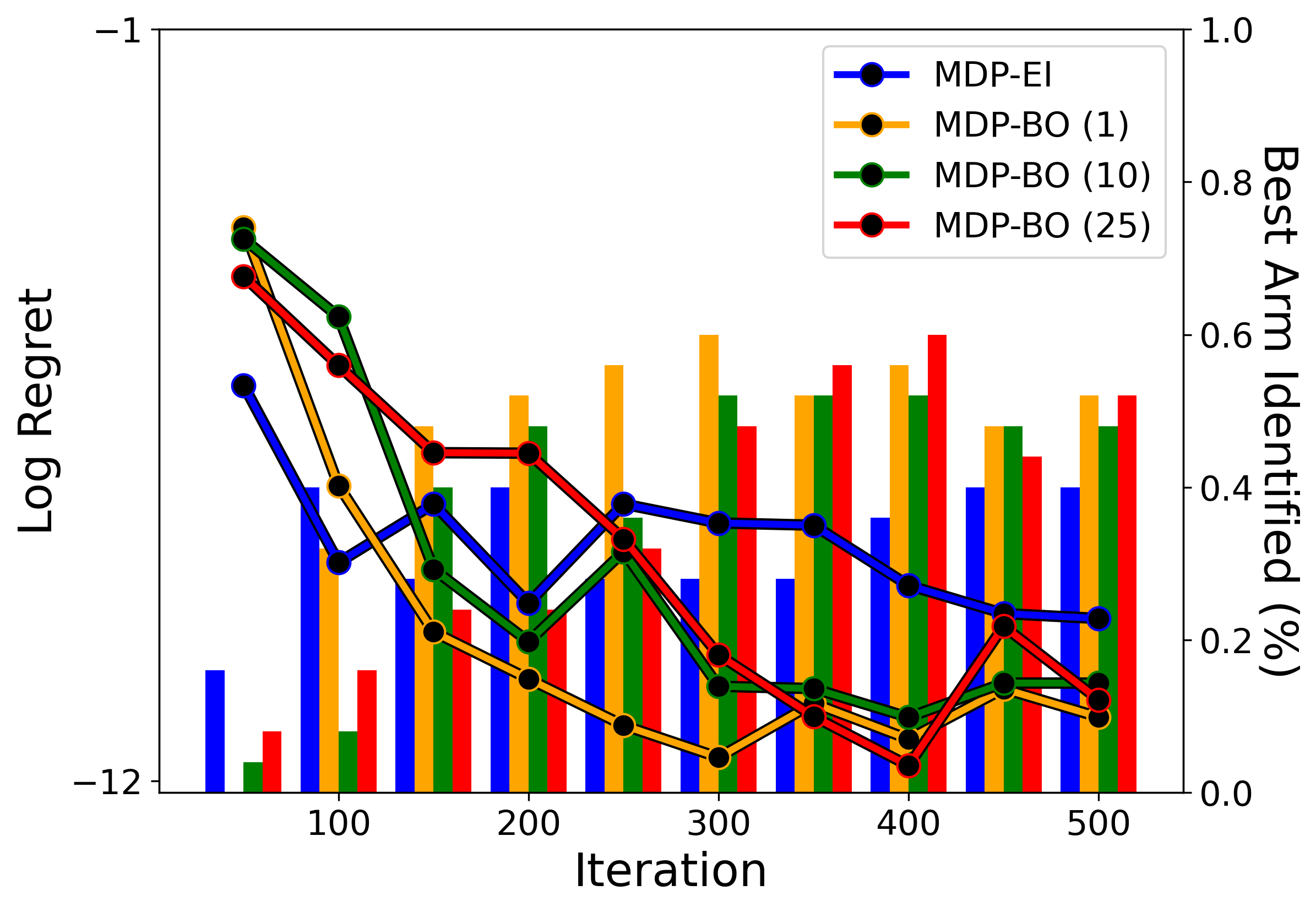
Figure 5: High noise constrained Ypacari experiment with immediate feedback.

A.2 Knorr pyrazole synthesis

We also include results for the Knorr pyrazole synthesis with immediate feedback. In this case we observe very strong early performance from MDP-BO(1), but by the end all methods are comparable.

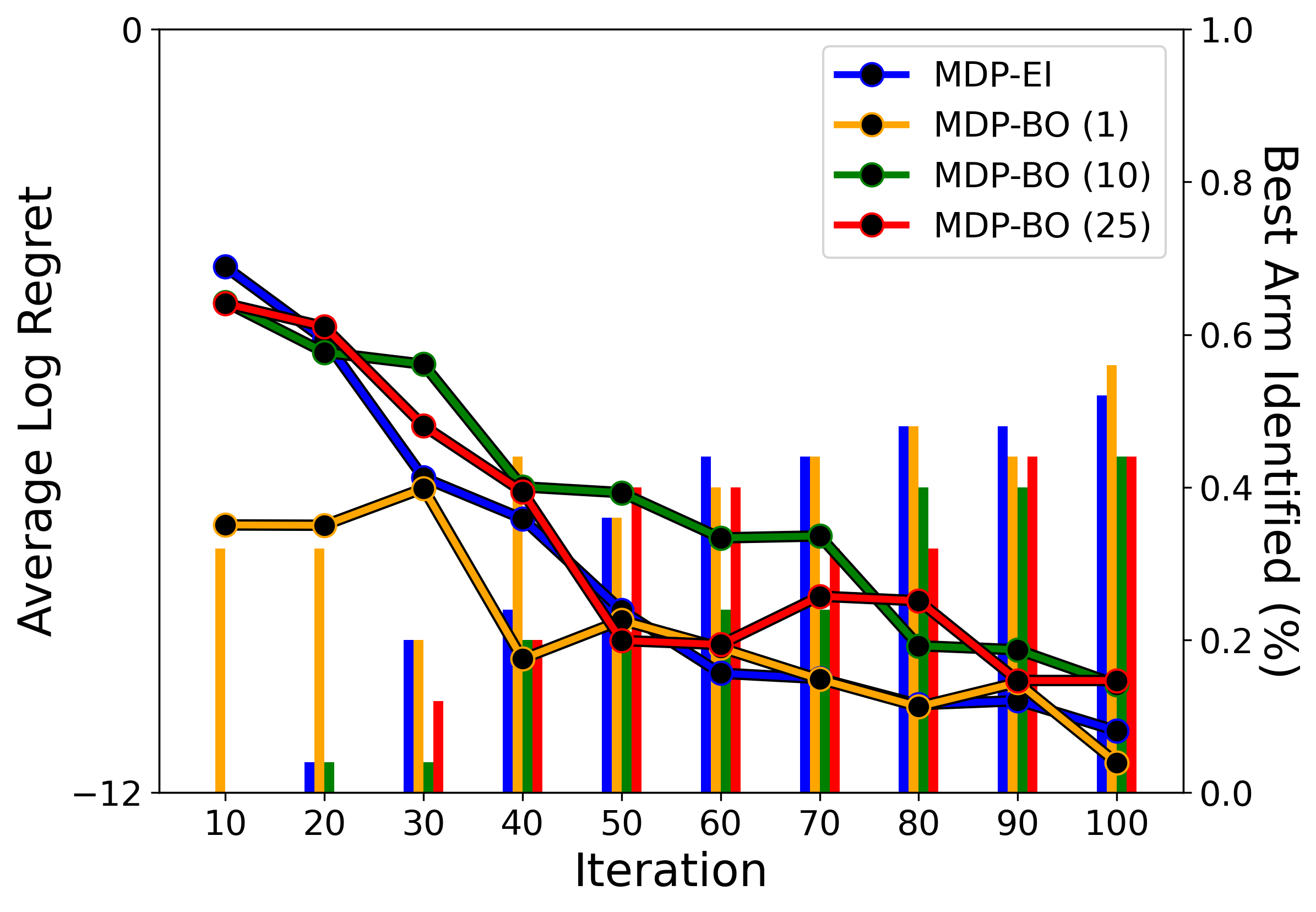
Figure 6: Knorr pyrazole synthesis with immediate feedback

A.3 Additional synthetic benchmarks

Finally, we also include additional results on more synthetic benchmarks for both synchronous and asynchronous feedback. The results are shown in Figures 7 and 8. The results back the conclusions in the main body. All benchmarks do well in 2-dimensions while highlighting further that MDP-BO-UCB and LSR can be much stronger in the synchronous setting than Thompson Sampling planning-based approaches (with the one exception of the Levy function).

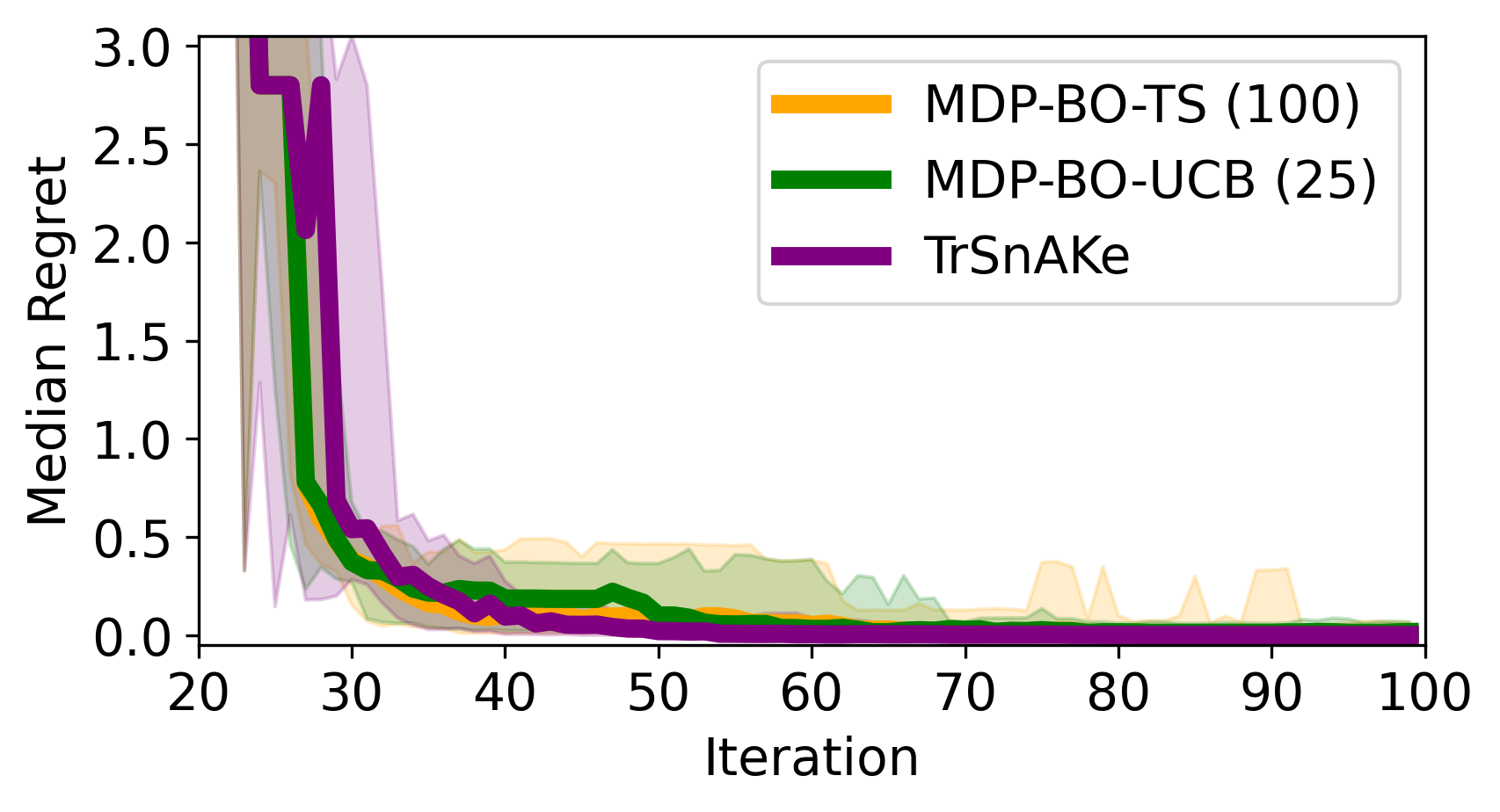
(a) Branin 2D. (asynch)

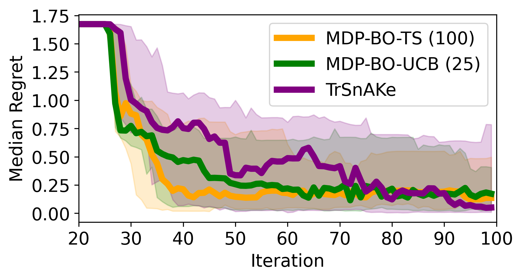
(b) Michaelwicz 3D. (asynch)

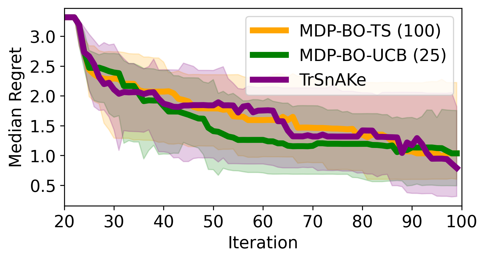
(c) Hartmann 6D. (asynch)

Figure 7: Additional asynchronous results.

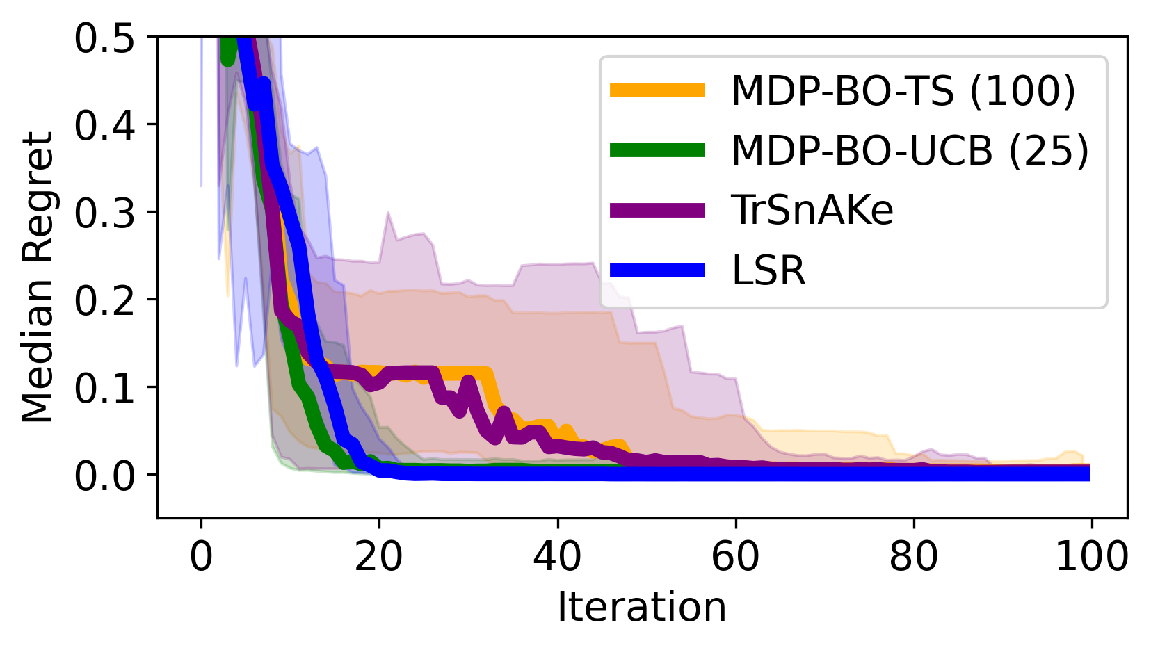
(a) Branin 2D.

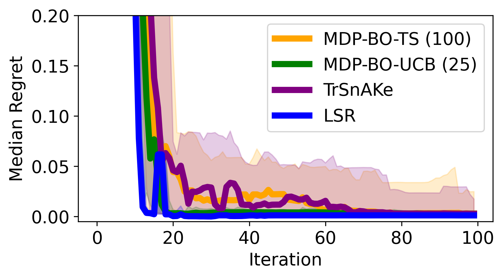
(b) Michaelwicz2D.

(c) Levy4D.

Figure 8: Additional synchronous results.

Appendix B Approximation of Gaussian Processes

Let us now briefly summarize the Nyström approximation Williams & Seeger (2000); Yang et al. (2012). Given a kernel $k(\cdot,\cdot)$, and a data-set $X$, we can choose a sub-sample of the data $\hat{x}_{1},...,\hat{x}_{m}$. Using this sample, we can create a low $r$-rank approximation of the full kernel matrix

$$\hat{K}_{r}=K_{b}\hat{K}^{\dagger}K_{b}$$

where $K_{b}=[k(x_{i},\hat{x}_{j})]_{N\times m}$, $\hat{K}=[k(\hat{x}_{i},\hat{x}_{j})]_{m\times m}$ and $K^{\dagger}$ denotes the pseudo-inverse operation. We can then define the Nyström features as:

$$\phi_{n}(x)=\hat{D}_{r}^{-1/2}\hat{V}_{r}^{T}(k(x,x_{1}),...,k(x,x_{m}))^{T},$$ (16)

where $\hat{D}_{r}$ is the diagonal matrix of non-zero eigenvalues of $\hat{K}_{r}$ and $\hat{V}_{r}$ the corresponding matrix of eigenvectors. It follows that we obtain a finite-dimensional estimate of the GP:

$$f(x)\approx\Phi(x)^{T}\theta$$ (17)

where $\Phi(x)=(\phi_{1}(x),\dots\phi_{m}(x))^{T}$, and $\theta$ are weights with a Gaussian prior.

Appendix C Implementation details and Ablation study

In this section we provide implementation details, and show some studies into the effects of specific hyper-parameters. We note that the implementation code will be made public after public review.

C.1 Benchmark Details

For all benchmarks, aside from the knorr pyrazole synthesis example, we use a standard squared exponential kernel for the surrogate Gaussian Process:

$$k_{rbf}(x,x^{\prime})=\sigma_{rbf}^{2}\exp\left(-\frac{(x-x^{\prime})^{2}}{2\ell_{rbf}}\right)$$

where $\sigma_{rbf}^{2}$ is the prior variance of the kernel, and $\ell_{rbf}$ the kernel. We fix the values of all the hyper-parameters a priori and use the same for all algorithms. The hyper-parameters for each benchmarks are included in Table 1.

For the knorr pyrazole synthesis example, we further set $\alpha_{ode}=0.6$, $\alpha_{rbf}=0.001$, $k_{1}=10$, $k_{2}=874$, $k_{3}=19200$, $\alpha_{sig}=5$. Recall we are using a finite dimensional estimate of a GP such that:

$$f(x)\approx\omega_{ode}\Phi_{ode}(x)+\sum_{i=1}^{M}\omega_{rbf,i}\Phi_{rbf}(x)$$ (18)

in this case we set a prior to the ODE weight such that $\omega_{ode}\sim\mathcal{N}(0.6,0.0225)$. This is incorporating two key pieces of prior knowledge that (a) the product concentration should be positive, and (b) we expect a maximum product concentration between 0.15 and 0.45.

The number of features for each experiment, $M$, is set to be $M=|\mathcal{X}|$ in the discrete cases and $M=\min\left(2^{5+d},512\right)$ where $d$ is the problem dimensionality.

In the case of Local Search Region BayesOpt (LSR) (Paulson et al., 2023) we set the exploration hyper-parameter to be $\gamma=0.01$ in all benchmarks.

Table 1: Benchmark and hyper-parameter information. $\Delta_{max}$ represents the size of the box constraints in the traditional benchmarks. For the synchronous benchmarks and for SnAr we used a noise level of $\sigma^{2}=0.001$. For the asynchronous benchmarks, and the knorr pyrazole example we used $\sigma^{2}=0.0001$. For the Ypacarai example we used $\sigma^{2}=0.001$ and $\sigma^{2}=0.01$ for the episodic and immediate feedback respectively.

Benchmark Name	$\Delta_{max}$	Variance $\sigma_{rbf}$	Lengthscale $\ell_{rbf}$
Knorr pyrazole	–	0.001	0.1
Constrained Ypacarai	–	1	0.2
Branin2D	0.05	0.6	0.15
Hartmann3D	0.1	2.0	0.13849
Hartmann6D	0.2	1.7	0.22
Michaelwicz2D	0.05	0.35	0.179485
Michaelwicz3D	0.1	0.85	0.179485
Levy4D	0.1	0.6	0.14175
SnAr	0.1	0.8	0.2

C.2 Free-electron Laser

We use the simulator from Mutný et al. (2020) that optimizes quadrupole magnet orientations for our experiment with varying noise levels. We use a 2-dimensional variant of the simulator. We discretize the system on $10\times 10$ grid and assume that the planning horizon $H=100$. The simulator itself is a GP fit with $\gamma=0.4$, hence we use this value. Then we make a choice that the noise variance is proportional to the change made as $\sigma^{2}(x,a)=s(1+w||x-a||^{2})$, where $s=0.01$ and $w=20$. Note that $x\in[-0.5,0.5]^{2}$ in this modeling setup. This means that local steps are indeed very desired. We showcase the difference to classical BayesOpt, which uses the worst-case variance $\sigma=\sup_{x,a}s(1+w||x-a||^{2})$ for modeling as it does not take into account the state in which the system is. We see that the absence of state modeling leads to a dramatic decrease in performance as indicated by much higher inference regret in Figure 9.

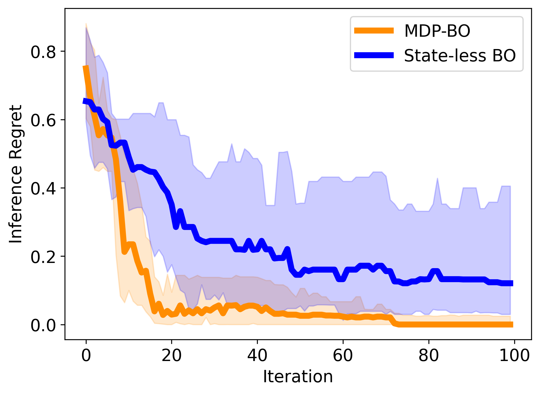
Figure 9: Free-electron laser simulator: We depict inference regret over 20 reruns (with standard quantiles) of two algorithms. Classical BayesOpt does not keep track of the state and hence incurs large noise corruption when making a large step. Our MDP-based planning takes the noise of a step into account, and ensures small enough steps are made to be informative.

C.3 Ablation Study

We explore the effect of the number of maximizers, $K$, in the maximization sets $\mathcal{Z}_{cont}^{(TS)}$ and $\mathcal{Z}_{cont}^{(UCB)}$. Overall we found the performance of the algorithm to be fairly robust to the size of the set in all benchmarks, with a higher $K$ generally leading to a little less spread in the performance.

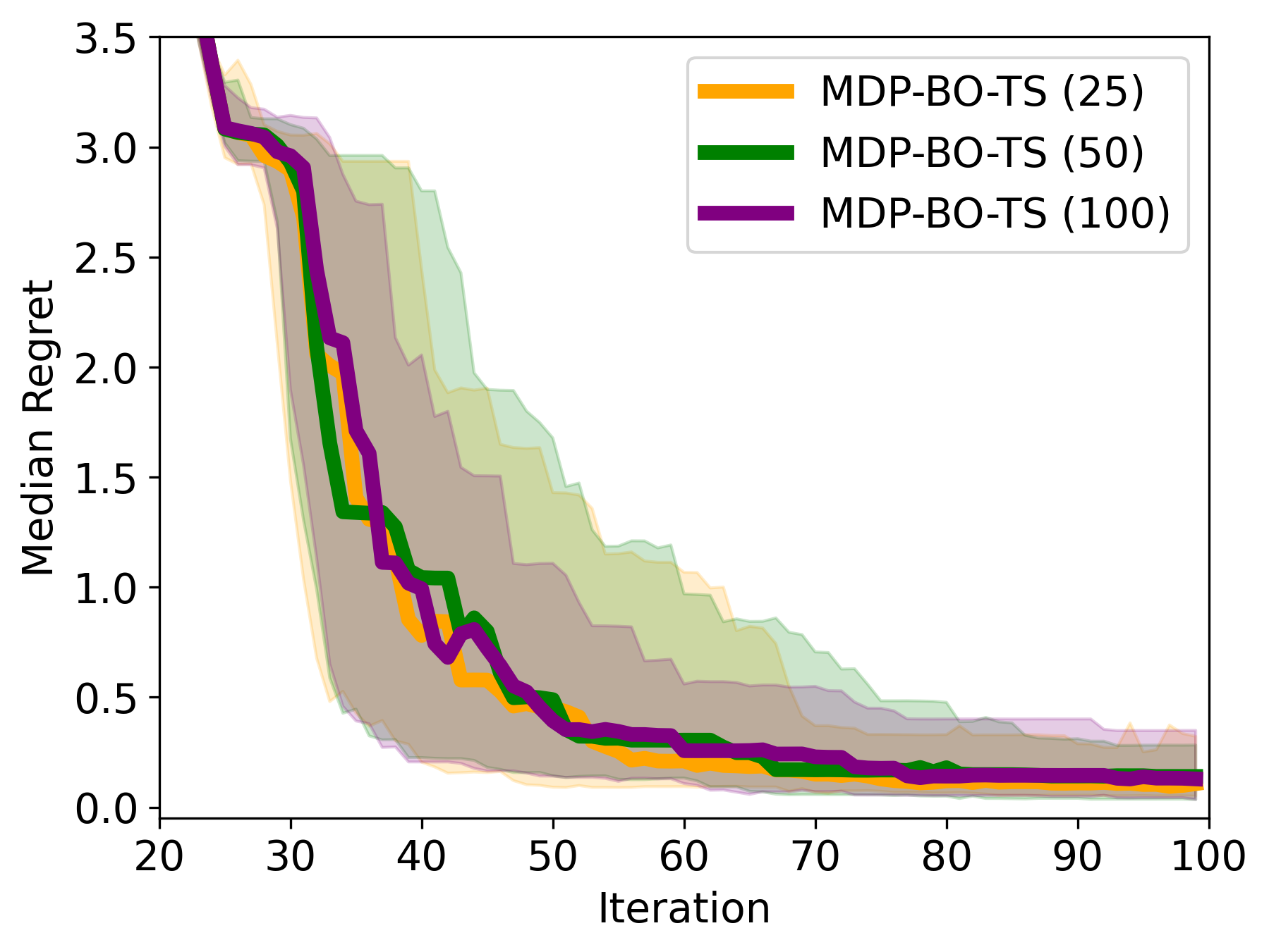
Figure 10: Ablation study into the size of the Thompson Sampling maximization set in the asynchronous Hartmann3D function. We can see that the performance of the algorithm is very similar for all values of $K=25,50,100$.

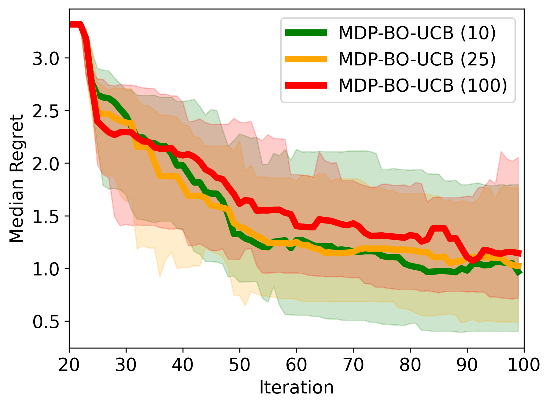
(a) Hartmann6D (asynch).

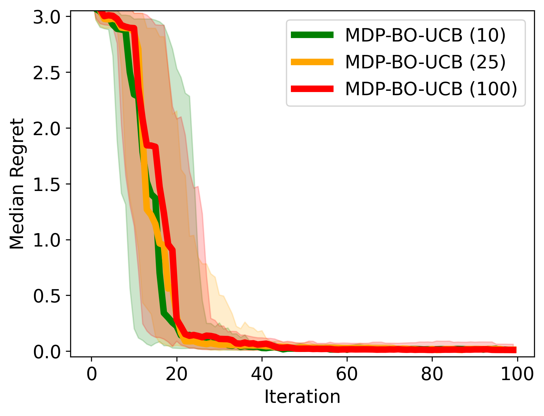
(b) Hartmann3D.

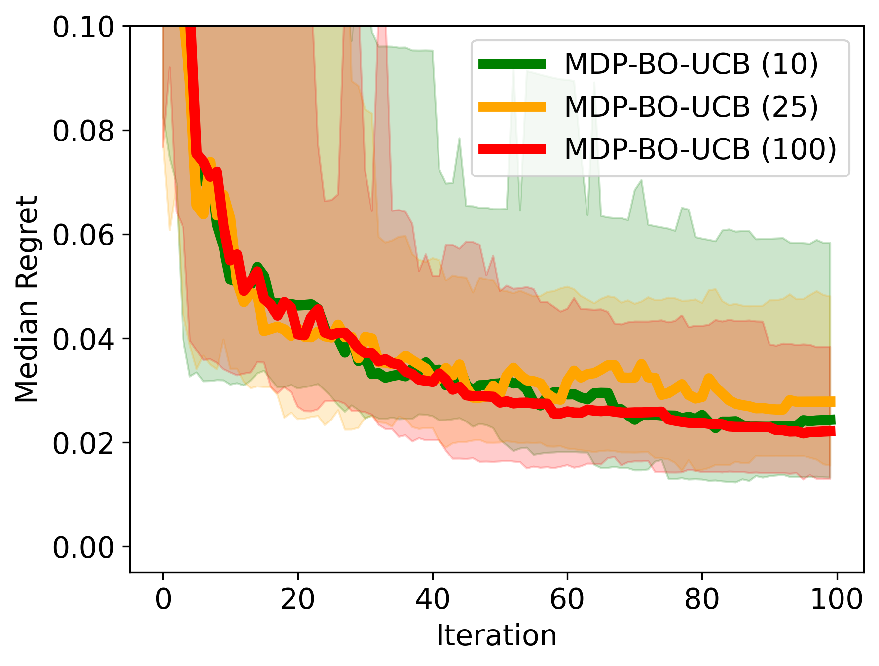
(c) Levy4D.

Figure 11: Ablation study into the size of the UCB maximization set in a variety of benchmarks. We can see that the performance of the algorithm is very similar for all values of $K=10,25,100$.

Appendix D $\mathcal{XY}$-allocation vs $\mathcal{G}$-allocation

Our objective is motivated by hypothesis testing between different arms (options) $z$ and $z^{\prime}$. In particular,

$$U(d)=\max_{z^{\prime},z\in\mathcal{Z}}\text{Var}[f(z)-f(z^{\prime})|d_{\mathbf{X}}].$$ (19)

One could maximize the information of the location of the optimum, as it has a Bayesian interpretation. This is at odds in frequentist setting, where such interpretation does not exists. Optimization of information about the maximum has been explored before, in particular via information-theoretic acquisition functions (Hennig & Schuler, 2012; Hernández-Lobato et al., 2014; Tu et al., 2022; Hvarfner et al., 2022). However, good results (in terms of regret) have been achieved by focusing only on yet another surrogate to this, namely, the value of the maximum (Wang & Jegelka, 2017). This is chiefly due to problem of dealing with the distribution of $f(x^{\star})$. Defining a posterior value for $f(z)$ is easy. Using, this and the worst-case perspective, an alternative way to approximate the best-arm objective, could be:

$$\tilde{U}(d)=\max_{z\in\mathcal{Z}}\text{Var}[f(z)|\mathbf{X}_{d}].$$ (20)

What are we losing by not considering the differences? The original objective corresponds to the $\mathcal{XY}$-allocation in the bandits literature. The modified objective will, in turn, correspond to the $\mathcal{G}$-allocation, which has been argued can perform arbitrarily worse as it does not consider the differences, e.g. see Appendix A in Soare et al. (2014). We nonetheless implemented the algorithm with objective (20), and found the results to be as expected: performance was very similar in general, however in some cases not considering the differences led to much poorer performance. As an example, see Figure 12 for results on the synchronous Branin2D benchmark.

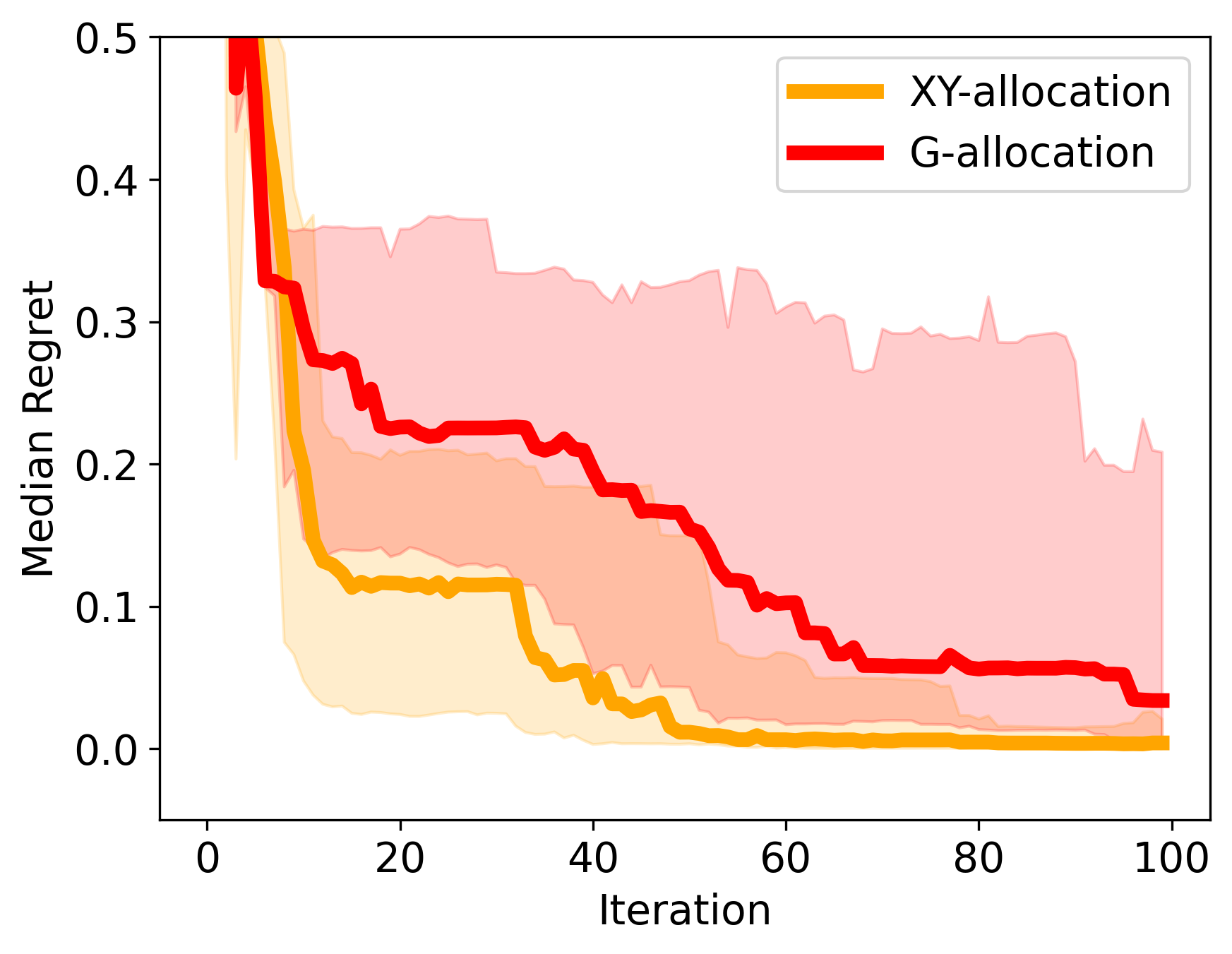
Figure 12: Comparison of using $\mathcal{XY}$-allocation against $\mathcal{G}$-allocation as the basis for the objective. In both cases the maximization sets were created using Thompson Sampling. Overall the performances were often similar, however in a few examples, such as Branin2D which we showcase here, $\mathcal{G}$-allocation performed very poorly. This is consistent with what we can expect from the bandits literature.

Appendix E Objective reformulation and linearization

For the main objective we try to optimize over a subset of $T$ trajectories $\mathbf{X}\subset\mathcal{X}^{H}$. Let be $\mathcal{X}^{H}$ be the set of sequences of inputs $\tau=(x_{1},...,x_{H})$ where they consist of states in the search space $\mathcal{X}$. Furthermore, assume there exists, in the deterministic environment, a constraint such that $x_{h+1}\in\mathcal{C}(x_{h})$ for all $h=1,...,H-1$. Then we seek to find the set $\mathbf{X}_{*}$, consisting of $T$ trajectories (possibly repeated), such that we solve the constrained optimization problem:

$$\mathbf{X}_{*}=\operatorname*{arg\,min}_{\mathbf{X}\in\mathcal{X}^{H}}\max_{z,z^{\prime}\in\mathcal{Z}}\text{Var}[f(z)-f(z^{\prime})|\mathbf{X}]\quad\text{ s.t. }\quad x_{h+1}\in\mathcal{C}(x_{h})\quad\forall t=1,...,h-1$$ (21)

We define the objective as:

$$U(\mathbf{X})=\max_{z,z^{\prime}\in\mathcal{Z}}\text{Var}\left[f(z)-f(z^{\prime})|\mathbf{X}\right]$$ (22)

Our goal is to show that optimization over sequences can be simplified to state-action visitations as in Mutny et al. (2023). For this, we require that the objective depends additively involving terms $x,a$ separately. We formalize this in the next result. In order to prove the result, we utilize the theory of reproducing kernel Hilbert spaces (Cucker & Smale, 2002).

Lemma E.1 (Additivity of Best-arm Objective).

Let $\mathbf{X}$ be a collection of $t$ trajectories of length $H$. Assuming that $f\sim\mathcal{GP}(0,k)$. Assuming that $k$ has Mercer decomposition as $k(x,y)=\lambda_{k}\phi_{k}(x)\phi_{k}(y)$.

$$f(x)=\sum_{k}\phi_{k}(x)\theta_{k}\quad\theta_{k}\sim\mathcal{N}(0,\lambda_{k}).$$

Let $d_{\mathbf{X}}$ be the visitation of the states-action in the trajectories in $\mathbf{X}$, as $d_{\mathbf{X}}=\frac{1}{HT}\sum_{t=1}^{T}\sum_{x,a\in\tau_{t}}\delta_{x,a}$, where the $\delta$ represent delta function supported on $x,a$. Then optimization of the objective Eq. (21) can be rewritten as:

$$U(d_{\mathbf{X}})=\max_{z,z^{\prime}\in\mathcal{Z}}||\Phi(z)-\Phi(z^{\prime})||_{\mathbf{V}(d_{\mathbf{X}})^{-1}}^{2},$$

where $\mathbf{V}(d)=\sum_{i}\sum_{x,a\in\tau_{i}}d(x,a)\Phi(x)\Phi(x)^{\top}+\mathbf{I}/(TH)$ is a operator $\mathbf{V}(d):\mathcal{H}_{k}\rightarrow\mathcal{H}_{k}$, the norm is RKHS norm, and $\Phi(z)_{k}=\phi_{k}(z)$.

Proof.

Notice that the posterior GP of any two points $z,z^{\prime}$ is $(f(z),f(z^{\prime}))=\mathcal{N}((\mu(z),\mu(z^{\prime})),\mathbf{K}_{z,z^{\prime}})$, where $\mathbf{K}_{z,z^{\prime}}$ is posterior kernel (consult Rasmussen & Williams (2005) for details) defined via a posterior kernel $k_{\mathbf{X}}(z,z^{\prime})=k(z,z^{\prime})-k(z,\mathbf{X})(\mathbf{K}(\mathbf{X},\mathbf{X})+\sigma^{2}\mathbf{I})^{-1}k(\mathbf{X},z^{\prime})$.

Let $k_{t}(z)=\Phi(\mathbf{X})\phi(z)$. Utilizing $k(z,z^{\prime})=\Phi(z)^{\top}\Phi(z)$ (RKHS inner product) with the Mercer decomposition and the matrix inversion lemma, the above can be written as using $\mathbf{V}=\sum_{t=1}^{T}\sum{x\in\tau_{t}}\Phi(x)\Phi(x)^{\top}+\sigma^{2}\mathbf{I}_{\mathcal{H}_{k}}.$

$$k_{\mathbf{X}}(z,z^{\prime}) = k(z,z^{\prime})-k_{t}(z)^{\top}(\mathbf{K}_{\mathbf{X},\mathbf{X}}+\sigma^{2}\mathbf{I})^{-1}k_{t}(z^{\prime})$$

$$\stackrel{{\scriptstyle\text{Mercer}}}{{=}} \Phi(z)^{\top}\Phi(z^{\prime})-\Phi(z)^{\top}\Phi(\mathbf{X})^{\top}(\Phi(\mathbf{X})\Phi(\mathbf{X})^{\top}+\sigma^{2}\mathbf{I})^{-1}\Phi(\mathbf{X})\Phi(z^{\prime})$$

$$\stackrel{{\scriptstyle\text{Lemma \ref{lemma:matrix_inversion_lemma}}}}{{=}} \Phi(z)^{\top}\Phi(z^{\prime})-\Phi(z)^{\top}\mathbf{V}^{-1}(\mathbf{V}-\mathbf{I}\sigma^{2})\Phi(z^{\prime})$$

$$= \Phi(z)^{\top}\mathbf{V}^{-1}\mathbf{V}\Phi(z^{\prime})-\Phi(z)^{\top}\mathbf{V}^{-1}(\mathbf{V}-\mathbf{I}\sigma^{2})\Phi(z^{\prime})$$

$$= \Phi(z)^{\top}\mathbf{V}^{-1}(\mathbf{V}-\mathbf{V}+\mathbf{I}\sigma^{2})\Phi(z^{\prime})$$

Leading finally to:

$$k_{\mathbf{X}}(z,z^{\prime})=\sigma^{2}\Phi(z)^{\top}\left(\sum_{t=1}^{T}\sum_{x\in\tau_{t}}\Phi(x)\Phi(x)^{\top}+\sigma^{2}\mathbf{I}_{\mathcal{H}_{k}}\sigma^{2}\right)^{-1}\Phi(z^{\prime}).$$ (23)

Let us calculate $\text{Var}[f(z)-f(z^{\prime})|\mathbf{X}]$. The variance does not depend on the mean. Hence,

$$\text{Var}\left[f(z)-f(z^{\prime})|\mathbf{X}\right] = \text{Var}(f(z))-\text{Var}(f(z^{\prime}))-2\text{Cov}(f(z),f(z^{\prime}))$$

$$= k_{\mathbf{X}}(z,z)+k_{\mathbf{X}}(z^{\prime},z^{\prime})-2k_{\mathbf{X}}(z,z^{\prime})$$

$$\stackrel{{\scriptstyle\eqref{eq: relation}}}{{=}} (\Phi(z)-\Phi(z^{\prime}))\left(\sum_{t=1}^{T}\sum_{x\in\tau_{t}}\Phi(x)\Phi(x)^{\top}+\mathbf{I}_{\mathcal{H}_{k}}\sigma^{2}\right)^{-1}(\Phi(z)-\Phi(z^{\prime}))$$

$$= (\Phi(z)-\Phi(z^{\prime}))\left(\frac{TH}{TH}\sum_{t=1}^{T}\sum_{x\in\mathcal{X}}\#(x\in\tau_{t})\Phi(x)\Phi(x)^{\top}+\mathbf{I}_{\mathcal{H}_{k}}\sigma^{2}\right)^{-1}(\Phi(z)-\Phi(z^{\prime}))$$

$$= TH(\Phi(z)-\Phi(z^{\prime}))\left(TH\sum_{x\in\mathcal{X}}d(\mathbf{X})\Phi(x)\Phi(x)^{\top}+\frac{\mathbf{I}_{\mathcal{H}_{k}}}{TH}\sigma^{2}\right)^{-1}(\Phi(z)-\Phi(z^{\prime}))$$

The symbol $\#$ counts the number of occurrences. Notice that we have been able to show that the objective decomposes over state-action visitations as $d_{\mathbf{X}}$ decomposes over their visitations

∎

Note that the objective equivalence does not imply that optimization problem in Eq. (21) is equivalent to finding,

$$d_{*}=\operatorname*{arg\,min}_{d_{\pi}\in\mathcal{D}}\max_{z,z^{\prime}\in\mathcal{Z}}||\Phi(z)-\Phi(z^{\prime})||_{\mathbf{V}(d_{\pi})^{-1}}.$$ (24)

In other words, optimization over trajectories and optimization over $d_{\pi}\in\mathcal{D}$ is not equivalent. The latter is merely a continuous relaxation of discrete optimization problems to the space of Markov policies. It is in line with the classical relaxation approach addressed in experiment design literature with a rich history, e.g., Chaloner & Verdinelli (1995). For introductory texts on the topic, consider Pukelsheim (2006) for the statistical perspective and Boyd & Vandenberghe (2004) for the optimization perspective. However, as Mutny et al. (2023) points out, optimization of this objective does optimize objective as Eq. (21). In other words, by optimizing the relaxation with a larger budget of trajectories or horizons, we are able to decrease Eq. (21) as well.

The core difference where the two formulations differ is that there is no unique way to construct an optimal trajectory from state visitations.

For completeness, we state the auxiliary lemma.

Lemma E.2 (Matrix Inversion Lemma).

Let $\mathbf{A}\in\mathbb{R}^{n\times q}$ then

$$\mathbf{A}^{\top}(\mathbf{A}\mathbf{A}^{\top}+\rho^{2}\mathbf{I})^{-1}=(\mathbf{A}^{\top}\mathbf{A}+\rho^{2}\mathbf{I})^{-1}\mathbf{A}^{\top}.$$ (25)

Note that instead of inverting $n\times n$ matrix, we can invert a $q\times q$ matrix.

Proof.

$$\mathbf{A}^{\top}(\mathbf{A}\mathbf{A}^{\top}+\rho^{2}\mathbf{I})^{-1} \stackrel{{\scriptstyle\text{SMW}}}{{=}} \mathbf{A}^{\top}(\rho^{-2}\mathbf{I}-\rho^{-2}\mathbf{A}(\rho^{2}\mathbf{I}+\mathbf{A}^{\top}\mathbf{A})^{-1}\mathbf{A}^{\top})$$

$$= (\rho^{-2}\mathbf{I}-\rho^{-2}\mathbf{A}^{\top}\mathbf{A}(\rho^{2}\mathbf{I}+\mathbf{A}^{\top}\mathbf{A})^{-1})\mathbf{A}^{\top}$$

$$= (\rho^{-2}(\rho^{2}\mathbf{I}+\mathbf{A}^{\top}\mathbf{A})-\rho^{-2}\mathbf{A}^{\top}\mathbf{A})(\rho^{2}\mathbf{I}+\mathbf{A}^{\top}\mathbf{A})^{-1}\mathbf{A}^{\top}$$

$$= (\mathbf{A}^{\top}\mathbf{A}+\rho^{2}\mathbf{I})^{-1}\mathbf{A}^{\top}$$

∎

E.1 Linearizing the objective

To apply our method, we find ourselves having to frequently solve RL sub-problems where we try to maximize $\sum_{x,a}d(x,a)\nabla F(x,a)$. To approximately solve this problem in higher dimensions, it becomes very important to understand what the linearized functional looks like.

Remark E.3.

Assume the same black-box model as in Lemma E.1, and further assume that we have a mixture of policies $\pi_{\operatorname{mix}}$ with density $d_{\pi_{\operatorname{mix}}}$, such that there exists a set $\ \mathbf{X}_{\operatorname{mix}}\$ satisfying $d_{\pi_{\operatorname{mix}}}=\frac{1}{N}\sum_{x\in\mathbf{X}_{\operatorname{mix}}}\delta_{x}\$ for some integer $N$. Then:

$$\nabla F(d_{\pi_{\operatorname{mix}}})(x,a)\propto-\left(\text{Cov}[f(z_{*}),f(x)|\mathbf{X}_{\operatorname{mix}}]-\text{Cov}[f(z_{*}^{\prime}),f(x)|\mathbf{X}_{\operatorname{mix}}]\right)^{2}$$

where $z_{*},z_{*}^{\prime}=\operatorname*{arg\,max}_{z,z^{\prime}\in\mathcal{Z}}\text{Var}[f(z)-f(z^{\prime})]$.

Proof.

To show this, we begin by defining:

$$\Sigma_{\theta,d} =\left(\sum_{x\in\mathcal{X}}\Phi(x)\Phi(x)^{T}d(x)+\lambda\sigma^{2}I\right)^{-1}$$

$$z_{*},z_{*}^{\prime} =\operatorname*{arg\,max}_{z,z^{\prime}\in\mathcal{Z}}||\Phi(z)-\Phi(z^{\prime})||^{2}_{\Sigma_{\theta,d}}$$

$$\tilde{z}_{*} =\Phi(z_{*})-\Phi(z_{*}^{\prime})$$

It then follows, by applying Danskin’s Theorem that:

$$\nabla U(d)(x) =\nabla\tilde{z}_{*}^{T}\Sigma_{\theta,d}\tilde{z}_{*}$$

$$=\nabla\text{Tr}\left\{\tilde{z}_{*}\tilde{z}_{*}^{T}\Sigma_{\theta,d}\right\}$$

$$=\text{Tr}\left\{\tilde{z}_{*}\tilde{z}_{*}^{T}\nabla\Sigma_{\theta,d}\right\}$$

$$=-\text{Tr}\left\{\tilde{z}_{*}\tilde{z}_{*}^{T}\Sigma_{\theta,d}\Phi(x)\Phi(x)^{T}\Sigma_{\theta,d}\right\}\qquad(\text{as }\partial K^{-1}=-K^{-1}(\partial K)K^{-1}))$$

$$=-\text{Tr}\left\{\tilde{z}_{*}^{T}\Sigma_{\theta,d}\Phi(x)\Phi(x)^{T}\Sigma_{\theta,d}\tilde{z}_{*}\right\}$$

$$=-\left(\tilde{z}_{*}^{T}\Sigma_{\theta,d}\Phi(x)\right)\left(\Phi(x)^{T}\Sigma_{\theta,d}\tilde{z}_{*}\right)$$

$$\propto-\left(\text{Cov}[f(z_{*}),f(x)]-\text{Cov}[f(z_{*}^{\prime}),f(x)]\right)\left(\text{Cov}[f(x),f(z_{*})]-\text{Cov}[f(x),f(z_{*}^{\prime})]\right)$$

$$=-\left(\text{Cov}[f(z_{*}),f(x)]-\text{Cov}[f(z_{*}^{\prime}),f(x)]\right)^{2}$$

∎

Appendix F Practical Planning for Continuous MDPs

From remark E.3 it becomes clear that for decreasing covariance functions, such as the squared exponential, $\nabla F$ will consist of two modes around $z_{*}$ and $z_{*}^{\prime}$ The sub-problem seems to find a sequence that maximizes the sum of gradients, therefore the optimal solution will try to reach one of the two modes as quickly as possible. For shorter time horizons, the path will reach whichever mode is closest, and for large enough horizons, the sum will be maximized by reaching the larger of the two modes.

Therefore we can approximately solve the problem by checking the value of the sub-problem objective in (14) for the shortest paths from $x_{t-1}\rightarrow z_{*}$ and $x_{t-1}\rightarrow z_{*}^{\prime}$, which are trivial to find under the constraints in (14). Note that the paths might not necessarily be optimal, as they may be improved by small perturbations, e.g., there might be a small deviation that allows us to visit the smaller mode on the way to the larger mode increasing the overall value of the sum of gradients, however, they give us a good and quick approximation.

Appendix G Kernel for ODE Knorr pyrazole synthesis

The kernel is based on the following ODE model, which is well known in the chemistry literature and given in Schrecker et al. (2023).

$$R_{1} =k_{1}y_{2}y_{3}-k_{2}y_{4}y_{5}$$ (26)

$$R_{2} =k_{3}y_{4}$$ (27)

and then:

$$\frac{\text{d}y_{1}}{\text{d}t} =R_{2}$$

$$\frac{\text{d}y_{2}}{\text{d}t} =-R_{1}$$

$$\frac{\text{d}y_{3}}{\text{d}t} =-R_{1}$$

$$\frac{\text{d}y_{4}}{\text{d}t} =R_{1}-R_{2}$$

$$\frac{\text{d}y_{5}}{\text{d}t} =R_{1}+R_{2}$$

Our main goal is to optimize the product concentration of the reaction, which is given by $y_{1}$. We do this by sequentially querying the reaction, where we select the residence time, and the initial conditions of the ODE, in the form $y_{0}=[0,A,B,0,0]$, where $A=1-B$.

Due to the non-linearity in Eq. (26) we are unable to fit a GP to the process directly. Instead, we first linearize the ODE around two equilibrium points. The set of points of equilibrium are given by:

$$S_{1} =\left\{y_{1}=a_{1},y_{2}=b_{1},y_{3}=0,y_{4}=0,y_{5}=c_{1}|a_{1},b_{1},c_{1}\in\mathbf{R}\right\}$$

$$S_{2} =\left\{y_{1}=a_{2},y_{2}=0,y_{3}=b_{2},y_{4}=0,y_{5}=c_{2}|a_{1},b_{1},c_{1}\in\mathbf{R}\right\}$$

And the Jacobian of the system is:

$$\mathbf{J}=\begin{bmatrix}0&0&0&k_{3}&0\\ 0&-k_{1}y_{3}&-k_{1}y_{2}&k_{2}y_{5}&k_{2}y_{4}\\ 0&-k_{1}y_{3}&-k_{1}y_{2}&k_{2}y_{5}&k_{2}y_{4}\\ 0&k_{1}y_{3}&k_{1}y_{2}&-k_{2}y_{5}-k_{3}&-k_{2}y_{4}\\ 0&k_{1}y_{3}&k_{1}y_{2}&-k_{2}y_{5}+k_{3}&-k_{2}y_{4}\end{bmatrix}$$

Giving:

$$\mathbf{J}_{1}=\mathbf{J}|_{S_{1}}=\begin{bmatrix}0&0&0&k_{3}&0\\ 0&0&-k_{1}b_{1}&k_{2}c_{1}&0\\ 0&0&-k_{1}b_{1}&k_{2}c_{1}&0\\ 0&0&k_{1}b_{1}&-k_{2}c_{1}-k_{3}&0\\ 0&0&k_{1}b_{1}&-k_{2}c_{1}+k_{3}&0\end{bmatrix}$$

$$\mathbf{J}_{2}=\mathbf{J}|_{S_{2}}=\begin{bmatrix}0&0&0&k_{3}&0\\ 0&-k_{1}b_{2}&0&k_{2}c_{2}&0\\ 0&-k_{1}b_{2}&0&k_{2}c_{2}&0\\ 0&k_{1}b_{2}&0&-k_{2}c_{2}-k_{3}&0\\ 0&k_{1}b_{2}&0&-k_{2}c_{2}+k_{3}&0\end{bmatrix}$$

Unfortunately, since the matrices are singular, we do not get theoretical results on the quality of the linearization. However, linearization is still possible, with the linear systems given by:

$$\frac{\text{d}\vec{y}}{\text{d}t}=\mathbf{J}_{1}\vec{y}\qquad\qquad\frac{\text{d}\vec{y}}{\text{d}t}=\mathbf{J}_{2}\vec{y}$$

We focus on the first system for now. The matrix has the following eigenvalues:

$$\lambda_{1,2} =-\frac{1}{2}\left(b_{1}k_{1}+c_{1}k_{2}+k_{3}\pm\sqrt{b_{1}^{2}k_{1}^{2}+c_{1}^{2}k_{2}^{2}+k_{3}^{2}+2b_{1}c_{1}k_{1}k_{2}-2k_{3}(b_{1}k_{1}-c_{1}k_{2})}\right)$$

$$\lambda_{3,4,5} =0$$

Note that the three eigenvalues give us the corresponding solution based on their (linearly separable) eigenvectors:

$$v_{3}=\begin{bmatrix}1&0&0&0&0\end{bmatrix},\quad v_{4}=\begin{bmatrix}0&1&0&0&0\end{bmatrix},\quad v_{5}=\begin{bmatrix}0&0&0&0&1\end{bmatrix}$$

$$\vec{y}(t)=p_{3}v_{3}+p_{4}v_{4}+p_{5}v_{5}$$

where $p_{i}$ are constants. The behaviour of the ODE when this is not the case will depend on whether the remaining eigenvalues will be real or not. However, note:

$$b_{1}^{2}k_{1}^{2}+c_{1}^{2}k_{2}^{2}+k_{3}^{2}+2b_{1}c_{1}k_{1}k_{2}-2k_{3}(b_{1}k_{1}-c_{1}k_{2})\geq b_{1}^{2}k_{1}^{2}+k_{3}^{2}-2b_{1}k_{1}k_{3}=(b_{1}k_{1}-k_{3})^{2}\geq 0$$

and therefore all eigenvalues will always be real. Therefore we can write down the solution as:

$$\vec{y}(t)=p_{1}v_{1}e^{\lambda_{1}t}+p_{2}v_{2}e^{\lambda_{2}t}+p_{3}v_{3}+p_{4}v_{4}+p_{5}v_{5}$$

where we ignore the case of repeated eigenvalues for simplicity (this is the case where $b_{1}^{2}k_{1}^{2}+2b_{1}c_{1}k_{1}k_{2}+c_{1}^{2}k_{2}^{2}-2k_{3}(b_{1}k_{1}-c_{1}k_{2})+k_{3}^{2}$ is exactly equal to zero). We further note that the eigenvalues will be non-negative as:

$$b_{1}k_{1}+c_{1}k_{2}+k_{3} =\sqrt{(bk_{1}+c_{1}k_{2}+k_{3})^{2}}$$

$$=\sqrt{b_{1}^{2}k_{1}^{2}+c^{2}k_{2}^{2}+k_{3}^{2}+2b_{1}c_{1}k_{1}k_{2}+2c_{1}k_{2}k_{2}+2b_{1}k_{1}k_{3}}$$

$$\geq\sqrt{b_{1}^{2}k_{1}^{2}+c_{1}^{2}k_{2}^{2}+k_{3}^{2}+2b_{1}c_{1}k_{1}k_{2}+2c_{1}k_{2}k_{2}-2b_{1}k_{1}k_{3}}$$

therefore:

$$\lambda_{1}\leq\lambda_{2}\leq 0$$

which means the solutions will always be a linear combination of exponentially decaying functions of time plus constants.

The eigenvectors have the closed form:

$$v_{1}=\begin{pmatrix}1,\\ \frac{1}{2}\left(b_{1}k_{1}+c_{1}k_{2}-k_{3}+\sqrt{b_{1}^{2}k_{1}^{2}+2b_{1}c_{1}k_{1}k_{2}+c_{1}^{2}k_{2}^{2}-2(b_{1}k_{1}-c_{1}k_{2})k_{3}+k_{3}^{2}}\right)/k_{3},\\ \frac{1}{2}\left(b_{1}k_{1}+c_{1}k_{2}-k_{3}+\sqrt{b_{1}^{2}k_{1}^{2}+2b_{1}c_{1}k_{1}k_{2}+c_{1}^{2}k_{2}^{2}-2(b_{1}k_{1}-c_{1}k_{2})k_{3}+k_{3}^{2}}\right)/k_{3},\\ -\frac{1}{2}\left(b_{1}k_{1}+c_{1}k_{2}+k_{3}+\sqrt{b_{1}^{2}k_{1}^{2}+2b_{1}c_{1}k_{1}k_{2}+c_{1}^{2}k_{2}^{2}-2(b_{1}k_{1}-c_{1}k_{2})k_{3}+k_{3}^{2}}\right)/k_{3},\\ -\frac{1}{2}\left(b_{1}k_{1}+c_{1}k_{2}-3k_{3}+\sqrt{b_{1}^{2}k_{1}^{2}+2b_{1}c_{1}k_{1}k_{2}+c_{1}^{2}k_{2}^{2}-2(b_{1}k_{1}-c_{1}k_{2})k_{3}+k_{3}^{2}}\right)/k_{3}\end{pmatrix}=\begin{pmatrix}1,\\ -\lambda_{1}/k_{3}-1,\\ -\lambda_{1}/k_{3}-1,\\ \lambda_{1}/k_{3},\\ \lambda_{1}/k_{3}+2\end{pmatrix}$$

$$v_{2}=\begin{pmatrix}1,\\ \frac{1}{2}\left(b_{1}k_{1}+c_{1}k_{2}-k_{3}-\sqrt{b_{1}^{2}k_{1}^{2}+2b_{1}c_{1}k_{1}k_{2}+c_{1}^{2}k_{2}^{2}-2(b_{1}k_{1}-c_{1}k_{2})k_{3}+k_{3}^{2}}\right)/k_{3},\\ \frac{1}{2}\left(b_{1}k_{1}+c_{1}k_{2}-k_{3}-\sqrt{b_{1}^{2}k_{1}^{2}+2b_{1}c_{1}k_{1}k_{2}+c_{1}^{2}k_{2}^{2}-2(b_{1}k_{1}-c_{1}k_{2})k_{3}+k_{3}^{2}}\right)/k_{3},\\ -\frac{1}{2}\left(b_{1}k_{1}+c_{1}k_{2}+k_{3}-\sqrt{b_{1}^{2}k_{1}^{2}+2b_{1}c_{1}k_{1}k_{2}+c_{1}^{2}k_{2}^{2}-2(b_{1}k_{1}-c_{1}k_{2})k_{3}+k_{3}^{2}}\right)/k_{3},\\ -\frac{1}{2}\left(b_{1}k_{1}+c_{1}k_{2}-3k_{3}-\sqrt{b_{1}^{2}k_{1}^{2}+2b_{1}c_{1}k_{1}k_{2}+c_{1}^{2}k_{2}^{2}-2(b_{1}k_{1}-c_{1}k_{2})k_{3}+k_{3}^{2}}\right)/k_{3}\end{pmatrix}=\begin{pmatrix}1,\\ -\lambda_{2}/k_{3}-1,\\ -\lambda_{2}/k_{3}-1,\\ \lambda_{2}/k_{3},\\ \lambda_{2}/k_{3}+2\end{pmatrix}$$

We are optimizing over initial set of conditions $y_{0}=[0,A,B,0,0]$, so solving for the specific values of the constants gives:

$$p_{1} =\frac{\lambda_{2}}{\lambda_{1}-\lambda_{2}}B$$

$$p_{2} =-\frac{\lambda_{1}}{\lambda_{1}-\lambda_{2}}B$$

$$p_{3} =B$$

$$p_{4} =A-B$$

$$p_{5} =2B$$

Finally, since we are setting $A=1-B$ and we are only optimizing the first component of $\vec{y}$ we can obtain it in closed form:

$$y_{1}(t,B) =\frac{\lambda_{2}}{\lambda_{1}-\lambda_{2}}Be^{\lambda_{1}t}-\frac{\lambda_{1}}{\lambda_{1}-\lambda_{2}}Be^{\lambda_{2}t}+B$$

$$=B\left(\frac{\lambda_{2}}{\lambda_{1}-\lambda_{2}}e^{\lambda_{1}t}-\frac{\lambda_{1}}{\lambda_{1}-\lambda_{2}}e^{\lambda_{2}t}+1\right)$$ (28)

The second ODE is very similar to the first, recall it depends has the following matrix:

$$\mathbf{J}_{2}=\mathbf{J}|_{S_{2}}=\begin{bmatrix}0&0&0&k_{3}&0\\ 0&-k_{1}b_{2}&0&k_{2}c_{2}&0\\ 0&-k_{1}b_{2}&0&k_{2}c_{2}&0\\ 0&k_{1}b_{2}&0&-k_{2}c_{2}-k_{3}&0\\ 0&k_{1}b_{2}&0&-k_{2}c_{2}+k_{3}&0\end{bmatrix}$$

The resulting ODE is symmetric to the alternate linearization giving the same solution:

$$y(t)=p_{1}v_{1}e^{\lambda_{1}t}+p_{2}v_{2}e^{\lambda_{2}t}+p_{3}v_{3}+p_{4}v_{4}+p_{5}v_{5}$$

with the only difference being the eigenvectors now are:

$$v_{3}=\begin{bmatrix}1&0&0&0&0\end{bmatrix},\quad v_{4}=\begin{bmatrix}0&0&1&0&0\end{bmatrix},\quad v_{5}=\begin{bmatrix}0&0&0&0&1\end{bmatrix}$$

which in turn leads to solutions of the form:

$$y_{1}(t,B) =\frac{\lambda_{2}}{\lambda_{1}-\lambda_{2}}Ae^{\lambda_{1}t}-\frac{\lambda_{1}}{\lambda_{1}-\lambda_{2}}Ae^{\lambda_{2}t}+A$$

$$=A\left(\frac{\lambda_{2}}{\lambda_{1}-\lambda_{2}}e^{\lambda_{1}t}-\frac{\lambda_{1}}{\lambda_{1}-\lambda_{2}}e^{\lambda_{2}t}+1\right)$$

where $A=1-B$. Note that we now have four different eigenvalues, which depend on the linearization points:

$$\lambda_{1,2}^{(1)} =-\frac{1}{2}\left(b_{1}k_{1}+c_{1}k_{2}+k_{3}\pm\sqrt{b_{1}^{2}k_{1}^{2}+c_{1}^{2}k_{2}^{2}+k_{3}^{2}+2b_{1}c_{1}k_{1}k_{2}-2k_{3}(b_{1}k_{1}-c_{1}k_{2})}\right)$$

$$\lambda_{1,2}^{(2)} =-\frac{1}{2}\left(b_{2}k_{1}+c_{2}k_{2}+k_{3}\pm\sqrt{b_{2}^{2}k_{1}^{2}+c_{2}^{2}k_{2}^{2}+k_{3}^{2}+2b_{2}c_{2}k_{1}k_{2}-2k_{3}(b_{2}k_{1}-c_{2}k_{2})}\right)$$

Giving solutions:

$$y_{1}^{(1)}(t,B) =B\left(\frac{\lambda^{(1)}_{2}}{\lambda^{(1)}_{1}-\lambda^{(1)}_{2}}e^{\lambda^{(1)}_{1}t}-\frac{\lambda^{(1)}_{1}}{\lambda^{(1)}_{1}-\lambda^{(1)}_{2}}e^{\lambda^{(1)}_{2}t}+1\right)$$

$$y_{1}^{(2)}(t,B) =A\left(\frac{\lambda^{(2)}_{2}}{\lambda^{(2)}_{1}-\lambda^{(2)}_{2}}e^{\lambda^{(2)}_{1}t}-\frac{\lambda^{(2)}_{1}}{\lambda^{(2)}_{1}-\lambda^{(2)}_{2}}e^{\lambda^{(2)}_{2}t}+1\right)$$

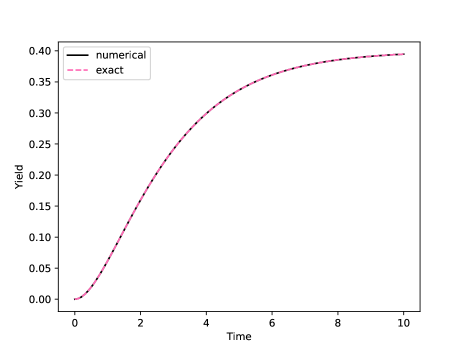
Figure 13: Comparing the numerical solution against the solutions found in equation (28).

Due to the length of the derivation, we confirm that our analysis is correct by comparing the numerical solution of the ODE to the exact solution we found in Figure 13. Finally, we look at interpolating between the two solutions; so given the solutions $y^{(1)}(t,B)$ and $y^{(2)}(t,B)$ corresponding to the linearization with stationary point in $S_{1}$ and $S_{2}$ respectively, we consider a solution of the form:

$$y(t,B|k_{1},k_{2},k_{3},\alpha)=(1-\mathcal{S}(B))y^{(1)}(t,B)+\mathcal{S}(B)y^{(2)}(t,B)$$ (29)

where $\mathcal{S}(x):=(1+e^{-\alpha_{sig}(x-0.5)})^{-1}$ is a sigmoid function centered at $B=0.5$ and where we have introduced a new hyper-parameter $\alpha_{sig}$. Finally, given Eq. (29) we can obtain the kernel. In particular, we want (29) to be a feature we are predicting on; therefore the kernel is simply the (dot) product of the features therefore:

$$k_{ode}((t,B),(t^{\prime},B^{\prime}))=y(t,B|k_{1},k_{2},k_{3},\alpha)\times y(t^{\prime},B^{\prime}|k_{1},k_{2},k_{3},\alpha)$$

And because we know we are simply approximating the data we can simply correct the model by adding an Gaussian Process correction; giving us the final kernel:

$$k_{joint}((t,B),(t^{\prime},B^{\prime}))=\alpha_{ode}k_{ode}((t,B),(t^{\prime},B^{\prime}))+\alpha_{rbf}k_{rbf}((t,B),(t^{\prime},B^{\prime}))$$

where $\alpha_{ode}$ and $\alpha_{rbf}$ are parameters we can learn, e.g. using the marginal likelihood.

References

- Audibert & Bubeck (2010) Audibert, J.-Y. and Bubeck, S. Best arm identification in multi-armed bandits. In Conference on Learning Theory, pp. 13–p, 2010.
- Besginow & Lange-Hegermann (2022) Besginow, A. and Lange-Hegermann, M. Constraining Gaussian processes to systems of linear ordinary differential equations. Advances in Neural Information Processing Systems, 35:29386–29399, 2022.
- Bogunovic et al. (2016) Bogunovic, I., Scarlett, J., Krause, A., and Cevher, V. Truncated variance reduction: A unified approach to Bayesian optimization and level-set estimation. Advances in Neural Information Processing Systems, 29, 2016.
- Boyd & Vandenberghe (2004) Boyd, S. and Vandenberghe, L. Convex optimization. Cambridge university press, 2004.
- Brennan et al. (2022) Brennan, J., Jain, L., Garman, S., Donnelly, A. E., Wright, E. S., and Jamieson, K. Sample-efficient identification of high-dimensional antibiotic synergy with a normalized diagonal sampling design. PLOS Computational Biology, 18(7):e1010311, 2022.
- Chaloner & Verdinelli (1995) Chaloner, K. and Verdinelli, I. Bayesian Experimental Design: A Review. Statist. Sci., 10(3):273–304, 08 1995.
- Che et al. (2023) Che, E., Wang, J., and Namkoong, H. Planning contextual adaptive experiments with model predictive control. NeurIPS 2023 Workshop on Adaptive Experimental Design and Active Learning in the Real World, 2023.
- Cheon et al. (2022) Cheon, M., Byun, H., and Lee, J. H. Reinforcement learning based multi-step look-ahead bayesian optimization. IFAC-PapersOnLine, 55(7):100–105, 2022.
- Cucker & Smale (2002) Cucker, F. and Smale, S. On the mathematical foundations of learning. Bulletin of the American mathematical society, 39(1):1–49, 2002.
- Felton et al. (2021) Felton, K., Rittig, J., and Lapkin, A. Summit: Benchmarking Machine Learning Methods for Reaction Optimisation. Chemistry Methods, February 2021.
- Fiez et al. (2019) Fiez, T., Jain, L., Jamieson, K. G., and Ratliff, L. Sequential experimental design for transductive linear bandits. Advances in neural information processing systems, 32, 2019.
- Folch et al. (2022) Folch, J. P., Zhang, S., Lee, R., Shafei, B., Walz, D., Tsay, C., van der Wilk, M., and Misener, R. SnAKe: Bayesian optimization with pathwise exploration. In Advances in Neural Information Processing Systems, volume 35, pp. 35226–35239, 2022.
- Folch et al. (2023a) Folch, J. P., Lee, R. M., Shafei, B., Walz, D., Tsay, C., van der Wilk, M., and Misener, R. Combining multi-fidelity modelling and asynchronous batch Bayesian optimization. Computers & Chemical Engineering, 172:108194, 2023a.
- Folch et al. (2023b) Folch, J. P., Odgers, J., Zhang, S., Lee, R. M., Shafei, B., Walz, D., Tsay, C., van der Wilk, M., and Misener, R. Practical path-based Bayesian optimization. NeurIPS 2023 Workshop on Adaptive Experimental Design and Active Learning in the Real World, 2023b.
- García et al. (1989) García, C. E., Prett, D. M., and Morari, M. Model predictive control: Theory and practice—A survey. Automatica, 25(3):335–348, 1989.
- Ginsbourger & Le Riche (2010) Ginsbourger, D. and Le Riche, R. Towards Gaussian process-based optimization with finite time horizon. In Advances in Model-Oriented Design and Analysis: Proceedings of the 9th International Workshop in Model-Oriented Design and Analysis, pp. 89–96. Springer, 2010.
- Gotovos et al. (2013) Gotovos, A., Casati, N., Hitz, G., and Krause, A. Active learning for level set estimation. In IJCAI 2013, 2013.
- Hazan et al. (2019) Hazan, E., Kakade, S., Singh, K., and Van Soest, A. Provably efficient maximum entropy exploration. In International Conference on Machine Learning, pp. 2681–2691. PMLR, 2019.
- Hennig & Schuler (2012) Hennig, P. and Schuler, C. J. Entropy search for information-efficient global optimization. Journal of Machine Learning Research, 13(6), 2012.
- Hernández-Lobato et al. (2014) Hernández-Lobato, J. M., Hoffman, M. W., and Ghahramani, Z. Predictive entropy search for efficient global optimization of black-box functions. Advances in neural information processing systems, 27, 2014.
- Hitz et al. (2014) Hitz, G., Gotovos, A., Garneau, M.-É., Pradalier, C., Krause, A., Siegwart, R. Y., et al. Fully autonomous focused exploration for robotic environmental monitoring. In 2014 IEEE International Conference on Robotics and Automation (ICRA), pp. 2658–2664. IEEE, 2014.
- Hutter et al. (2019) Hutter, F., Kotthoff, L., and Vanschoren, J. (eds.). Automated Machine Learning - Methods, Systems, Challenges. Springer, 2019.
- Hvarfner et al. (2022) Hvarfner, C., Hutter, F., and Nardi, L. Joint entropy search for maximally-informed Bayesian optimization. Advances in Neural Information Processing Systems, 35:11494–11506, 2022.
- Jaggi (2013) Jaggi, M. Revisiting Frank-Wolfe: Projection-Free Sparse Convex Optimization. In Dasgupta, S. and McAllester, D. (eds.), Proceedings of the 30th International Conference on Machine Learning, volume 28, pp. 427–435. PMLR, 17–19 Jun 2013.
- Jiang et al. (2020) Jiang, S., Chai, H., Gonzalez, J., and Garnett, R. Binoculars for efficient, nonmyopic sequential experimental design. In International Conference on Machine Learning, pp. 4794–4803. PMLR, 2020.
- Jones et al. (1998) Jones, D. R., Schonlau, M., and Welch, W. J. Efficient global optimization of expensive black-box functions. Journal of Global Optimization, 13(4):455–492, 1998.
- Kandasamy et al. (2018) Kandasamy, K., Krishnamurthy, A., Schneider, J., and Póczos, B. Parallelised Bayesian optimisation via Thompson sampling. In International Conference on Artificial Intelligence and Statistics, pp. 133–142. PMLR, 2018.
- Kirschner & Krause (2018) Kirschner, J. and Krause, A. Information directed sampling and bandits with heteroscedastic noise. In Conference On Learning Theory, pp. 358–384. PMLR, 2018.
- Kirschner et al. (2022) Kirschner, J., Mutný, M., Krause, A., Coello de Portugal, J., Hiller, N., and Snuverink, J. Tuning particle accelerators with safety constraints using Bayesian optimization. Phys. Rev. Accel. Beams, 25:062802, 2022.
- Lam et al. (2016) Lam, R., Willcox, K., and Wolpert, D. H. Bayesian optimization with a finite budget: An approximate dynamic programming approach. Advances in Neural Information Processing Systems, 29, 2016.
- Lee et al. (2021) Lee, E. H., Eriksson, D., Perrone, V., and Seeger, M. A nonmyopic approach to cost-constrained Bayesian optimization. In Uncertainty in Artificial Intelligence, pp. 568–577. PMLR, 2021.
- Marco et al. (2017) Marco, A., Berkenkamp, F., Hennig, P., Schoellig, A. P., Krause, A., Schaal, S., and Trimpe, S. Virtual vs. real: Trading off simulations and physical experiments in reinforcement learning with Bayesian optimization. In 2017 IEEE International Conference on Robotics and Automation (ICRA), pp. 1557–1563. IEEE, 2017.
- Mishra et al. (2023) Mishra, V., Astudillo, R., Frazier, P. I., and Zhang, F. Provably-convergent Bayesian source seeking with mobile agents in multimodal fields. In NeurIPS 2023 Workshop on Adaptive Experimental Design and Active Learning in the Real World, 2023.
- Mozharov et al. (2011) Mozharov, S., Nordon, A., Littlejohn, D., Wiles, C., Watts, P., Dallin, P., and Girkin, J. M. Improved method for kinetic studies in microreactors using flow manipulation and noninvasive Raman spectrometry. Journal of the American Chemical Society, 133(10):3601–3608, 2011.
- Mutny & Krause (2018) Mutny, M. and Krause, A. Efficient high dimensional Bayesian optimization with additivity and quadrature fourier features. Advances in Neural Information Processing Systems, 31, 2018.
- Mutny & Krause (2022) Mutny, M. and Krause, A. Experimental design for linear functionals in reproducing kernel Hilbert spaces. Advances in Neural Information Processing Systems, 35:20175–20188, 2022.
- Mutný et al. (2020) Mutný, M., Kirschner, J., and Krause, A. Experimental design for optimization of orthogonal projection pursuit models. In Proceedings of the 34th AAAI Conference on Artificial Intelligence (AAAI), 2020.
- Mutny et al. (2023) Mutny, M., Janik, T., and Krause, A. Active Exploration via Experiment Design in Markov Chains. In Proceedings of The 26th International Conference on Artificial Intelligence and Statistics, volume 206, pp. 7349–7374, 2023.
- Osborne et al. (2009) Osborne, M. A., Garnett, R., and Roberts, S. J. Gaussian processes for global optimization. 3rd International Conference on Learning and Intelligent Optimization (LION3), pp. 1–15, 2009.
- Paulson et al. (2022) Paulson, J. A., Sorouifar, F., and Chakrabarty, A. Efficient multi-step lookahead Bayesian optimization with local search constraints. In 2022 IEEE 61st Conference on Decision and Control (CDC), pp. 123–129. IEEE, 2022.
- Paulson et al. (2023) Paulson, J. A., Sorouifar, F., Laughman, C. R., and Chakrabarty, A. LSR-BO: Local search region constrained Bayesian optimization for performance optimization of vapor compression systems. In 2023 American Control Conference (ACC), pp. 576–582. IEEE, 2023.
- Pukelsheim (2006) Pukelsheim, F. Optimal Design of Experiments (Classics in Applied Mathematics) (Classics in Applied Mathematics, 50). Society for Industrial and Applied Mathematics, Philadelphia, PA, USA, 2006. ISBN 0898716047.
- Puterman (2014) Puterman, M. L. Markov decision processes: discrete stochastic dynamic programming. John Wiley Sons, 2014.
- Rahimi & Recht (2007) Rahimi, A. and Recht, B. Random features for large-scale kernel machines. Advances in neural information processing systems, 20, 2007.
- Ramesh et al. (2022) Ramesh, S. S., Sessa, P. G., Krause, A., and Bogunovic, I. Movement penalized Bayesian optimization with application to wind energy systems. In Advances in Neural Information Processing Systems, volume 35, pp. 27036–27048, 2022.
- Rasmussen & Williams (2005) Rasmussen, C. E. and Williams, C. K. I. Gaussian Processes for Machine Learning (Adaptive Computation and Machine Learning). The MIT Press, 2005.
- Samaniego et al. (2021) Samaniego, F. P., Reina, D. G., Marín, S. L. T., Arzamendia, M., and Gregor, D. O. A Bayesian optimization approach for water resources monitoring through an autonomous surface vehicle: The Ypacarai lake case study. IEEE Access, 9:9163–9179, 2021.
- Schrecker et al. (2023) Schrecker, L., Dickhaut, J., Holtze, C., Staehle, P., Vranceanu, M., Hellgardt, K., and Hii, K. K. M. Discovery of unexpectedly complex reaction pathways for the Knorr pyrazole synthesis via transient flow. Reaction Chemistry & Engineering, 8(1):41–46, 2023.
- Shahriari et al. (2016) Shahriari, B., Swersky, K., Wang, Z., Adams, R. P., and de Freitas, N. Taking the human out of the loop: A review of Bayesian optimization. Proceedings of the IEEE, 104(1):148–175, 2016.
- Soare et al. (2014) Soare, M., Lazaric, A., and Munos, R. Best-arm identification in linear bandits. Advances in Neural Information Processing Systems, 27, 2014.
- Srinivas et al. (2009) Srinivas, N., Krause, A., Kakade, S. M., and Seeger, M. Gaussian process optimization in the bandit setting: No regret and experimental design. arXiv preprint arXiv:0912.3995, 2009.
- Sullivan et al. (2023) Sullivan, M., Gebbie, J., and Lipor, J. Adaptive sampling for seabed identification from ambient acoustic noise. IEEE CAMSAP, 2023.
- Tu et al. (2022) Tu, B., Gandy, A., Kantas, N., and Shafei, B. Joint entropy search for multi-objective Bayesian optimization. Advances in Neural Information Processing Systems, 35:9922–9938, 2022.
- Vellanki et al. (2017) Vellanki, P., Rana, S., Gupta, S., Rubin, D., Sutti, A., Dorin, T., Height, M., Sanders, P., and Venkatesh, S. Process-constrained batch Bayesian optimisation. In Advances in Neural Information Processing Systems. Curran Associates, Inc., 2017.
- Wang & Jegelka (2017) Wang, Z. and Jegelka, S. Max-value entropy search for efficient Bayesian optimization. In International Conference on Machine Learning, pp. 3627–3635. PMLR, 2017.
- Williams & Seeger (2000) Williams, C. and Seeger, M. Using the Nyström method to speed up kernel machines. Advances in neural information processing systems, 13, 2000.
- Yang et al. (2023) Yang, A. X., Aitchison, L., and Moss, H. B. MONGOOSE: Path-wise smooth Bayesian optimisation via meta-learning. arXiv preprint arXiv:2302.11533, 2023.
- Yang et al. (2012) Yang, T., Li, Y.-F., Mahdavi, M., Jin, R., and Zhou, Z.-H. Nyström method vs random Fourier features: A theoretical and empirical comparison. Advances in neural information processing systems, 25, 2012.
- Yu et al. (2006) Yu, K., Bi, J., and Tresp, V. Active learning via transductive experimental design. In Proceedings of the 23rd international conference on Machine learning, pp. 1081–1088, 2006.