Asymptotic Weak Gravity Conjecture in
M-theory on $K3\times K3$

Abstract

The Asymptotic WGC has been proposed as a special case of the tower WGC that probes infinite distances in the moduli space corresponding to weakly coupled gauge regimes. The conjecture has been studied in M-theory on Calabi-Yau threefold (CY3) with finite volume inducing a 5D effective QFT. In this paper, we extend the scope of the previous study to encompass lower dimensions, particularly we generalise the obtained 5D asymptotic WGC to the effective field theory (EFT_3D) coupled to 3D gravity that descends from M-theory compactified on Calabi-Yau fourfold with an emphasis on $K3\times K3$.  We find that the CY4 has three fibration structures labelled as line Type-$\mathbb{T}^{2}$, surface Type-$\mathbb{S}$ and bulk Type-$\mathbb{V}$. The emergent EFT_3D is shown to have 2+2 towers of particles states termed as the BPS $\mathcal{T}_{M_{\mathrm{k}}\rightarrow 0}^{\text{{bps}}}$ and $\mathcal{T}_{M_{\mathrm{k}}\rightarrow\infty}^{\text{{bps}}}$ as well as the non-BPS $\mathcal{T}_{M_{\mathrm{k}}\rightarrow 0}^{\text{{n-bps}}}$ and $\mathcal{T}_{M_{\mathrm{k}}\rightarrow\infty}^{\text{{n-bps}}}$. To ensure the viability of the 3D Asymptotic WGC, we give explicit calculations to thoroughly test the swampland constraint for both the weakly and strongly gauge coupled regimes. Additional aspects, including the gauge symmetry breaking and duality symmetry are also investigated.

1 Introduction

Indubitably, the Swampland Program represents one of the major leaps and breakthroughs in our comprehension of quantum gravity 1 -3C . It provides a protocol to filter the effective field theories admitting a UV completion based on a set of consistency constraints known as Swampland Conjectures. Among the inaugural Swampland criteria, we cite (i) the Weak Gravity Conjecture (WGC) 4A -8 expecting the presence of at least one super-extremal particle. One of its most potent refinements is (ii) the so-called Tower WGC predicting the existence of a tower of massive charged states satisfying the WGC 9A , instead of the lone super-extremal particle required by the mild version; and (iii) the Swampland Distance conjecture (SDC) stipulating the emergence of an infinite tower of states that becomes asymptotically massless at large distances in the moduli space 10 -11B .

Using principles of the tower WGC and SDC, a new version of the WGC was obtained in 12 following an investigation of the aforementioned conjectures in M- theory on Calabi-Yau threefold (CY3) with a weak coupling regime 11A ; 12 ; it is labeled the Asymptotic-WGC. In fact, to study the resulting 5D effective field theory ($\emph{EFT}_{5D}$) in the infinite distance limit, while gravity remains dynamical, one would require that the volume $\mathcal{V}_{CY_{3}}$ of the internal complex threefold stay finite ($\mathcal{V}_{CY_{3}}<\infty$). This condition on the volume imposes a certain structure on the CY3 fibration: $\mathcal{F}_{fiber}\times\mathbb{B}_{base}$, to be $(1)$ either of a line fiber of Type-$\mathbb{T}^{2}$; or $(2)$ a surface fiber of Type-K3 or Type-$\mathbb{T}^{4}$. For these three Type-forms, the volume of the fiber $\mathcal{F}_{fiber}$ shrinks to zero in the infinite distance limit of the Kahler moduli space of the EFT_5D; while the volume of the base $\mathbb{B}_{base}$ expands to infinity in such a way that the full volume $\mathcal{V}_{CY_{3}}$ of the CY3, naively given by $\mathcal{V}_{\mathcal{F}_{fiber}}\times\mathcal{V}_{\mathbb{B}_{base}},$ remains finite.

The effective gauge theory coupled to gravity (which is now dynamical by taking a finite CY volume) has (i) a weak gauge coupling regime in the large distance limit ($g_{YM}\rightarrow 0$); and (ii) a charge lattice $\mathfrak{Q}$ endowed by rays (charge directions) hosting towers of BPS and non-BPS states satisfying the WGC 12 . From this perspective, the Asymptotic WGC can be seen as a special case of the Tower WGC in the sense that it only involves a particular region of the moduli space (i.e weakly coupled directions of the charge lattice); whereas the Tower WGC expects towers of states in all directions independently of the weak coupling limits. The weak gauge coupling regime is particularly interesting because it supplies properties that are not allowed otherwise; such as the relation between the extremality bound and the Repulsive Force Conjecture 13 as well as the precise calculation of the charge to mass ratio of non-BPS particle states 12 .

Furthermore, successful tests of the asymptotic WGC have been realized in both F-theory on elliptically fibered Calabi-Yau fourfolds 14A and M-theory on Calabi-Yau threefolds 12 . In the latter, the infinite distance limit fixes the fibration structure to two Type-forms: either Type-$\mathbb{T}^{2}$ or Type-$K3$/$\mathbb{T}^{4}$. Therein, some directions of the EFT_5D’s charge lattice hold the condition of the weak gauge coupling regime formulated as12 ; 14A :

$$\frac{\Lambda_{\text{{wgc}}}^{2}}{\Lambda_{\text{{qg}}}^{2}}\qquad\rightarrow\qquad 0$$ (1)

where $\Lambda_{\text{{wgc}}}$ is the magnetic WGC scale of the EFT${}_{5D},$ and $\Lambda_{\text{{qg}}}$ is the species scale; i.e the scale above which quantum gravity becomes strongly coupled instigating therefore a change of its dynamics 14B ; 14C . The above condition indicates the presence of weakly coupled gauge groups along particular directions in the charge lattice of the effective theory. In the context of EFT${}_{5D},$ two types of towers of states were shown to satisfy the conjecture, given by BPS and non-BPS states. Other studies has focused solely on BPS states since the BPS bound aligns with the super-extremality bound, as well as the relation between their charge and mass fixed by supersymmetry 14D -14F .

In this paper, we investigate the Asymptotic WGC at infinite distance limit of the 3D effective field theory ($\emph{EFT}_{3D}$) coupled to 3D gravity. This effective gauge theory descends from M-theory compactified on Calabi-Yau fourfold (CY4=$X_{4}$) with finite volume ($\mathcal{V}_{CY_{4}}<\infty$) following the framework of the 5D EFT of 11A and 12 . Note however that most studies in the context of 3D gravity has focused on AdS theories 14G ; 6 particularly a study of the basic and tower WGC conjectures in 3D from the perspective of infrared consistency was performed in 9A ; 9B .

To probe the Asymptotic WGC in EFT_3D emerging from the compactification of M-theory on a Calabi-Yau fourfold, we begin by outlining the classification of the fibral structure of the CY4 in the infinite distance limit. We find three Type-forms labeled as the line Type-$\mathbb{T}^{2}$, the surface Type-$\mathbb{S}$ and the bulk Type-$\mathbb{V}$. The two first Type-forms are common with the $CY3$ fibral classification 11A ; infinite distance limits of CY3 has also been studied in 15 ; 16 . The new bulk Type- $\mathbb{V}$ is due to the higher dimension of CY4 compared to CY3. This classification will allow us to keep working in a regime where gravity is dynamical, by taking the volume $\mathcal{V}_{CY_{4}}$ finite in the infinite distance limit, while the fiber $\mathcal{F}_{fiber}$ of $X_{4}$ shrinks to zero and its base $\mathbb{B}_{base}$ expands to infinity.

Given the richness of the fibration structure of the Calabi-Yau manifold, it would be more informative to focus on the surface Type-$\mathbb{S}$ for the following reasons: First, the fibral surface $S_{\perp}$ and the base surface $S_{\parallel}$ have the mid- dimension of $X_{4}$. Second, this surface Type-$\mathbb{S}$ permits the implementation of discrete symmetries like the $\mathbb{Z}_{2}$ automorphism generated by the transposition $S_{\perp}\longleftrightarrow$ $S_{\parallel}$ leaving the Calabi-Yau fourfold invariant. In particular in 12 only the base was allowed to expand while the fiber shrinks for the purpose of providing a weak gauge coupling regime; for our 3D investigation, we will take advantage of the automorphism $S_{\perp}\longleftrightarrow$ $S_{\parallel}$ to go even further and allow both of them to expand or shrink as long as the total volume remains finite. This property will generate the discrete symmetry predicting the existence of two asymptotic limits of the WGC related by $\mathbb{Z}_{2}$-symmetry: the usual asymptotic WGC with weak gauge coupling investigated in 5D in addition to the asymptotic WGC derived in this paper predicting a dual strong gauge coupling regime. Even though we are primarily interested in the weak gauge coupling of the EFT_3D in the infinite distance limit, we show that in the Type-$\mathbb{S}$ fibration of $X_{4}$ with $\mathbb{S}$ taken as the K3 surface, both strong and weak regimes arise as the gauge symmetry breaks into weakly and strongly coupled gauge groups.

As for the towers of quantum states required by the conjecture, we show that the particles of the EFT_3D generate four series given by: $(\mathbf{i})$ A tower $\mathcal{T}_{M_{\mathrm{k}}\rightarrow 0}^{\text{{bps}}}$ of charged BPS particles with light masses that vanish in the infinite distance limit ($M_{\mathrm{k}}$ $\rightarrow 0$); it is labelled by the integer k. $(\mathbf{ii})$ A tower $\mathcal{T}_{M_{\mathrm{k}}\rightarrow\infty}^{\text{{bps}}}$ of charged BPS particles with extremely heavy masses ($M_{\mathrm{k}}\rightarrow\infty$). $(\mathbf{iii})$ A tower $\mathcal{T}_{M_{\mathrm{k}}\rightarrow 0}^{\text{{n-bps}}}$ of non-BPS particles having light masses. $(\mathbf{iv})$ A tower$\mathcal{T}_{M_{\mathrm{k}}\rightarrow\infty}^{\text{{n-bps}}}$ of non BPS particles with extremely heavy masses. These $2+2$ towers of particle states are related amongst others by the $\mathbb{Z}_{2}$ automorphism symmetry of the $\mathbb{S}_{\perp}\times$ $\mathbb{S}_{\parallel}$ fibration and the Weak/Strong gauge symmetry duality of the 3D effective gauge theory. More precisely we use the $\mathbb{Z}_{2}$ duality between weak and strong coupling limits to argue that in the strongly coupled regions in the moduli space of the EFT_3D, we can also expect the presence of super-extremal states, since these regions can be seen as weakly coupled in a dual frame. In consequence, the asymptotic WGC is supported by even more towers of states than previously anticipated, which is in line with the tower WGC.

To sum up, these are the major results of this current investigation:

(1)

We classify the possible fibrations of the Calabi-Yau fourfold in the infinite distance limit while maintaining a finite volume inducing an EFT_3D coupled to 3D gravity. We show that the $X_{4}$ has three different fibral structures labelled as Line Type-$\mathbb{T}^{2}$, Surface Type-$\mathbb{S}$, and Bulk Type-$\mathbb{V}$. This classification generalises the one obtained in 11A for the EFT_5D coupled to 5D gravity induced by M-theory on CY3 in the infinite distance limit.

(2)

Considering the Type-$\mathbb{S}$ structure of the Calabi-Yau fourfold namely $X_{4}$ $=$ $\mathbb{S}_{\perp}\times$ $\mathbb{S}_{\parallel}$ with an emphasis on the case $K3_{\perp}\times K3_{\parallel}$ , we generate a $\mathbb{Z}_{2}$- automorphism symmetry by allowing both the fiber and the base to either shrink or expand, provided that the overall volume is finite. This discrete symmetry is given by the transposition $K3_{\perp}\longleftrightarrow K3_{\parallel}$ including the permutation of their p-cycles. By taking advantage of the special properties of K3, we work out the two asymptotic gauge regimes (weak and strong) of the EFT_3D that are compatible with the tower WGC. We also give two claims (I and II) regarding the two gauge regimes of Asymptotic WGC that exhibit the Weak/Strong duality of this 3D effective gauge theory.

(3)

Using the wrapping of M2 and M5 branes on K3 cycles as well as the duality links with heterotic string 12 , we construct the content of the four aforementioned towers namely: the content of the $\mathcal{T}_{M_{\mathrm{k}}\rightarrow 0}^{\text{{bps}}}$ having light BPS particles. The $\mathcal{T}_{M_{\mathrm{k}}\rightarrow\infty}^{\text{{bps}}}$ having extremely heavy BPS particles. The content of $\mathcal{T}_{M_{\mathrm{k}}\rightarrow 0}^{\text{{n-bps}}}$ with light non-BPS particles. And the $\mathcal{T}_{M_{\mathrm{k}}\rightarrow\infty}^{\text{{n-bps}}}$ made of extremely heavy non BPS particles. These light and the heavy towers are related by the Weak/Strong gauge symmetry duality.

(4)

Using the link between asymptotic WGC and the Repulsive Force Conjecture (RFC) 13 , we give explicit verifications of the Asymptotic WGC for both weakly gauge coupled and strongly gauge coupled regimes in the EFT_3D. We perform this test first for the towers $\mathcal{T}_{M_{\mathrm{k}}\rightarrow 0}^{\text{{bps}}}$ and $\mathcal{T}_{M_{\mathrm{k}}\rightarrow\infty}^{\text{{bps}}}$ made of BPS particle states, then for $\mathcal{T}_{M_{\mathrm{k}}\rightarrow 0}^{\text{{n-bps}}}$ and $\mathcal{T}_{M_{\mathrm{k}}\rightarrow\infty}^{\text{{n-bps}}}$ made of non-BPS particle states. And because classical massless 3D gravity is topological, we forfeit the classical effects for a non trivial negative contribution ${{}\mathchoice{\mbox{\boldmath$\displaystyle\mathchar 291\relax$}}{\mbox{\boldmath$\textstyle\mathchar 291\relax$}}{\mbox{\boldmath$\scriptstyle\mathchar 291\relax$}}{\mbox{\boldmath$\scriptscriptstyle\mathchar 291\relax$}}}_{QG}$ originating from quantum corrections.

The organisation of this paper is as follows: In section 2, we generalize the results of 11A regarding EFT_5D, induced by $X_{3}$ in the infinite distance limit, towards EFT_3D descending from M-theory on Calabi-Yau fourfold $X_{4}$ with finite volume. In section 3, we investigate the physical implications of the geometry probed by M-theory on CY4 in the moduli space of the 3D effective theory. We give results on the gauge coupling regimes in the EFT_3D with $X_{4}=K3\times K3$. In section 4, we distinguish the different gauge regimes before constructing the four towers of particle states in EFT_3D candidates to satisfy the asymptotic WGC. In section 5, we give explicit calculations testing the Asymptotic WGC for both weak and strong regime. Last section is devoted to conclusions. In Appendix A we report some technical details on the underlying properties of the towers of BPS and non-BPS states.

2 Classification of fibers of CY4

In this section, we give first results on the large distance limit for M-theory on Calabi-Yau fourfold (CY4) with finite volume ($\mathcal{V}_{{\small CY}_{4}}<\infty).$ These results will be used later on for compactified M-theory with background

$$\mathcal{M}_{11D}=X_{4}\times\mathcal{M}_{3D}\qquad;\qquad X_{4}:=CY_{4}$$ (2)

where the compact $X_{4}$ is fibered like $\mathcal{F}_{n}\times\mathbb{B}_{4-n}$ with complex fiber dimension taking the three values $n=1,2,3.$ These results will be also used in the study of the Asymptotic Weak Gravity Conjecture (Asymptotic-WGC) in 3D space-time. To do so, we need two main properties.

$(\mathbf{A})$

being particularly interested in theories coupled to 3D (topological) gravity, we need to keep the volume of the complex 4d internal manifold $X_{4}$ finite

$$\mathcal{V}_{{\small CY}_{4}}:=\left(l_{11d}\right)^{8}\mathcal{V}_{{\small X}_{{\small 4}}}<\infty$$ (3)

where $l_{11d}=1/M_{11d}$ is the usual 11D fundamental length scale of M-theory 17A . Notice that the $\mathcal{V}_{{\small X}_{{\small 4}}}$ is dimensionless ($\left[\mathcal{V}_{{\small X}_{{\small 4}}}\right]=length^{0}$); and is related to the Planck mass $M_{\mathrm{Pl}}$ in three dimensions and the 11D mass scale via $4{{}\mathchoice{\mbox{\boldmath$\displaystyle\mathchar 281\relax$}}{\mbox{\boldmath$\textstyle\mathchar 281\relax$}}{\mbox{\boldmath$\scriptstyle\mathchar 281\relax$}}{\mbox{\boldmath$\scriptscriptstyle\mathchar 281\relax$}}}\mathcal{V}_{{\small X}_{{\small 4}}}\simeq M_{Pl}/M_{11d};$ i.e:

$$M_{11d}=\frac{M_{Pl}}{4{{}\mathchoice{\mbox{\boldmath$\displaystyle\mathchar 281\relax$}}{\mbox{\boldmath$\textstyle\mathchar 281\relax$}}{\mbox{\boldmath$\scriptstyle\mathchar 281\relax$}}{\mbox{\boldmath$\scriptscriptstyle\mathchar 281\relax$}}}\mathcal{V}_{{\small X}_{{\small 4}}}}$$ (4)

$(\mathbf{B})$

Below, we will be interested in the infinite distance limit in the (gauge region of the) moduli space $\mathfrak{M}_{X_{4}}$ of the effective field theory (EFT_3D) descending from M-theory on $X_{4}$. In this limit, we will take the volume $\mathcal{V}_{\mathcal{F}_{n}}$ of the fiber to shrink to zero whereas the volume $\mathcal{V}_{\mathbb{B}_{4-n}}$ of base diverges; i.e:

$$\mathcal{V}_{\mathcal{F}_{n}}\rightarrow 0\qquad and\qquad\mathcal{V}_{\mathbb{B}_{4-n}}\rightarrow\infty$$ (5)

while their product $\mathcal{V}_{\mathcal{F}_{n}}\times\mathcal{V}_{\mathbb{B}_{4-n}}$ is finite.

Thus, we need to construct CY manifolds $X_{4}$ which obey both the two above properties: $\left(\mathbf{A}\right)$ and $\left(\mathbf{B}\right).$ And this is the main goal of the investigation given in this section. To that purpose, we revisit in subsection 2.1 useful results on EFT_5D given by M-theory on Calabi-Yau threefolds CY${}_{3}:=X_{3}$ 11A ; 12 . In subsection 2.2, we give our results on the fibration structure of the Calabi-Yau fourfold that induces our EFT_3D in infinite distance limit in the moduli space.
As a front matter, notice that, as for finite distances in the moduli space of EFT_(11-2d)D, one can also distinguish various possible fibrations $\mathcal{F}_{n}\times\mathbb{B}_{d-n}$ of complex d-dimensional $CY_{d}:=X_{d}$ in the infinite distance limit (${{}\mathchoice{\mbox{\boldmath$\displaystyle\mathchar 277\relax$}}{\mbox{\boldmath$\textstyle\mathchar 277\relax$}}{\mbox{\boldmath$\scriptstyle\mathchar 277\relax$}}{\mbox{\boldmath$\scriptscriptstyle\mathchar 277\relax$}}}\rightarrow\infty$). For the case $d=4$ we are particularly interested into here, we have the following typical fibrations

internal X₄ fiber $$\mathcal{F}_{n}$$  base

(6)

such that the first Chern class $c_{1}\left(\mathcal{F}_{n}\times\mathbb{B}_{4-n}\right)$ vanishes. Note also that a fibered Calabi-Yau manifold must have a fiber which is also Calabi-Yau 17B , this will limit tremendously the number of the possibilities, especially for $\mathcal{F}_{1}$ and $\mathcal{F}_{2}.$ On the other hand the possibilities of $\mathcal{F}_{3}$ are vastly larger 18 ; 19 .
To build the $\mathcal{F}_{n}$ fibers and the corresponding $\mathbb{B}_{4-n}$ bases that can be used in Asymptotic-WGC of EFT_3D, we borrow ideas from the classification of fiber structure of on Calabi-Yau threefolds $X_{3}$ 11A  reviewed below.

2.1 Classification of X₃ fibers in infinite distance limit

Following 11A , we distinguish two kinds of fibrations in M-theory on Calabi-Yau threefolds in the infinite distance limit with three possible fibers (namely $\mathbb{T}^{2},$ K3 and $\mathbb{T}^{4}$ ). Depending on the dimension of the fiber, we have either

$$\mathcal{F}_{1}$$ X₃

(7)

with $\mathcal{F}_{1}$ a complex curve ($\dim_{\mathbb{C}}\mathcal{F}_{1}=1$); or

$$\mathcal{F}_{2}$$ X₃

(8)

with $\mathcal{F}_{2}$ a complex surface ($\dim_{\mathbb{C}}\mathcal{F}_{2}=2$). The emerging fibers for $\mathcal{F}_{1}$ and $\mathcal{F}_{2}$ in the infinite distance limit, result from taking a finite volume $\mathcal{V}_{{\small X}_{{\small 3}}}$ in order for the 5D gravity to remain dynamical. We start by parameterizing the Kahler 2-form $J$ of the X₃ like $J=\sum_{{{}\mathchoice{\mbox{\boldmath$\displaystyle\mathchar 278\relax$}}{\mbox{\boldmath$\textstyle\mathchar 278\relax$}}{\mbox{\boldmath$\scriptstyle\mathchar 278\relax$}}{\mbox{\boldmath$\scriptscriptstyle\mathchar 278\relax$}}}=1}^{h_{{\small X}_{{\small 3}}}^{1,1}}{{}\mathchoice{\mbox{\boldmath$\displaystyle\mathchar 285\relax$}}{\mbox{\boldmath$\textstyle\mathchar 285\relax$}}{\mbox{\boldmath$\scriptstyle\mathchar 285\relax$}}{\mbox{\boldmath$\scriptscriptstyle\mathchar 285\relax$}}}^{{{}\mathchoice{\mbox{\boldmath$\displaystyle\mathchar 278\relax$}}{\mbox{\boldmath$\textstyle\mathchar 278\relax$}}{\mbox{\boldmath$\scriptstyle\mathchar 278\relax$}}{\mbox{\boldmath$\scriptscriptstyle\mathchar 278\relax$}}}}J_{{{}\mathchoice{\mbox{\boldmath$\displaystyle\mathchar 278\relax$}}{\mbox{\boldmath$\textstyle\mathchar 278\relax$}}{\mbox{\boldmath$\scriptstyle\mathchar 278\relax$}}{\mbox{\boldmath$\scriptscriptstyle\mathchar 278\relax$}}}}$; which for convenience we present simply as:

$$J={{}\mathchoice{\mbox{\boldmath$\displaystyle\mathchar 277\relax$}}{\mbox{\boldmath$\textstyle\mathchar 277\relax$}}{\mbox{\boldmath$\scriptstyle\mathchar 277\relax$}}{\mbox{\boldmath$\scriptscriptstyle\mathchar 277\relax$}}}{{}\mathchoice{\mbox{\boldmath$\displaystyle\mathchar 285\relax$}}{\mbox{\boldmath$\textstyle\mathchar 285\relax$}}{\mbox{\boldmath$\scriptstyle\mathchar 285\relax$}}{\mbox{\boldmath$\scriptscriptstyle\mathchar 285\relax$}}}^{0}J_{0}+\frac{1}{{{}\mathchoice{\mbox{\boldmath$\displaystyle\mathchar 277\relax$}}{\mbox{\boldmath$\textstyle\mathchar 277\relax$}}{\mbox{\boldmath$\scriptstyle\mathchar 277\relax$}}{\mbox{\boldmath$\scriptscriptstyle\mathchar 277\relax$}}}^{{{}\mathchoice{\mbox{\boldmath$\displaystyle\mathchar 267\relax$}}{\mbox{\boldmath$\textstyle\mathchar 267\relax$}}{\mbox{\boldmath$\scriptstyle\mathchar 267\relax$}}{\mbox{\boldmath$\scriptscriptstyle\mathchar 267\relax$}}}}}\sum_{i=1}^{\mathrm{r}}{{}\mathchoice{\mbox{\boldmath$\displaystyle\mathchar 285\relax$}}{\mbox{\boldmath$\textstyle\mathchar 285\relax$}}{\mbox{\boldmath$\scriptstyle\mathchar 285\relax$}}{\mbox{\boldmath$\scriptscriptstyle\mathchar 285\relax$}}}^{i}J_{i}$$ (9)

with $r=h_{{\small X}_{{\small 3}}}^{1,1}-1.$ In this expansion, the real $\textstyle\mathchar 277\relax$ is a spectral parameter characterizing the infinite distance limit in the moduli space of the theory; the infinite distance limit is implemented by the asymptotic limit ${{}\mathchoice{\mbox{\boldmath$\displaystyle\mathchar 277\relax$}}{\mbox{\boldmath$\textstyle\mathchar 277\relax$}}{\mbox{\boldmath$\scriptstyle\mathchar 277\relax$}}{\mbox{\boldmath$\scriptscriptstyle\mathchar 277\relax$}}}\rightarrow\infty$. The $J_{0}$ is a representative divisor in the base $\mathbb{B}_{2}$ (that can be imagined as the projective $\mathbb{P}^{2}$ or $\mathbb{P}^{1}\times\mathbb{P}^{1}$); the choice of one divisor is to simplify the calculations in solving the constraints $\left(\mathbf{A}\right)$ and $\left(\mathbf{B}\right)$. The other $J_{i}$’s in (9) concern the fiber $\mathcal{F}_{1}$. The real positive ${{}\mathchoice{\mbox{\boldmath$\displaystyle\mathchar 285\relax$}}{\mbox{\boldmath$\textstyle\mathchar 285\relax$}}{\mbox{\boldmath$\scriptstyle\mathchar 285\relax$}}{\mbox{\boldmath$\scriptscriptstyle\mathchar 285\relax$}}}^{0}$ and ${{}\mathchoice{\mbox{\boldmath$\displaystyle\mathchar 285\relax$}}{\mbox{\boldmath$\textstyle\mathchar 285\relax$}}{\mbox{\boldmath$\scriptstyle\mathchar 285\relax$}}{\mbox{\boldmath$\scriptscriptstyle\mathchar 285\relax$}}}^{i}$ parameters are the volumes of the dual 2-cycles in the homology $H_{2}(X_{3})$.

Using (9), the classification of 11A can be shortly presented in terms of the value of the monomials $J_{0}^{n};$ we have:

$\left(\mathbf{1}\right)$

Type-$\mathbb{T}^{2}$ form:
It corresponds to $J_{0}^{3}=0$ but $J_{0}^{2}\neq 0$ 21 ; 22 Here, the fiber $\mathcal{F}_{1}$ in the fibration (7) is given by a 2-torus $\mathbb{T}^{2}$ (elliptic curve $\mathcal{E}$).
The Kahler form is given by

$$J={{}\mathchoice{\mbox{\boldmath$\displaystyle\mathchar 277\relax$}}{\mbox{\boldmath$\textstyle\mathchar 277\relax$}}{\mbox{\boldmath$\scriptstyle\mathchar 277\relax$}}{\mbox{\boldmath$\scriptscriptstyle\mathchar 277\relax$}}}{{}\mathchoice{\mbox{\boldmath$\displaystyle\mathchar 285\relax$}}{\mbox{\boldmath$\textstyle\mathchar 285\relax$}}{\mbox{\boldmath$\scriptstyle\mathchar 285\relax$}}{\mbox{\boldmath$\scriptscriptstyle\mathchar 285\relax$}}}^{0}J_{0}+\frac{1}{{{}\mathchoice{\mbox{\boldmath$\displaystyle\mathchar 277\relax$}}{\mbox{\boldmath$\textstyle\mathchar 277\relax$}}{\mbox{\boldmath$\scriptstyle\mathchar 277\relax$}}{\mbox{\boldmath$\scriptscriptstyle\mathchar 277\relax$}}}^{2}}\sum_{i=1}^{\mathrm{r}}{{}\mathchoice{\mbox{\boldmath$\displaystyle\mathchar 285\relax$}}{\mbox{\boldmath$\textstyle\mathchar 285\relax$}}{\mbox{\boldmath$\scriptstyle\mathchar 285\relax$}}{\mbox{\boldmath$\scriptscriptstyle\mathchar 285\relax$}}}^{i}J_{i}$$ (10)

Using (10), it results that the volume $\mathcal{V}_{\mathcal{F}_{1}}$ of the fiber and the volume $\mathcal{V}_{\mathbb{B}_{2}}$ of the base behave like

$$\mathcal{V}_{\mathcal{F}_{1}}\sim\frac{1}{{{}\mathchoice{\mbox{\boldmath$\displaystyle\mathchar 277\relax$}}{\mbox{\boldmath$\textstyle\mathchar 277\relax$}}{\mbox{\boldmath$\scriptstyle\mathchar 277\relax$}}{\mbox{\boldmath$\scriptscriptstyle\mathchar 277\relax$}}}^{2}}T_{finite}\qquad,\qquad\mathcal{V}_{\mathbb{B}_{2}}\sim{{}\mathchoice{\mbox{\boldmath$\displaystyle\mathchar 277\relax$}}{\mbox{\boldmath$\textstyle\mathchar 277\relax$}}{\mbox{\boldmath$\scriptstyle\mathchar 277\relax$}}{\mbox{\boldmath$\scriptscriptstyle\mathchar 277\relax$}}}^{2}B_{finite}$$ (11)

where $T_{finite}$ and $B_{finite}$ take finite values in the limit ${{}\mathchoice{\mbox{\boldmath$\displaystyle\mathchar 277\relax$}}{\mbox{\boldmath$\textstyle\mathchar 277\relax$}}{\mbox{\boldmath$\scriptstyle\mathchar 277\relax$}}{\mbox{\boldmath$\scriptscriptstyle\mathchar 277\relax$}}}\rightarrow\infty$. Notice that while $\lim_{{{}\mathchoice{\mbox{\boldmath$\displaystyle\mathchar 277\relax$}}{\mbox{\boldmath$\textstyle\mathchar 277\relax$}}{\mbox{\boldmath$\scriptstyle\mathchar 277\relax$}}{\mbox{\boldmath$\scriptscriptstyle\mathchar 277\relax$}}}\rightarrow\infty}\mathcal{V}_{\mathcal{F}_{1}}=0$ and $\lim_{{{}\mathchoice{\mbox{\boldmath$\displaystyle\mathchar 277\relax$}}{\mbox{\boldmath$\textstyle\mathchar 277\relax$}}{\mbox{\boldmath$\scriptstyle\mathchar 277\relax$}}{\mbox{\boldmath$\scriptscriptstyle\mathchar 277\relax$}}}\rightarrow\infty}\mathcal{V}_{\mathbb{B}_{2}}=\infty$, the total volume of the $X_{3}$ remains finite even in the infinite distance limit where it takes the value

$$\lim_{{{}\mathchoice{\mbox{\boldmath$\displaystyle\mathchar 277\relax$}}{\mbox{\boldmath$\textstyle\mathchar 277\relax$}}{\mbox{\boldmath$\scriptstyle\mathchar 277\relax$}}{\mbox{\boldmath$\scriptscriptstyle\mathchar 277\relax$}}}\rightarrow\infty}\mathcal{V}_{{\small CY}_{{\small 3}}}\simeq T_{finite}\times B_{finite}$$ (12)

$\left(\mathbf{2}\right)$

Type-$\mathbb{S}$ forms:
It corresponds to $J_{0}^{3}=0$ and $J_{0}^{2}=0$ 23A . In this Type- surface form, the fiber $\mathcal{F}_{2}$ in the second structure in eq(8) is a complex surface which, in the infinite distance limit, has been shown to be $\left(\mathbf{a}\right)$ either a K3 surface; or $\left(\mathbf{b}\right)$ an abelian Schoen surface having the topology of $\mathbb{T}^{4}$.
For the generalization of this classification to the case of the $X_{4},$ it is interesting to think about the K3 and the $\mathbb{T}^{4}$ manifolds in terms of fibrations using the complex one dimensional lines $\mathbb{P}^{1}$ and $\mathbb{T}^{2}$. The two possible $\mathcal{F}_{2}\sim\mathbb{S}$ can be presented as follows:

$$\left(\mathbf{a}\right)$$ :

:

(13)

both of hem having $c_{1}\left(T\mathbb{S}\right)=0$; thus ruling out surfaces $\mathbb{S}$ like $\mathbb{P}^{1}\times\mathbb{P}^{1}.$
Notice that in both the Type-$\mathbb{S}$ forms (13), the Kahler form $J$ can be parameterised as

$$J={{}\mathchoice{\mbox{\boldmath$\displaystyle\mathchar 277\relax$}}{\mbox{\boldmath$\textstyle\mathchar 277\relax$}}{\mbox{\boldmath$\scriptstyle\mathchar 277\relax$}}{\mbox{\boldmath$\scriptscriptstyle\mathchar 277\relax$}}}{{}\mathchoice{\mbox{\boldmath$\displaystyle\mathchar 285\relax$}}{\mbox{\boldmath$\textstyle\mathchar 285\relax$}}{\mbox{\boldmath$\scriptstyle\mathchar 285\relax$}}{\mbox{\boldmath$\scriptscriptstyle\mathchar 285\relax$}}}^{0}J_{0}+\frac{1}{\sqrt{{{}\mathchoice{\mbox{\boldmath$\displaystyle\mathchar 277\relax$}}{\mbox{\boldmath$\textstyle\mathchar 277\relax$}}{\mbox{\boldmath$\scriptstyle\mathchar 277\relax$}}{\mbox{\boldmath$\scriptscriptstyle\mathchar 277\relax$}}}}}\sum_{i=1}^{\mathrm{r}}{{}\mathchoice{\mbox{\boldmath$\displaystyle\mathchar 285\relax$}}{\mbox{\boldmath$\textstyle\mathchar 285\relax$}}{\mbox{\boldmath$\scriptstyle\mathchar 285\relax$}}{\mbox{\boldmath$\scriptscriptstyle\mathchar 285\relax$}}}^{i}J_{i}$$ (14)

Using this expansion, the volume $\mathcal{F}_{2}$ of the fiber and the volume $\mathcal{V}_{\mathbb{B}_{1}}$ of the base behave like

$$\mathcal{V}_{\mathcal{F}_{2}}\sim\frac{1}{{{}\mathchoice{\mbox{\boldmath$\displaystyle\mathchar 277\relax$}}{\mbox{\boldmath$\textstyle\mathchar 277\relax$}}{\mbox{\boldmath$\scriptstyle\mathchar 277\relax$}}{\mbox{\boldmath$\scriptscriptstyle\mathchar 277\relax$}}}}T_{finite}^{\prime}\qquad,\qquad\mathcal{V}_{\mathbb{B}_{1}}\sim{{}\mathchoice{\mbox{\boldmath$\displaystyle\mathchar 277\relax$}}{\mbox{\boldmath$\textstyle\mathchar 277\relax$}}{\mbox{\boldmath$\scriptstyle\mathchar 277\relax$}}{\mbox{\boldmath$\scriptscriptstyle\mathchar 277\relax$}}}B_{finite}^{\prime}$$ (15)

where $T_{finite}^{\prime}$ and $B_{finite}^{\prime}$ take finite values in the limit ${{}\mathchoice{\mbox{\boldmath$\displaystyle\mathchar 277\relax$}}{\mbox{\boldmath$\textstyle\mathchar 277\relax$}}{\mbox{\boldmath$\scriptstyle\mathchar 277\relax$}}{\mbox{\boldmath$\scriptscriptstyle\mathchar 277\relax$}}}\rightarrow\infty$. Notice also that these two Type-$\mathbb{S}$ forms (13) are distinguished by the value of the second Chern class c${}_{2}\left(T\mathbb{S}\right)$ which is equal to 24 for K3 and vanishes for $\mathbb{T}^{4}$. Notice moreover that the full volume of the $X_{3}$ remains finite even in the infinite distance limit; we have

$$\lim_{{{}\mathchoice{\mbox{\boldmath$\displaystyle\mathchar 277\relax$}}{\mbox{\boldmath$\textstyle\mathchar 277\relax$}}{\mbox{\boldmath$\scriptstyle\mathchar 277\relax$}}{\mbox{\boldmath$\scriptscriptstyle\mathchar 277\relax$}}}\rightarrow\infty}\mathcal{V}_{{\small X}_{{\small 3}}}\simeq T_{finite}^{\prime}\times B_{finite}^{\prime}$$ (16)

2.2 Generalization to X₄ in the infinite distance limit

Mimicking the above description regarding the possible fibration forms of the Calabi-Yau threefold $X_{3}$ in the infinite distance limit, one can deduce straightforwardly the classification of the fibers of the manifolds (6) without going much into technical details.
The classification of the $\mathcal{F}_{n}$ in the fibration (6) at ${{}\mathchoice{\mbox{\boldmath$\displaystyle\mathchar 277\relax$}}{\mbox{\boldmath$\textstyle\mathchar 277\relax$}}{\mbox{\boldmath$\scriptstyle\mathchar 277\relax$}}{\mbox{\boldmath$\scriptscriptstyle\mathchar 277\relax$}}}\rightarrow\infty$ can be done according to the values of the monomial $J_{0}^{n}$. Extending the construction done for $X_{3}$ towards $X_{4}$; we end up with the following result:

$(\mathbf{A)}$

Type-$\mathbb{T}^{2}$ form of the X₄: 
It corresponds to the constraint relations

$$J_{0}^{4}=0\qquad,\qquad J_{0}^{3}\neq 0$$ (17)

In this case, the Kahler 2-form $J$ can be parameterized by as follows

$$J={{}\mathchoice{\mbox{\boldmath$\displaystyle\mathchar 277\relax$}}{\mbox{\boldmath$\textstyle\mathchar 277\relax$}}{\mbox{\boldmath$\scriptstyle\mathchar 277\relax$}}{\mbox{\boldmath$\scriptscriptstyle\mathchar 277\relax$}}}{{}\mathchoice{\mbox{\boldmath$\displaystyle\mathchar 285\relax$}}{\mbox{\boldmath$\textstyle\mathchar 285\relax$}}{\mbox{\boldmath$\scriptstyle\mathchar 285\relax$}}{\mbox{\boldmath$\scriptscriptstyle\mathchar 285\relax$}}}^{0}J_{0}+\frac{1}{{{}\mathchoice{\mbox{\boldmath$\displaystyle\mathchar 277\relax$}}{\mbox{\boldmath$\textstyle\mathchar 277\relax$}}{\mbox{\boldmath$\scriptstyle\mathchar 277\relax$}}{\mbox{\boldmath$\scriptscriptstyle\mathchar 277\relax$}}}^{3}}\sum_{i=1}^{\mathrm{r}}{{}\mathchoice{\mbox{\boldmath$\displaystyle\mathchar 285\relax$}}{\mbox{\boldmath$\textstyle\mathchar 285\relax$}}{\mbox{\boldmath$\scriptstyle\mathchar 285\relax$}}{\mbox{\boldmath$\scriptscriptstyle\mathchar 285\relax$}}}^{i}J_{i}$$ (18)

with $r=h^{1,1}(X_{4})-1.$ Expressing this expansion shortly as $J={{}\mathchoice{\mbox{\boldmath$\displaystyle\mathchar 277\relax$}}{\mbox{\boldmath$\textstyle\mathchar 277\relax$}}{\mbox{\boldmath$\scriptstyle\mathchar 277\relax$}}{\mbox{\boldmath$\scriptscriptstyle\mathchar 277\relax$}}}{{}\mathchoice{\mbox{\boldmath$\displaystyle\mathchar 285\relax$}}{\mbox{\boldmath$\textstyle\mathchar 285\relax$}}{\mbox{\boldmath$\scriptstyle\mathchar 285\relax$}}{\mbox{\boldmath$\scriptscriptstyle\mathchar 285\relax$}}}^{0}J_{0}+\frac{1}{{{}\mathchoice{\mbox{\boldmath$\displaystyle\mathchar 277\relax$}}{\mbox{\boldmath$\textstyle\mathchar 277\relax$}}{\mbox{\boldmath$\scriptstyle\mathchar 277\relax$}}{\mbox{\boldmath$\scriptscriptstyle\mathchar 277\relax$}}}^{3}}K$ with $K=\sum_{i=1}^{\mathrm{r}}{{}\mathchoice{\mbox{\boldmath$\displaystyle\mathchar 285\relax$}}{\mbox{\boldmath$\textstyle\mathchar 285\relax$}}{\mbox{\boldmath$\scriptstyle\mathchar 285\relax$}}{\mbox{\boldmath$\scriptscriptstyle\mathchar 285\relax$}}}^{i}J_{i}$ and using $J_{0}^{4}=0$ and $J_{0}^{3}\neq 0$, we have

$$J^{4}=\left(4{{}\mathchoice{\mbox{\boldmath$\displaystyle\mathchar 285\relax$}}{\mbox{\boldmath$\textstyle\mathchar 285\relax$}}{\mbox{\boldmath$\scriptstyle\mathchar 285\relax$}}{\mbox{\boldmath$\scriptscriptstyle\mathchar 285\relax$}}}_{0}^{3}\right)J_{0}^{3}K+\frac{6{{}\mathchoice{\mbox{\boldmath$\displaystyle\mathchar 285\relax$}}{\mbox{\boldmath$\textstyle\mathchar 285\relax$}}{\mbox{\boldmath$\scriptstyle\mathchar 285\relax$}}{\mbox{\boldmath$\scriptscriptstyle\mathchar 285\relax$}}}_{0}^{2}}{{{}\mathchoice{\mbox{\boldmath$\displaystyle\mathchar 277\relax$}}{\mbox{\boldmath$\textstyle\mathchar 277\relax$}}{\mbox{\boldmath$\scriptstyle\mathchar 277\relax$}}{\mbox{\boldmath$\scriptscriptstyle\mathchar 277\relax$}}}^{4}}J_{0}^{2}K^{2}+\frac{4{{}\mathchoice{\mbox{\boldmath$\displaystyle\mathchar 285\relax$}}{\mbox{\boldmath$\textstyle\mathchar 285\relax$}}{\mbox{\boldmath$\scriptstyle\mathchar 285\relax$}}{\mbox{\boldmath$\scriptscriptstyle\mathchar 285\relax$}}}^{0}}{{{}\mathchoice{\mbox{\boldmath$\displaystyle\mathchar 277\relax$}}{\mbox{\boldmath$\textstyle\mathchar 277\relax$}}{\mbox{\boldmath$\scriptstyle\mathchar 277\relax$}}{\mbox{\boldmath$\scriptscriptstyle\mathchar 277\relax$}}}^{8}}J_{0}K^{3}+\frac{1}{{{}\mathchoice{\mbox{\boldmath$\displaystyle\mathchar 277\relax$}}{\mbox{\boldmath$\textstyle\mathchar 277\relax$}}{\mbox{\boldmath$\scriptstyle\mathchar 277\relax$}}{\mbox{\boldmath$\scriptscriptstyle\mathchar 277\relax$}}}^{12}}K^{4}$$ (19)

behaving in powers of $1/{{}\mathchoice{\mbox{\boldmath$\displaystyle\mathchar 277\relax$}}{\mbox{\boldmath$\textstyle\mathchar 277\relax$}}{\mbox{\boldmath$\scriptstyle\mathchar 277\relax$}}{\mbox{\boldmath$\scriptscriptstyle\mathchar 277\relax$}}}$ as

$$J^{4}=\left(4{{}\mathchoice{\mbox{\boldmath$\displaystyle\mathchar 285\relax$}}{\mbox{\boldmath$\textstyle\mathchar 285\relax$}}{\mbox{\boldmath$\scriptstyle\mathchar 285\relax$}}{\mbox{\boldmath$\scriptscriptstyle\mathchar 285\relax$}}}_{0}^{3}\right)J_{0}^{3}K+\mathcal{O}\left(\frac{1}{{{}\mathchoice{\mbox{\boldmath$\displaystyle\mathchar 277\relax$}}{\mbox{\boldmath$\textstyle\mathchar 277\relax$}}{\mbox{\boldmath$\scriptstyle\mathchar 277\relax$}}{\mbox{\boldmath$\scriptscriptstyle\mathchar 277\relax$}}}^{4}}\right)$$ (20)

Here, the $\mathcal{F}_{1}$ in eq(6) is a complex line homotopic to $\mathbb{T}^{2};$ in a similar way as in the case of $X_{3}.$ In the infinite distance limit, the volume $\mathcal{V}_{\mathcal{F}_{1}}$ of the fiber $\mathcal{F}_{1}$ and the volume $\mathcal{V}_{\mathbb{B}_{3}}$ of the base $\mathbb{B}_{3}$ behave in terms of the spectral parameter $\textstyle\mathchar 277\relax$ like

$$\mathcal{V}_{\mathcal{F}_{1}}\sim\frac{1}{{{}\mathchoice{\mbox{\boldmath$\displaystyle\mathchar 277\relax$}}{\mbox{\boldmath$\textstyle\mathchar 277\relax$}}{\mbox{\boldmath$\scriptstyle\mathchar 277\relax$}}{\mbox{\boldmath$\scriptscriptstyle\mathchar 277\relax$}}}^{3}}\mathrm{{{}\mathchoice{\mbox{\boldmath$\displaystyle\mathchar 284\relax$}}{\mbox{\boldmath$\textstyle\mathchar 284\relax$}}{\mbox{\boldmath$\scriptstyle\mathchar 284\relax$}}{\mbox{\boldmath$\scriptscriptstyle\mathchar 284\relax$}}}}_{finite}\qquad,\qquad\mathcal{V}_{\mathbb{B}_{3}}\sim{{}\mathchoice{\mbox{\boldmath$\displaystyle\mathchar 277\relax$}}{\mbox{\boldmath$\textstyle\mathchar 277\relax$}}{\mbox{\boldmath$\scriptstyle\mathchar 277\relax$}}{\mbox{\boldmath$\scriptscriptstyle\mathchar 277\relax$}}}^{3}\mathrm{{{}\mathchoice{\mbox{\boldmath$\displaystyle\mathchar 268\relax$}}{\mbox{\boldmath$\textstyle\mathchar 268\relax$}}{\mbox{\boldmath$\scriptstyle\mathchar 268\relax$}}{\mbox{\boldmath$\scriptscriptstyle\mathchar 268\relax$}}}}_{finite}$$ (21)

where $\mathrm{{{}\mathchoice{\mbox{\boldmath$\displaystyle\mathchar 284\relax$}}{\mbox{\boldmath$\textstyle\mathchar 284\relax$}}{\mbox{\boldmath$\scriptstyle\mathchar 284\relax$}}{\mbox{\boldmath$\scriptscriptstyle\mathchar 284\relax$}}}}_{finite}$ and $\mathrm{{{}\mathchoice{\mbox{\boldmath$\displaystyle\mathchar 268\relax$}}{\mbox{\boldmath$\textstyle\mathchar 268\relax$}}{\mbox{\boldmath$\scriptstyle\mathchar 268\relax$}}{\mbox{\boldmath$\scriptscriptstyle\mathchar 268\relax$}}}}_{finite}$ are functions of $\textstyle\mathchar 277\relax$ taken finite everywhere in the moduli space $\mathfrak{M}_{{\small CY}_{{\small 4}}}$ of the 3D effective field theory. The volumes $\mathcal{V}_{\mathcal{F}_{1}}$ and $\mathcal{V}_{\mathbb{B}_{3}}$ have rapid singularities in the limit ${{}\mathchoice{\mbox{\boldmath$\displaystyle\mathchar 277\relax$}}{\mbox{\boldmath$\textstyle\mathchar 277\relax$}}{\mbox{\boldmath$\scriptstyle\mathchar 277\relax$}}{\mbox{\boldmath$\scriptscriptstyle\mathchar 277\relax$}}}\rightarrow\infty$ (shrinking $\mathcal{F}_{1}$ and diverging $\mathbb{B}_{3}$); but in such way that the full volume of the X₄ remains finite

$$\lim_{{{}\mathchoice{\mbox{\boldmath$\displaystyle\mathchar 277\relax$}}{\mbox{\boldmath$\textstyle\mathchar 277\relax$}}{\mbox{\boldmath$\scriptstyle\mathchar 277\relax$}}{\mbox{\boldmath$\scriptscriptstyle\mathchar 277\relax$}}}\rightarrow\infty}\mathcal{V}_{{\small X}_{{\small 4}}}\simeq\mathrm{{{}\mathchoice{\mbox{\boldmath$\displaystyle\mathchar 284\relax$}}{\mbox{\boldmath$\textstyle\mathchar 284\relax$}}{\mbox{\boldmath$\scriptstyle\mathchar 284\relax$}}{\mbox{\boldmath$\scriptscriptstyle\mathchar 284\relax$}}}}_{finite}\times\mathrm{{{}\mathchoice{\mbox{\boldmath$\displaystyle\mathchar 268\relax$}}{\mbox{\boldmath$\textstyle\mathchar 268\relax$}}{\mbox{\boldmath$\scriptstyle\mathchar 268\relax$}}{\mbox{\boldmath$\scriptscriptstyle\mathchar 268\relax$}}}}_{finite}$$ (22)

Interestingly, the constraint (17) is closely related to the Kollar conjecture 23B characterizing Calabi-Yau manifolds with genus-one fibration, by having some (1,1)-class $D\in H^{1,1}(X_{4},\mathbb{Q)}$ satisfying properties among which (17) is present

$(\mathbf{B)}$

Type-$\mathbb{S}$ forms of the X₄: 
It corresponds to the constraint relations

$$J_{0}^{4}=0\qquad,\qquad J_{0}^{3}=0\qquad,\qquad J_{0}^{2}\neq 0$$ (23)

Here, the Kahler 2-form is parameterised as:

$$J={{}\mathchoice{\mbox{\boldmath$\displaystyle\mathchar 277\relax$}}{\mbox{\boldmath$\textstyle\mathchar 277\relax$}}{\mbox{\boldmath$\scriptstyle\mathchar 277\relax$}}{\mbox{\boldmath$\scriptscriptstyle\mathchar 277\relax$}}}{{}\mathchoice{\mbox{\boldmath$\displaystyle\mathchar 285\relax$}}{\mbox{\boldmath$\textstyle\mathchar 285\relax$}}{\mbox{\boldmath$\scriptstyle\mathchar 285\relax$}}{\mbox{\boldmath$\scriptscriptstyle\mathchar 285\relax$}}}^{0}J_{0}+\frac{1}{{{}\mathchoice{\mbox{\boldmath$\displaystyle\mathchar 277\relax$}}{\mbox{\boldmath$\textstyle\mathchar 277\relax$}}{\mbox{\boldmath$\scriptstyle\mathchar 277\relax$}}{\mbox{\boldmath$\scriptscriptstyle\mathchar 277\relax$}}}}\sum_{i=1}^{\mathrm{r}}{{}\mathchoice{\mbox{\boldmath$\displaystyle\mathchar 285\relax$}}{\mbox{\boldmath$\textstyle\mathchar 285\relax$}}{\mbox{\boldmath$\scriptstyle\mathchar 285\relax$}}{\mbox{\boldmath$\scriptscriptstyle\mathchar 285\relax$}}}^{i}J_{i}$$ (24)

with $r=h^{1,1}(X_{4})-1.$ Which we can write shortly as $J={{}\mathchoice{\mbox{\boldmath$\displaystyle\mathchar 277\relax$}}{\mbox{\boldmath$\textstyle\mathchar 277\relax$}}{\mbox{\boldmath$\scriptstyle\mathchar 277\relax$}}{\mbox{\boldmath$\scriptscriptstyle\mathchar 277\relax$}}}{{}\mathchoice{\mbox{\boldmath$\displaystyle\mathchar 285\relax$}}{\mbox{\boldmath$\textstyle\mathchar 285\relax$}}{\mbox{\boldmath$\scriptstyle\mathchar 285\relax$}}{\mbox{\boldmath$\scriptscriptstyle\mathchar 285\relax$}}}^{0}J_{0}+\frac{1}{{{}\mathchoice{\mbox{\boldmath$\displaystyle\mathchar 277\relax$}}{\mbox{\boldmath$\textstyle\mathchar 277\relax$}}{\mbox{\boldmath$\scriptstyle\mathchar 277\relax$}}{\mbox{\boldmath$\scriptscriptstyle\mathchar 277\relax$}}}}K$ with $K=\sum_{i=1}^{\mathrm{r}}{{}\mathchoice{\mbox{\boldmath$\displaystyle\mathchar 285\relax$}}{\mbox{\boldmath$\textstyle\mathchar 285\relax$}}{\mbox{\boldmath$\scriptstyle\mathchar 285\relax$}}{\mbox{\boldmath$\scriptscriptstyle\mathchar 285\relax$}}}^{i}J_{i}$ and using (23), we have

$$J^{4}=6{{}\mathchoice{\mbox{\boldmath$\displaystyle\mathchar 285\relax$}}{\mbox{\boldmath$\textstyle\mathchar 285\relax$}}{\mbox{\boldmath$\scriptstyle\mathchar 285\relax$}}{\mbox{\boldmath$\scriptscriptstyle\mathchar 285\relax$}}}_{0}^{2}J_{0}^{2}K^{2}+\frac{4{{}\mathchoice{\mbox{\boldmath$\displaystyle\mathchar 285\relax$}}{\mbox{\boldmath$\textstyle\mathchar 285\relax$}}{\mbox{\boldmath$\scriptstyle\mathchar 285\relax$}}{\mbox{\boldmath$\scriptscriptstyle\mathchar 285\relax$}}}^{0}}{{{}\mathchoice{\mbox{\boldmath$\displaystyle\mathchar 277\relax$}}{\mbox{\boldmath$\textstyle\mathchar 277\relax$}}{\mbox{\boldmath$\scriptstyle\mathchar 277\relax$}}{\mbox{\boldmath$\scriptscriptstyle\mathchar 277\relax$}}}^{2}}J_{0}K^{3}+\frac{1}{{{}\mathchoice{\mbox{\boldmath$\displaystyle\mathchar 277\relax$}}{\mbox{\boldmath$\textstyle\mathchar 277\relax$}}{\mbox{\boldmath$\scriptstyle\mathchar 277\relax$}}{\mbox{\boldmath$\scriptscriptstyle\mathchar 277\relax$}}}^{4}}K^{4}$$ (25)

behaving in powers of $1/{{}\mathchoice{\mbox{\boldmath$\displaystyle\mathchar 277\relax$}}{\mbox{\boldmath$\textstyle\mathchar 277\relax$}}{\mbox{\boldmath$\scriptstyle\mathchar 277\relax$}}{\mbox{\boldmath$\scriptscriptstyle\mathchar 277\relax$}}}$ as follows

$$J^{4}=6{{}\mathchoice{\mbox{\boldmath$\displaystyle\mathchar 285\relax$}}{\mbox{\boldmath$\textstyle\mathchar 285\relax$}}{\mbox{\boldmath$\scriptstyle\mathchar 285\relax$}}{\mbox{\boldmath$\scriptscriptstyle\mathchar 285\relax$}}}_{0}^{2}J_{0}^{2}K^{2}+\mathcal{O}\left(\frac{1}{{{}\mathchoice{\mbox{\boldmath$\displaystyle\mathchar 277\relax$}}{\mbox{\boldmath$\textstyle\mathchar 277\relax$}}{\mbox{\boldmath$\scriptstyle\mathchar 277\relax$}}{\mbox{\boldmath$\scriptscriptstyle\mathchar 277\relax$}}}^{2}}\right)$$ (26)

In this family, the fiber $\mathcal{F}_{2}$ in (6) is a complex surface which can be $\left(\mathbf{i}\right)$ either a K3 surface; eg $\mathbb{S}\sim\mathbb{T}^{2}\times\mathbb{P}^{1}$; or $\left(\mathbf{ii}\right)$ a Schoen surface given by $\mathbb{S\sim T}^{2}\times\mathbb{T}^{2}$. The volume $\mathcal{V}_{\mathcal{F}_{2}}$ of the fiber and the volume $\mathcal{V}_{\mathbb{B}_{2}}$ of the base behave in the infinite distance limit like

$$\mathcal{V}_{\mathcal{F}_{2}}\sim\frac{1}{{{}\mathchoice{\mbox{\boldmath$\displaystyle\mathchar 277\relax$}}{\mbox{\boldmath$\textstyle\mathchar 277\relax$}}{\mbox{\boldmath$\scriptstyle\mathchar 277\relax$}}{\mbox{\boldmath$\scriptscriptstyle\mathchar 277\relax$}}}^{2}}\mathrm{{{}\mathchoice{\mbox{\boldmath$\displaystyle\mathchar 284\relax$}}{\mbox{\boldmath$\textstyle\mathchar 284\relax$}}{\mbox{\boldmath$\scriptstyle\mathchar 284\relax$}}{\mbox{\boldmath$\scriptscriptstyle\mathchar 284\relax$}}}}_{finite}^{\prime}\qquad,\qquad\mathcal{V}_{\mathbb{B}_{2}}\sim{{}\mathchoice{\mbox{\boldmath$\displaystyle\mathchar 277\relax$}}{\mbox{\boldmath$\textstyle\mathchar 277\relax$}}{\mbox{\boldmath$\scriptstyle\mathchar 277\relax$}}{\mbox{\boldmath$\scriptscriptstyle\mathchar 277\relax$}}}^{2}\mathrm{{{}\mathchoice{\mbox{\boldmath$\displaystyle\mathchar 268\relax$}}{\mbox{\boldmath$\textstyle\mathchar 268\relax$}}{\mbox{\boldmath$\scriptstyle\mathchar 268\relax$}}{\mbox{\boldmath$\scriptscriptstyle\mathchar 268\relax$}}}}_{finite}^{\prime}$$ (27)

where $\mathrm{{{}\mathchoice{\mbox{\boldmath$\displaystyle\mathchar 284\relax$}}{\mbox{\boldmath$\textstyle\mathchar 284\relax$}}{\mbox{\boldmath$\scriptstyle\mathchar 284\relax$}}{\mbox{\boldmath$\scriptscriptstyle\mathchar 284\relax$}}}}_{finite}$ and $\mathrm{{{}\mathchoice{\mbox{\boldmath$\displaystyle\mathchar 268\relax$}}{\mbox{\boldmath$\textstyle\mathchar 268\relax$}}{\mbox{\boldmath$\scriptstyle\mathchar 268\relax$}}{\mbox{\boldmath$\scriptscriptstyle\mathchar 268\relax$}}}}_{finite}$ finite functions of $\textstyle\mathchar 277\relax$ and where

$$\lim_{{{}\mathchoice{\mbox{\boldmath$\displaystyle\mathchar 277\relax$}}{\mbox{\boldmath$\textstyle\mathchar 277\relax$}}{\mbox{\boldmath$\scriptstyle\mathchar 277\relax$}}{\mbox{\boldmath$\scriptscriptstyle\mathchar 277\relax$}}}\rightarrow\infty}\mathcal{V}_{{\small CY}_{{\small 4}}}\simeq\mathrm{{{}\mathchoice{\mbox{\boldmath$\displaystyle\mathchar 284\relax$}}{\mbox{\boldmath$\textstyle\mathchar 284\relax$}}{\mbox{\boldmath$\scriptstyle\mathchar 284\relax$}}{\mbox{\boldmath$\scriptscriptstyle\mathchar 284\relax$}}}}_{finite}^{\prime}\times\mathrm{{{}\mathchoice{\mbox{\boldmath$\displaystyle\mathchar 268\relax$}}{\mbox{\boldmath$\textstyle\mathchar 268\relax$}}{\mbox{\boldmath$\scriptstyle\mathchar 268\relax$}}{\mbox{\boldmath$\scriptscriptstyle\mathchar 268\relax$}}}}_{finite}^{\prime}$$ (28)

Notice that this Type-$\mathbb{S}$ forms of the X₄ has similar properties as in the case of the X₃; in particular the values of the first and the second Chern numbers c${}_{1}\left(T\mathbb{S}\right)$ and c${}_{2}\left(T\mathbb{S}\right);$ thus ruling out surfaces like the Hirzebruch $\mathbb{S}\sim\mathbb{P}^{1}\times\mathbb{P}^{1}.$

$(\mathbf{C)}$

Type-$\mathbb{V}$ forms of the X₄: 
It corresponds to the constraint relations

$$J_{0}^{4}=0\qquad,\qquad J_{0}^{3}=0\qquad,\qquad J_{0}^{2}=0$$ (29)

In this case, we have the typical expansion of the Kahler 2-form:

$$J={{}\mathchoice{\mbox{\boldmath$\displaystyle\mathchar 277\relax$}}{\mbox{\boldmath$\textstyle\mathchar 277\relax$}}{\mbox{\boldmath$\scriptstyle\mathchar 277\relax$}}{\mbox{\boldmath$\scriptscriptstyle\mathchar 277\relax$}}}{{}\mathchoice{\mbox{\boldmath$\displaystyle\mathchar 285\relax$}}{\mbox{\boldmath$\textstyle\mathchar 285\relax$}}{\mbox{\boldmath$\scriptstyle\mathchar 285\relax$}}{\mbox{\boldmath$\scriptscriptstyle\mathchar 285\relax$}}}^{0}J_{0}+\frac{1}{{{}\mathchoice{\mbox{\boldmath$\displaystyle\mathchar 277\relax$}}{\mbox{\boldmath$\textstyle\mathchar 277\relax$}}{\mbox{\boldmath$\scriptstyle\mathchar 277\relax$}}{\mbox{\boldmath$\scriptscriptstyle\mathchar 277\relax$}}}^{1/3}}K$$ (30)

with $K=\sum_{i=1}^{\mathrm{r}}{{}\mathchoice{\mbox{\boldmath$\displaystyle\mathchar 285\relax$}}{\mbox{\boldmath$\textstyle\mathchar 285\relax$}}{\mbox{\boldmath$\scriptstyle\mathchar 285\relax$}}{\mbox{\boldmath$\scriptscriptstyle\mathchar 285\relax$}}}^{i}J_{i}$. The volume form expands like

$$J^{4}=\left(4{{}\mathchoice{\mbox{\boldmath$\displaystyle\mathchar 285\relax$}}{\mbox{\boldmath$\textstyle\mathchar 285\relax$}}{\mbox{\boldmath$\scriptstyle\mathchar 285\relax$}}{\mbox{\boldmath$\scriptscriptstyle\mathchar 285\relax$}}}^{0}\right)J_{0}K^{3}+\frac{1}{{{}\mathchoice{\mbox{\boldmath$\displaystyle\mathchar 277\relax$}}{\mbox{\boldmath$\textstyle\mathchar 277\relax$}}{\mbox{\boldmath$\scriptstyle\mathchar 277\relax$}}{\mbox{\boldmath$\scriptscriptstyle\mathchar 277\relax$}}}^{4/3}}K^{4}$$ (31)

it behaves in powers of $1/{{}\mathchoice{\mbox{\boldmath$\displaystyle\mathchar 277\relax$}}{\mbox{\boldmath$\textstyle\mathchar 277\relax$}}{\mbox{\boldmath$\scriptstyle\mathchar 277\relax$}}{\mbox{\boldmath$\scriptscriptstyle\mathchar 277\relax$}}}$ as follows

$$J^{4}=\left(4{{}\mathchoice{\mbox{\boldmath$\displaystyle\mathchar 285\relax$}}{\mbox{\boldmath$\textstyle\mathchar 285\relax$}}{\mbox{\boldmath$\scriptstyle\mathchar 285\relax$}}{\mbox{\boldmath$\scriptscriptstyle\mathchar 285\relax$}}}^{0}\right)J_{0}K^{3}+\mathcal{O}\left(\frac{1}{{{}\mathchoice{\mbox{\boldmath$\displaystyle\mathchar 277\relax$}}{\mbox{\boldmath$\textstyle\mathchar 277\relax$}}{\mbox{\boldmath$\scriptstyle\mathchar 277\relax$}}{\mbox{\boldmath$\scriptscriptstyle\mathchar 277\relax$}}}^{4/3}}\right)$$ (32)

The fiber $\mathcal{F}_{3}$ in eq(6) is then a complex 3d space while the base is a complex curve. Here, the volume $\mathcal{V}_{\mathcal{F}_{3}}$ of the fiber and the volume $\mathcal{V}_{\mathbb{B}_{1}}$ of the base behaves in the infinite distance as:

$$\mathcal{V}_{\mathcal{F}_{3}}\sim\frac{1}{{{}\mathchoice{\mbox{\boldmath$\displaystyle\mathchar 277\relax$}}{\mbox{\boldmath$\textstyle\mathchar 277\relax$}}{\mbox{\boldmath$\scriptstyle\mathchar 277\relax$}}{\mbox{\boldmath$\scriptscriptstyle\mathchar 277\relax$}}}}\mathrm{{{}\mathchoice{\mbox{\boldmath$\displaystyle\mathchar 284\relax$}}{\mbox{\boldmath$\textstyle\mathchar 284\relax$}}{\mbox{\boldmath$\scriptstyle\mathchar 284\relax$}}{\mbox{\boldmath$\scriptscriptstyle\mathchar 284\relax$}}}}_{finite}^{\prime\prime}\qquad,\qquad\mathcal{V}_{\mathbb{B}_{1}}\sim{{}\mathchoice{\mbox{\boldmath$\displaystyle\mathchar 277\relax$}}{\mbox{\boldmath$\textstyle\mathchar 277\relax$}}{\mbox{\boldmath$\scriptstyle\mathchar 277\relax$}}{\mbox{\boldmath$\scriptscriptstyle\mathchar 277\relax$}}}\mathrm{{{}\mathchoice{\mbox{\boldmath$\displaystyle\mathchar 268\relax$}}{\mbox{\boldmath$\textstyle\mathchar 268\relax$}}{\mbox{\boldmath$\scriptstyle\mathchar 268\relax$}}{\mbox{\boldmath$\scriptscriptstyle\mathchar 268\relax$}}}}_{finite}^{\prime\prime}$$ (33)

showing that $\mathcal{V}_{{\small CY}_{{\small 4}}}$ is still finite

$$\lim_{{{}\mathchoice{\mbox{\boldmath$\displaystyle\mathchar 277\relax$}}{\mbox{\boldmath$\textstyle\mathchar 277\relax$}}{\mbox{\boldmath$\scriptstyle\mathchar 277\relax$}}{\mbox{\boldmath$\scriptscriptstyle\mathchar 277\relax$}}}\rightarrow\infty}\mathcal{V}_{{\small X}_{{\small 4}}}\simeq\mathrm{{{}\mathchoice{\mbox{\boldmath$\displaystyle\mathchar 284\relax$}}{\mbox{\boldmath$\textstyle\mathchar 284\relax$}}{\mbox{\boldmath$\scriptstyle\mathchar 284\relax$}}{\mbox{\boldmath$\scriptscriptstyle\mathchar 284\relax$}}}}_{finite}^{\prime\prime}\times\mathrm{{{}\mathchoice{\mbox{\boldmath$\displaystyle\mathchar 268\relax$}}{\mbox{\boldmath$\textstyle\mathchar 268\relax$}}{\mbox{\boldmath$\scriptstyle\mathchar 268\relax$}}{\mbox{\boldmath$\scriptscriptstyle\mathchar 268\relax$}}}}_{finite}^{\prime\prime}$$ (34)

In general, the fiber should be a Calabi-Yau threefold, and unlike the case of type-$\mathbb{S}$, where the only Calabi-Yau two folds are K3 and $\mathbb{T}^{4},$ here the possibilities are much larger. According to Wall’s theorem 23C , they can be distinguished via the following numbers: $h^{1,1},$ $h^{1,2},$ $c_{2}$ and $J_{i}.J_{j}.J_{k}.$ If we restrain our analysis to taking only a simple class of Calabi-Yau threefolds as a fiber, using the $\mathbb{T}^{2}$ and $\mathbb{P}^{1}$ language used in eq(13), the complex 3d fiber $\mathcal{F}_{3}$ can have one of the three following Type-$\mathbb{V}$ forms:

$$\left(i\right)$$ :

:

:

(35)

These volume forms can be discriminated by the value of the Chern-numbers $c_{l}\left(\mathbb{V}\right)$ with $l=1,2,3.$

3 EFT_3D descending from M-theory on $K3_{\bot}\times K3_{\|}$

In this section, we study physical implications in the infinite distance limit in the moduli space of the underlying 3D effective theory descending from 11D M-theory on the background

$$\mathcal{M}_{11D}=X_{4}\times\mathcal{M}_{3D}\qquad;\qquad X_{4}=K3_{\bot}\times K3_{\|}$$ (36)

Because the (dimensionless) volume $\mathcal{V}_{{\small X}_{{\small 4}}}$ of the CY4 is required to be finite, it follows that the EFT_3D, having four unbroken supercharges, captures remarkable aspects; in particular $\left(i\right)$ a classical topological 3D gravity with non trival contributions induced by quantum effects; $\left(ii\right)$ a weak/strong gauge duality due to the transposition of the role of the two K3 factors making the Calabi-Yau fourfold $X_{4}$; and $\left(iii\right)$ we can effectively test of the asymptotic weak gravity conjecture in both the weak/strong dual pictures.

In the first subsection 3.1, we recall useful aspects on the compactification of M-theory on X₄; this compactification has been extensively studied in literature; we cite for example 24 ; 25A ; 25AB , hence we will only be interested in the notions that we will use in our study. In the second subsection 3.2, we study the gauge coupling regimes in our EFT_3D descending from the compactification on $K3_{\bot}\times K3_{\|}$. Here, we give new results on weak and strong gauge regimes in the large and the short distance limits.

3.1 Compactifying 11D supergravity down to 3D

The action $\mathcal{S}_{11D}$ of the eleven dimensional supergravity theory has 11D gravity field $g_{MN}$, a 3-form gauge potential $\boldsymbol{C}_{3}$ and fermionic partners. Using the 4-form field strength $\boldsymbol{F}_{4}=d\boldsymbol{C}_{3}$ and restricting to bosonic fields, the leading bosonic terms in the field action read as follows

$$\mathcal{S}_{11D}=\frac{2{{}\mathchoice{\mbox{\boldmath$\displaystyle\mathchar 281\relax$}}{\mbox{\boldmath$\textstyle\mathchar 281\relax$}}{\mbox{\boldmath$\scriptstyle\mathchar 281\relax$}}{\mbox{\boldmath$\scriptscriptstyle\mathchar 281\relax$}}}}{{l}_{11d}^{9}}\int_{\mathcal{M}_{11D}}\left(\mathcal{R}_{11}\ast\mathbf{1}\right)-\frac{{{}\mathchoice{\mbox{\boldmath$\displaystyle\mathchar 281\relax$}}{\mbox{\boldmath$\textstyle\mathchar 281\relax$}}{\mbox{\boldmath$\scriptstyle\mathchar 281\relax$}}{\mbox{\boldmath$\scriptscriptstyle\mathchar 281\relax$}}}}{{l}_{11d}^{7}}\int_{\mathcal{M}_{11D}}\boldsymbol{F}_{4}\wedge\ast(\boldsymbol{F}_{4})-\frac{{{}\mathchoice{\mbox{\boldmath$\displaystyle\mathchar 281\relax$}}{\mbox{\boldmath$\textstyle\mathchar 281\relax$}}{\mbox{\boldmath$\scriptstyle\mathchar 281\relax$}}{\mbox{\boldmath$\scriptscriptstyle\mathchar 281\relax$}}}}{6{l}_{11}^{6}}\int_{\mathcal{M}_{11D}}\boldsymbol{C}_{3}\wedge\boldsymbol{F}_{4}\wedge\boldsymbol{F}_{4}$$ (37)

with 2${{}\mathchoice{\mbox{\boldmath$\displaystyle\mathchar 276\relax$}}{\mbox{\boldmath$\textstyle\mathchar 276\relax$}}{\mbox{\boldmath$\scriptstyle\mathchar 276\relax$}}{\mbox{\boldmath$\scriptscriptstyle\mathchar 276\relax$}}}_{11}^{2}=\left(2{{}\mathchoice{\mbox{\boldmath$\displaystyle\mathchar 281\relax$}}{\mbox{\boldmath$\textstyle\mathchar 281\relax$}}{\mbox{\boldmath$\scriptstyle\mathchar 281\relax$}}{\mbox{\boldmath$\scriptscriptstyle\mathchar 281\relax$}}}\right)^{8}/M_{11}^{9}$ and ${l}_{11d}={M}_{11d}^{-1}.$ Under the compactification on $X_{4},$ the 3-form potential $\boldsymbol{C}_{3}$ decomposes in terms of the 2-form Kahler generators {$J_{\text{{a}}}$} of the cohomology group $H^{1,1}$($X_{4}$) like

$$\boldsymbol{C}_{3}=\frac{1}{2{{}\mathchoice{\mbox{\boldmath$\displaystyle\mathchar 281\relax$}}{\mbox{\boldmath$\textstyle\mathchar 281\relax$}}{\mbox{\boldmath$\scriptstyle\mathchar 281\relax$}}{\mbox{\boldmath$\scriptscriptstyle\mathchar 281\relax$}}}l_{11d}}\sum_{\text{{a}}=1}^{h_{{\small X_{4}}}^{1,1}}A_{1}^{\text{{a}}}\wedge J_{\text{{a}}}+...\qquad,\qquad\boldsymbol{F}_{4}=\frac{1}{2{{}\mathchoice{\mbox{\boldmath$\displaystyle\mathchar 281\relax$}}{\mbox{\boldmath$\textstyle\mathchar 281\relax$}}{\mbox{\boldmath$\scriptstyle\mathchar 281\relax$}}{\mbox{\boldmath$\scriptscriptstyle\mathchar 281\relax$}}}}\sum_{\text{{a}}=1}^{h_{{\small X_{4}}}^{1,1}}F_{2}^{\text{{a}}}\wedge J_{\text{{a}}}+...$$ (38)

where the $A_{1}^{\text{{a}}}$s are 1-form gauge potentials in 3D space time given ( in $2{{}\mathchoice{\mbox{\boldmath$\displaystyle\mathchar 281\relax$}}{\mbox{\boldmath$\textstyle\mathchar 281\relax$}}{\mbox{\boldmath$\scriptstyle\mathchar 281\relax$}}{\mbox{\boldmath$\scriptscriptstyle\mathchar 281\relax$}}}l_{11d}$ units) by

$$A_{1}^{\text{{a}}}=\displaystyle\int\nolimits_{\mathfrak{C}^{\text{{a}}}}\boldsymbol{C}_{3}\qquad,\qquad\displaystyle\int\nolimits_{\mathfrak{C}^{\text{{a}}}}J_{\text{{a}}}={{}\mathchoice{\mbox{\boldmath$\displaystyle\mathchar 270\relax$}}{\mbox{\boldmath$\textstyle\mathchar 270\relax$}}{\mbox{\boldmath$\scriptstyle\mathchar 270\relax$}}{\mbox{\boldmath$\scriptscriptstyle\mathchar 270\relax$}}}_{\text{{b}}}^{\text{{a}}}$$ (39)

These are abelian 1-form gauge potentials of the EFT_3D with gauge symmetry

$$G_{{\small abelian}}=\mathop{\displaystyle\prod}\limits_{\text{{a}}=1}^{h_{{\small X_{4}}}^{1,1}}U\left(1\right)^{\text{{a}}}$$ (40)

So, under compactification of M-theory on $X_{4}$, the leading bosonic block terms in the induced 3D effective field action $\mathcal{S}_{3D}$ is a functional of the scalar curvature $\mathcal{R}$ of the 3D space-time $\mathcal{M}_{3D}$ and the 2-form gauge field strengths $F^{\text{{a}}}=dA^{\text{{a}}}.$ This field action has the structure

$$\mathcal{S}_{3D}=\frac{M_{Pl}}{2}\int_{\mathcal{M}_{3D}}\left(\mathcal{R}\ast\mathbf{1-}\mathfrak{g}_{\text{{xy}}}d{{}\mathchoice{\mbox{\boldmath$\displaystyle\mathchar 286\relax$}}{\mbox{\boldmath$\textstyle\mathchar 286\relax$}}{\mbox{\boldmath$\scriptstyle\mathchar 286\relax$}}{\mbox{\boldmath$\scriptscriptstyle\mathchar 286\relax$}}}^{\text{{x}}}\wedge\ast d{{}\mathchoice{\mbox{\boldmath$\displaystyle\mathchar 286\relax$}}{\mbox{\boldmath$\textstyle\mathchar 286\relax$}}{\mbox{\boldmath$\scriptstyle\mathchar 286\relax$}}{\mbox{\boldmath$\scriptscriptstyle\mathchar 286\relax$}}}^{\text{{y}}}\right)-\frac{1}{\mathrm{4}g_{3D}^{2}}\int_{\mathcal{M}_{3D}}G_{\text{{ab}}}\left(F^{\text{{a}}}\wedge\ast F^{\text{{b}}}\right)+...$$ (41)

where the gauge coupling metric $\mathcal{G}_{\text{{ab}}}$ is a dimensionless quantity ([$\mathcal{G}_{\text{{ab}}}]=Mass^{0}$) given by

$$\mathcal{G}_{\text{{ab}}}=\frac{1}{\mathcal{V}_{{\small CY}_{4}}}\int_{{\small CY}_{4}}J_{\text{{a}}}\wedge(\ast J_{\text{{b}}})$$ (42)

The 3D Planck mass reads in terms of the volume of the $X_{4}$ as:

$$M_{\mathrm{Pl}}=\mathrm{4{{}\mathchoice{\mbox{\boldmath$\displaystyle\mathchar 281\relax$}}{\mbox{\boldmath$\textstyle\mathchar 281\relax$}}{\mbox{\boldmath$\scriptstyle\mathchar 281\relax$}}{\mbox{\boldmath$\scriptscriptstyle\mathchar 281\relax$}}}}M_{11}^{9}\mathcal{V}_{{\small CY}_{4}}\qquad\Leftrightarrow\qquad\mathcal{V}_{{\small CY}_{4}}=\frac{M_{\mathrm{Pl}}}{\mathrm{4{{}\mathchoice{\mbox{\boldmath$\displaystyle\mathchar 281\relax$}}{\mbox{\boldmath$\textstyle\mathchar 281\relax$}}{\mbox{\boldmath$\scriptstyle\mathchar 281\relax$}}{\mbox{\boldmath$\scriptscriptstyle\mathchar 281\relax$}}}}M_{11}^{9}}\qquad\Leftrightarrow\qquad\mathcal{V}_{{\small X}_{4}}=\frac{M_{\mathrm{Pl}}}{\mathrm{4{{}\mathchoice{\mbox{\boldmath$\displaystyle\mathchar 281\relax$}}{\mbox{\boldmath$\textstyle\mathchar 281\relax$}}{\mbox{\boldmath$\scriptstyle\mathchar 281\relax$}}{\mbox{\boldmath$\scriptscriptstyle\mathchar 281\relax$}}}}M_{11}}$$ (43)

and the 3D gauge coupling is related to the 3D Planck mass $M_{\mathrm{Pl}}$ and the $M_{11}^{2}$ like

$$\frac{1}{g_{3D}^{2}}=\frac{\mathrm{M}_{Pl}}{4{{}\mathchoice{\mbox{\boldmath$\displaystyle\mathchar 281\relax$}}{\mbox{\boldmath$\textstyle\mathchar 281\relax$}}{\mbox{\boldmath$\scriptstyle\mathchar 281\relax$}}{\mbox{\boldmath$\scriptscriptstyle\mathchar 281\relax$}}}^{2}M_{11}^{2}}\qquad\Leftrightarrow\qquad\frac{1}{g_{3D}^{2}}=\frac{\mathcal{V}_{{\small X}_{4}}}{{{}\mathchoice{\mbox{\boldmath$\displaystyle\mathchar 281\relax$}}{\mbox{\boldmath$\textstyle\mathchar 281\relax$}}{\mbox{\boldmath$\scriptstyle\mathchar 281\relax$}}{\mbox{\boldmath$\scriptscriptstyle\mathchar 281\relax$}}}M_{11}}$$ (44)

it scales like mass; that is $[g_{3D}^{2}]=\mathrm{Mass}^{1}.$
We also define the following useful quantities: $\left(1\right)$ the partial dimensional volumes

$$\mathcal{V}_{\text{{a}}}=\frac{1}{3!}\displaystyle\int\nolimits_{\boldsymbol{D}_{\text{{a}}}}J^{3}\quad,\quad\mathcal{V}_{\text{{ab}}}=\frac{1}{2!}\displaystyle\int\nolimits_{\boldsymbol{S}_{\text{{ab}}}}J^{2}\quad,\quad\mathcal{V}_{\text{{abc}}}=\displaystyle\int\nolimits_{\boldsymbol{C}_{\text{{abc}}}}J$$ (45)

reading also as

$$\mathcal{V}_{\text{{a}}}$$

(46)

They are related to the parameters ${{}\mathchoice{\mbox{\boldmath$\displaystyle\mathchar 285\relax$}}{\mbox{\boldmath$\textstyle\mathchar 285\relax$}}{\mbox{\boldmath$\scriptstyle\mathchar 285\relax$}}{\mbox{\boldmath$\scriptscriptstyle\mathchar 285\relax$}}}^{\text{{a}}}$ and the coupling tensor ${{}\mathchoice{\mbox{\boldmath$\displaystyle\mathchar 276\relax$}}{\mbox{\boldmath$\textstyle\mathchar 276\relax$}}{\mbox{\boldmath$\scriptstyle\mathchar 276\relax$}}{\mbox{\boldmath$\scriptscriptstyle\mathchar 276\relax$}}}_{\text{{abcd}}}$ like

$$\mathcal{V}_{\text{{a}}}$$

(47)

with the properties

$${{}\mathchoice{\mbox{\boldmath$\displaystyle\mathchar 285\relax$}}{\mbox{\boldmath$\textstyle\mathchar 285\relax$}}{\mbox{\boldmath$\scriptstyle\mathchar 285\relax$}}{\mbox{\boldmath$\scriptscriptstyle\mathchar 285\relax$}}}^{\text{{a}}}\mathcal{V}_{\text{{a}}}$$

(48)

$\left(2\right)$ their associated dimensionless partners are given by:

$$\hat{u}_{\text{{a}}}=\frac{\mathcal{V}_{\text{{a}}}}{\mathcal{V}^{3/4}}\quad,\qquad\hat{u}_{\text{{ab}}}=\frac{\mathcal{V}_{\text{{ab}}}}{\mathcal{V}^{2/4}}\quad,\qquad\hat{u}_{\text{{abc}}}=\frac{\mathcal{V}_{\text{{abc}}}}{\mathcal{V}^{1/4}}$$ (49)

By setting $\hat{{{}\mathchoice{\mbox{\boldmath$\displaystyle\mathchar 285\relax$}}{\mbox{\boldmath$\textstyle\mathchar 285\relax$}}{\mbox{\boldmath$\scriptstyle\mathchar 285\relax$}}{\mbox{\boldmath$\scriptscriptstyle\mathchar 285\relax$}}}}^{\text{{a}}}={{}\mathchoice{\mbox{\boldmath$\displaystyle\mathchar 285\relax$}}{\mbox{\boldmath$\textstyle\mathchar 285\relax$}}{\mbox{\boldmath$\scriptstyle\mathchar 285\relax$}}{\mbox{\boldmath$\scriptscriptstyle\mathchar 285\relax$}}}^{\text{{a}}}/\mathcal{V}_{{\small CY}_{{\small 4}}}^{1/4},$ we have the properties

$$\hat{{{}\mathchoice{\mbox{\boldmath$\displaystyle\mathchar 285\relax$}}{\mbox{\boldmath$\textstyle\mathchar 285\relax$}}{\mbox{\boldmath$\scriptstyle\mathchar 285\relax$}}{\mbox{\boldmath$\scriptscriptstyle\mathchar 285\relax$}}}}^{\text{{a}}}\hat{u}_{\text{{a}}}$$

(50)

The metric $\mathcal{G}_{\text{{ab}}}$ (42) plays an important role in the physical description of the 3D effective theory. Being a dimensionless quantity, this rank 2 tensor ($h_{{\small X_{4}}}^{1,1}\times h_{{\small X_{4}}}^{1,1}$ symmetric matrix) can be decomposed in terms of dimensionless volumes $\hat{u}_{\text{{a}}}$ and $\hat{u}_{\text{{ab}}}$ of the 6- cycles $\boldsymbol{D}_{\text{{a}}}$ and the 4-cycles $\boldsymbol{S}_{\text{{ab}}}$ in the $X_{4}$ like

$$\mathcal{G}_{\text{{ab}}}=\hat{u}_{\text{{a}}}\hat{u}_{\text{{b}}}-\hat{u}_{\text{{ab}}}$$ (51)

Before proceeding notice the three following:

• The volumes in eq(45) have the scale dimensions

  $$[\mathcal{V}_{{\small CY}_{{\small 4}}}]={L}^{8}\quad,\quad[\mathcal{V}_{\text{{a}}}]={L}^{6}\quad,\quad[\mathcal{V}_{\text{{ab}}}]={L}^{4}\quad,\quad[\mathcal{V}_{\text{{abc}}}]={L}^{2}$$ (52)

  but $[\mathcal{V}_{{\small X}_{{\small 4}}}]={L}^{0};$ the letter ${L}\$refers to Length=1/Mass.

• Being a real symmetric matrix, the $\mathcal{G}_{\text{{ab}}}$ (51) can be diagonalised by an orthogonal transformation matrix $\mathcal{O}$; thus allowing to put it into the form 25AC ; 25AD

  $$\mathcal{G}_{\text{{ab}}}^{diag}={{}\mathchoice{\mbox{\boldmath$\displaystyle\mathchar 280\relax$}}{\mbox{\boldmath$\textstyle\mathchar 280\relax$}}{\mbox{\boldmath$\scriptstyle\mathchar 280\relax$}}{\mbox{\boldmath$\scriptscriptstyle\mathchar 280\relax$}}}_{\text{{a}}}{{}\mathchoice{\mbox{\boldmath$\displaystyle\mathchar 270\relax$}}{\mbox{\boldmath$\textstyle\mathchar 270\relax$}}{\mbox{\boldmath$\scriptstyle\mathchar 270\relax$}}{\mbox{\boldmath$\scriptscriptstyle\mathchar 270\relax$}}}_{\text{{ab}}}\qquad,\qquad\frac{1}{g^{2}}\mathcal{G}_{\text{{ab}}}^{diag}=\frac{1}{g_{\text{{a}}}^{2}}{{}\mathchoice{\mbox{\boldmath$\displaystyle\mathchar 270\relax$}}{\mbox{\boldmath$\textstyle\mathchar 270\relax$}}{\mbox{\boldmath$\scriptstyle\mathchar 270\relax$}}{\mbox{\boldmath$\scriptscriptstyle\mathchar 270\relax$}}}_{\text{{ab}}}\qquad,\qquad\frac{1}{g_{\text{{a}}}^{2}}=\frac{{{}\mathchoice{\mbox{\boldmath$\displaystyle\mathchar 280\relax$}}{\mbox{\boldmath$\textstyle\mathchar 280\relax$}}{\mbox{\boldmath$\scriptstyle\mathchar 280\relax$}}{\mbox{\boldmath$\scriptscriptstyle\mathchar 280\relax$}}}_{\text{{a}}}}{g^{2}}$$ (53)

  with some positive eigenvalues ${{}\mathchoice{\mbox{\boldmath$\displaystyle\mathchar 280\relax$}}{\mbox{\boldmath$\textstyle\mathchar 280\relax$}}{\mbox{\boldmath$\scriptstyle\mathchar 280\relax$}}{\mbox{\boldmath$\scriptscriptstyle\mathchar 280\relax$}}}_{\text{{a}}}$. In this relation, we have replaced $g_{3D}$ simply by $g$ to avoid confusing notations.

Regarding the weak gauge regime in M-theory on $X_{4}$, the Asymptotic WGC probes weakly coupled directions in the charge lattice of $X_{4}$. These charge directions are closely related to the gauge kinetic matrix $\mathcal{G}_{\text{{ab}}}$ presented above. In fact, to have a weakly coupled gauge field $A_{1}$ in the 3D effective field theory descending from M-theory on $X_{4}$, we proceed as follows:
First, we think about the 1-form gauge potential $A_{1}$ in terms of a linear combination of individual 3D gauge potentials like $A_{1}=\sum n_{\text{{a}}}A_{1}^{\text{{a}}}$ with some integers $n_{\text{{a}}}.$ By using (38), in particular the expression of $A_{1}^{\text{{a}}}$ in terms of the 3-form potential $\boldsymbol{C}_{3}$ namely

$$A_{1}^{\text{{a}}}=\displaystyle\int\nolimits_{\mathcal{C}^{\text{{a}}}}\boldsymbol{C}_{3}\qquad,\qquad\displaystyle\int\nolimits_{\mathcal{C}^{\text{{a}}}}J_{\text{{b}}}={{}\mathchoice{\mbox{\boldmath$\displaystyle\mathchar 270\relax$}}{\mbox{\boldmath$\textstyle\mathchar 270\relax$}}{\mbox{\boldmath$\scriptstyle\mathchar 270\relax$}}{\mbox{\boldmath$\scriptscriptstyle\mathchar 270\relax$}}}_{\text{{b}}}^{\text{{a}}}$$ (54)

with basis curves $\mathcal{C}^{\text{{a}}}$ dual to the divisors $J_{\text{{a}}}$; it results that the gauge potential $A_{1}=\sum_{\text{{a}}}n_{\text{{a}}}A_{1}^{\text{{a}}}$ is in fact given by the compactification of $\boldsymbol{C}_{3}$ over a complex curve $\mathcal{C}_{\mathbf{n}}=\sum_{\text{{a}}}n_{\text{{a}}}\mathcal{C}^{\text{{a}}}$ with integer vector $\mathbf{n=(}n_{1},...,n_{h_{{\small X}_{{\small 4}}}^{1,1}}\mathbf{)}.$ Explicitly, this $A_{1}$ may be denoted like

$$A_{1}\left[\mathcal{C}_{\mathbf{n}}\right]=\displaystyle\int\nolimits_{\mathcal{C}_{\mathbf{n}}}\boldsymbol{C}_{3}$$ (55)

which by substituting $\mathcal{C}_{\mathbf{n}}=\sum n_{\text{{a}}}\mathcal{C}^{\text{{a}}}$, it expands as follows

$$A_{1}\left[\mathcal{C}_{\mathbf{n}}\right]=\sum_{\text{{a}}}n_{\text{{a}}}A_{1}\left[\mathcal{C}^{\text{{a}}}\right]\qquad,\qquad A_{1}\left[\mathcal{C}^{\text{{a}}}\right]=\displaystyle\int\nolimits_{\mathcal{C}^{\text{{a}}}}\boldsymbol{C}_{3}$$ (56)

Naively, the weak gauge coupling in the infinite distance limit (${{}\mathchoice{\mbox{\boldmath$\displaystyle\mathchar 277\relax$}}{\mbox{\boldmath$\textstyle\mathchar 277\relax$}}{\mbox{\boldmath$\scriptstyle\mathchar 277\relax$}}{\mbox{\boldmath$\scriptscriptstyle\mathchar 277\relax$}}}\rightarrow\infty$) corresponds to

$$g_{\text{{a}}}^{2}\rightarrow 0$$ (57)

As is obvious from the label a, this would depend on the curves in the basis that we take into account; we will see later that these curves should lie entirely in the fiber (resp. in the base) in order to obtain the weak coupling condition (resp. strong coupling condition). Also this behaviour was shown to be only a necessary condition for a more constrained condition. Both these aspects are studied in the next subsection.

3.2 Gauge coupling regimes in M-theory on $K3_{\bot}\times K3_{\|}$

In this subsection, we investigate conditions for weak (resp. strong) gauge coupling regimes in the large distance limit ${{}\mathchoice{\mbox{\boldmath$\displaystyle\mathchar 277\relax$}}{\mbox{\boldmath$\textstyle\mathchar 277\relax$}}{\mbox{\boldmath$\scriptstyle\mathchar 277\relax$}}{\mbox{\boldmath$\scriptscriptstyle\mathchar 277\relax$}}}\rightarrow\infty$ ( resp. short distance ${{}\mathchoice{\mbox{\boldmath$\displaystyle\mathchar 277\relax$}}{\mbox{\boldmath$\textstyle\mathchar 277\relax$}}{\mbox{\boldmath$\scriptstyle\mathchar 277\relax$}}{\mbox{\boldmath$\scriptscriptstyle\mathchar 277\relax$}}}\rightarrow 0$) in the Kahler moduli space $\mathfrak{M}_{{\small CY}_{{\small 4}}}$ for the fibration

$${\small CY}_{{\small 4}}=K3_{\bot}\times K3_{\|}$$ (58)

In other words, we want to look for regimes $\mathrm{g}_{\mathrm{YM}}^{weak}$ and $\mathrm{g}_{\mathrm{YM}}^{strong}$ of the effective gauge coupling constants $\mathrm{g}_{\mathrm{YM}}$ in the 3D gauge theory descending from M-theory on $X_{4}.$ Obviously, it is the weak coupling regime $\mathrm{g}_{\mathrm{YM}}^{weak}$ which is important for perturbative QFT_3D; but here we want to also explore relevant aspects on the strong regime of $\mathrm{g}_{\mathrm{YM}}^{strong}$ in relationship with the mapping

$$\mathrm{g}_{\mathrm{YM}}^{weak}\qquad\rightarrow\qquad\frac{1}{\mathrm{g}_{\mathrm{YM}}^{weak}}\sim\mathrm{g}_{\mathrm{YM}}^{strong}$$ (59)

To that purpose, we begin by introducing useful tools on the weak gravity conjecture (WGC) as well as on the asymptotic weak coupling regime compatible with WGC. After that, we turn to investigate with details the weak (resp. strong) regimes of the gauge couplings ($\mathrm{g}_{\mathrm{YM}}^{weak}$/$\mathrm{g}_{\mathrm{YM}}^{strong}$) by using underlying U(1)_Υ gauge coupling constant $\mathrm{g}_{\Upsilon}$ with $\Upsilon$ labelling a complex curve in the $X_{4}.$

3.2.1 Magnetic weak gauge coupling scale $\Lambda_{\text{{wgc}}}$

We start by describing the relationships defining the weak gravity conjecture in D- dimensional space time in the framework of M-theory on Calabi-Yau manifolds with finite volume ($\mathcal{V}_{{\small CY}_{{\small 11-2D}}}<\infty$). In D- dimensional gravity theory coupled to a U(1) gauge potential with gauge coupling $g_{{}_{U(1)}},$ the WGC stipulates that there should exist at least one massive charged particle state $\left|m,Q\right\rangle$ with mass m and electric charge $Q=qg_{{}_{U(1)}}$ (q integer) satisfying the inequality

$$m\leq qg_{{}_{U(1)}}M_{\mathrm{Pl}}^{\frac{D-2}{2}}\sqrt{\frac{D-2}{D-3}}+....$$ (60)

Here, the $M_{\mathrm{Pl}}$ is the D- dimensional Planck mass related to Newton constant like $G_{N}\sim M_{\mathrm{Pl}}^{2-D}$. Such a particle state is often called a super-extremal particle due to the formulation of the WGC using extremal black holes 7 ; ZX ; ZY ; ZXY . Together with this electric WGC condition, we also have a magnetic WGC relations given by

$$\left.\Lambda_{{}_{\mathrm{WGC}}}^{2}\right|_{{}_{U(1)}}=g_{{}_{U(1)}}^{2}M_{\mathrm{Pl}}^{D-2}$$ (61)

In 14A , it was shown that the naive condition (57) is not enough to describe the weak coupling. In fact, the true weak gauge coupling is defined as

$$\lim_{{{}\mathchoice{\mbox{\boldmath$\displaystyle\mathchar 277\relax$}}{\mbox{\boldmath$\textstyle\mathchar 277\relax$}}{\mbox{\boldmath$\scriptstyle\mathchar 277\relax$}}{\mbox{\boldmath$\scriptscriptstyle\mathchar 277\relax$}}}\rightarrow\infty}\left(\frac{\left.\Lambda_{{}_{\mathrm{WGC}}}^{2}\right|_{{}_{U(1)}}}{\Lambda_{{}_{\mathrm{QG}}}^{2}}\right)=0$$ (62)

where $\left.\Lambda_{{}_{\mathrm{WGC}}}^{2}\right|_{{}_{U(1)}}$ is the magnetic WGC scale associated with the U(1) gauge symmetry. The $\Lambda_{{}_{\mathrm{WGC}}}$ scales like a mass ($\left[\Lambda_{{}_{\mathrm{WGC}}}\right]=Mass^{1}$); and the $g_{{}_{U(1)}}^{2}$ scales as,

$$[g_{{}_{U(1)}}^{2}]=\left(Length\right)^{D-4}\qquad\Leftrightarrow\qquad[g_{{}_{U(1)}}^{2}]=\left(Mass\right)^{4-D}$$ (63)

The energy scale $\Lambda_{{}_{\mathrm{QG}}}$ in eq(62) is a quantum gravity cut-off given by an energy level $\mathcal{E}_{{}_{\mathrm{QG}}}$ above which the gravitational coupling becomes strong; and thus the dynamics of gravity changes in such a way that the description of the quantum theory is no more consistent. Given the magnetic WGC relations (61-62) that we rewrite for a given $U(1)_{\text{{a}}}$, with a fixed label a$=1,...,h_{{\small CY}_{4}}^{1,1},$ as follows

$$\left.\Lambda_{{}_{\mathrm{WGC}}}^{2}\right|_{{}_{U(1)_{\text{{a}}}}}=g_{{}_{U(1)_{\text{{a}}}}}^{2}M_{\mathrm{Pl}}^{D-2}\qquad,\qquad\lim_{{{}\mathchoice{\mbox{\boldmath$\displaystyle\mathchar 277\relax$}}{\mbox{\boldmath$\textstyle\mathchar 277\relax$}}{\mbox{\boldmath$\scriptstyle\mathchar 277\relax$}}{\mbox{\boldmath$\scriptscriptstyle\mathchar 277\relax$}}}\rightarrow\infty}\left(\frac{\left.\Lambda_{{}_{\mathrm{WGC}}}^{2}\right|_{{}_{U(1)_{\text{{a}}}}}}{\Lambda_{{}_{\mathrm{QG}}}^{2}}\right)=0$$ (64)

Thus, we see that the condition of weak coupling limit $g_{{}_{U(1)_{\text{{a}}}}}^{2}\rightarrow 0$ derived in the previous subsection is merely a necessary condition. The full condition needs to include the quantum gravity cut-off to find the true weakly coupled directions.

  A. Extending eqs(61-62) to $U(1)_{\Upsilon_{\mathbf{q}}}:$

Here, we shall think about eqs(61-62) in terms of a generic gauge symmetry $U(1)_{\Upsilon_{\mathbf{q}}}$ [and 1-form gauge field $A_{\Upsilon_{\mathbf{q}}}$ associated with $U(1)_{\Upsilon_{\mathbf{q}}}$]. This abelian gauge symmetry $U(1)_{\Upsilon_{\mathbf{q}}}$ is a subgroup of $H_{\mathrm{r}_{\mathrm{g}}}=U(1)^{\mathrm{r}_{\mathrm{g}}}$ with $\mathrm{r}_{\mathrm{g}}=h_{{\small X}_{{\small 4}}}^{1,1}$; it is characterised by an integral charge vector $\mathbf{q}=(q_{1},...,q_{\mathrm{r}_{\mathrm{g}}});$ the Lie algebra $u(1)_{\Upsilon_{\mathbf{q}}}$ associated with this gauge symmetry is given by the following linear combination

$$u(1)_{\Upsilon_{\mathbf{q}}}=\sum_{\text{{a}}}q_{\text{{a}}}u(1)_{C^{\text{{a}}}}\qquad,\qquad A_{\Upsilon_{\mathbf{q}}}=\sum_{\text{{a}}}q_{\text{{a}}}\mathfrak{A}_{C^{\text{{a}}}}$$ (65)

where, for later use, we set

$$u(1)_{\Upsilon_{\mathbf{q}}}\equiv u(1)_{\mathbf{q}}\qquad,\qquad u(1)_{C^{\text{{a}}}}\equiv u(1)^{\text{{a}}}\qquad,\qquad\mathfrak{A}_{C^{\text{{a}}}}\equiv\mathfrak{A}^{\text{{a}}}$$ (66)

By using $\left(i\right)$ the commuting Cartan-like generators {$\mathfrak{h}_{\text{{a}}}$} of the abelian $H_{\mathrm{r}_{\mathrm{g}}},$ and $\left(ii\right)$ the factorisation

$$H_{\mathrm{r}_{\mathrm{g}}}=U(1)_{\mathbf{q}}\times H^{\vee}\qquad,\qquad H^{\vee}\equiv\frac{H_{\mathrm{r}_{\mathrm{g}}}}{U(1)_{\mathbf{q}}}$$ (67)

the abelian factor $U(1)_{\mathbf{q}}$ is generated by a diagonal generator $h_{\mathbf{t}}^{0}$ given by a linear combination of the diagonal {$\mathfrak{h}_{\text{{a}}}$} of like

$$h_{\mathbf{T}_{0}}=\sum_{\text{{a}}=0}^{\mathrm{r}_{\mathrm{g}}-1}t_{0}^{\text{{a}}}\mathfrak{h}_{\text{{a}}}$$ (68)

with parameters $\mathbf{T}_{0}=(t_{0}^{0},t_{0}^{1},...,t_{0}^{\mathrm{r}_{\mathrm{g}}-1})$. The other $\mathrm{r}_{\mathrm{g}}-1$ diagonal generators $h_{\mathbf{T}_{0}}$ generating the coset group $H^{\vee}=H_{\mathrm{r}_{\mathrm{g}}}/U(1)_{\mathbf{q}}$ expands like

$$h_{\mathbf{T}_{a}}=\sum_{\text{{a}}=0}^{\mathrm{r}_{\mathrm{g}}}t_{a}^{\text{{a}}}\mathfrak{h}_{\text{{a}}}\qquad,\qquad a=1,...,\mathrm{r}_{\mathrm{g}}-1$$ (69)

If combining $t^{\text{{a}}}$ and $t_{a}^{\text{{a}}}$ into a $\mathrm{r}_{\mathrm{g}}\times\mathrm{r}_{\mathrm{g}}$ charge matrix $T_{\text{{a}}}^{\text{{b}}},$ we have

$$h_{\mathbf{t}_{\text{{a}}}}=\sum_{\text{{b}}=0}^{\mathrm{r}_{\mathrm{g}}-1}T_{\text{{a}}}^{\text{{b}}}\mathfrak{h}_{\text{{b}}}\qquad with\qquad\det(T_{\text{{a}}}^{\text{{b}}})\neq 0$$ (70)

In what follows, we will be interested by the particular abelian $U(1)_{\mathbf{q}}$  and the associated gauge field potential $A_{\mathbf{q}}$ given by the linear combination

$$A_{\mathbf{q}}=\sum_{\text{{a}}=0}^{\mathrm{r}_{\mathrm{g}}-1}q_{\text{{a}}}\mathfrak{A}^{\text{{a}}}\qquad with\qquad\mathfrak{A}^{\text{{a}}}=\mathfrak{A}_{{{}\mathchoice{\mbox{\boldmath$\displaystyle\mathchar 278\relax$}}{\mbox{\boldmath$\textstyle\mathchar 278\relax$}}{\mbox{\boldmath$\scriptstyle\mathchar 278\relax$}}{\mbox{\boldmath$\scriptscriptstyle\mathchar 278\relax$}}}}^{\text{{a}}}dx^{{{}\mathchoice{\mbox{\boldmath$\displaystyle\mathchar 278\relax$}}{\mbox{\boldmath$\textstyle\mathchar 278\relax$}}{\mbox{\boldmath$\scriptstyle\mathchar 278\relax$}}{\mbox{\boldmath$\scriptscriptstyle\mathchar 278\relax$}}}}$$ (71)

For this particular $U(1)_{\mathbf{q}}$ abelian gauge symmetry, the conditions (61-62) for the magnetic WGC reads as follows,

$$\left.\Lambda_{{}_{\mathrm{WGC}}}^{2}\right|_{{}_{U(1)_{\mathbf{q}}}}=g_{{}_{U(1)_{\mathbf{q}}}}^{2}M_{\mathrm{Pl}}^{D-2}$$ (72)

and

$$\lim_{{{}\mathchoice{\mbox{\boldmath$\displaystyle\mathchar 277\relax$}}{\mbox{\boldmath$\textstyle\mathchar 277\relax$}}{\mbox{\boldmath$\scriptstyle\mathchar 277\relax$}}{\mbox{\boldmath$\scriptscriptstyle\mathchar 277\relax$}}}\rightarrow\infty}\left(\frac{\left.\Lambda_{{}_{\mathrm{WGC}}}^{2}\right|_{{}_{U(1)_{\mathbf{q}}}}}{\Lambda_{{}_{\mathrm{QG}}}^{2}}\right)=0$$ (73)

In this relation, the squared gauge coupling $g_{{}_{U(1)_{\mathbf{q}}}}^{2}$ is quadratic in the partial gauge coupling $g_{\text{{a}}}$ associated with the individual gauge group factors $U(1)_{q_{\text{{a}}}}\equiv U(1)_{\text{{a}}};$ it reads explicitly like

$$g_{{}_{U(1)_{\mathbf{q}}}}^{2}=\mathrm{g}_{\text{{a}}}\mathcal{G}^{\text{{ab}}}\mathrm{g}_{\text{{b}}}$$ (74)

where $\mathrm{g}_{\text{{a}}}=q_{\text{{a}}}\mathrm{g}_{{}_{\mathrm{YM}}}$ and where $\mathrm{g}_{{}_{\mathrm{YM}}}$ is Yang-Mills coupling; the usual non abelian gauge constant of the underlying D- dimensional effective field theory with gauge invariance $\boldsymbol{G}_{\mathrm{r}_{\mathrm{g}}}$. The $\mathcal{G}^{\text{{ab}}}$ is the inverse of the effective gauge coupling metric $\mathcal{G}_{\text{{ab}}}$ (42) involved in the field action (41).

  B. Weak gravity conjecture in 3D:

In three space time dimensions, the magnetic WGC relation (61) reads like $\left.\Lambda_{{}_{\mathrm{WGC}}}^{2}\right|_{{}_{U(1)_{\mathbf{q}}}}=g_{{}_{U(1)_{\mathbf{q}}}}^{2}M_{\mathrm{Pl}}$ with the squared $g_{{}_{U(1)_{\mathbf{q}}}}^{2}$ expressed as follows

$$\mathrm{g}_{{}_{\Upsilon_{\mathbf{q}}}}^{2}=g_{3D}^{2}\left(q_{\text{{a}}}\mathcal{G}^{\text{{ab}}}q_{\text{{b}}}\right)$$ (75)

the scaling dimension being $[\mathrm{g}_{\text{{a}}}^{2}]=[g_{3D}^{2}]=Length^{-1}$; the couplings $\mathrm{g}_{\text{{a}}}$ and $g_{3D}$ have a mass dimension. Notice also the two following: $\left(\mathbf{i}\right)$ by substituting (75) into $\left.\Lambda_{{}_{\mathrm{WGC}}}^{2}\right|_{{}_{U(1)_{\mathbf{q}}}}=g_{{}_{U(1)_{\mathbf{q}}}}^{2}M_{\mathrm{Pl}},$ we obtain

$$\left.\Lambda_{{}_{\mathrm{WGC}}}^{2}\right|_{{}_{u(1)_{\mathbf{q}}}}=g_{3D}^{2}\left(q_{\text{{a}}}\mathcal{G}^{\text{{ab}}}q_{\text{{b}}}\right)M_{\mathrm{Pl}}$$ (76)

this is a function of the gauge coupling constant $g_{3D}$ but also on the charges $q_{\text{{a}}}$ and the inverse of the metric of the moduli space of the 3D effective gauge theory. $\left(\mathbf{ii}\right)$ Putting into (72), the weak gravity conjecture reads like

$$\lim_{{{}\mathchoice{\mbox{\boldmath$\displaystyle\mathchar 277\relax$}}{\mbox{\boldmath$\textstyle\mathchar 277\relax$}}{\mbox{\boldmath$\scriptstyle\mathchar 277\relax$}}{\mbox{\boldmath$\scriptscriptstyle\mathchar 277\relax$}}}\rightarrow\infty}\left(\frac{g_{3D}^{2}M_{\mathrm{Pl}}\left(q_{\text{{a}}}\mathcal{G}^{\text{{ab}}}q_{\text{{b}}}\right)}{\Lambda_{{}_{\mathrm{QG}}}^{2}}\right)=0$$ (77)

To illustrate the different regimes of the gauge coupling, we consider the example of M-theory on $X_{4}$ in the infinite distance limit of Type-$\mathbb{S}$, with an emphasis on type K3 25B ; 25C ; that is a $X_{4}$ given by K3 surface fibered over a complex base surface $\mathbb{B}_{2}$. This surface $\mathbb{B}_{2}$ can be imagined as one of the familiar surfaces like del Pezzo surfaces dP${}_{n},$ given by the blow up of $\mathbb{P}^{2}$ at n points ($n\leq 8$) 25D ; 25DA ; 25DB , or the Hirzebruch surfaces $\mathbb{F}_{n}$ based on the fibration $\mathbb{P}^{1}\times\mathbb{P}^{1}$ 25E ; 25EA . For illustration and in order to have quite simple calculations, we give below a toy model where the base $\mathbb{B}_{2}$ is taken as another K3 surface, this choice turns out to exhibit some interesting features.

3.2.2 Gauge coupling regimes in M-theory on $K3_{\bot}\times K3_{\|}$

We have seen that a necessary condition of the weak coupling $g_{{}_{\Upsilon}}^{2}=g_{3D}^{2}(q_{\text{{a}}}\mathcal{G}^{\text{{ab}}}q_{\text{{b}}})$ in the infinite distance limit (${{}\mathchoice{\mbox{\boldmath$\displaystyle\mathchar 277\relax$}}{\mbox{\boldmath$\textstyle\mathchar 277\relax$}}{\mbox{\boldmath$\scriptstyle\mathchar 277\relax$}}{\mbox{\boldmath$\scriptscriptstyle\mathchar 277\relax$}}}\rightarrow\infty$) that is associated with some complex curve $\Upsilon_{\mathbf{q}}$ and gauge symmetry $U(1)_{\mathbf{q}}$ as

$$\Upsilon_{\mathbf{q}}=\sum_{\text{{a}}=1}^{h_{X_{4}}^{1,1}}q_{\text{{a}}}\mathcal{C}^{\text{{a}}}\qquad\leftrightarrow\qquad u(1)_{\mathbf{q}}=\sum_{\text{{a}}=1}^{h_{X_{4}}^{1,1}}q_{\text{{a}}}u(1)^{\text{{a}}}\qquad,\qquad u(1)_{\Upsilon_{\mathbf{q}}}\equiv u(1)_{\mathbf{q}}$$ (78)

is given by

$$\lim_{{{}\mathchoice{\mbox{\boldmath$\displaystyle\mathchar 277\relax$}}{\mbox{\boldmath$\textstyle\mathchar 277\relax$}}{\mbox{\boldmath$\scriptstyle\mathchar 277\relax$}}{\mbox{\boldmath$\scriptscriptstyle\mathchar 277\relax$}}}\rightarrow\infty}\left[g_{3D}^{2}(q_{\text{{a}}}\mathcal{G}^{\text{{ab}}}q_{\text{{b}}})\right]=0$$ (79)

Because $\mathcal{G}_{\text{{ab}}}$ defined by eq(42) is a function of the Kahler form $J,$ which depends on the parameter ${{}\mathchoice{\mbox{\boldmath$\displaystyle\mathchar 277\relax$}}{\mbox{\boldmath$\textstyle\mathchar 277\relax$}}{\mbox{\boldmath$\scriptstyle\mathchar 277\relax$}}{\mbox{\boldmath$\scriptscriptstyle\mathchar 277\relax$}}},$ it follows that $\mathcal{G}_{\text{{ab}}}$ and its inverse $\mathcal{G}^{\text{{ab}}}$ are also functions of ${{}\mathchoice{\mbox{\boldmath$\displaystyle\mathchar 277\relax$}}{\mbox{\boldmath$\textstyle\mathchar 277\relax$}}{\mbox{\boldmath$\scriptstyle\mathchar 277\relax$}}{\mbox{\boldmath$\scriptscriptstyle\mathchar 277\relax$}}}.$ Moreover, expressing (24) giving the asymptotic expansion of the Kahler 2-form $J$ for the case of $X_{4}=K3_{\perp}\times K3_{\parallel}$ like

$$J={{}\mathchoice{\mbox{\boldmath$\displaystyle\mathchar 277\relax$}}{\mbox{\boldmath$\textstyle\mathchar 277\relax$}}{\mbox{\boldmath$\scriptstyle\mathchar 277\relax$}}{\mbox{\boldmath$\scriptscriptstyle\mathchar 277\relax$}}}J_{\parallel}+\frac{1}{{{}\mathchoice{\mbox{\boldmath$\displaystyle\mathchar 277\relax$}}{\mbox{\boldmath$\textstyle\mathchar 277\relax$}}{\mbox{\boldmath$\scriptstyle\mathchar 277\relax$}}{\mbox{\boldmath$\scriptscriptstyle\mathchar 277\relax$}}}}J_{\perp}$$ (80)

with

$$J_{\parallel}=\sum_{a_{\parallel}=1}^{h_{\parallel}^{1,1}}{{}\mathchoice{\mbox{\boldmath$\displaystyle\mathchar 285\relax$}}{\mbox{\boldmath$\textstyle\mathchar 285\relax$}}{\mbox{\boldmath$\scriptstyle\mathchar 285\relax$}}{\mbox{\boldmath$\scriptscriptstyle\mathchar 285\relax$}}}^{a_{\parallel}}J_{a_{\parallel}}\qquad,\qquad J_{\perp}=\sum_{i_{\bot}=1}^{h_{\perp}^{1,1}}{{}\mathchoice{\mbox{\boldmath$\displaystyle\mathchar 285\relax$}}{\mbox{\boldmath$\textstyle\mathchar 285\relax$}}{\mbox{\boldmath$\scriptstyle\mathchar 285\relax$}}{\mbox{\boldmath$\scriptscriptstyle\mathchar 285\relax$}}}^{i_{\bot}}J_{i_{\bot}}$$ (81)

where we have set $h_{\parallel}^{1,1}=h^{1,1}(K3_{\parallel})$ and $h_{\perp}^{1,1}=h^{1,1}(K3_{\perp}),$ it results that $\mathcal{G}_{\text{{ab}}}$ can be splitted like

$$\mathcal{G}_{\text{{ab}}}=\left(\begin{array}[]{cc}\mathcal{G}_{\parallel\parallel}&\mathcal{G}_{\parallel\perp}\\ \mathcal{G}_{\perp\parallel}&\mathcal{G}_{\perp\perp}\end{array}\right),\qquad\mathcal{G}^{\text{{ab}}}=\left(\begin{array}[]{cc}\mathcal{G}^{\parallel\parallel}&\mathcal{G}^{\parallel\perp}\\ \mathcal{G}^{\perp\parallel}&\mathcal{G}^{\perp\perp}\end{array}\right)$$ (82)

with

$$\mathcal{G}_{\parallel\parallel}$$

(83)

Notice the following useful features: $\left(\mathbf{1}\right)$ the inverse $\mathcal{G}^{\text{{ab}}}$ in terms of the components of $\mathcal{G}_{\text{{ab}}}$ can be formally exhibited as follows

$$\mathcal{G}^{\text{{ab}}}=\left(\begin{array}[]{cc}\frac{\mathcal{G}_{\perp\perp}}{\mathcal{G}_{\parallel\parallel}\mathcal{G}_{\perp\perp}-\mathcal{G}_{\parallel\perp}\mathcal{G}_{\perp\parallel}}&-\frac{\mathcal{G}_{\parallel\perp}}{\mathcal{G}_{\parallel\parallel}\mathcal{G}_{\perp\perp}-\mathcal{G}_{\parallel\perp}\mathcal{G}^{\perp\parallel}}\\ -\frac{\mathcal{G}_{\perp\parallel}}{\mathcal{G}_{\parallel\parallel}\mathcal{G}_{\perp\perp}-\mathcal{G}_{\parallel\perp}\mathcal{G}_{\perp\parallel}}&\frac{\mathcal{G}_{\parallel\parallel}}{\mathcal{G}_{\parallel\parallel}\mathcal{G}_{\perp\perp}-\mathcal{G}_{\parallel\perp}\mathcal{G}_{\perp\parallel}}\end{array}\right)$$ (84)

from which we see that in the infinite distance limit the $\mathcal{G}^{\parallel\parallel}$ behaves as the one of $\mathcal{G}_{\perp\perp}$, and the $\mathcal{G}^{\perp\perp}$ behaves as the one of $\mathcal{G}_{\parallel\parallel}.$ As shown below, the behaviours for ${{}\mathchoice{\mbox{\boldmath$\displaystyle\mathchar 277\relax$}}{\mbox{\boldmath$\textstyle\mathchar 277\relax$}}{\mbox{\boldmath$\scriptstyle\mathchar 277\relax$}}{\mbox{\boldmath$\scriptscriptstyle\mathchar 277\relax$}}}\rightarrow\infty$ read as follows

$$\mathcal{G}_{\bot\bot}$$

(85)

$\left(\mathbf{2}\right)$ Using the parametrisation (80) and the metric (42), we can calculate the behaviour of the variables $\left(\hat{u}_{\parallel},\hat{u}_{\perp},\hat{u}_{\bot\bot},\hat{u}_{\parallel\parallel}\right)$ in the infinite distance limit in terms of the variables ${{}\mathchoice{\mbox{\boldmath$\displaystyle\mathchar 285\relax$}}{\mbox{\boldmath$\textstyle\mathchar 285\relax$}}{\mbox{\boldmath$\scriptstyle\mathchar 285\relax$}}{\mbox{\boldmath$\scriptscriptstyle\mathchar 285\relax$}}}^{\|}$ and $\hat{{{}\mathchoice{\mbox{\boldmath$\displaystyle\mathchar 285\relax$}}{\mbox{\boldmath$\textstyle\mathchar 285\relax$}}{\mbox{\boldmath$\scriptstyle\mathchar 285\relax$}}{\mbox{\boldmath$\scriptscriptstyle\mathchar 285\relax$}}}}^{\bot}$. We have for $\hat{u}_{\parallel}=\frac{1}{6}{{}\mathchoice{\mbox{\boldmath$\displaystyle\mathchar 276\relax$}}{\mbox{\boldmath$\textstyle\mathchar 276\relax$}}{\mbox{\boldmath$\scriptstyle\mathchar 276\relax$}}{\mbox{\boldmath$\scriptscriptstyle\mathchar 276\relax$}}}_{\|\text{{bcd}}}\hat{{{}\mathchoice{\mbox{\boldmath$\displaystyle\mathchar 285\relax$}}{\mbox{\boldmath$\textstyle\mathchar 285\relax$}}{\mbox{\boldmath$\scriptstyle\mathchar 285\relax$}}{\mbox{\boldmath$\scriptscriptstyle\mathchar 285\relax$}}}}^{\text{{b}}}\hat{{{}\mathchoice{\mbox{\boldmath$\displaystyle\mathchar 285\relax$}}{\mbox{\boldmath$\textstyle\mathchar 285\relax$}}{\mbox{\boldmath$\scriptstyle\mathchar 285\relax$}}{\mbox{\boldmath$\scriptscriptstyle\mathchar 285\relax$}}}}^{\text{{c}}}\hat{{{}\mathchoice{\mbox{\boldmath$\displaystyle\mathchar 285\relax$}}{\mbox{\boldmath$\textstyle\mathchar 285\relax$}}{\mbox{\boldmath$\scriptstyle\mathchar 285\relax$}}{\mbox{\boldmath$\scriptscriptstyle\mathchar 285\relax$}}}}^{\text{{d}}}$ and $\hat{u}_{\parallel\parallel}=\frac{1}{2}{{}\mathchoice{\mbox{\boldmath$\displaystyle\mathchar 276\relax$}}{\mbox{\boldmath$\textstyle\mathchar 276\relax$}}{\mbox{\boldmath$\scriptstyle\mathchar 276\relax$}}{\mbox{\boldmath$\scriptscriptstyle\mathchar 276\relax$}}}_{\|\|\text{{cd}}}\hat{{{}\mathchoice{\mbox{\boldmath$\displaystyle\mathchar 285\relax$}}{\mbox{\boldmath$\textstyle\mathchar 285\relax$}}{\mbox{\boldmath$\scriptstyle\mathchar 285\relax$}}{\mbox{\boldmath$\scriptscriptstyle\mathchar 285\relax$}}}}^{\text{{c}}}\hat{{{}\mathchoice{\mbox{\boldmath$\displaystyle\mathchar 285\relax$}}{\mbox{\boldmath$\textstyle\mathchar 285\relax$}}{\mbox{\boldmath$\scriptstyle\mathchar 285\relax$}}{\mbox{\boldmath$\scriptscriptstyle\mathchar 285\relax$}}}}^{\text{{d}}}$ as well as $\hat{u}_{\parallel\bot}=\frac{1}{2}{{}\mathchoice{\mbox{\boldmath$\displaystyle\mathchar 276\relax$}}{\mbox{\boldmath$\textstyle\mathchar 276\relax$}}{\mbox{\boldmath$\scriptstyle\mathchar 276\relax$}}{\mbox{\boldmath$\scriptscriptstyle\mathchar 276\relax$}}}_{\|\bot\text{{cd}}}\hat{{{}\mathchoice{\mbox{\boldmath$\displaystyle\mathchar 285\relax$}}{\mbox{\boldmath$\textstyle\mathchar 285\relax$}}{\mbox{\boldmath$\scriptstyle\mathchar 285\relax$}}{\mbox{\boldmath$\scriptscriptstyle\mathchar 285\relax$}}}}^{\text{{c}}}\hat{{{}\mathchoice{\mbox{\boldmath$\displaystyle\mathchar 285\relax$}}{\mbox{\boldmath$\textstyle\mathchar 285\relax$}}{\mbox{\boldmath$\scriptstyle\mathchar 285\relax$}}{\mbox{\boldmath$\scriptscriptstyle\mathchar 285\relax$}}}}^{\text{{d}}}$ the following,

$$\hat{u}_{\parallel}$$

(86)

For the case of the variable $\hat{u}_{\perp}=\frac{1}{6}{{}\mathchoice{\mbox{\boldmath$\displaystyle\mathchar 276\relax$}}{\mbox{\boldmath$\textstyle\mathchar 276\relax$}}{\mbox{\boldmath$\scriptstyle\mathchar 276\relax$}}{\mbox{\boldmath$\scriptscriptstyle\mathchar 276\relax$}}}_{\perp\text{{bcd}}}\hat{{{}\mathchoice{\mbox{\boldmath$\displaystyle\mathchar 285\relax$}}{\mbox{\boldmath$\textstyle\mathchar 285\relax$}}{\mbox{\boldmath$\scriptstyle\mathchar 285\relax$}}{\mbox{\boldmath$\scriptscriptstyle\mathchar 285\relax$}}}}^{\text{{b}}}\hat{{{}\mathchoice{\mbox{\boldmath$\displaystyle\mathchar 285\relax$}}{\mbox{\boldmath$\textstyle\mathchar 285\relax$}}{\mbox{\boldmath$\scriptstyle\mathchar 285\relax$}}{\mbox{\boldmath$\scriptscriptstyle\mathchar 285\relax$}}}}^{\text{{c}}}\hat{{{}\mathchoice{\mbox{\boldmath$\displaystyle\mathchar 285\relax$}}{\mbox{\boldmath$\textstyle\mathchar 285\relax$}}{\mbox{\boldmath$\scriptstyle\mathchar 285\relax$}}{\mbox{\boldmath$\scriptscriptstyle\mathchar 285\relax$}}}}^{\text{{d}}},$ the $\hat{u}_{\bot\bot}=\frac{1}{2}{{}\mathchoice{\mbox{\boldmath$\displaystyle\mathchar 276\relax$}}{\mbox{\boldmath$\textstyle\mathchar 276\relax$}}{\mbox{\boldmath$\scriptstyle\mathchar 276\relax$}}{\mbox{\boldmath$\scriptscriptstyle\mathchar 276\relax$}}}_{\bot\bot\text{{cd}}}\hat{{{}\mathchoice{\mbox{\boldmath$\displaystyle\mathchar 285\relax$}}{\mbox{\boldmath$\textstyle\mathchar 285\relax$}}{\mbox{\boldmath$\scriptstyle\mathchar 285\relax$}}{\mbox{\boldmath$\scriptscriptstyle\mathchar 285\relax$}}}}^{\text{{c}}}\hat{{{}\mathchoice{\mbox{\boldmath$\displaystyle\mathchar 285\relax$}}{\mbox{\boldmath$\textstyle\mathchar 285\relax$}}{\mbox{\boldmath$\scriptstyle\mathchar 285\relax$}}{\mbox{\boldmath$\scriptscriptstyle\mathchar 285\relax$}}}}^{\text{{d}}}$ and the $\hat{u}_{\bot\parallel},$ we have

$$\hat{u}_{\perp}$$

(87)

Depending on the value of ${{}\mathchoice{\mbox{\boldmath$\displaystyle\mathchar 277\relax$}}{\mbox{\boldmath$\textstyle\mathchar 277\relax$}}{\mbox{\boldmath$\scriptstyle\mathchar 277\relax$}}{\mbox{\boldmath$\scriptscriptstyle\mathchar 277\relax$}}},$ we distinguish the behaviors:

• Infinite distance limit (${{}\mathchoice{\mbox{\boldmath$\displaystyle\mathchar 277\relax$}}{\mbox{\boldmath$\textstyle\mathchar 277\relax$}}{\mbox{\boldmath$\scriptstyle\mathchar 277\relax$}}{\mbox{\boldmath$\scriptscriptstyle\mathchar 277\relax$}}}\rightarrow\infty$):

  $$\begin{tabular}[]{lll}$\hat{u}_{\parallel}$&$\simeq$&$\frac{{{}\mathchoice{\mbox{\boldmath$\displaystyle\mathchar 277\relax$}}{\mbox{\boldmath$\textstyle\mathchar 277\relax$}}{\mbox{\boldmath$\scriptstyle\mathchar 277\relax$}}{\mbox{\boldmath$\scriptscriptstyle\mathchar 277\relax$}}}^{3}}{6}{{}\mathchoice{\mbox{\boldmath$\displaystyle\mathchar 276\relax$}}{\mbox{\boldmath$\textstyle\mathchar 276\relax$}}{\mbox{\boldmath$\scriptstyle\mathchar 276\relax$}}{\mbox{\boldmath$\scriptscriptstyle\mathchar 276\relax$}}}_{{}_{\|\|\|\|}}(\hat{{{}\mathchoice{\mbox{\boldmath$\displaystyle\mathchar 285\relax$}}{\mbox{\boldmath$\textstyle\mathchar 285\relax$}}{\mbox{\boldmath$\scriptstyle\mathchar 285\relax$}}{\mbox{\boldmath$\scriptscriptstyle\mathchar 285\relax$}}}}^{\|})^{3}$\\ $\hat{u}_{\parallel\parallel}$&$\simeq$&$\frac{{{}\mathchoice{\mbox{\boldmath$\displaystyle\mathchar 277\relax$}}{\mbox{\boldmath$\textstyle\mathchar 277\relax$}}{\mbox{\boldmath$\scriptstyle\mathchar 277\relax$}}{\mbox{\boldmath$\scriptscriptstyle\mathchar 277\relax$}}}^{2}}{2}{{}\mathchoice{\mbox{\boldmath$\displaystyle\mathchar 276\relax$}}{\mbox{\boldmath$\textstyle\mathchar 276\relax$}}{\mbox{\boldmath$\scriptstyle\mathchar 276\relax$}}{\mbox{\boldmath$\scriptscriptstyle\mathchar 276\relax$}}}_{{}_{\|\|\|\|}}(\hat{{{}\mathchoice{\mbox{\boldmath$\displaystyle\mathchar 285\relax$}}{\mbox{\boldmath$\textstyle\mathchar 285\relax$}}{\mbox{\boldmath$\scriptstyle\mathchar 285\relax$}}{\mbox{\boldmath$\scriptscriptstyle\mathchar 285\relax$}}}}^{\|})^{2}$\\ $\hat{u}_{\parallel\bot}$&$\simeq$&$\frac{{{}\mathchoice{\mbox{\boldmath$\displaystyle\mathchar 277\relax$}}{\mbox{\boldmath$\textstyle\mathchar 277\relax$}}{\mbox{\boldmath$\scriptstyle\mathchar 277\relax$}}{\mbox{\boldmath$\scriptscriptstyle\mathchar 277\relax$}}}^{2}}{2}{{}\mathchoice{\mbox{\boldmath$\displaystyle\mathchar 276\relax$}}{\mbox{\boldmath$\textstyle\mathchar 276\relax$}}{\mbox{\boldmath$\scriptstyle\mathchar 276\relax$}}{\mbox{\boldmath$\scriptscriptstyle\mathchar 276\relax$}}}_{{}_{\|\bot\|\|}}(\hat{{{}\mathchoice{\mbox{\boldmath$\displaystyle\mathchar 285\relax$}}{\mbox{\boldmath$\textstyle\mathchar 285\relax$}}{\mbox{\boldmath$\scriptstyle\mathchar 285\relax$}}{\mbox{\boldmath$\scriptscriptstyle\mathchar 285\relax$}}}}^{\|})^{2}$\end{tabular}\qquad,\qquad\begin{tabular}[]{lll}$\hat{u}_{\perp}$&$\simeq$&$\frac{{{}\mathchoice{\mbox{\boldmath$\displaystyle\mathchar 277\relax$}}{\mbox{\boldmath$\textstyle\mathchar 277\relax$}}{\mbox{\boldmath$\scriptstyle\mathchar 277\relax$}}{\mbox{\boldmath$\scriptscriptstyle\mathchar 277\relax$}}}^{3}}{6}{{}\mathchoice{\mbox{\boldmath$\displaystyle\mathchar 276\relax$}}{\mbox{\boldmath$\textstyle\mathchar 276\relax$}}{\mbox{\boldmath$\scriptstyle\mathchar 276\relax$}}{\mbox{\boldmath$\scriptscriptstyle\mathchar 276\relax$}}}_{{}_{\bot\|\|\|}}(\hat{{{}\mathchoice{\mbox{\boldmath$\displaystyle\mathchar 285\relax$}}{\mbox{\boldmath$\textstyle\mathchar 285\relax$}}{\mbox{\boldmath$\scriptstyle\mathchar 285\relax$}}{\mbox{\boldmath$\scriptscriptstyle\mathchar 285\relax$}}}}^{\|})^{3}$\\ $\hat{u}_{\bot\bot}$&$\simeq$&$\frac{{{}\mathchoice{\mbox{\boldmath$\displaystyle\mathchar 277\relax$}}{\mbox{\boldmath$\textstyle\mathchar 277\relax$}}{\mbox{\boldmath$\scriptstyle\mathchar 277\relax$}}{\mbox{\boldmath$\scriptscriptstyle\mathchar 277\relax$}}}^{2}}{2}{{}\mathchoice{\mbox{\boldmath$\displaystyle\mathchar 276\relax$}}{\mbox{\boldmath$\textstyle\mathchar 276\relax$}}{\mbox{\boldmath$\scriptstyle\mathchar 276\relax$}}{\mbox{\boldmath$\scriptscriptstyle\mathchar 276\relax$}}}_{{}_{\bot\bot\|\|}}(\hat{{{}\mathchoice{\mbox{\boldmath$\displaystyle\mathchar 285\relax$}}{\mbox{\boldmath$\textstyle\mathchar 285\relax$}}{\mbox{\boldmath$\scriptstyle\mathchar 285\relax$}}{\mbox{\boldmath$\scriptscriptstyle\mathchar 285\relax$}}}}^{\|})^{2}$\\ $\hat{u}_{\bot\parallel}$&$\simeq$&$\frac{{{}\mathchoice{\mbox{\boldmath$\displaystyle\mathchar 277\relax$}}{\mbox{\boldmath$\textstyle\mathchar 277\relax$}}{\mbox{\boldmath$\scriptstyle\mathchar 277\relax$}}{\mbox{\boldmath$\scriptscriptstyle\mathchar 277\relax$}}}^{2}}{2}{{}\mathchoice{\mbox{\boldmath$\displaystyle\mathchar 276\relax$}}{\mbox{\boldmath$\textstyle\mathchar 276\relax$}}{\mbox{\boldmath$\scriptstyle\mathchar 276\relax$}}{\mbox{\boldmath$\scriptscriptstyle\mathchar 276\relax$}}}_{{}_{\bot\|\|\|}}(\hat{{{}\mathchoice{\mbox{\boldmath$\displaystyle\mathchar 285\relax$}}{\mbox{\boldmath$\textstyle\mathchar 285\relax$}}{\mbox{\boldmath$\scriptstyle\mathchar 285\relax$}}{\mbox{\boldmath$\scriptscriptstyle\mathchar 285\relax$}}}}^{\|})^{2}$\end{tabular}$$ (88)

• Short distance limit (${{}\mathchoice{\mbox{\boldmath$\displaystyle\mathchar 277\relax$}}{\mbox{\boldmath$\textstyle\mathchar 277\relax$}}{\mbox{\boldmath$\scriptstyle\mathchar 277\relax$}}{\mbox{\boldmath$\scriptscriptstyle\mathchar 277\relax$}}}\rightarrow 0$):

  $$\begin{tabular}[]{lll}$\hat{u}_{\parallel}$&$\simeq$&$\frac{1}{6{{}\mathchoice{\mbox{\boldmath$\displaystyle\mathchar 277\relax$}}{\mbox{\boldmath$\textstyle\mathchar 277\relax$}}{\mbox{\boldmath$\scriptstyle\mathchar 277\relax$}}{\mbox{\boldmath$\scriptscriptstyle\mathchar 277\relax$}}}^{3}}{{}\mathchoice{\mbox{\boldmath$\displaystyle\mathchar 276\relax$}}{\mbox{\boldmath$\textstyle\mathchar 276\relax$}}{\mbox{\boldmath$\scriptstyle\mathchar 276\relax$}}{\mbox{\boldmath$\scriptscriptstyle\mathchar 276\relax$}}}_{{}_{\|\bot\bot\bot}}\left(\hat{{{}\mathchoice{\mbox{\boldmath$\displaystyle\mathchar 285\relax$}}{\mbox{\boldmath$\textstyle\mathchar 285\relax$}}{\mbox{\boldmath$\scriptstyle\mathchar 285\relax$}}{\mbox{\boldmath$\scriptscriptstyle\mathchar 285\relax$}}}}^{\bot}\right)^{3}\ \ $\\ $\hat{u}_{\parallel\parallel}$&$\simeq$&$\frac{1}{2{{}\mathchoice{\mbox{\boldmath$\displaystyle\mathchar 277\relax$}}{\mbox{\boldmath$\textstyle\mathchar 277\relax$}}{\mbox{\boldmath$\scriptstyle\mathchar 277\relax$}}{\mbox{\boldmath$\scriptscriptstyle\mathchar 277\relax$}}}^{2}}{{}\mathchoice{\mbox{\boldmath$\displaystyle\mathchar 276\relax$}}{\mbox{\boldmath$\textstyle\mathchar 276\relax$}}{\mbox{\boldmath$\scriptstyle\mathchar 276\relax$}}{\mbox{\boldmath$\scriptscriptstyle\mathchar 276\relax$}}}_{{}_{\|\|\bot\bot}}\left(\hat{{{}\mathchoice{\mbox{\boldmath$\displaystyle\mathchar 285\relax$}}{\mbox{\boldmath$\textstyle\mathchar 285\relax$}}{\mbox{\boldmath$\scriptstyle\mathchar 285\relax$}}{\mbox{\boldmath$\scriptscriptstyle\mathchar 285\relax$}}}}^{\bot}\right)^{2}\ $\\ $\hat{u}_{\parallel\bot}$&$\simeq$&$\frac{1}{2{{}\mathchoice{\mbox{\boldmath$\displaystyle\mathchar 277\relax$}}{\mbox{\boldmath$\textstyle\mathchar 277\relax$}}{\mbox{\boldmath$\scriptstyle\mathchar 277\relax$}}{\mbox{\boldmath$\scriptscriptstyle\mathchar 277\relax$}}}^{2}}{{}\mathchoice{\mbox{\boldmath$\displaystyle\mathchar 276\relax$}}{\mbox{\boldmath$\textstyle\mathchar 276\relax$}}{\mbox{\boldmath$\scriptstyle\mathchar 276\relax$}}{\mbox{\boldmath$\scriptscriptstyle\mathchar 276\relax$}}}_{{}_{\|\bot\bot\bot}}\left(\hat{{{}\mathchoice{\mbox{\boldmath$\displaystyle\mathchar 285\relax$}}{\mbox{\boldmath$\textstyle\mathchar 285\relax$}}{\mbox{\boldmath$\scriptstyle\mathchar 285\relax$}}{\mbox{\boldmath$\scriptscriptstyle\mathchar 285\relax$}}}}^{\bot}\right)^{2}\ $\end{tabular}\qquad,\qquad\begin{tabular}[]{lll}$\hat{u}_{\perp}$&$\simeq$&$\frac{1}{6{{}\mathchoice{\mbox{\boldmath$\displaystyle\mathchar 277\relax$}}{\mbox{\boldmath$\textstyle\mathchar 277\relax$}}{\mbox{\boldmath$\scriptstyle\mathchar 277\relax$}}{\mbox{\boldmath$\scriptscriptstyle\mathchar 277\relax$}}}^{3}}{{}\mathchoice{\mbox{\boldmath$\displaystyle\mathchar 276\relax$}}{\mbox{\boldmath$\textstyle\mathchar 276\relax$}}{\mbox{\boldmath$\scriptstyle\mathchar 276\relax$}}{\mbox{\boldmath$\scriptscriptstyle\mathchar 276\relax$}}}_{{}_{\bot\bot\bot\bot}}\left(\hat{{{}\mathchoice{\mbox{\boldmath$\displaystyle\mathchar 285\relax$}}{\mbox{\boldmath$\textstyle\mathchar 285\relax$}}{\mbox{\boldmath$\scriptstyle\mathchar 285\relax$}}{\mbox{\boldmath$\scriptscriptstyle\mathchar 285\relax$}}}}^{\bot}\right)^{3}$\\ $\hat{u}_{\bot\bot}$&$\simeq$&$\frac{1}{2{{}\mathchoice{\mbox{\boldmath$\displaystyle\mathchar 277\relax$}}{\mbox{\boldmath$\textstyle\mathchar 277\relax$}}{\mbox{\boldmath$\scriptstyle\mathchar 277\relax$}}{\mbox{\boldmath$\scriptscriptstyle\mathchar 277\relax$}}}^{2}}{{}\mathchoice{\mbox{\boldmath$\displaystyle\mathchar 276\relax$}}{\mbox{\boldmath$\textstyle\mathchar 276\relax$}}{\mbox{\boldmath$\scriptstyle\mathchar 276\relax$}}{\mbox{\boldmath$\scriptscriptstyle\mathchar 276\relax$}}}_{{}_{\bot\bot\bot\bot}}\left(\hat{{{}\mathchoice{\mbox{\boldmath$\displaystyle\mathchar 285\relax$}}{\mbox{\boldmath$\textstyle\mathchar 285\relax$}}{\mbox{\boldmath$\scriptstyle\mathchar 285\relax$}}{\mbox{\boldmath$\scriptscriptstyle\mathchar 285\relax$}}}}^{\bot}\right)^{2}$\\ $\hat{u}_{\bot\parallel}$&$\simeq$&$\frac{1}{2{{}\mathchoice{\mbox{\boldmath$\displaystyle\mathchar 277\relax$}}{\mbox{\boldmath$\textstyle\mathchar 277\relax$}}{\mbox{\boldmath$\scriptstyle\mathchar 277\relax$}}{\mbox{\boldmath$\scriptscriptstyle\mathchar 277\relax$}}}^{2}}{{}\mathchoice{\mbox{\boldmath$\displaystyle\mathchar 276\relax$}}{\mbox{\boldmath$\textstyle\mathchar 276\relax$}}{\mbox{\boldmath$\scriptstyle\mathchar 276\relax$}}{\mbox{\boldmath$\scriptscriptstyle\mathchar 276\relax$}}}_{{}_{\bot\|\bot\bot}}\left(\hat{{{}\mathchoice{\mbox{\boldmath$\displaystyle\mathchar 285\relax$}}{\mbox{\boldmath$\textstyle\mathchar 285\relax$}}{\mbox{\boldmath$\scriptstyle\mathchar 285\relax$}}{\mbox{\boldmath$\scriptscriptstyle\mathchar 285\relax$}}}}^{\bot}\right)^{2}$\end{tabular}$$ (89)

Notice that the above expressions (88) and (89) are related under ${{}\mathchoice{\mbox{\boldmath$\displaystyle\mathchar 277\relax$}}{\mbox{\boldmath$\textstyle\mathchar 277\relax$}}{\mbox{\boldmath$\scriptstyle\mathchar 277\relax$}}{\mbox{\boldmath$\scriptscriptstyle\mathchar 277\relax$}}}\rightarrow 1/{{}\mathchoice{\mbox{\boldmath$\displaystyle\mathchar 277\relax$}}{\mbox{\boldmath$\textstyle\mathchar 277\relax$}}{\mbox{\boldmath$\scriptstyle\mathchar 277\relax$}}{\mbox{\boldmath$\scriptscriptstyle\mathchar 277\relax$}}}.$ Notice also that by this duality, the basis of curves in $X_{4}$ is given by the union of two sets like

$$\{\mathcal{C}^{\text{{a}}}\}_{X_{4}}=\{\mathcal{C}^{\text{{a}}}\}_{K3_{\parallel}}\quad\mathop{\displaystyle\bigcup}\quad\{\mathcal{C}^{\text{{a}}}\}_{K3_{\perp}}$$ (90)

with

$$\{\mathcal{C}^{\text{{a}}}\}_{K3_{\parallel}}$$

(91)

This notation allows to express the expansion of the complex curve $\Upsilon_{\mathbf{q}}$ formally like $\Upsilon_{\mathbf{q}_{\parallel}}+\Upsilon_{\mathbf{q}_{\perp}}$ with

$$\Upsilon_{\mathbf{q}_{\parallel}}=\sum_{a_{\parallel}=1_{\parallel}}^{h_{\parallel}^{1,1}}q_{a_{\parallel}}\mathcal{C}^{a_{\parallel}}\qquad,\qquad\Upsilon_{\mathbf{q}_{\perp}}=\sum_{i_{\perp}=1_{\perp}}^{h_{\perp}^{1,1}}q_{i_{\perp}}\mathcal{C}^{i_{\perp}}$$ (92)

By focusing on the abelian gauge coupling term $\int_{M_{3D}}\mathcal{G}_{\text{{ab}}}\left(F^{\text{{a}}}\wedge\ast F^{\text{{b}}}\right)$ that we expand like

$$\int\nolimits_{M_{3D}}\mathcal{G}_{\text{{ab}}}\left(F^{\text{{a}}}\wedge\ast F^{\text{{b}}}\right)$$

(93)

and using the infinite distance limit of the coupling metric (85) namely $\mathcal{G}_{\bot\bot}\sim\mathcal{O}\left({{}\mathchoice{\mbox{\boldmath$\displaystyle\mathchar 277\relax$}}{\mbox{\boldmath$\textstyle\mathchar 277\relax$}}{\mbox{\boldmath$\scriptstyle\mathchar 277\relax$}}{\mbox{\boldmath$\scriptscriptstyle\mathchar 277\relax$}}}^{+2}\right)$ and $\mathcal{G}_{\bot\|}\sim\mathcal{O}\left(1\right)$ as well as $\mathcal{G}_{\|\|}\sim\mathcal{O}\left({{}\mathchoice{\mbox{\boldmath$\displaystyle\mathchar 277\relax$}}{\mbox{\boldmath$\textstyle\mathchar 277\relax$}}{\mbox{\boldmath$\scriptstyle\mathchar 277\relax$}}{\mbox{\boldmath$\scriptscriptstyle\mathchar 277\relax$}}}^{-2}\right)$, we see that (93) involves different gauge regimes. Moreover, setting $q_{\text{{a}}}=(q_{a_{\parallel}},q_{i_{\perp}})$ and substituting $\mathcal{G}^{\text{{ab}}}$ as in eq(82), we learn that the effective gauge coupling $g_{{}_{\Upsilon}}^{2}=g_{3D}^{2}(q_{\text{{a}}}\mathcal{G}^{\text{{ab}}}q_{\text{{b}}})$ splits into three blocs as follows

$$g_{{}_{\Upsilon}}^{2}=\left(g_{{}_{\Upsilon}}^{2}\right)_{\parallel\parallel}+2\left(g_{{}_{\Upsilon}}^{2}\right)_{\parallel\perp}+\left(g_{{}_{\Upsilon}}^{2}\right)_{\perp\perp}$$ (94)

with infinite distance limit behaviours like

$$\left(g_{{}_{\Upsilon}}^{2}\right)_{\parallel\parallel} = {{}\mathchoice{\mbox{\boldmath$\displaystyle\mathchar 277\relax$}}{\mbox{\boldmath$\textstyle\mathchar 277\relax$}}{\mbox{\boldmath$\scriptstyle\mathchar 277\relax$}}{\mbox{\boldmath$\scriptscriptstyle\mathchar 277\relax$}}}^{2}g_{3D}^{2}(q_{a_{\parallel}}\mathring{G}^{a_{\parallel}b_{\parallel}}q_{b_{\parallel}})$$ (95)

$$\left(g_{{}_{\Upsilon}}^{2}\right)_{\parallel\perp} = {{}\mathchoice{\mbox{\boldmath$\displaystyle\mathchar 277\relax$}}{\mbox{\boldmath$\textstyle\mathchar 277\relax$}}{\mbox{\boldmath$\scriptstyle\mathchar 277\relax$}}{\mbox{\boldmath$\scriptscriptstyle\mathchar 277\relax$}}}^{0}g_{3D}^{2}(q_{a_{\parallel}}\mathring{G}^{a_{\parallel}i_{\perp}}q_{i_{\perp}})$$ (96)

$$\left(g_{{}_{\Upsilon}}^{2}\right)_{\perp\perp} = \frac{1}{{{}\mathchoice{\mbox{\boldmath$\displaystyle\mathchar 277\relax$}}{\mbox{\boldmath$\textstyle\mathchar 277\relax$}}{\mbox{\boldmath$\scriptstyle\mathchar 277\relax$}}{\mbox{\boldmath$\scriptscriptstyle\mathchar 277\relax$}}}^{2}}g_{3D}^{2}(q_{i_{\perp}}\mathring{G}^{i_{\perp}j_{\perp}}q_{j_{\perp}})$$ (97)

showing that for ${{}\mathchoice{\mbox{\boldmath$\displaystyle\mathchar 277\relax$}}{\mbox{\boldmath$\textstyle\mathchar 277\relax$}}{\mbox{\boldmath$\scriptstyle\mathchar 277\relax$}}{\mbox{\boldmath$\scriptscriptstyle\mathchar 277\relax$}}}\rightarrow\infty,$ we have $\left(g_{{}_{\Upsilon}}^{2}\right)_{\parallel\parallel}\sim\mathcal{O}\left({{}\mathchoice{\mbox{\boldmath$\displaystyle\mathchar 277\relax$}}{\mbox{\boldmath$\textstyle\mathchar 277\relax$}}{\mbox{\boldmath$\scriptstyle\mathchar 277\relax$}}{\mbox{\boldmath$\scriptscriptstyle\mathchar 277\relax$}}}^{2}\right)\rightarrow\infty$ while $\left(g_{{}_{\Upsilon}}^{2}\right)_{\perp\perp}\sim\mathcal{O}\left(1/{{}\mathchoice{\mbox{\boldmath$\displaystyle\mathchar 277\relax$}}{\mbox{\boldmath$\textstyle\mathchar 277\relax$}}{\mbox{\boldmath$\scriptstyle\mathchar 277\relax$}}{\mbox{\boldmath$\scriptscriptstyle\mathchar 277\relax$}}}^{2}\right)\rightarrow 0.$

From these behaviours, we see that for fourfold $X_{4}=K3_{\perp}\times K3_{\parallel},$ there are two dual gauge regimes.

$\left(\mathbf{i}\right)$

A weakly coupled direction [$\left(g_{{}_{\Upsilon}}^{2}\right)_{\perp\perp}\rightarrow 0$] associated with fibral curve ($\Upsilon_{\mathbf{q}_{\parallel}}\rightarrow 0$). So, the complex curve $\Upsilon_{\mathbf{q}}$ which in general is given by the expansion (92) reduces down to

$$q_{a_{\parallel}}=0\qquad,\qquad\Upsilon_{\mathbf{q}_{\perp}}=\sum q_{i_{\perp}}\mathcal{C}^{i_{\perp}}$$ (98)

For this curve, the gauge coupling $g_{{}_{\Upsilon_{weak}}}^{2}$ vanishes in the infinite distance limit as shown below

$$\mathrm{g}_{{}_{\Upsilon_{weak}}}^{2}=g_{3D}^{2}(q_{i_{\perp}}\mathcal{G}^{i_{\perp}j_{\perp}}q_{j_{\perp}})\qquad,\qquad\mathrm{g}_{{}_{\Upsilon_{weak}}}^{2}\sim\mathcal{O}\left(\frac{1}{{{}\mathchoice{\mbox{\boldmath$\displaystyle\mathchar 277\relax$}}{\mbox{\boldmath$\textstyle\mathchar 277\relax$}}{\mbox{\boldmath$\scriptstyle\mathchar 277\relax$}}{\mbox{\boldmath$\scriptscriptstyle\mathchar 277\relax$}}}^{2}}\right)\rightarrow 0$$ (99)

For this U$\left(1\right)_{weak}$ gauge symmetry, the corresponding 3D Maxwell-like field action reads in terms of the field strength $F^{weak}=dA^{weak}$ and the coupling constant $g_{{}_{\Upsilon_{weak}}}^{2}$ as follows

$$\mathcal{S}_{\Upsilon_{weak}} = -\frac{1}{4\mathrm{g}_{{}_{\Upsilon_{weak}}}^{2}}\displaystyle\int\nolimits_{M_{3D}}F^{weak}\wedge\ast F^{weak}+$$ (100)

$$\frac{M_{\mathrm{Pl}}}{2}\int_{\mathcal{M}_{3D}}\mathcal{R}-\frac{1}{2}\int_{\mathcal{M}_{3D}}\mathfrak{g}_{\text{{xy}}}d{{}\mathchoice{\mbox{\boldmath$\displaystyle\mathchar 286\relax$}}{\mbox{\boldmath$\textstyle\mathchar 286\relax$}}{\mbox{\boldmath$\scriptstyle\mathchar 286\relax$}}{\mbox{\boldmath$\scriptscriptstyle\mathchar 286\relax$}}}^{\text{{x}}}\wedge\ast d{{}\mathchoice{\mbox{\boldmath$\displaystyle\mathchar 286\relax$}}{\mbox{\boldmath$\textstyle\mathchar 286\relax$}}{\mbox{\boldmath$\scriptstyle\mathchar 286\relax$}}{\mbox{\boldmath$\scriptscriptstyle\mathchar 286\relax$}}}^{\text{{y}}}$$

Notice that here the 1-form gauge potential $A^{weak}$ is related to the 3-form potential $\boldsymbol{C}_{3}$ of the M-theory as follows

$$A^{weak}=\displaystyle\int\nolimits_{\Upsilon_{weak}}\boldsymbol{C}_{3}$$ (101)

$\left(\mathbf{ii}\right)$

A strongly coupled direction [$\left(g_{{}_{\Upsilon}}^{2}\right)_{\parallel\parallel}\rightarrow\infty$] associated with base curve ($\Upsilon_{\mathbf{q}_{\perp}}\rightarrow 0$). Here, the curve $\Upsilon_{\mathbf{q}}$ reduces to

$$q_{i_{\perp}}=0\qquad,\qquad\Upsilon_{\mathbf{q}_{\parallel}}=\sum q_{a_{\parallel}}\mathcal{C}^{a_{\parallel}}$$ (102)

and the gauge coupling $g_{{}_{\Upsilon_{strong}}}^{2}$ is given by

$$\mathrm{g}_{{}_{\Upsilon_{strong}}}^{2}=g_{3D}^{2}(q_{a_{\parallel}}\mathcal{G}^{a_{\parallel}b_{\parallel}}q_{b_{\parallel}})\qquad,\qquad\mathrm{g}_{{}_{\Upsilon_{strong}}}^{2}\sim\mathcal{O}\left({{}\mathchoice{\mbox{\boldmath$\displaystyle\mathchar 277\relax$}}{\mbox{\boldmath$\textstyle\mathchar 277\relax$}}{\mbox{\boldmath$\scriptstyle\mathchar 277\relax$}}{\mbox{\boldmath$\scriptscriptstyle\mathchar 277\relax$}}}^{2}\right)\rightarrow\infty$$ (103)

Similarly for the $\mathcal{S}_{\Upsilon^{weak}}$, here also the corresponding 3D Maxwell-like field action invariant under the U$\left(1\right)_{strong}$ gauge symmetry reads in terms of the field strength $F^{strong}=dA^{strong}$ and the coupling constant $g_{{}_{\Upsilon^{strong}}}^{2}$ as follows

$$\mathcal{S}_{\Upsilon_{strong}} = -\frac{1}{4\mathrm{g}_{{}_{\Upsilon_{strong}}}^{2}}\displaystyle\int\nolimits_{M_{3D}}F^{strong}\wedge\ast F^{strong}+$$ (104)

$$\frac{M_{\mathrm{Pl}}}{2}\int_{\mathcal{M}_{3D}}\mathcal{R}-\frac{1}{2}\int_{\mathcal{M}_{3D}}\mathfrak{g}_{\text{{xy}}}d{{}\mathchoice{\mbox{\boldmath$\displaystyle\mathchar 286\relax$}}{\mbox{\boldmath$\textstyle\mathchar 286\relax$}}{\mbox{\boldmath$\scriptstyle\mathchar 286\relax$}}{\mbox{\boldmath$\scriptscriptstyle\mathchar 286\relax$}}}^{\text{{x}}}\wedge\ast d{{}\mathchoice{\mbox{\boldmath$\displaystyle\mathchar 286\relax$}}{\mbox{\boldmath$\textstyle\mathchar 286\relax$}}{\mbox{\boldmath$\scriptstyle\mathchar 286\relax$}}{\mbox{\boldmath$\scriptscriptstyle\mathchar 286\relax$}}}^{\text{{y}}}$$

with

$$A^{strong}=\displaystyle\int\nolimits_{\Upsilon_{strong}}\boldsymbol{C}_{3}$$ (105)

Notice that for the fourfold $X_{4}=K3_{\perp}\times K3_{\parallel},$ the Hodge number $h_{\parallel}^{1,1}$ in the base $K3_{\parallel}$ and the Hodge number $h_{\perp}^{1,1}$ of the fiber $K3_{\perp}$ are equal; so we can take

$$h_{\parallel}^{1,1}=h_{\perp}^{1,1}={{}\mathchoice{\mbox{\boldmath$\displaystyle\mathchar 279\relax$}}{\mbox{\boldmath$\textstyle\mathchar 279\relax$}}{\mbox{\boldmath$\scriptstyle\mathchar 279\relax$}}{\mbox{\boldmath$\scriptscriptstyle\mathchar 279\relax$}}}\qquad,\qquad h_{X_{4}}^{1,1}=2{{}\mathchoice{\mbox{\boldmath$\displaystyle\mathchar 279\relax$}}{\mbox{\boldmath$\textstyle\mathchar 279\relax$}}{\mbox{\boldmath$\scriptstyle\mathchar 279\relax$}}{\mbox{\boldmath$\scriptscriptstyle\mathchar 279\relax$}}}$$ (106)

Then, the gauge symmetry (40) of the EFT_3D is given by $U(1)^{2{{}\mathchoice{\mbox{\boldmath$\displaystyle\mathchar 279\relax$}}{\mbox{\boldmath$\textstyle\mathchar 279\relax$}}{\mbox{\boldmath$\scriptstyle\mathchar 279\relax$}}{\mbox{\boldmath$\scriptscriptstyle\mathchar 279\relax$}}}}$; it factorises like

$$G_{abelian}=U(1)_{fiber}^{\mathrm{{{}\mathchoice{\mbox{\boldmath$\displaystyle\mathchar 279\relax$}}{\mbox{\boldmath$\textstyle\mathchar 279\relax$}}{\mbox{\boldmath$\scriptstyle\mathchar 279\relax$}}{\mbox{\boldmath$\scriptscriptstyle\mathchar 279\relax$}}}}}\times U(1)_{base}^{\mathrm{{{}\mathchoice{\mbox{\boldmath$\displaystyle\mathchar 279\relax$}}{\mbox{\boldmath$\textstyle\mathchar 279\relax$}}{\mbox{\boldmath$\scriptstyle\mathchar 279\relax$}}{\mbox{\boldmath$\scriptscriptstyle\mathchar 279\relax$}}}}}$$ (107)

Notice also that because of the automorphism symmetry of $X_{4}$ generated by the permutation,

$$K3_{\perp}\qquad\leftrightarrow\qquad K3_{\parallel}$$ (108)

characteristic properties in the fiber $K3_{\perp}$ (like weakly coupled directions) gets mapped to dual properties in the base $K3_{\parallel}$ (strongly coupled directions). This feature can be manifestly exhibited in various ways; for instance by using the mapping ${{}\mathchoice{\mbox{\boldmath$\displaystyle\mathchar 277\relax$}}{\mbox{\boldmath$\textstyle\mathchar 277\relax$}}{\mbox{\boldmath$\scriptstyle\mathchar 277\relax$}}{\mbox{\boldmath$\scriptscriptstyle\mathchar 277\relax$}}}\rightarrow 1/{{}\mathchoice{\mbox{\boldmath$\displaystyle\mathchar 277\relax$}}{\mbox{\boldmath$\textstyle\mathchar 277\relax$}}{\mbox{\boldmath$\scriptstyle\mathchar 277\relax$}}{\mbox{\boldmath$\scriptscriptstyle\mathchar 277\relax$}}}$ exchanging $\left(g_{{}_{\Upsilon}}^{2}\right)_{\perp\perp}$ and $\left(g_{{}_{\Upsilon}}^{2}\right)_{\parallel\parallel}$ in eq(95-97). It reads also from the particular factorisation of the gauge symmetry (107). This phenomenon, to which we refer below to as Weak/Strong gauge duality, is further investigated in the next section.

4 Weak/Strong gauge duality in 3D

In this section, we deepen the study of the Weak/Strong gauge duality in M-theory on $X_{4}=K3_{\perp}\times K3_{\parallel}$ in connection with the Asymptotic WGC and the Repulsive Force conjecture (RFC). We first develop the Type-$\mathbb{S}$ form for this $X_{4}$ and its Weak/Strong gauge duality properties induced by the exchange of the role of the fiber and the base surfaces in $X_{4}$. Then, we investigate the implications of the $X_{4}$ automorphism (108) generated by the transposition $K3_{\perp}\leftrightarrow K3_{\parallel}$ on the Asymptotic WGC. This feature translates into Weak/Strong gauge duality in the $\emph{EFT}_{{\small 3D}}.$ After that, we study the RFC in the $\emph{EFT}_{{\small 3D}}$ and give its verification for both towers of BPS and non BPS states.

4.1 Type- surface form for $K3_{\perp}\times K3_{\parallel}$

We start by recalling that the non vanishing Hodge numbers $h_{K3_{x}}^{p,q}$ of the fibral $K3_{\perp}$ and the base $K3_{\parallel}$ surfaces namely,

$$h_{K3_{x}}^{0,0}=h_{K3_{x}}^{2,2}=1,\qquad h_{K3_{x}}^{1,1}=20,\qquad h_{K3_{x}}^{2,1}=h_{K3_{x}}^{1,2}=1$$ (109)

This indicates that the number ${\large{{}\mathchoice{\mbox{\boldmath$\displaystyle\mathchar 279\relax$}}{\mbox{\boldmath$\textstyle\mathchar 279\relax$}}{\mbox{\boldmath$\scriptstyle\mathchar 279\relax$}}{\mbox{\boldmath$\scriptscriptstyle\mathchar 279\relax$}}}}_{\mathcal{C}_{2}}$ of 2-cycles $\mathcal{C}_{2}$ in the fibered CY4 is less than or equal to 40 (${{}\mathchoice{\mbox{\boldmath$\displaystyle\mathchar 279\relax$}}{\mbox{\boldmath$\textstyle\mathchar 279\relax$}}{\mbox{\boldmath$\scriptstyle\mathchar 279\relax$}}{\mbox{\boldmath$\scriptscriptstyle\mathchar 279\relax$}}}_{\mathcal{C}_{2}}\leq h_{X_{4}}^{1,1}=40).$ So, the parametrisation of the Kahler 2-form (80-81) is generated at most by the 20 two-forms $J_{a_{\parallel}}$ of the $K3_{\parallel}$ (${\large{{}\mathchoice{\mbox{\boldmath$\displaystyle\mathchar 279\relax$}}{\mbox{\boldmath$\textstyle\mathchar 279\relax$}}{\mbox{\boldmath$\scriptstyle\mathchar 279\relax$}}{\mbox{\boldmath$\scriptscriptstyle\mathchar 279\relax$}}}}_{\mathcal{C}_{2}^{\|}}\leq h_{K3_{\|}}^{1,1}$) as well as the 20 two-forms $J_{a_{\bot}}$ of the $K3_{\bot}$ (${\large{{}\mathchoice{\mbox{\boldmath$\displaystyle\mathchar 279\relax$}}{\mbox{\boldmath$\textstyle\mathchar 279\relax$}}{\mbox{\boldmath$\scriptstyle\mathchar 279\relax$}}{\mbox{\boldmath$\scriptscriptstyle\mathchar 279\relax$}}}}_{\mathcal{C}_{2}^{\bot}}\leq h_{K3_{\bot}}^{1,1}$). Below, we use the following shortened representation

$$J={{}\mathchoice{\mbox{\boldmath$\displaystyle\mathchar 277\relax$}}{\mbox{\boldmath$\textstyle\mathchar 277\relax$}}{\mbox{\boldmath$\scriptstyle\mathchar 277\relax$}}{\mbox{\boldmath$\scriptscriptstyle\mathchar 277\relax$}}}\left({{}\mathchoice{\mbox{\boldmath$\displaystyle\mathchar 285\relax$}}{\mbox{\boldmath$\textstyle\mathchar 285\relax$}}{\mbox{\boldmath$\scriptstyle\mathchar 285\relax$}}{\mbox{\boldmath$\scriptscriptstyle\mathchar 285\relax$}}}^{\parallel}\mathcal{J}_{\parallel}\right)+\frac{1}{{{}\mathchoice{\mbox{\boldmath$\displaystyle\mathchar 277\relax$}}{\mbox{\boldmath$\textstyle\mathchar 277\relax$}}{\mbox{\boldmath$\scriptstyle\mathchar 277\relax$}}{\mbox{\boldmath$\scriptscriptstyle\mathchar 277\relax$}}}}\left({{}\mathchoice{\mbox{\boldmath$\displaystyle\mathchar 285\relax$}}{\mbox{\boldmath$\textstyle\mathchar 285\relax$}}{\mbox{\boldmath$\scriptstyle\mathchar 285\relax$}}{\mbox{\boldmath$\scriptscriptstyle\mathchar 285\relax$}}}^{\perp}\mathcal{J}_{\perp}\right)$$ (110)

in order to avoid cumbersome expressions that are not necessary for our analysis. More explicit calculations are obtained by replacing ${{}\mathchoice{\mbox{\boldmath$\displaystyle\mathchar 285\relax$}}{\mbox{\boldmath$\textstyle\mathchar 285\relax$}}{\mbox{\boldmath$\scriptstyle\mathchar 285\relax$}}{\mbox{\boldmath$\scriptscriptstyle\mathchar 285\relax$}}}^{\parallel}\mathcal{J}_{\parallel}$ by the expansion $\sum{{}\mathchoice{\mbox{\boldmath$\displaystyle\mathchar 285\relax$}}{\mbox{\boldmath$\textstyle\mathchar 285\relax$}}{\mbox{\boldmath$\scriptstyle\mathchar 285\relax$}}{\mbox{\boldmath$\scriptscriptstyle\mathchar 285\relax$}}}^{a_{\parallel}}\mathcal{J}_{a_{\parallel}}$ and ${{}\mathchoice{\mbox{\boldmath$\displaystyle\mathchar 285\relax$}}{\mbox{\boldmath$\textstyle\mathchar 285\relax$}}{\mbox{\boldmath$\scriptstyle\mathchar 285\relax$}}{\mbox{\boldmath$\scriptscriptstyle\mathchar 285\relax$}}}^{\perp}\mathcal{J}_{\perp}$ by $\sum{{}\mathchoice{\mbox{\boldmath$\displaystyle\mathchar 285\relax$}}{\mbox{\boldmath$\textstyle\mathchar 285\relax$}}{\mbox{\boldmath$\scriptstyle\mathchar 285\relax$}}{\mbox{\boldmath$\scriptscriptstyle\mathchar 285\relax$}}}^{a_{\perp}}\mathcal{J}_{a_{\perp}}.$ From this expansion of the Kahler 2-form on $K3_{\perp}\times K3_{\parallel}$, we notice a manifest symmetry property; it is invariant under the discrete transformation

$${{}\mathchoice{\mbox{\boldmath$\displaystyle\mathchar 277\relax$}}{\mbox{\boldmath$\textstyle\mathchar 277\relax$}}{\mbox{\boldmath$\scriptstyle\mathchar 277\relax$}}{\mbox{\boldmath$\scriptscriptstyle\mathchar 277\relax$}}}\leftrightarrow\frac{1}{{{}\mathchoice{\mbox{\boldmath$\displaystyle\mathchar 277\relax$}}{\mbox{\boldmath$\textstyle\mathchar 277\relax$}}{\mbox{\boldmath$\scriptstyle\mathchar 277\relax$}}{\mbox{\boldmath$\scriptscriptstyle\mathchar 277\relax$}}}}\qquad,\qquad{{}\mathchoice{\mbox{\boldmath$\displaystyle\mathchar 285\relax$}}{\mbox{\boldmath$\textstyle\mathchar 285\relax$}}{\mbox{\boldmath$\scriptstyle\mathchar 285\relax$}}{\mbox{\boldmath$\scriptscriptstyle\mathchar 285\relax$}}}^{\parallel}\leftrightarrow{{}\mathchoice{\mbox{\boldmath$\displaystyle\mathchar 285\relax$}}{\mbox{\boldmath$\textstyle\mathchar 285\relax$}}{\mbox{\boldmath$\scriptstyle\mathchar 285\relax$}}{\mbox{\boldmath$\scriptscriptstyle\mathchar 285\relax$}}}^{\perp}\qquad,\qquad\mathcal{J}_{\parallel}\leftrightarrow\mathcal{J}_{\perp}$$ (111)

Using the expansion (110) of the Kahler 2-form, we can compute the monomial 2n-form $J^{n};$ in particular volume 8-form $J^{4}$ expanding as follows

$$J^{4}$$

(112)

This volume 8-form is also manifestly invariant under (111); just because $J$ does. Nevertheless, it is interesting to zoom on the action of this symmetry transformation at the level of the five monomials $\mathcal{J}_{\parallel}^{n}\mathcal{J}_{\perp}^{4-n}$ generating $J^{4}$. The two first lines in (112) gets exchanged; while the third term $6\left({{}\mathchoice{\mbox{\boldmath$\displaystyle\mathchar 285\relax$}}{\mbox{\boldmath$\textstyle\mathchar 285\relax$}}{\mbox{\boldmath$\scriptstyle\mathchar 285\relax$}}{\mbox{\boldmath$\scriptscriptstyle\mathchar 285\relax$}}}^{\parallel}{{}\mathchoice{\mbox{\boldmath$\displaystyle\mathchar 285\relax$}}{\mbox{\boldmath$\textstyle\mathchar 285\relax$}}{\mbox{\boldmath$\scriptstyle\mathchar 285\relax$}}{\mbox{\boldmath$\scriptscriptstyle\mathchar 285\relax$}}}^{\perp}\right)^{2}\mathcal{J}_{\parallel}^{2}\mathcal{J}_{\perp}^{2}$ is exactly invariant; and is remarkably independent of the parameter $\textstyle\mathchar 277\relax$. So, a volume 8-form $J^{4}$ independent of the parameter $\textstyle\mathchar 277\relax$ must be restricted to

$$J^{4}=6\left({{}\mathchoice{\mbox{\boldmath$\displaystyle\mathchar 285\relax$}}{\mbox{\boldmath$\textstyle\mathchar 285\relax$}}{\mbox{\boldmath$\scriptstyle\mathchar 285\relax$}}{\mbox{\boldmath$\scriptscriptstyle\mathchar 285\relax$}}}^{\parallel}{{}\mathchoice{\mbox{\boldmath$\displaystyle\mathchar 285\relax$}}{\mbox{\boldmath$\textstyle\mathchar 285\relax$}}{\mbox{\boldmath$\scriptstyle\mathchar 285\relax$}}{\mbox{\boldmath$\scriptscriptstyle\mathchar 285\relax$}}}^{\perp}\right)^{2}\mathcal{J}_{\parallel}^{2}\mathcal{J}_{\perp}^{2}$$ (113)

and so should obey the constraint relations $\mathcal{J}_{\parallel}^{4}=\mathcal{J}_{\parallel}^{3}=0$ but $\mathcal{J}_{\parallel}^{2}\neq 0;$ otherwise the $J^{4}$ diverges in the infinite distance limit ${{}\mathchoice{\mbox{\boldmath$\displaystyle\mathchar 277\relax$}}{\mbox{\boldmath$\textstyle\mathchar 277\relax$}}{\mbox{\boldmath$\scriptstyle\mathchar 277\relax$}}{\mbox{\boldmath$\scriptscriptstyle\mathchar 277\relax$}}}\rightarrow\infty.$ By duality ${{}\mathchoice{\mbox{\boldmath$\displaystyle\mathchar 277\relax$}}{\mbox{\boldmath$\textstyle\mathchar 277\relax$}}{\mbox{\boldmath$\scriptstyle\mathchar 277\relax$}}{\mbox{\boldmath$\scriptscriptstyle\mathchar 277\relax$}}}\leftrightarrow\left(1/{{}\mathchoice{\mbox{\boldmath$\displaystyle\mathchar 277\relax$}}{\mbox{\boldmath$\textstyle\mathchar 277\relax$}}{\mbox{\boldmath$\scriptstyle\mathchar 277\relax$}}{\mbox{\boldmath$\scriptscriptstyle\mathchar 277\relax$}}}\right),$ it is the monomials $\mathcal{J}_{\perp}^{4}$ and $\mathcal{J}_{\perp}^{3}$ that should vanish in the ”short distance” limit $\left(1/{{}\mathchoice{\mbox{\boldmath$\displaystyle\mathchar 277\relax$}}{\mbox{\boldmath$\textstyle\mathchar 277\relax$}}{\mbox{\boldmath$\scriptstyle\mathchar 277\relax$}}{\mbox{\boldmath$\scriptscriptstyle\mathchar 277\relax$}}}\right)\rightarrow\infty.$ So, we have

$${{}\mathchoice{\mbox{\boldmath$\displaystyle\mathchar 277\relax$}}{\mbox{\boldmath$\textstyle\mathchar 277\relax$}}{\mbox{\boldmath$\scriptstyle\mathchar 277\relax$}}{\mbox{\boldmath$\scriptscriptstyle\mathchar 277\relax$}}}\rightarrow\infty$$ :

:

(114)

For the above specific Kahler 2-form (112), the volume $\mathcal{V}_{X_{4}}$ of the CY4 is given by

$$\mathcal{V}_{CY_{4}}=\frac{1}{4!}\displaystyle\int\nolimits_{CY_{4}}J^{4}$$ (115)

which by using

$${{}\mathchoice{\mbox{\boldmath$\displaystyle\mathchar 276\relax$}}{\mbox{\boldmath$\textstyle\mathchar 276\relax$}}{\mbox{\boldmath$\scriptstyle\mathchar 276\relax$}}{\mbox{\boldmath$\scriptscriptstyle\mathchar 276\relax$}}}_{{}_{\|\|\bot\bot}}=\displaystyle\int\nolimits_{CY_{4}}\mathcal{J}_{\parallel}^{2}\wedge\mathcal{J}_{\perp}^{2}$$ (116)

gives

$$\mathcal{V}_{X_{4}}=\frac{1}{4}{{}\mathchoice{\mbox{\boldmath$\displaystyle\mathchar 276\relax$}}{\mbox{\boldmath$\textstyle\mathchar 276\relax$}}{\mbox{\boldmath$\scriptstyle\mathchar 276\relax$}}{\mbox{\boldmath$\scriptscriptstyle\mathchar 276\relax$}}}_{{}_{{\small\|\|\bot\bot}}}\left({{}\mathchoice{\mbox{\boldmath$\displaystyle\mathchar 285\relax$}}{\mbox{\boldmath$\textstyle\mathchar 285\relax$}}{\mbox{\boldmath$\scriptstyle\mathchar 285\relax$}}{\mbox{\boldmath$\scriptscriptstyle\mathchar 285\relax$}}}^{\parallel}\right)^{2}\left({{}\mathchoice{\mbox{\boldmath$\displaystyle\mathchar 285\relax$}}{\mbox{\boldmath$\textstyle\mathchar 285\relax$}}{\mbox{\boldmath$\scriptstyle\mathchar 285\relax$}}{\mbox{\boldmath$\scriptscriptstyle\mathchar 285\relax$}}}^{\perp}\right)^{2}$$ (117)

From these relations, we see that the total volume $\mathcal{V}_{X_{4}}$ is given by the product $\mathcal{V}_{K3_{\parallel}}\times\mathcal{V}_{K3_{\perp}}$ with fiber $\mathcal{V}_{K3_{\perp}}$ and base $\mathcal{V}_{K3_{\parallel}}$ volumes respectively given by $\frac{1}{2}{{}\mathchoice{\mbox{\boldmath$\displaystyle\mathchar 273\relax$}}{\mbox{\boldmath$\textstyle\mathchar 273\relax$}}{\mbox{\boldmath$\scriptstyle\mathchar 273\relax$}}{\mbox{\boldmath$\scriptscriptstyle\mathchar 273\relax$}}}_{\bot\bot}\left({{}\mathchoice{\mbox{\boldmath$\displaystyle\mathchar 285\relax$}}{\mbox{\boldmath$\textstyle\mathchar 285\relax$}}{\mbox{\boldmath$\scriptstyle\mathchar 285\relax$}}{\mbox{\boldmath$\scriptscriptstyle\mathchar 285\relax$}}}^{\perp}\right)^{2}$ and $\frac{1}{2}{{}\mathchoice{\mbox{\boldmath$\displaystyle\mathchar 273\relax$}}{\mbox{\boldmath$\textstyle\mathchar 273\relax$}}{\mbox{\boldmath$\scriptstyle\mathchar 273\relax$}}{\mbox{\boldmath$\scriptscriptstyle\mathchar 273\relax$}}}_{{}_{\|\|}}\left({{}\mathchoice{\mbox{\boldmath$\displaystyle\mathchar 285\relax$}}{\mbox{\boldmath$\textstyle\mathchar 285\relax$}}{\mbox{\boldmath$\scriptstyle\mathchar 285\relax$}}{\mbox{\boldmath$\scriptscriptstyle\mathchar 285\relax$}}}^{\parallel}\right)^{2}.$ These expressions can be derived by substituting $CY_{4}=K3_{\perp}\times K3_{\parallel}$ in (116); we find that ${{}\mathchoice{\mbox{\boldmath$\displaystyle\mathchar 276\relax$}}{\mbox{\boldmath$\textstyle\mathchar 276\relax$}}{\mbox{\boldmath$\scriptstyle\mathchar 276\relax$}}{\mbox{\boldmath$\scriptscriptstyle\mathchar 276\relax$}}}_{{}_{\|\|\bot\bot}}$ factorises as the product ${{}\mathchoice{\mbox{\boldmath$\displaystyle\mathchar 273\relax$}}{\mbox{\boldmath$\textstyle\mathchar 273\relax$}}{\mbox{\boldmath$\scriptstyle\mathchar 273\relax$}}{\mbox{\boldmath$\scriptscriptstyle\mathchar 273\relax$}}}_{{}_{\|\|}}\times{{}\mathchoice{\mbox{\boldmath$\displaystyle\mathchar 273\relax$}}{\mbox{\boldmath$\textstyle\mathchar 273\relax$}}{\mbox{\boldmath$\scriptstyle\mathchar 273\relax$}}{\mbox{\boldmath$\scriptscriptstyle\mathchar 273\relax$}}}_{{}_{\bot\bot}}$ with

$${{}\mathchoice{\mbox{\boldmath$\displaystyle\mathchar 273\relax$}}{\mbox{\boldmath$\textstyle\mathchar 273\relax$}}{\mbox{\boldmath$\scriptstyle\mathchar 273\relax$}}{\mbox{\boldmath$\scriptscriptstyle\mathchar 273\relax$}}}_{\|\|}=\displaystyle\int\nolimits_{K3_{\parallel}}\mathcal{J}_{\parallel}^{2}\qquad,\qquad{{}\mathchoice{\mbox{\boldmath$\displaystyle\mathchar 273\relax$}}{\mbox{\boldmath$\textstyle\mathchar 273\relax$}}{\mbox{\boldmath$\scriptstyle\mathchar 273\relax$}}{\mbox{\boldmath$\scriptscriptstyle\mathchar 273\relax$}}}_{\bot\bot}=\displaystyle\int\nolimits_{{{}\mathchoice{\mbox{\boldmath$\displaystyle\mathchar 276\relax$}}{\mbox{\boldmath$\textstyle\mathchar 276\relax$}}{\mbox{\boldmath$\scriptstyle\mathchar 276\relax$}}{\mbox{\boldmath$\scriptscriptstyle\mathchar 276\relax$}}}_{\bot}}\mathcal{J}_{\perp}^{2}$$ (118)

A graphic representation of the volumes of the two K3 surfaces making the Calabi fourfold is depicted by the Figure 1 while the total volume is finite and fixed.

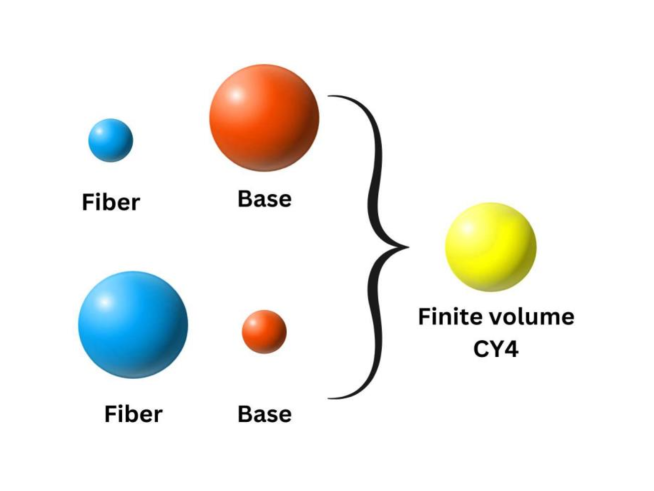
Figure 1: Graphic representation of the volumes of the fiber and the base of the two K3 surfaces making the Calabi-Yau fourfold.

As a result of this description, we cite the two following:

$\mathbf{1)}$

Given the fibration $X_{4}=S_{\bot}\times S_{\|},$ the volumes of the fibral surface $S_{\bot}$ and the base $S_{\|}$ of the fibered Calabi-Yau fourfold scales in terms of the spectral parameter $\textstyle\mathchar 277\relax$ like

$$vol\left(S_{\bot}\right)=\frac{1}{{{}\mathchoice{\mbox{\boldmath$\displaystyle\mathchar 277\relax$}}{\mbox{\boldmath$\textstyle\mathchar 277\relax$}}{\mbox{\boldmath$\scriptstyle\mathchar 277\relax$}}{\mbox{\boldmath$\scriptscriptstyle\mathchar 277\relax$}}}^{2}}\mathcal{V}_{K3_{\perp}}\quad,\quad vol\left(S_{\|}\right)={{}\mathchoice{\mbox{\boldmath$\displaystyle\mathchar 277\relax$}}{\mbox{\boldmath$\textstyle\mathchar 277\relax$}}{\mbox{\boldmath$\scriptstyle\mathchar 277\relax$}}{\mbox{\boldmath$\scriptscriptstyle\mathchar 277\relax$}}}^{2}\mathcal{V}_{K3_{\parallel}}\quad,\quad vol\left(X_{4}\right)\simeq\mathcal{V}_{K3_{\parallel}}\times\mathcal{V}_{K3_{\perp}}$$ (119)

From this behavior, we see that the volumes $vol\left(S_{\bot}\right)$ and $vol\left(S_{\|}\right)$ take singular values in the limits ${{}\mathchoice{\mbox{\boldmath$\displaystyle\mathchar 277\relax$}}{\mbox{\boldmath$\textstyle\mathchar 277\relax$}}{\mbox{\boldmath$\scriptstyle\mathchar 277\relax$}}{\mbox{\boldmath$\scriptscriptstyle\mathchar 277\relax$}}}\rightarrow\infty$ and ${{}\mathchoice{\mbox{\boldmath$\displaystyle\mathchar 277\relax$}}{\mbox{\boldmath$\textstyle\mathchar 277\relax$}}{\mbox{\boldmath$\scriptstyle\mathchar 277\relax$}}{\mbox{\boldmath$\scriptscriptstyle\mathchar 277\relax$}}}\rightarrow 0$; whilst the total volume of the Calabi-Yau fourfold $S_{\bot}\times S_{\|}$ remains finite.

$\mathbf{2)}$

Moreover, for ${{}\mathchoice{\mbox{\boldmath$\displaystyle\mathchar 277\relax$}}{\mbox{\boldmath$\textstyle\mathchar 277\relax$}}{\mbox{\boldmath$\scriptstyle\mathchar 277\relax$}}{\mbox{\boldmath$\scriptscriptstyle\mathchar 277\relax$}}}\rightarrow\infty,$ the $vol\left(S_{\bot}\right)$ shrinks ($vol\left(S_{\bot}\right)\rightarrow 0$) while the $vol\left(S_{\|}\right)$ diverges ($vol\left(S_{\|}\right)\rightarrow\infty$); this gives the Asymptotic weak coupling [$\mathcal{G}_{\|\|}^{weak}\int_{M_{3D}}\left(F^{\|}\wedge\ast F^{\|}\right)$] with gauge coupling metric

$$\mathcal{G}_{\|\|}^{weak}=\frac{1}{{{}\mathchoice{\mbox{\boldmath$\displaystyle\mathchar 277\relax$}}{\mbox{\boldmath$\textstyle\mathchar 277\relax$}}{\mbox{\boldmath$\scriptstyle\mathchar 277\relax$}}{\mbox{\boldmath$\scriptscriptstyle\mathchar 277\relax$}}}^{2}}G_{\|\|}$$ (120)

with asymptotic behavior as $\mathcal{G}_{\|\|}^{weak}\sim\mathcal{O}\left(1/{{}\mathchoice{\mbox{\boldmath$\displaystyle\mathchar 277\relax$}}{\mbox{\boldmath$\textstyle\mathchar 277\relax$}}{\mbox{\boldmath$\scriptstyle\mathchar 277\relax$}}{\mbox{\boldmath$\scriptscriptstyle\mathchar 277\relax$}}}^{2}\right)\rightarrow 0$. However, for $\left(1/{{}\mathchoice{\mbox{\boldmath$\displaystyle\mathchar 277\relax$}}{\mbox{\boldmath$\textstyle\mathchar 277\relax$}}{\mbox{\boldmath$\scriptstyle\mathchar 277\relax$}}{\mbox{\boldmath$\scriptscriptstyle\mathchar 277\relax$}}}\right)\rightarrow\infty,$ we have the inverse picture; the $vol\left(S_{\|}\right)$ shrinks but the $vol\left(S_{\bot}\right)$ diverges. The coupling [$\mathcal{G}_{\bot\bot}^{strong}\int_{M_{3D}}\left(F^{\bot}\wedge\ast F^{\bot}\right)$] has a ”strong coupling” metric

$$\mathcal{G}_{\bot\bot}^{strong}={{}\mathchoice{\mbox{\boldmath$\displaystyle\mathchar 277\relax$}}{\mbox{\boldmath$\textstyle\mathchar 277\relax$}}{\mbox{\boldmath$\scriptstyle\mathchar 277\relax$}}{\mbox{\boldmath$\scriptscriptstyle\mathchar 277\relax$}}}^{2}G_{\bot\bot}$$ (121)

with behavior at infinite distance $\mathcal{G}_{\bot\bot}^{strong}\sim\mathcal{O}\left({{}\mathchoice{\mbox{\boldmath$\displaystyle\mathchar 277\relax$}}{\mbox{\boldmath$\textstyle\mathchar 277\relax$}}{\mbox{\boldmath$\scriptstyle\mathchar 277\relax$}}{\mbox{\boldmath$\scriptscriptstyle\mathchar 277\relax$}}}^{2}\right)\rightarrow\infty.$ Because the change ${{}\mathchoice{\mbox{\boldmath$\displaystyle\mathchar 277\relax$}}{\mbox{\boldmath$\textstyle\mathchar 277\relax$}}{\mbox{\boldmath$\scriptstyle\mathchar 277\relax$}}{\mbox{\boldmath$\scriptscriptstyle\mathchar 277\relax$}}}\leftrightarrow 1/{{}\mathchoice{\mbox{\boldmath$\displaystyle\mathchar 277\relax$}}{\mbox{\boldmath$\textstyle\mathchar 277\relax$}}{\mbox{\boldmath$\scriptstyle\mathchar 277\relax$}}{\mbox{\boldmath$\scriptscriptstyle\mathchar 277\relax$}}}$ is a symmetry of the Kahler 2-form (112) and the EFT_3D, the asymptotic weak $\mathcal{G}_{\parallel\parallel}^{weak}$ and the short distance $\mathcal{G}_{\perp\perp}^{strong}$ are dual in M-theory on $K3_{\perp}\times K3_{\parallel}$.

$\mathbf{3)}$

In the infinite distance limit (${{}\mathchoice{\mbox{\boldmath$\displaystyle\mathchar 277\relax$}}{\mbox{\boldmath$\textstyle\mathchar 277\relax$}}{\mbox{\boldmath$\scriptstyle\mathchar 277\relax$}}{\mbox{\boldmath$\scriptscriptstyle\mathchar 277\relax$}}}\rightarrow\infty$), the fibral surface $S_{\bot}$ shrinks; and there exists a non singular curve $\Upsilon_{\mathbf{q}_{\perp}}$ in the fiber with charge $q_{\text{{a}}}=(q_{i_{\bot}};q_{a_{\|}}=0)$ where sits the weak gauge symmetry U$\left(1\right)_{weak}$. The complete curve $\Upsilon_{\mathbf{q}}$ in the CY4 is then fully located in $K3_{\perp}.$ By Weak/Strong gauge duality, we have a curve $\Upsilon_{\mathbf{q}_{\parallel}}$ and an abelian strong gauge symmetry U$\left(1\right)_{strong}$ lying in the base.

From these results, we conjecture that in the EFT_3D descending from M-theory on $K3_{\perp}\times K3_{\parallel}$ with the symmetry (111), we have two dual (weak and strong) asymptotic gauge regimes; the asymptotic strong gauge regime is the image of the asymptotic WGC under (111). Recall that asymptotic WGC stipulates that weakly coupled directions in the fibral $K3_{\perp}$ charge lattice host towers of BPS or non-BPS states which satisfy the weak gravity conjecture. By using the weak/strong duality ($K3_{\perp}\leftrightarrow K3_{\parallel})$, we expect to also have towers of BPS or non-BPS states in the strong gauge regime.

4.2 BPS and non BPS towers

As a consequence of the duality (111), the weakly coupled tower of BPS ($\mathcal{T}_{\mathrm{k}_{\mathrm{\bot}}\mathrm{,}\mathbf{q}_{\bot}}^{\text{{bps}}}$) or tower of non-BPS ($\mathcal{T}_{\mathrm{k}_{\mathrm{\bot}}\mathrm{,}\mathbf{q}_{\bot}}^{\text{{n-bps}}}$) states in the EFT${}_{3D}.$ These towers are predicted by the Asymptotic WGC conjecture (${{}\mathchoice{\mbox{\boldmath$\displaystyle\mathchar 277\relax$}}{\mbox{\boldmath$\textstyle\mathchar 277\relax$}}{\mbox{\boldmath$\scriptstyle\mathchar 277\relax$}}{\mbox{\boldmath$\scriptscriptstyle\mathchar 277\relax$}}}\rightarrow\infty$); they gets mapped under (111) into strongly coupled towers of BPS ($\mathcal{T}_{\mathrm{k}_{\mathrm{\|}}\mathrm{,}\mathbf{q}_{\|}}^{\text{{bps}}}$) or tower of non-BPS ($\mathcal{T}_{\mathrm{k}_{\mathrm{\|}}\mathrm{,}\mathbf{q}_{\|}}^{\text{{n-bps}}}$) states for the limit $\frac{1}{{{}\mathchoice{\mbox{\boldmath$\displaystyle\mathchar 277\relax$}}{\mbox{\boldmath$\textstyle\mathchar 277\relax$}}{\mbox{\boldmath$\scriptstyle\mathchar 277\relax$}}{\mbox{\boldmath$\scriptscriptstyle\mathchar 277\relax$}}}}\rightarrow\infty.$ This correspondence between the two gauge regimes (weak and strong) can be stated as follows

weak regime: $$g_{weak}^{2}$$ strong regime:

BPS_⊥ BPS_∥

non-BPS_⊥ non-BPS_∥

(122)

with $g_{weak}^{2}=\left(g_{{}_{\Upsilon}}^{2}\right)_{\perp\perp}$ and $g_{strong}^{2}=\left(g_{{}_{\Upsilon}}^{2}\right)_{\parallel\parallel}$. This result can be also motivated by the automorphism symmetry of $X_{4}=K3_{\parallel}\times K3_{\bot}$ exchanging the fiber $K3_{\bot}$ and the base $K3_{\parallel}.$

From the Table (122) and borrowing results from 12 , regarding EFT_5D induced from M-theory CY3 with K3 fibration, we learn that the EFT_3D descending from M-theory on $K3_{\parallel}\times K3_{\bot},$ that there are various towers of states satisfying the WGC and its gauge dual under (111).

The first towers are given by $\mathcal{T}_{\mathrm{k}_{\mathrm{\bot}}\mathrm{,}\mathbf{q}_{\bot}}^{\text{{bps}}}$ and $\mathcal{T}_{\mathrm{k}_{\mathrm{\|}}\mathrm{,}\mathbf{q}_{\|}}^{\text{{bps}}}$ and are dual: $\left(i\right)$ The $\mathcal{T}_{\mathrm{k}_{\mathrm{\bot}}\mathrm{,}\mathbf{q}_{\bot}}^{\text{{bps}}}$ is labeled by the integer $\mathrm{k}_{\mathrm{\bot}}$ and the charge vector $\mathbf{q}_{\bot}=\left(q_{1_{\bot}},...,q_{r_{\bot}}\right);$ it englobes BPS particle states $\left|BPS|_{\bot}\right\rangle$ constructed from M2 brane wrapped $k_{\bot}$ times around $\Upsilon_{\mathbf{q}_{\perp}}$ [BPS$|$${}_{\bot}=\text{M2/}\Upsilon_{\mathbf{q}_{\perp}}$]. The particle states generated have charges $\mathbf{Q}_{\perp}=\mathrm{k}_{\bot}\mathbf{q}_{\perp}$. By using Weak/Strong gauge duality, we get the dual tower $\mathcal{T}_{\mathrm{k}_{\mathrm{\|}}\mathrm{,}\mathbf{q}_{\|}}^{\text{{bps}}}$ of BPS states $\left|BPS|_{\parallel}\right\rangle$; it is given by wrapped M2 brane (BPS$|$${}_{\parallel}=\text{M2/}\Upsilon_{\mathbf{q}_{\parallel}}$) with charges$\ \mathbf{Q}_{\parallel}=\mathrm{k}_{\parallel}\mathbf{q}_{\parallel}$ as shown by the following table,

weak regime: $$g_{weak}^{2}$$ strong regime:

BPS BPS

(123)

Recall that the $\Upsilon_{\mathbf{q}_{\perp}}$ is purely fibral sitting in $K3_{\bot};$ it solves the condition (73) and has a positive self-intersection

$$\Upsilon_{\mathbf{q}_{\perp}}\equiv\mathcal{C}_{{\small U(1)}_{weak}},\qquad[\mathcal{C}_{{\small U(1)}_{weak}}]^{2}>0$$ (124)

whereas, the $\Upsilon_{\mathbf{q}_{\parallel}}$ is a purely base curve sitting in $K3_{\parallel};$ it satisfies the dual of the condition (73) and also has a positive self-intersection

$$\Upsilon_{\mathbf{q}_{\parallel}}\equiv\mathcal{C}_{{\small U(1)}_{strong}},\qquad[\mathcal{C}_{{\small U(1)}_{strong}}]^{2}>0$$ (125)

The second towers are given by $\mathcal{T}_{\mathrm{k}_{\mathrm{\bot}}\mathrm{,}\mathbf{q}_{\bot}}^{\text{{n-bps}}}$ and $\mathcal{T}_{\mathrm{k}_{\mathrm{\|}}\mathrm{,}\mathbf{q}_{\|}}^{\text{{n-bps}}}$ contain non-BPS particle states; these two towers are also dual under (111). Here, the non-BPS particles are given by excitations of Heterotic string. This string is dual to the so called MSW string given by M5 brane wrapping the fiber $K3$ 12 ; 26 . These are non-BPS states characterised by curves $\Upsilon_{\mathbf{Q}}$ in K3 with negative self-intersection ($\Upsilon_{\mathbf{Q}}^{2}<0)$. Depending on where we are considering the fiber K3_⊥ or the base K3, we distinguish two kinds of heterotic strings and then,

$$\text{M5/K3}_{\bot}$$ Het. string_⊥

Het. string_∥

(126)

The M-theory/heterotic string duality is explicitly formulated through the relation between the left moving excitations $n_{L}$ of the heterotic string and the self intersection of the curves $\Upsilon_{\mathbf{q}}$ 12 . Because $X_{4}=K3_{\parallel}\times K3_{\bot},$ we have

$$n_{L_{\perp}}$$

(127)

Having explored the weak/strong gauge duality in the EFT_3D, we turn now to investigate the asymptotic WGC in 3D. We present the conjecture in addition to its viability constraints in claim I and claim II; then we explicitly verify the conjecture for the different towers of states.

5 The Asymptotic WGC and weak/strong duality

In this section, we give two claims (I and II) for Asymptotic WGC in the EFT_3D considered in this paper. These claims generalise results obtained in five dimensional EFT_5D descending from M-theory on Calabi-Yau threefolds. We also give new results for the towers of BPS and non-BPS states in EFT_3D.

We start by noticing that since it was first proposed, the WGC has been formulated in different ways and refined multiple times. The basic version of the WGC in D-dimensions can be written as

$$m^{2}\leq\frac{D-2}{D-3}g^{2}q^{2}M_{\mathrm{Pl}}^{D-2}$$ (128)

Clearly this condition holds for $D>3;$ however investigations of the conjecture has been also performed in 3D; we cite for example 9A ; 9B where the WGC has been studied from the context of infrared consistency, and the condition of the WGC in 3D was expressed as

$$z^{2}\geq\frac{1}{2},\qquad z^{2}=\frac{q^{2}g^{2}}{m^{2}}M_{\mathrm{Pl}}$$ (129)

This constraints reads like

$$m^{2}\leq 2g^{2}q^{2}M_{Pl}$$ (130)

and is nothing but the (128) with the factor $(D-2)/(D-3)$ replaced by a factor of 2. Moreover, seen that 3D gravity is especially interesting in the context of AdS₃/CFT₂, it is important to mention the study conducted in 14G where the WGC has been formulated as follows

$$\Delta=\tilde{\Delta}=\frac{\mathrm{{{}\mathchoice{\mbox{\boldmath$\displaystyle\mathchar 267\relax$}}{\mbox{\boldmath$\textstyle\mathchar 267\relax$}}{\mbox{\boldmath$\scriptstyle\mathchar 267\relax$}}{\mbox{\boldmath$\scriptscriptstyle\mathchar 267\relax$}}}}^{\prime}}{4}m^{2}\leq\frac{1}{2}\max\left(Q^{2},\tilde{Q}^{2}\right)$$ (131)

where

$$\Delta=L_{0}-\frac{c}{24},\qquad\tilde{\Delta}=\tilde{L}_{0}-\frac{c}{24}$$ (132)

with $Q,$ $\tilde{Q}$ being the charges of the right and left movers respectively. If we substitute $\mathrm{{{}\mathchoice{\mbox{\boldmath$\displaystyle\mathchar 267\relax$}}{\mbox{\boldmath$\textstyle\mathchar 267\relax$}}{\mbox{\boldmath$\scriptstyle\mathchar 267\relax$}}{\mbox{\boldmath$\scriptscriptstyle\mathchar 267\relax$}}}}^{\prime}$ by 1/$M_{\mathrm{Pl}}$ and $\max(Q^{2},\tilde{Q}^{2})$ by $q^{2},$ then the WGC conjecture in 3D takes the form

$$m^{2}\leq 2g^{2}q^{2}M_{\mathrm{Pl}}$$ (133)

Given these facts, we come now to the 3D effective gauge theory coupled to gravity with typical field action as given by eq(41). In this theory, every direction $\Upsilon_{\mathrm{k}\mathbf{q}}$ in the even integral charge lattice $\mathfrak{L}_{K3_{\parallel}\times K3_{\bot}}$, that is dual to weakly coupled gauge group $U(1)_{weak}=U(1)_{\bot}$ [sometimes also denoted as $U(1)_{\Upsilon_{\mathrm{k}\mathbf{q}}}$], there exists a tower $\mathcal{T}_{\mathrm{k,}\mathbf{q}}$ of massive particle states $\left|\mathrm{k;}\mathbf{q;}M_{\mathrm{k}}\right\rangle$ that satisfy the inequality

$$M_{\mathrm{k}}^{2}\leq 2\mathrm{g}_{{\small 3D}}^{2}M_{\mathrm{Pl}}(q_{\text{{a}}}\mathcal{G}^{\text{{ab}}}q_{\text{{b}}})\mathrm{k}^{2}-\frac{1}{4}\mathfrak{g}^{\text{{xy}}}\frac{\partial M_{\mathrm{k}}}{\partial{{}\mathchoice{\mbox{\boldmath$\displaystyle\mathchar 286\relax$}}{\mbox{\boldmath$\textstyle\mathchar 286\relax$}}{\mbox{\boldmath$\scriptstyle\mathchar 286\relax$}}{\mbox{\boldmath$\scriptscriptstyle\mathchar 286\relax$}}}^{\text{{x}}}}\frac{\partial M_{\mathrm{k}}}{\partial{{}\mathchoice{\mbox{\boldmath$\displaystyle\mathchar 286\relax$}}{\mbox{\boldmath$\textstyle\mathchar 286\relax$}}{\mbox{\boldmath$\scriptstyle\mathchar 286\relax$}}{\mbox{\boldmath$\scriptscriptstyle\mathchar 286\relax$}}}^{\text{{y}}}}$$ (134)

In the inequality (134), the $\mathbf{q}=\left(q_{1},...,q_{r}\right)$ is integral charge vector and the other parameters have the canonical dimensions

$$\left[\mathrm{g}_{{\small 3D}}^{2}\right]=\left[M_{\mathrm{k}}\right]=mass^{1},\qquad\left[\mathcal{G}^{\text{{ab}}}\right]=\left[\mathfrak{g}^{\text{{xy}}}\right]=\left[{{}\mathchoice{\mbox{\boldmath$\displaystyle\mathchar 286\relax$}}{\mbox{\boldmath$\textstyle\mathchar 286\relax$}}{\mbox{\boldmath$\scriptstyle\mathchar 286\relax$}}{\mbox{\boldmath$\scriptscriptstyle\mathchar 286\relax$}}}^{\text{{x}}}\right]=mass^{0}$$ (135)

The $M_{\mathrm{k}}=M_{\mathrm{k}}\left({{}\mathchoice{\mbox{\boldmath$\displaystyle\mathchar 286\relax$}}{\mbox{\boldmath$\textstyle\mathchar 286\relax$}}{\mbox{\boldmath$\scriptstyle\mathchar 286\relax$}}{\mbox{\boldmath$\scriptscriptstyle\mathchar 286\relax$}}}\right)$ is the mass of the states in the BPS/non-BPS towers $\mathcal{T}_{\mathrm{k,}\mathbf{q}}^{\text{{bps}}}/\mathcal{T}_{\mathrm{k,}\mathbf{q}}^{\text{{n-bps}}};$ and the ${{}\mathchoice{\mbox{\boldmath$\displaystyle\mathchar 286\relax$}}{\mbox{\boldmath$\textstyle\mathchar 286\relax$}}{\mbox{\boldmath$\scriptstyle\mathchar 286\relax$}}{\mbox{\boldmath$\scriptscriptstyle\mathchar 286\relax$}}}^{\text{{x}}}$s are the scalar fields present in the EFT_3D that are responsible for the Yukawa attractive force $\mathfrak{g}^{\text{{xy}}}(\partial_{\text{{x}}}M_{\mathrm{k}})(\partial_{\text{{y}}}M_{\mathrm{k}})$. Moreover, the $\mathfrak{g}^{\text{{xy}}}$ is the inverse of the metric $\mathfrak{g}_{\text{{xy}}}$ of the scalar manifold of the EFT_3D. In what follows, we take all the volumes of the 2-cycles to be dimensionless in order to make the calculations easier; this is done by using the normalised variables $\hat{{{}\mathchoice{\mbox{\boldmath$\displaystyle\mathchar 285\relax$}}{\mbox{\boldmath$\textstyle\mathchar 285\relax$}}{\mbox{\boldmath$\scriptstyle\mathchar 285\relax$}}{\mbox{\boldmath$\scriptscriptstyle\mathchar 285\relax$}}}}^{\text{{a}}}={{}\mathchoice{\mbox{\boldmath$\displaystyle\mathchar 285\relax$}}{\mbox{\boldmath$\textstyle\mathchar 285\relax$}}{\mbox{\boldmath$\scriptstyle\mathchar 285\relax$}}{\mbox{\boldmath$\scriptscriptstyle\mathchar 285\relax$}}}^{\text{{a}}}/\mathcal{V}_{{\small CY}_{{\small 4}}}^{1/4}$ satisfying the property

$$\frac{1}{4!}{{}\mathchoice{\mbox{\boldmath$\displaystyle\mathchar 276\relax$}}{\mbox{\boldmath$\textstyle\mathchar 276\relax$}}{\mbox{\boldmath$\scriptstyle\mathchar 276\relax$}}{\mbox{\boldmath$\scriptscriptstyle\mathchar 276\relax$}}}_{\text{{abcd}}}\hat{{{}\mathchoice{\mbox{\boldmath$\displaystyle\mathchar 285\relax$}}{\mbox{\boldmath$\textstyle\mathchar 285\relax$}}{\mbox{\boldmath$\scriptstyle\mathchar 285\relax$}}{\mbox{\boldmath$\scriptscriptstyle\mathchar 285\relax$}}}}^{\text{{a}}}\hat{{{}\mathchoice{\mbox{\boldmath$\displaystyle\mathchar 285\relax$}}{\mbox{\boldmath$\textstyle\mathchar 285\relax$}}{\mbox{\boldmath$\scriptstyle\mathchar 285\relax$}}{\mbox{\boldmath$\scriptscriptstyle\mathchar 285\relax$}}}}^{\text{{b}}}\hat{{{}\mathchoice{\mbox{\boldmath$\displaystyle\mathchar 285\relax$}}{\mbox{\boldmath$\textstyle\mathchar 285\relax$}}{\mbox{\boldmath$\scriptstyle\mathchar 285\relax$}}{\mbox{\boldmath$\scriptscriptstyle\mathchar 285\relax$}}}}^{\text{{c}}}\hat{{{}\mathchoice{\mbox{\boldmath$\displaystyle\mathchar 285\relax$}}{\mbox{\boldmath$\textstyle\mathchar 285\relax$}}{\mbox{\boldmath$\scriptstyle\mathchar 285\relax$}}{\mbox{\boldmath$\scriptscriptstyle\mathchar 285\relax$}}}}^{\text{{d}}}=\widehat{\mathcal{V}}_{{\small CY}_{{\small 4}}}=1$$ (136)

To check the validity of the above inequality (134), we proceed in steps as follows:
First, we need to express the scalar field metric $\mathfrak{g}^{\text{{xy}}}$ in terms of the gauge coupling metric $\mathcal{G}^{\text{{ab}}}$ used before. This is achieved by help of the following formula

$$\mathfrak{g}_{\text{{xy}}}d{{}\mathchoice{\mbox{\boldmath$\displaystyle\mathchar 286\relax$}}{\mbox{\boldmath$\textstyle\mathchar 286\relax$}}{\mbox{\boldmath$\scriptstyle\mathchar 286\relax$}}{\mbox{\boldmath$\scriptscriptstyle\mathchar 286\relax$}}}^{\text{{x}}}\wedge\ast d{{}\mathchoice{\mbox{\boldmath$\displaystyle\mathchar 286\relax$}}{\mbox{\boldmath$\textstyle\mathchar 286\relax$}}{\mbox{\boldmath$\scriptstyle\mathchar 286\relax$}}{\mbox{\boldmath$\scriptscriptstyle\mathchar 286\relax$}}}^{\text{{y}}}$$

(137)

from which we deduce the relationship $\mathfrak{g}_{\text{{xy}}}=\mathcal{G}_{\text{{ab}}}(\partial_{\text{{x}}}\hat{{{}\mathchoice{\mbox{\boldmath$\displaystyle\mathchar 285\relax$}}{\mbox{\boldmath$\textstyle\mathchar 285\relax$}}{\mbox{\boldmath$\scriptstyle\mathchar 285\relax$}}{\mbox{\boldmath$\scriptscriptstyle\mathchar 285\relax$}}}}^{\text{{a}}})(\partial_{\text{{y}}}\hat{{{}\mathchoice{\mbox{\boldmath$\displaystyle\mathchar 285\relax$}}{\mbox{\boldmath$\textstyle\mathchar 285\relax$}}{\mbox{\boldmath$\scriptstyle\mathchar 285\relax$}}{\mbox{\boldmath$\scriptscriptstyle\mathchar 285\relax$}}}}^{\text{{b}}}).$ The inverse metric $\mathcal{G}^{\text{{ab}}}$ is related to the inverse $\mathfrak{g}^{\text{{xy}}}$ as follows

$$\mathcal{G}^{\text{{ab}}}=\frac{1}{2}\mathfrak{g}^{\text{{xy}}}(\partial_{\text{{x}}}\hat{{{}\mathchoice{\mbox{\boldmath$\displaystyle\mathchar 285\relax$}}{\mbox{\boldmath$\textstyle\mathchar 285\relax$}}{\mbox{\boldmath$\scriptstyle\mathchar 285\relax$}}{\mbox{\boldmath$\scriptscriptstyle\mathchar 285\relax$}}}}^{\text{{a}}})(\partial_{\text{{y}}}\hat{{{}\mathchoice{\mbox{\boldmath$\displaystyle\mathchar 285\relax$}}{\mbox{\boldmath$\textstyle\mathchar 285\relax$}}{\mbox{\boldmath$\scriptstyle\mathchar 285\relax$}}{\mbox{\boldmath$\scriptscriptstyle\mathchar 285\relax$}}}}^{\text{{b}}})+{{}\mathchoice{\mbox{\boldmath$\displaystyle\mathchar 293\relax$}}{\mbox{\boldmath$\textstyle\mathchar 293\relax$}}{\mbox{\boldmath$\scriptstyle\mathchar 293\relax$}}{\mbox{\boldmath$\scriptscriptstyle\mathchar 293\relax$}}}\hat{{{}\mathchoice{\mbox{\boldmath$\displaystyle\mathchar 285\relax$}}{\mbox{\boldmath$\textstyle\mathchar 285\relax$}}{\mbox{\boldmath$\scriptstyle\mathchar 285\relax$}}{\mbox{\boldmath$\scriptscriptstyle\mathchar 285\relax$}}}}^{\text{{a}}}\hat{{{}\mathchoice{\mbox{\boldmath$\displaystyle\mathchar 285\relax$}}{\mbox{\boldmath$\textstyle\mathchar 285\relax$}}{\mbox{\boldmath$\scriptstyle\mathchar 285\relax$}}{\mbox{\boldmath$\scriptscriptstyle\mathchar 285\relax$}}}}^{\text{{b}}}$$ (138)

with ${{}\mathchoice{\mbox{\boldmath$\displaystyle\mathchar 293\relax$}}{\mbox{\boldmath$\textstyle\mathchar 293\relax$}}{\mbox{\boldmath$\scriptstyle\mathchar 293\relax$}}{\mbox{\boldmath$\scriptscriptstyle\mathchar 293\relax$}}}=1/2.$ Using these variables, the Asymptotic WGC condition (134) reads in terms of $\mathcal{G}^{\text{{ab}}}$ then as follows

$$M_{\mathrm{k}}^{2}\leq 2\mathrm{g}_{{\small 3D}}^{2}M_{\mathrm{Pl}}(q_{\text{{a}}}\mathcal{G}^{\text{{ab}}}q_{\text{{b}}})\mathrm{k}^{2}-\frac{1}{2}(\mathcal{G}^{\text{{ab}}}-{{}\mathchoice{\mbox{\boldmath$\displaystyle\mathchar 293\relax$}}{\mbox{\boldmath$\textstyle\mathchar 293\relax$}}{\mbox{\boldmath$\scriptstyle\mathchar 293\relax$}}{\mbox{\boldmath$\scriptscriptstyle\mathchar 293\relax$}}}\hat{{{}\mathchoice{\mbox{\boldmath$\displaystyle\mathchar 285\relax$}}{\mbox{\boldmath$\textstyle\mathchar 285\relax$}}{\mbox{\boldmath$\scriptstyle\mathchar 285\relax$}}{\mbox{\boldmath$\scriptscriptstyle\mathchar 285\relax$}}}}^{\text{{a}}}\hat{{{}\mathchoice{\mbox{\boldmath$\displaystyle\mathchar 285\relax$}}{\mbox{\boldmath$\textstyle\mathchar 285\relax$}}{\mbox{\boldmath$\scriptstyle\mathchar 285\relax$}}{\mbox{\boldmath$\scriptscriptstyle\mathchar 285\relax$}}}}^{\text{{b}}})\frac{\partial M_{\mathrm{k}}}{\partial\hat{{{}\mathchoice{\mbox{\boldmath$\displaystyle\mathchar 285\relax$}}{\mbox{\boldmath$\textstyle\mathchar 285\relax$}}{\mbox{\boldmath$\scriptstyle\mathchar 285\relax$}}{\mbox{\boldmath$\scriptscriptstyle\mathchar 285\relax$}}}}^{\text{{a}}}}\frac{\partial M_{\mathrm{k}}}{\partial\hat{{{}\mathchoice{\mbox{\boldmath$\displaystyle\mathchar 285\relax$}}{\mbox{\boldmath$\textstyle\mathchar 285\relax$}}{\mbox{\boldmath$\scriptstyle\mathchar 285\relax$}}{\mbox{\boldmath$\scriptscriptstyle\mathchar 285\relax$}}}}^{\text{{b}}}}$$ (139)

Since our discussion is focusing on the Calabi-Yau fourfold fibration $CY_{4}=K3_{\perp}\times K3_{\parallel},$ we obtain a generalisation of the claims given in 12 for the case of EFT_5D descending from the Calabi-Yau threefold fibration $CY_{3}=K3\times\mathbb{B}_{1}$.

5.1 Two claims:  Weak/Strong gauge regimes

We give two claims (I and II); the claim-I concerns the asymptotic weak gauge coupling in the WGC; the claim-II regards the asymptotic strong gauge coupling in the WGC; it is the Weak/Strong gauge dual of the claim-I.

5.1.1 Claim-I: Weakly coupled regime

In M-theory compactified on $K3_{\perp}\times K3_{\parallel}$, for every direction in the associated even integral charge lattice $\mathfrak{L}=\mathfrak{L}_{\perp}\oplus\mathfrak{L}_{\parallel},$ with a primitive integral charge $\mathbf{q}=\mathbf{q}_{\perp}\oplus\mathbf{q}_{\parallel}$, we define two families of abelian gauge groups

$$U(1)_{\mathbf{q}_{\perp}}=\sum_{i_{\perp}=1}^{h_{\perp}^{1,1}}q_{i_{\perp}}U(1)^{i_{\perp}}\qquad,\qquad U(1)_{\mathbf{q}_{\parallel}}=\sum_{a_{\parallel}=1}^{h_{\parallel}^{1,1}}q_{a_{\parallel}}U(1)^{a_{\parallel}}$$ (140)

with the following properties:

(a)

Given the magnetic scale $\left(\Lambda_{{\small mag}}\right)_{U(1)_{\mathbf{q}_{\perp}}}$ and the species scale $\left(\Lambda_{\text{{sp}}}\right)_{{}_{U(1)_{\mathbf{q}_{\perp}}}},$ every direction $\mathbf{q}_{\perp}$ in the fibral lattice $\mathfrak{L}_{\perp}$ has a $U(1)_{\mathbf{q}_{\perp}}$ gauge factor with weak coupling limit in the infinite distance (${{}\mathchoice{\mbox{\boldmath$\displaystyle\mathchar 277\relax$}}{\mbox{\boldmath$\textstyle\mathchar 277\relax$}}{\mbox{\boldmath$\scriptstyle\mathchar 277\relax$}}{\mbox{\boldmath$\scriptscriptstyle\mathchar 277\relax$}}}\rightarrow\infty)$ in the sense

$$\left(\frac{\Lambda_{{\small mag}}}{\Lambda_{\text{{sp}}}}\right)_{U(1)_{\mathbf{q}_{\perp}}}\quad\rightarrow\quad 0,$$ (141)

admitting $\left(\mathbf{1}\right)$ either a tower $\mathcal{T}_{\mathrm{k_{\perp},}\mathbf{q}_{\perp}}^{\text{{bps}}}=\mathcal{T}_{M_{\mathrm{k_{\perp}}}\rightarrow 0}^{\text{{bps}}}$ of BPS states; or $\left(\mathbf{2}\right)$ a tower $\mathcal{T}_{\mathrm{k_{\perp},}\mathbf{q}_{\perp}}^{\text{{n-bps}}}=\mathcal{T}_{M_{\mathrm{k}_{{}_{\perp}}}\rightarrow 0}^{\text{{n-bps}}}$ of non-BPS states ($\mathrm{k_{\perp}}\in\mathbb{Z}$).

(b)

The BPS states, represented by the typical ket $\left|\mathrm{k_{\perp}};\mathbf{q_{\perp};}M_{\mathrm{k}_{\perp}}\right\rangle_{\text{{bps}}},$ are given M2- brane wrapping primitive 2-cycle $\Upsilon_{\mathbf{q}_{\perp}}^{\text{{bps}}}$ of the fiber $K3_{\perp}$ as illustrated by eqs(123-124). The complex curve $\mathbf{\Upsilon}_{\mathbf{q}_{\perp}}^{\text{{bps}}}$ (real 2-cycle associated with k${}_{\perp}=1$) has positive self intersection $\Upsilon_{\mathbf{q}_{\perp}}^{\text{{bps}}}.\Upsilon_{\mathbf{q}_{\perp}}^{\text{{bps}}}=\mathbf{q}_{\perp}^{2}>0;$ it sits in the even integral self dual sublattice $\mathfrak{L}_{\perp}^{\left(+\right)}$ of the fiber lattice $\mathfrak{L}_{\perp}$ having $\mathbf{q}_{\perp}^{2}=2m$ belonging to $2\mathbb{Z}.$ Moreover, each state in the tower $\mathcal{T}_{\mathrm{k_{\perp},}\mathbf{q}_{\perp}}^{\text{{bps}}},$ is characterised by the generic integer $\mathrm{k}_{\perp},$ which is given by M2- brane wrapping 2-cycles $\Upsilon_{\mathbf{q}_{\perp}}$ lying in $\mathfrak{L}_{\perp}^{\left(+\right)}$ multiple times.

(c)

The non-BPS states, represented by the typical ket $\left|n_{\mathbf{q}_{\perp}}^{L}\right\rangle_{\text{{n-bps}}},$ are given by heterotic string excitations as in (125-126); this string follows from the usual M-theory/heterotic duality. This heterotic string with left moving charge $n_{\mathbf{q}_{\perp}}^{L}$ is dual to the so-called Maldacena-Strominger-Witten (MSW) string given by M5 branes wrapping the generic fiber $K3_{\perp}.$ Here, the $K3_{\perp}$ contains a complex primitive curve $\Upsilon_{\mathbf{q}_{\perp}}^{\text{{n-bps}}}$ sitting in the anti-self dual sublattice $\mathfrak{L}_{\perp}^{\left(-\right)}$ with $\left(\mathbf{{{}\mathchoice{\mbox{\boldmath$\displaystyle\mathchar 267\relax$}}{\mbox{\boldmath$\textstyle\mathchar 267\relax$}}{\mbox{\boldmath$\scriptstyle\mathchar 267\relax$}}{\mbox{\boldmath$\scriptscriptstyle\mathchar 267\relax$}}}}\right)$ self intersection $\Upsilon_{\mathbf{q}_{\perp}}^{\text{{n-bps}}}.$ $\Upsilon_{\mathbf{q}_{\perp}}^{\text{{n-bps}}}=\mathbf{q}_{\perp}^{2}<0;$ and $\left(\mathbf{{{}\mathchoice{\mbox{\boldmath$\displaystyle\mathchar 268\relax$}}{\mbox{\boldmath$\textstyle\mathchar 268\relax$}}{\mbox{\boldmath$\scriptstyle\mathchar 268\relax$}}{\mbox{\boldmath$\scriptscriptstyle\mathchar 268\relax$}}}}\right)$ related to the string excitation charge as $n_{\mathbf{q}_{\perp}}^{L}=-\frac{1}{2}\mathbf{q}_{\perp}^{2}.$
Moreover, the tower $\mathcal{T}_{\mathrm{k_{\perp},}\mathbf{q}_{\perp}}^{\text{{n-bps}}}$ is characterised by the generic integer $\mathrm{k}_{\perp};$ as for the BPS case, the non BPS tower requires $K3_{\perp}$ containing complex curve $\Upsilon_{\mathrm{k}_{\perp}\mathbf{q}_{\perp}}=$ $\mathrm{k}_{\perp}\Upsilon_{\mathbf{q}_{\perp}}^{\text{{n-bps}}}$ sitting in the sublattice $\mathfrak{L}_{\perp}^{\left(-\right)}$ with self intersection $\mathbf{q}_{\perp}^{2}<0;$ and string excitation modes as

$$n_{\mathrm{k}_{\perp}\mathbf{q}_{\perp}}^{L}=-\frac{\mathrm{k}_{\perp}^{2}}{2}\mathbf{q}_{\perp}^{2}$$ (142)

Given the claim-I and the $\mathbb{Z}_{2}$ symmetry (111), we have the following dual claim-II assertion induced by Weak/strong gauge duality.

5.1.2 Claim-II: Strongly coupled regime

Because of the duality symmetry of the $CY_{4}=K3_{\perp}\times K3_{\parallel}$ acting by exchanging the two K3 surfaces ($K3_{\perp}\leftrightarrow K3_{\parallel}$), the properties given in Claim-I have a dual homologue. So, to every direction in the sublattice $\mathfrak{L}_{\parallel},$ dual to $\mathfrak{L}_{\perp},$ in the even integral charge lattice $\mathfrak{L}=\mathfrak{L}_{\perp}\oplus\mathfrak{L}_{\parallel}$; we have:

a)

a dual gauge symmetry factor $U(1)_{\mathbf{q}_{{}_{\parallel}}}$ with vector charge $\mathbf{q}_{{}_{\parallel}}=(q_{1_{\parallel}},...,q_{{{}\mathchoice{\mbox{\boldmath$\displaystyle\mathchar 279\relax$}}{\mbox{\boldmath$\textstyle\mathchar 279\relax$}}{\mbox{\boldmath$\scriptstyle\mathchar 279\relax$}}{\mbox{\boldmath$\scriptscriptstyle\mathchar 279\relax$}}}_{\parallel}})$ with strong gauge coupling limit in the sense,

$$\left(\frac{\Lambda_{{\small mag}}}{\Lambda_{\text{{sp}}}}\right)_{U(1)_{\mathbf{q}_{{}_{\parallel}}}}\quad\rightarrow\quad 0$$ (143)

admitting two towers of particle states in EFT${}_{{\small 3D}}:$ $\left(\mathbf{1}\right)$ a tower $\mathcal{T}_{\mathrm{k}_{{}_{\parallel}},\mathbf{q}_{{}_{\parallel}}}^{\text{{bps}}}=\mathcal{T}_{M_{\mathrm{k_{\parallel}}}\rightarrow 0}^{\text{{bps}}}$ of BPS particle states; or $\left(\mathbf{2}\right)$ a tower $\mathcal{T}_{\mathrm{k_{\parallel},}\mathbf{q}_{\parallel}}^{\text{{n-bps}}}=\mathcal{T}_{M_{\mathrm{k}_{{}_{\parallel}}}\rightarrow 0}^{\text{{n-bps}}}$ of non-BPS states. These two types of particles are described in the statements (b) and (c) given below.

b)

the BPS states $|\mathrm{k_{{}_{\parallel}};}\mathbf{q_{{}_{\parallel}};}M_{\mathrm{k}_{{}_{\parallel}}}>_{\text{{bps}}}$ are given M2 brane wrapping primitive 2-cycle $\Upsilon_{\mathbf{Q}_{{}_{\parallel}}}^{\text{{bps}}}$ of the base $K3_{{}_{\parallel}}$ with $\mathbf{Q}_{{}_{\parallel}}=\mathrm{k_{{}_{\parallel}}}\mathbf{q}_{{}_{\parallel}}.$ The cycle $\Upsilon_{\mathbf{q}_{{}_{\parallel}}}^{\text{{bps}}}$ (for the case k${}_{{}_{\parallel}}=1$) has positive self intersection with positive value $\mathbf{q}_{\parallel}^{2}>0$; it sits in the even integral ($\mathbf{q}_{\parallel}^{2}=2m_{\parallel}$) self dual sublattice $\mathfrak{L}_{\parallel}^{\left(+\right)}$ of the base lattice $\mathfrak{L}_{\parallel}.$
The tower $\mathcal{T}_{\mathrm{k}_{{}_{\parallel}},\mathbf{q}_{{}_{\parallel}}}^{\text{{bps}}}$ of BPS particles is characterised by the integer $\mathrm{k}_{{}_{\parallel}};$ it is generated by M2 brane wrapping the multi-2-cycles $\Upsilon_{\mathbf{Q}_{{}_{\parallel}}}=$ $\mathrm{k}_{\parallel}\Upsilon_{\mathbf{q}_{\parallel}}^{\text{{bps}}}$ expanding in the self dual sublattice $\mathfrak{L}_{\parallel}^{\left(+\right)}.$

c)

The non-BPS states $|n_{\mathbf{q}_{\parallel}}^{L}>_{\text{{n-bps}}}$ are given by the heterotic string excitations. The heterotic string with left moving charge $n_{\mathbf{q}_{\parallel}}^{L}$ is dual to the string given by M5 brane wrapping the base surface $K3_{\parallel}.$ Here, the $K3_{\parallel}$ contains a complex primitive curve $\Upsilon_{\mathbf{q}_{\parallel}}^{\text{{n-bps}}}$ sitting in the antiself dual sublattice $\mathfrak{L}_{\parallel}^{\left(-\right)}$ with $\left(\mathbf{{{}\mathchoice{\mbox{\boldmath$\displaystyle\mathchar 267\relax$}}{\mbox{\boldmath$\textstyle\mathchar 267\relax$}}{\mbox{\boldmath$\scriptstyle\mathchar 267\relax$}}{\mbox{\boldmath$\scriptscriptstyle\mathchar 267\relax$}}}}\right)$ negative self intersection value $\mathbf{q}_{\perp}^{2}<0;$ and $\left(\mathbf{{{}\mathchoice{\mbox{\boldmath$\displaystyle\mathchar 268\relax$}}{\mbox{\boldmath$\textstyle\mathchar 268\relax$}}{\mbox{\boldmath$\scriptstyle\mathchar 268\relax$}}{\mbox{\boldmath$\scriptscriptstyle\mathchar 268\relax$}}}}\right)$ related to the string excitation charge as $n_{\mathbf{q}_{\parallel}}^{L}=-\frac{1}{2}\mathbf{q}_{\parallel}^{2}>0.$
The tower $\mathcal{T}_{\mathrm{k}_{{}_{\parallel}},\mathbf{q}_{{}_{\parallel}}}^{\text{{n-bps}}}$ is characterised by the generic integer $\mathrm{k}_{\parallel};$ it requires $K3_{\parallel}$ having a complex curve $\Upsilon_{\mathbf{Q}_{\parallel}}=$ $k_{\parallel}\Upsilon_{\mathbf{q}_{\parallel}}^{\text{{n-bps}}}$ sitting in the sublattice $\mathfrak{L}_{\perp}^{\left(-\right)}$ with $\left(i\right)$ negative self intersection $\mathbf{q}_{\perp}^{2}<0;$ and $\left(ii\right)$ string excitation charge given by $n_{\mathrm{k}_{\parallel}\mathbf{q}_{\parallel}}^{L}=-\frac{\mathrm{k}_{\parallel}^{2}}{2}\mathbf{q}_{\parallel}^{2}.$

The complex curves $\Upsilon_{\perp}$ and $\Upsilon_{\parallel}$ used above depend on the structure of $K3_{\perp}\times K3_{\parallel},$ that is on whether they have degenerations at finite or infinite distance in the moduli space of the EFT_3D. Recall that in the EFT_5D investigated in 12 ; it was shown that in fibration of type K3, the only curves that admit a weak coupling are of two types: $\left(\mathbf{i}\right)$ K3 without degenerations; or $\left(\mathbf{ii}\right)$ curves that degenerate in a finite distance in the moduli space. These correspond to a generic K3 or degenerations classified as Kulikov type I, II or III 27A ; 27B . This result is general; and so hold also for our EFT_3D studied in this paper. In our claims given above, we mentioned that in directions of the charge lattice $\mathfrak{L}_{\perp}$ (resp. $\mathfrak{L}_{\parallel}$) that allow for a weak (or the dual strong) coupling limit, there exists towers of BPS or non-BPS states satisfying the WGC (or its strong dual version).
Notice that the BPS bound in the EFT_3D align with the extremality bound; and thus BPS states are super-extremal. This feature was shown for EFT_5D in particular in 28 ; there, the BPS states are all super-extremal, and satisfy the WGC, not only in the infinite distance limit (${{}\mathchoice{\mbox{\boldmath$\displaystyle\mathchar 277\relax$}}{\mbox{\boldmath$\textstyle\mathchar 277\relax$}}{\mbox{\boldmath$\scriptstyle\mathchar 277\relax$}}{\mbox{\boldmath$\scriptscriptstyle\mathchar 277\relax$}}}\rightarrow\infty$), but throughout the moduli space of the theory ($\textstyle\mathchar 277\relax$ finite); this is because charge to mass ratio is protected by supersymmetry. However, non-BPS states do not have this property.
In what follows, we test the conjecture for BPS and non-BPS states and weak/strong dual characterised by the conditions (141) and (143). We start by determining directions in the even integral charge lattice $\mathfrak{L}=\mathfrak{L}_{\perp}\oplus\mathfrak{L}_{\parallel}$ of the CY4 that admit a weak coupling limit. Then, we construct the towers $\mathcal{T}_{\mathrm{k},\mathbf{q}}^{\text{{bps}}}$ and $\mathcal{T}_{\mathrm{k},\mathbf{q}}^{\text{{n-bps}}}$ that host BPS and non-BPS states satisfying eqs(141-143).

5.2 Weakly/strongly coupled directions in the charge lattice

We start by focussing on the weak coupling limit at an infinite distance in the moduli space (${{}\mathchoice{\mbox{\boldmath$\displaystyle\mathchar 277\relax$}}{\mbox{\boldmath$\textstyle\mathchar 277\relax$}}{\mbox{\boldmath$\scriptstyle\mathchar 277\relax$}}{\mbox{\boldmath$\scriptscriptstyle\mathchar 277\relax$}}}\rightarrow\infty)$ of the EFT_3D; and turn after to investigating the strongly coupled region dual to asymptotic WGC. The asymptotic weak coupling limit is defined by the constraint relation (141) namely $\left(\Lambda_{{\small mag}}/\Lambda_{\text{{sp}}}\right)_{U(1)_{\mathbf{q}}}\rightarrow 0$ where $\Lambda_{{\small mag}}\equiv\Lambda_{\text{{wgc}}}$ is the magnetic WGC scale used earlier, and $\Lambda_{\text{{sp}}}\equiv\Lambda_{\text{{qg}}}$ is the species scale below which quantum gravity (QG) becomes weakly coupled. The reason that the weak gauge coupling limit is defined in such a way is because when approaching the species scale $\Lambda_{\text{{sp}}}$, the dynamics of quantum gravity change. Given a generic complex curve $\Upsilon_{\mathbf{q}}=\sum_{\text{{a}}=1}^{h_{{\small X}_{{\small 4}}}^{{\small 1,1}}}q_{\text{{a}}}\mathcal{C}^{\text{{a}}}$ in the Calabi-Yau fourfold $K3_{\perp}\times K3_{\parallel},$ the magnetic WGC scale in terms of the 3D Planck mass $M_{\mathrm{Pl}}$ and the Yang Mills gauge coupling $\mathrm{g}_{{\small 3D}}$ is defined as

$$\left.\Lambda_{{\small mag}}^{2}\right|_{\Upsilon_{\mathbf{q}}}=\mathrm{g}_{{\small 3D}}^{2}M_{\mathrm{Pl}}(q_{\text{{a}}}\mathcal{G}^{\text{{ab}}}q_{\text{{b}}})$$ (144)

Using the expression of the gauge coupling metric $\mathcal{G}^{\text{{ab}}}$ given by eq(85), this magnetic scale expands as follows

$$\left.\Lambda_{{\small mag}}^{2}\right|_{\Upsilon_{\mathbf{q}}} = {{}\mathchoice{\mbox{\boldmath$\displaystyle\mathchar 277\relax$}}{\mbox{\boldmath$\textstyle\mathchar 277\relax$}}{\mbox{\boldmath$\scriptstyle\mathchar 277\relax$}}{\mbox{\boldmath$\scriptscriptstyle\mathchar 277\relax$}}}^{2}\mathrm{g}_{{\small 3D}}^{2}M_{\mathrm{Pl}}(q_{a_{\parallel}}\mathring{G}^{a_{\parallel}b_{\parallel}}q_{b_{\parallel}})+$$

$$2{{}\mathchoice{\mbox{\boldmath$\displaystyle\mathchar 277\relax$}}{\mbox{\boldmath$\textstyle\mathchar 277\relax$}}{\mbox{\boldmath$\scriptstyle\mathchar 277\relax$}}{\mbox{\boldmath$\scriptscriptstyle\mathchar 277\relax$}}}^{0}\mathrm{g}_{{\small 3D}}^{2}M_{\mathrm{Pl}}(q_{a_{\parallel}}\mathring{G}^{a_{\parallel}i_{{}_{\perp}}}q_{i_{{}_{\perp}}})+$$

$$\frac{1}{{{}\mathchoice{\mbox{\boldmath$\displaystyle\mathchar 277\relax$}}{\mbox{\boldmath$\textstyle\mathchar 277\relax$}}{\mbox{\boldmath$\scriptstyle\mathchar 277\relax$}}{\mbox{\boldmath$\scriptscriptstyle\mathchar 277\relax$}}}^{2}}\mathrm{g}_{{\small 3D}}^{2}M_{\mathrm{Pl}}(q_{i_{\perp}}\mathring{G}^{i_{\perp}j_{\perp}}q_{j_{\perp}})$$

It has three block terms captured by diagonal coupling sub-matrices $\mathcal{G}^{i_{\perp}j_{\perp}}$ and $\mathcal{G}^{a_{\parallel}b_{\parallel}}$ as well as the cross block $\mathcal{G}^{a_{\parallel}i_{{}_{\perp}}}.$ From this expansion, we learn several features; in particular the two interesting following:

$\bullet$ Weakly gauge coupled directions
For fixed values of the scale $\Lambda_{\text{{sp}}},$ the weakly coupled directions in $K3_{\perp}\times K3_{\parallel}$ that realises the asymptotic weak gauge coupling condition $\left(\Lambda_{{\small mag}}/\Lambda_{\text{{sp}}}\right)_{U(1)_{\mathbf{q}}}\rightarrow 0$ is given by the necessary condition $\left.\Lambda_{{\small mag}}^{2}\right|_{\Upsilon_{\mathbf{q}}}\rightarrow 0.$ This necessary condition is solved in eq(5.2) by requiring

$$q_{a_{\parallel}}=0$$ (146)

thus restricting the complex curve $\mathbf{\Upsilon}_{\mathbf{q}}$ to sit completely in the fiber $K3_{\perp}$ of the CY₄; that is restricting $\Upsilon_{\mathbf{q}}$ to the fibral curve $\Upsilon_{\mathbf{q}_{\perp}}$ with expansion as $\sum_{i_{\perp}=1}^{h_{K3_{\perp}}^{{\small 1,1}}}q_{i_{\perp}}\mathcal{C}^{i_{\perp}}.$ With this restriction, eqs(144-5.2) read as follows

$$\left.\Lambda_{{\small mag}}^{2}\right|_{\Upsilon_{\mathbf{q}_{\perp}}}=\mathrm{g}_{{\small 3D}}^{2}(q_{i_{\perp}}\mathcal{G}^{i_{\perp}j_{\perp}}q_{j_{\perp}})=\frac{1}{{{}\mathchoice{\mbox{\boldmath$\displaystyle\mathchar 277\relax$}}{\mbox{\boldmath$\textstyle\mathchar 277\relax$}}{\mbox{\boldmath$\scriptstyle\mathchar 277\relax$}}{\mbox{\boldmath$\scriptscriptstyle\mathchar 277\relax$}}}^{2}}\mathrm{g}_{{\small 3D}}^{2}(q_{i_{\perp}}\mathring{G}^{i_{\perp}j_{\perp}}q_{j_{\perp}})$$ (147)

By setting $\mathrm{\mathring{g}}_{\Upsilon_{\mathbf{q}_{\perp}}}^{2}=\mathrm{g}_{{\small 3D}}^{2}(q_{i_{\perp}}\mathring{G}^{i_{\perp}j_{\perp}}q_{j_{\perp}})$ with no dependence in the scaling parameter ${{}\mathchoice{\mbox{\boldmath$\displaystyle\mathchar 277\relax$}}{\mbox{\boldmath$\textstyle\mathchar 277\relax$}}{\mbox{\boldmath$\scriptstyle\mathchar 277\relax$}}{\mbox{\boldmath$\scriptscriptstyle\mathchar 277\relax$}}},$ the above relation can be presented simply as

$$\left.\Lambda_{{\small mag}}^{2}\right|_{\Upsilon_{\mathbf{q}_{\perp}}}=\frac{1}{{{}\mathchoice{\mbox{\boldmath$\displaystyle\mathchar 277\relax$}}{\mbox{\boldmath$\textstyle\mathchar 277\relax$}}{\mbox{\boldmath$\scriptstyle\mathchar 277\relax$}}{\mbox{\boldmath$\scriptscriptstyle\mathchar 277\relax$}}}^{2}}\mathrm{\mathring{g}}_{\Upsilon_{\mathbf{q}_{\perp}}}^{2}$$ (148)

So, the magnetic scale behaves in the infinite distance limit (${{}\mathchoice{\mbox{\boldmath$\displaystyle\mathchar 277\relax$}}{\mbox{\boldmath$\textstyle\mathchar 277\relax$}}{\mbox{\boldmath$\scriptstyle\mathchar 277\relax$}}{\mbox{\boldmath$\scriptscriptstyle\mathchar 277\relax$}}}\rightarrow\infty)$ like

$$\left.\Lambda_{{\small mag}}^{2}\right|_{\Upsilon_{\mathbf{q}_{\perp}}}\sim\mathcal{O}\left(\frac{1}{{{}\mathchoice{\mbox{\boldmath$\displaystyle\mathchar 277\relax$}}{\mbox{\boldmath$\textstyle\mathchar 277\relax$}}{\mbox{\boldmath$\scriptstyle\mathchar 277\relax$}}{\mbox{\boldmath$\scriptscriptstyle\mathchar 277\relax$}}}^{2}}\right)\rightarrow 0$$ (149)

and then $\left(\Lambda_{{\small mag}}/\Lambda_{\text{{sp}}}\right)_{U(1)_{\mathbf{q}_{\perp}}}\rightarrow 0$.

$\bullet$ Strongly gauge coupled directions
For fixed values of $\Lambda_{\text{{sp}}},$ the strongly coupled directions in $K3_{\perp}\times K3_{\parallel},$ that are dual to the weak ones, realises the asymptotic strong coupling condition (LABEL:scf), the inverse of (141). This condition $\left(\Lambda_{{\small mag}}/\Lambda_{\text{{sp}}}\right)_{U(1)_{\mathbf{q}}}\rightarrow\infty$ can be realised by the necessary condition $\left.\Lambda_{mag}^{2}\right|_{\Upsilon_{\mathbf{q}}}\rightarrow\infty.$ From eq(144), we see that this necessary condition is naturally solved by demanding

$$q_{i_{\perp}}=0$$ (150)

thus restricting the complex curve $\Upsilon_{\mathbf{q}}$ to completely sitting in the base $K3_{\parallel}$ of the CY₄; that is restricting $\mathcal{\Upsilon}_{\mathbf{q}}$ to base curves $\Upsilon_{\mathbf{q}_{{}_{\parallel}}}$ given by $\sum_{a_{\parallel}=1}^{h_{K3\parallel}^{{\small 1,1}}}q_{a_{\parallel}}\mathcal{C}^{a_{\parallel}}.$ So the magnetic scale (144) reads as

$$\left.\Lambda_{{\small mag}}^{2}\right|_{\Upsilon_{\mathbf{q}_{\parallel}}}=\mathrm{g}_{{\small 3D}}^{2}M_{\mathrm{Pl}}(q_{a_{\parallel}}\mathcal{G}^{a_{\parallel}b_{\parallel}}q_{b_{\parallel}})={{}\mathchoice{\mbox{\boldmath$\displaystyle\mathchar 277\relax$}}{\mbox{\boldmath$\textstyle\mathchar 277\relax$}}{\mbox{\boldmath$\scriptstyle\mathchar 277\relax$}}{\mbox{\boldmath$\scriptscriptstyle\mathchar 277\relax$}}}^{2}\mathrm{g}_{{\small 3D}}^{2}M_{\mathrm{Pl}}(q_{a_{\parallel}}\mathring{G}^{a_{\parallel}b_{\parallel}}q_{b_{\parallel}})$$ (151)

By setting $\mathrm{\mathring{g}}_{\Upsilon_{\mathbf{n}_{\parallel}}}^{2}=\mathrm{g}_{{\small 3D}}^{2}(q_{a_{\parallel}}\mathring{G}^{a_{\parallel}b_{\parallel}}q_{b_{\parallel}})$ with finite dependence in the large limit of ${{}\mathchoice{\mbox{\boldmath$\displaystyle\mathchar 277\relax$}}{\mbox{\boldmath$\textstyle\mathchar 277\relax$}}{\mbox{\boldmath$\scriptstyle\mathchar 277\relax$}}{\mbox{\boldmath$\scriptscriptstyle\mathchar 277\relax$}}},$ this relation can be presented just like

$$\left.\Lambda_{{\small mag}}^{2}\right|_{\Upsilon_{\mathbf{q}_{\parallel}}}={{}\mathchoice{\mbox{\boldmath$\displaystyle\mathchar 277\relax$}}{\mbox{\boldmath$\textstyle\mathchar 277\relax$}}{\mbox{\boldmath$\scriptstyle\mathchar 277\relax$}}{\mbox{\boldmath$\scriptscriptstyle\mathchar 277\relax$}}}^{2}\mathrm{\mathring{g}}_{\Upsilon_{\mathbf{n}_{\parallel}}}^{2}$$ (152)

behaving like $\left.\Lambda_{{\small mag}}^{2}\right|_{\mathcal{\Upsilon}_{\mathbf{n}_{\parallel}}}\sim\mathcal{O}\left({{}\mathchoice{\mbox{\boldmath$\displaystyle\mathchar 277\relax$}}{\mbox{\boldmath$\textstyle\mathchar 277\relax$}}{\mbox{\boldmath$\scriptstyle\mathchar 277\relax$}}{\mbox{\boldmath$\scriptscriptstyle\mathchar 277\relax$}}}^{2}\right)$ and $\left.\Lambda_{{\small mag}}^{2}\right|_{\mathcal{\Upsilon}_{\mathbf{n}_{\parallel}}}\rightarrow\infty.$ Therefore, for fixed $\Lambda_{\text{{sp}}},$ we have $\left(\Lambda_{{\small mag}}/\Lambda_{\text{{sp}}}\right)_{U(1)_{\mathbf{q}_{\parallel}}}\rightarrow\infty.$

$\bullet$ About the species scale $\Lambda_{SP}$
First, recall that the species scale $\Lambda_{SP}$ is defined as the scale beyond which quantum gravity becomes strongly coupled. A general formula defining the species scale in D-dimensional space time is given by 3A ; 29

$$\Lambda_{\text{{sp}}}=\frac{M_{\mathrm{Pl}}^{{\tiny[D]}}}{N^{1/\left(D-2\right)}}$$ (153)

where $M_{\mathrm{Pl}}^{{\tiny[D]}}$ is the D-dimensional Planck mass, and $N$ is the number of species. In our EFT_3D descending from M-theory on $K3_{\perp}$-fibered Calabi-Yau fourfold on $K3_{\|}$, the species scale $\Lambda_{\text{{sp}}}$ and the heterotic scale $\mathrm{M}_{het}$ are linked by a logarithmic behaviour via

$$\Lambda_{\text{{sp}}}^{2}\sim\mathrm{M}_{{\small het}}^{2}\log(\frac{\mathrm{M}_{\mathrm{Pl}}}{\mathrm{M}_{{\small het}}})>0\qquad,\qquad\mathrm{M}_{{\small het}}<\mathrm{M}_{\mathrm{Pl}}$$ (154)

On the other hand taking the K3 volume $\mathcal{V}_{K3}$ to be dimensionless, the heterotic string tension $T_{het}=2{{}\mathchoice{\mbox{\boldmath$\displaystyle\mathchar 281\relax$}}{\mbox{\boldmath$\textstyle\mathchar 281\relax$}}{\mbox{\boldmath$\scriptstyle\mathchar 281\relax$}}{\mbox{\boldmath$\scriptscriptstyle\mathchar 281\relax$}}}\mathrm{M}_{het}^{2}$ is expressed in terms of the K3 volume as $T_{het}=2{{}\mathchoice{\mbox{\boldmath$\displaystyle\mathchar 281\relax$}}{\mbox{\boldmath$\textstyle\mathchar 281\relax$}}{\mbox{\boldmath$\scriptstyle\mathchar 281\relax$}}{\mbox{\boldmath$\scriptscriptstyle\mathchar 281\relax$}}}\mathcal{V}_{K3}\mathrm{M}_{11d}^{2}$ and then $\mathrm{M}_{{\small het}}^{2}=\mathrm{M}_{11d}^{2}\mathcal{V}_{K3}.$ So, we distinguish

$$\mathrm{M}_{{\small het}_{\perp}}^{2}=\mathrm{M}_{11d}^{2}\mathcal{V}_{X_{\perp}}\qquad,\qquad\mathrm{M}_{{\small het}_{\|}}^{2}=\mathrm{M}_{11d}^{2}\mathcal{V}_{K3_{{}_{\|}}}$$ (155)

Moreover, because under infinite distance scaling (${{}\mathchoice{\mbox{\boldmath$\displaystyle\mathchar 277\relax$}}{\mbox{\boldmath$\textstyle\mathchar 277\relax$}}{\mbox{\boldmath$\scriptstyle\mathchar 277\relax$}}{\mbox{\boldmath$\scriptscriptstyle\mathchar 277\relax$}}}\rightarrow\infty$), the volume $\mathcal{V}_{K3_{\perp}}$ of the fiber $K3_{\perp}$ scales like ${{}\mathchoice{\mbox{\boldmath$\displaystyle\mathchar 277\relax$}}{\mbox{\boldmath$\textstyle\mathchar 277\relax$}}{\mbox{\boldmath$\scriptstyle\mathchar 277\relax$}}{\mbox{\boldmath$\scriptscriptstyle\mathchar 277\relax$}}}^{-2}\mathcal{V}_{K3_{\perp}}$ while the volume $\mathcal{V}_{K3_{\|}}$ of the base $K3_{{}_{\|}}$ scales like ${{}\mathchoice{\mbox{\boldmath$\displaystyle\mathchar 277\relax$}}{\mbox{\boldmath$\textstyle\mathchar 277\relax$}}{\mbox{\boldmath$\scriptstyle\mathchar 277\relax$}}{\mbox{\boldmath$\scriptscriptstyle\mathchar 277\relax$}}}^{2}\mathcal{V}_{K3_{{}_{\|}}},$ the scaling of the heterotic mass scales $\mathrm{M}_{het\bot}$ and $\mathrm{M}_{het\|}$ respectively on the fiber and on the base of the CY4 behave as follows

$$\mathrm{M}_{het\bot}\sim\frac{1}{{{}\mathchoice{\mbox{\boldmath$\displaystyle\mathchar 277\relax$}}{\mbox{\boldmath$\textstyle\mathchar 277\relax$}}{\mbox{\boldmath$\scriptstyle\mathchar 277\relax$}}{\mbox{\boldmath$\scriptscriptstyle\mathchar 277\relax$}}}}\mathrm{M}_{11d}\qquad,\qquad\mathrm{M}_{het\|}\sim{{}\mathchoice{\mbox{\boldmath$\displaystyle\mathchar 277\relax$}}{\mbox{\boldmath$\textstyle\mathchar 277\relax$}}{\mbox{\boldmath$\scriptstyle\mathchar 277\relax$}}{\mbox{\boldmath$\scriptscriptstyle\mathchar 277\relax$}}}\mathrm{M}_{11d}$$ (156)

As such, in the infinite distance limit, we have $\mathrm{M}_{het\bot}\rightarrow 0$ while $\mathrm{M}_{het\|}\rightarrow\infty.$ By substituting into (154), the species scale $\Lambda_{\text{{sp}}_{\bot}}$ behaves for the asymptotic weak gauge coupling as

$$\Lambda_{\text{{sp}}_{\bot}}^{2}\sim\frac{\mathrm{M}_{11d}^{2}}{{{}\mathchoice{\mbox{\boldmath$\displaystyle\mathchar 277\relax$}}{\mbox{\boldmath$\textstyle\mathchar 277\relax$}}{\mbox{\boldmath$\scriptstyle\mathchar 277\relax$}}{\mbox{\boldmath$\scriptscriptstyle\mathchar 277\relax$}}}^{2}}\left[\log\frac{\mathrm{M}_{\mathrm{Pl}}}{\mathrm{M}_{11d}}+\log{{}\mathchoice{\mbox{\boldmath$\displaystyle\mathchar 277\relax$}}{\mbox{\boldmath$\textstyle\mathchar 277\relax$}}{\mbox{\boldmath$\scriptstyle\mathchar 277\relax$}}{\mbox{\boldmath$\scriptscriptstyle\mathchar 277\relax$}}}\right]$$ (157)

For the strongly coupled regions the species scale $\Lambda_{\text{{sp}}_{\|}}$ behaves like:

$$\Lambda_{\text{{sp}}_{\|}}^{2}\sim{{}\mathchoice{\mbox{\boldmath$\displaystyle\mathchar 277\relax$}}{\mbox{\boldmath$\textstyle\mathchar 277\relax$}}{\mbox{\boldmath$\scriptstyle\mathchar 277\relax$}}{\mbox{\boldmath$\scriptscriptstyle\mathchar 277\relax$}}}^{2}\mathrm{M}_{11d}^{2}\log\frac{\mathrm{M}_{\mathrm{Pl}}}{{{}\mathchoice{\mbox{\boldmath$\displaystyle\mathchar 277\relax$}}{\mbox{\boldmath$\textstyle\mathchar 277\relax$}}{\mbox{\boldmath$\scriptstyle\mathchar 277\relax$}}{\mbox{\boldmath$\scriptscriptstyle\mathchar 277\relax$}}}\mathrm{M}_{11d}}$$ (158)

indicating that we must have ${{}\mathchoice{\mbox{\boldmath$\displaystyle\mathchar 277\relax$}}{\mbox{\boldmath$\textstyle\mathchar 277\relax$}}{\mbox{\boldmath$\scriptstyle\mathchar 277\relax$}}{\mbox{\boldmath$\scriptscriptstyle\mathchar 277\relax$}}}\mathrm{M}_{11d}\leq\mathrm{M}_{\mathrm{Pl}}$ and then $\textstyle\mathchar 277\relax$ is bounded as ${{}\mathchoice{\mbox{\boldmath$\displaystyle\mathchar 277\relax$}}{\mbox{\boldmath$\textstyle\mathchar 277\relax$}}{\mbox{\boldmath$\scriptstyle\mathchar 277\relax$}}{\mbox{\boldmath$\scriptscriptstyle\mathchar 277\relax$}}}\leq\mathrm{M}_{\mathrm{Pl}}/\mathrm{M}_{11d}.$ Consequently, the asymptotic weak gauge coupling condition reading like

$$\frac{(\Lambda_{{\small mag}}^{2})_{{}_{\Upsilon_{\mathbf{q}_{\perp}}}}}{\Lambda_{\text{{sp}}_{\bot}}^{2}}=\frac{\mathrm{\mathring{g}}_{\Upsilon_{\mathbf{q}_{\perp}}}^{2}}{\mathrm{M}_{11d}\log{{}\mathchoice{\mbox{\boldmath$\displaystyle\mathchar 277\relax$}}{\mbox{\boldmath$\textstyle\mathchar 277\relax$}}{\mbox{\boldmath$\scriptstyle\mathchar 277\relax$}}{\mbox{\boldmath$\scriptscriptstyle\mathchar 277\relax$}}}}$$ (159)

tends indeed to zero in the infinite distance limit ${{}\mathchoice{\mbox{\boldmath$\displaystyle\mathchar 277\relax$}}{\mbox{\boldmath$\textstyle\mathchar 277\relax$}}{\mbox{\boldmath$\scriptstyle\mathchar 277\relax$}}{\mbox{\boldmath$\scriptscriptstyle\mathchar 277\relax$}}}\rightarrow\infty;$ thus showing the validity of the weak coupling limit condition (73-141). In this regards, it was shown in 12 that in fibration of type K3 of the CY3 of the EFT_5D, the curves $\mathcal{C}_{\mathbf{q}}$ that admit a weak gauge coupling symmetry $U\left(1\right)_{\mathcal{C}_{\mathbf{q}}}$ are either in a non degenerate fiber K3, or the ones that degenerate in a finite distance in the moduli space. This result is general since it only depends on the geometry of $K3$; and consequently holds also for the curves $\Upsilon_{\mathbf{q}_{\perp}}$ used in our EFT${}_{3D}\mathrm{.}$

As for the strongly coupled region, which is dual to the asymptotic weakly coupled region, the check of the condition is given by $\left(\Lambda_{{\small mag}}/\Lambda_{\text{{sp}}}\right)_{U(1)_{\mathbf{q}_{\parallel}}}\rightarrow\infty$ when the scaling parameter ${{}\mathchoice{\mbox{\boldmath$\displaystyle\mathchar 277\relax$}}{\mbox{\boldmath$\textstyle\mathchar 277\relax$}}{\mbox{\boldmath$\scriptstyle\mathchar 277\relax$}}{\mbox{\boldmath$\scriptscriptstyle\mathchar 277\relax$}}}\rightarrow\mathrm{M}_{\mathrm{Pl}}/\mathrm{M}_{11d}.$ By substituting $(\Lambda_{{\small mag}}^{2})_{\Upsilon_{\mathbf{q}_{\parallel}}}={{}\mathchoice{\mbox{\boldmath$\displaystyle\mathchar 277\relax$}}{\mbox{\boldmath$\textstyle\mathchar 277\relax$}}{\mbox{\boldmath$\scriptstyle\mathchar 277\relax$}}{\mbox{\boldmath$\scriptscriptstyle\mathchar 277\relax$}}}^{2}\mathrm{\mathring{g}}_{\Upsilon_{\mathbf{q}_{\parallel}}}^{2}$ and $\Lambda_{\text{{sp}}_{\|}}$ by its expression (158), the condition reads as follows

$$\frac{(\Lambda_{{\small mag}}^{2})_{\Upsilon_{\mathbf{q}_{\parallel}}}}{\Lambda_{\text{{sp}}_{\|}}^{2}}=\frac{\mathrm{\mathring{g}}_{\Upsilon_{\mathbf{q}_{\parallel}}}^{2}}{\mathrm{M}_{11d}^{2}\log\frac{\mathrm{M}_{\mathrm{Pl}}}{{{}\mathchoice{\mbox{\boldmath$\displaystyle\mathchar 277\relax$}}{\mbox{\boldmath$\textstyle\mathchar 277\relax$}}{\mbox{\boldmath$\scriptstyle\mathchar 277\relax$}}{\mbox{\boldmath$\scriptscriptstyle\mathchar 277\relax$}}}\mathrm{M}_{11d}}}$$ (160)

it tends to infinity for ${{}\mathchoice{\mbox{\boldmath$\displaystyle\mathchar 277\relax$}}{\mbox{\boldmath$\textstyle\mathchar 277\relax$}}{\mbox{\boldmath$\scriptstyle\mathchar 277\relax$}}{\mbox{\boldmath$\scriptscriptstyle\mathchar 277\relax$}}}\rightarrow\mathrm{M}_{\mathrm{Pl}}/\mathrm{M}_{11d}$ in agreement with the weak/strong duality property of the EFT_3D considered in this study.

In what follows we investigate the towers of states along these weak and strong directions in the charge lattice in $K3_{\|}\times K3_{\bot}.$ We start with the tower $\mathcal{T}_{\mathrm{k},\mathbf{q}}^{\text{{bps}}}$ BPS states in the EFT_3D, and then move on to the tower $\mathcal{T}_{\mathrm{k},\mathbf{q}}^{\text{{n-bps}}}$ of non-BPS states.

5.2.1 Towers of BPS states and asymptotic gauge couplings

Having determined the directions in the even integral charge lattice $\mathfrak{L}=\mathfrak{L}_{\perp}\oplus\mathfrak{L}_{\parallel}$ in the CY4 that are weakly coupled in $K3_{\bot}$ (and strongly in $K3_{\|}$ due to weak/gravity duality), we turn now to explicitly verify if the states in these directions satisfy the tower WGC and its strong dual version. To that purpose, recall that the WGC tower of states satisfies the relation (141); these states include BPS states occupying rays in the self dual sublattice $\mathfrak{L}_{\perp}^{\left(+\right)}$; and the non BPS states living in the anti-self dual $\mathfrak{L}_{\perp}^{\left(-\right)}.$

For the case of the BPS tower $\mathcal{T}_{\mathrm{k}_{\bot},\mathbf{q}_{\bot}}^{\text{{bps}}}$, it is built out of M2 brane wrapping complex curve $\Upsilon_{\mathrm{k}\mathbf{q}_{\bot}}$ in $\mathfrak{L}_{\perp}^{\left(+\right)}$ having positive self intersection ($\Upsilon_{\mathrm{k}_{\bot}\mathbf{q}_{\bot}}^{2}>0$). By weak/strong gauge duality, this feature extends naturally to a dual BPS tower $\mathcal{T}_{\mathrm{k}_{\|},\mathbf{q}_{\|}}^{\text{{bps}}}$ based on complex curves $\Upsilon_{\mathrm{k}_{\|}\mathbf{q}_{\|}}$ sitting in $\mathfrak{L}_{\|}^{\left(+\right)}$. For these two BPS towers, the masses $M_{\mathrm{k}}$ of their particle states is given by

$$M_{\mathrm{k}}={{}\mathchoice{\mbox{\boldmath$\displaystyle\mathchar 280\relax$}}{\mbox{\boldmath$\textstyle\mathchar 280\relax$}}{\mbox{\boldmath$\scriptstyle\mathchar 280\relax$}}{\mbox{\boldmath$\scriptscriptstyle\mathchar 280\relax$}}}M_{11d}\mathop{\displaystyle\sum}\limits_{\text{{a}}=1}^{h_{{\small CY4}}^{1,1}}\left(\mathrm{k}q_{\text{{a}}}\hat{{{}\mathchoice{\mbox{\boldmath$\displaystyle\mathchar 285\relax$}}{\mbox{\boldmath$\textstyle\mathchar 285\relax$}}{\mbox{\boldmath$\scriptstyle\mathchar 285\relax$}}{\mbox{\boldmath$\scriptscriptstyle\mathchar 285\relax$}}}}^{\text{{a}}}\right)\qquad,\qquad M_{11d}=\frac{M_{\mathrm{Pl}}}{\mathrm{{{}\mathchoice{\mbox{\boldmath$\displaystyle\mathchar 269\relax$}}{\mbox{\boldmath$\textstyle\mathchar 269\relax$}}{\mbox{\boldmath$\scriptstyle\mathchar 269\relax$}}{\mbox{\boldmath$\scriptscriptstyle\mathchar 269\relax$}}}}\mathcal{V}_{{\small CY}_{{\small 4}}}}$$ (161)

with integers k_x and dimensionless volume $\hat{{{}\mathchoice{\mbox{\boldmath$\displaystyle\mathchar 285\relax$}}{\mbox{\boldmath$\textstyle\mathchar 285\relax$}}{\mbox{\boldmath$\scriptstyle\mathchar 285\relax$}}{\mbox{\boldmath$\scriptscriptstyle\mathchar 285\relax$}}}}^{\text{{a}}}={{}\mathchoice{\mbox{\boldmath$\displaystyle\mathchar 285\relax$}}{\mbox{\boldmath$\textstyle\mathchar 285\relax$}}{\mbox{\boldmath$\scriptstyle\mathchar 285\relax$}}{\mbox{\boldmath$\scriptscriptstyle\mathchar 285\relax$}}}^{\text{{a}}}/\mathcal{V}_{{\small CY}_{4}}^{1/4}$ and $\mathrm{{{}\mathchoice{\mbox{\boldmath$\displaystyle\mathchar 269\relax$}}{\mbox{\boldmath$\textstyle\mathchar 269\relax$}}{\mbox{\boldmath$\scriptstyle\mathchar 269\relax$}}{\mbox{\boldmath$\scriptscriptstyle\mathchar 269\relax$}}}=4{{}\mathchoice{\mbox{\boldmath$\displaystyle\mathchar 281\relax$}}{\mbox{\boldmath$\textstyle\mathchar 281\relax$}}{\mbox{\boldmath$\scriptstyle\mathchar 281\relax$}}{\mbox{\boldmath$\scriptscriptstyle\mathchar 281\relax$}}}}$ and ${{}\mathchoice{\mbox{\boldmath$\displaystyle\mathchar 280\relax$}}{\mbox{\boldmath$\textstyle\mathchar 280\relax$}}{\mbox{\boldmath$\scriptstyle\mathchar 280\relax$}}{\mbox{\boldmath$\scriptscriptstyle\mathchar 280\relax$}}}=1/\sqrt{2}.$ From this expression of the mass, which splits like the sum of $M_{\mathrm{k}}=M_{\mathrm{k}_{\bot}}+M_{\mathrm{k}_{\|}}$ with

$$M_{\mathrm{k}_{\bot}}={{}\mathchoice{\mbox{\boldmath$\displaystyle\mathchar 280\relax$}}{\mbox{\boldmath$\textstyle\mathchar 280\relax$}}{\mbox{\boldmath$\scriptstyle\mathchar 280\relax$}}{\mbox{\boldmath$\scriptscriptstyle\mathchar 280\relax$}}}M_{11d}\sum_{i_{\bot}=1}^{h_{\bot}^{1,1}}\left(\mathrm{k}_{\bot}q_{i_{\bot}}\hat{{{}\mathchoice{\mbox{\boldmath$\displaystyle\mathchar 285\relax$}}{\mbox{\boldmath$\textstyle\mathchar 285\relax$}}{\mbox{\boldmath$\scriptstyle\mathchar 285\relax$}}{\mbox{\boldmath$\scriptscriptstyle\mathchar 285\relax$}}}}^{i_{\bot}}\right)\qquad,\qquad M_{\mathrm{k}_{\|}}={{}\mathchoice{\mbox{\boldmath$\displaystyle\mathchar 280\relax$}}{\mbox{\boldmath$\textstyle\mathchar 280\relax$}}{\mbox{\boldmath$\scriptstyle\mathchar 280\relax$}}{\mbox{\boldmath$\scriptscriptstyle\mathchar 280\relax$}}}M_{11d}\sum_{a_{\|}=1}^{h_{\|}^{1,1}}\left(\mathrm{k}_{\|}q_{a_{\|}}\hat{{{}\mathchoice{\mbox{\boldmath$\displaystyle\mathchar 285\relax$}}{\mbox{\boldmath$\textstyle\mathchar 285\relax$}}{\mbox{\boldmath$\scriptstyle\mathchar 285\relax$}}{\mbox{\boldmath$\scriptscriptstyle\mathchar 285\relax$}}}}^{a_{\|}}\right)$$ (162)

we can check the asymptotic WGC condition (141) and its strong regime dual (141).

Now, given eq(161), we learn that $M_{\mathrm{k}}^{2}$ is equal to $4{{}\mathchoice{\mbox{\boldmath$\displaystyle\mathchar 281\relax$}}{\mbox{\boldmath$\textstyle\mathchar 281\relax$}}{\mbox{\boldmath$\scriptstyle\mathchar 281\relax$}}{\mbox{\boldmath$\scriptscriptstyle\mathchar 281\relax$}}}^{2}\mathrm{k}^{2}\left(q_{\text{{a}}}\hat{{{}\mathchoice{\mbox{\boldmath$\displaystyle\mathchar 285\relax$}}{\mbox{\boldmath$\textstyle\mathchar 285\relax$}}{\mbox{\boldmath$\scriptstyle\mathchar 285\relax$}}{\mbox{\boldmath$\scriptscriptstyle\mathchar 285\relax$}}}}^{\text{{a}}}\right)^{2}M_{11d}^{2}$ , it is quadratic in the volumes $\hat{{{}\mathchoice{\mbox{\boldmath$\displaystyle\mathchar 285\relax$}}{\mbox{\boldmath$\textstyle\mathchar 285\relax$}}{\mbox{\boldmath$\scriptstyle\mathchar 285\relax$}}{\mbox{\boldmath$\scriptscriptstyle\mathchar 285\relax$}}}}^{\text{{a}}}$ and in $\mathrm{k}$ as well as the integral charges $q_{\text{{a}}}$; it splits into three blocks as follows

$$\left(M_{\mathrm{k}}\right)^{2}=\left(M_{\mathrm{k}_{\bot}}\right)^{2}+(M_{\mathrm{k}_{\|}})^{2}+2M_{\mathrm{k}_{\bot}}M_{\mathrm{k}_{\|}}$$ (163)

where the fibral $\left(M_{\mathrm{k}_{\bot}}\right)^{2}$ and the base $(M_{\mathrm{k}_{\|}})^{2}$ are quadratic in ($\hat{{{}\mathchoice{\mbox{\boldmath$\displaystyle\mathchar 285\relax$}}{\mbox{\boldmath$\textstyle\mathchar 285\relax$}}{\mbox{\boldmath$\scriptstyle\mathchar 285\relax$}}{\mbox{\boldmath$\scriptscriptstyle\mathchar 285\relax$}}}}^{i_{\bot}},\mathrm{k}_{\bot},q_{i_{\bot}})$ and ($\hat{{{}\mathchoice{\mbox{\boldmath$\displaystyle\mathchar 285\relax$}}{\mbox{\boldmath$\textstyle\mathchar 285\relax$}}{\mbox{\boldmath$\scriptstyle\mathchar 285\relax$}}{\mbox{\boldmath$\scriptscriptstyle\mathchar 285\relax$}}}}^{a_{\|}},\mathrm{k}_{\|},q_{a_{\|}})$ respectively.

A. Repulsive Force Conjecture (RFC):

Given a massive BPS particle in the EFT_3D of mass $M_{\mathrm{k}}$, the repulsive force conjecture (RFC), which in the infinite distance limit coincides with the asymptotic WGC, requires the following inequality 3A ; 6A ; 6B

$$F_{Coulomb}\geq F_{Grav}+F_{Yukawa}$$ (164)

This inequality reads explicitly as follows

$$\frac{\mathrm{g}_{{\small 3D}}^{2}}{M_{\mathrm{Pl}}}\left(\mathrm{k}^{2}q_{\text{{a}}}\mathcal{G}^{\text{{ab}}}q_{\text{{b}}}\right)\geq\left.\frac{D-3}{D-2}\right|_{D=3}\frac{M_{\mathrm{k}}^{2}}{M_{\mathrm{Pl}}^{2}}+\mathcal{Y}$$ (165)

with Yukawa matter coupling contribution $\mathcal{Y}$ reading in terms of the reduced mass $M_{\mathrm{k}}$ as follows

$$M_{\mathrm{Pl}}^{2}\mathcal{Y} = \frac{\mathcal{G}^{\text{{ab}}}}{2M_{\mathrm{k}}^{2}}\left(\frac{\partial M_{\mathrm{k}}^{2}}{\partial\hat{{{}\mathchoice{\mbox{\boldmath$\displaystyle\mathchar 285\relax$}}{\mbox{\boldmath$\textstyle\mathchar 285\relax$}}{\mbox{\boldmath$\scriptstyle\mathchar 285\relax$}}{\mbox{\boldmath$\scriptscriptstyle\mathchar 285\relax$}}}}^{\text{{a}}}}\right)\left(\frac{\partial M_{\mathrm{k}}^{2}}{\partial\hat{{{}\mathchoice{\mbox{\boldmath$\displaystyle\mathchar 285\relax$}}{\mbox{\boldmath$\textstyle\mathchar 285\relax$}}{\mbox{\boldmath$\scriptstyle\mathchar 285\relax$}}{\mbox{\boldmath$\scriptscriptstyle\mathchar 285\relax$}}}}^{\text{{b}}}}\right)-\frac{{{}\mathchoice{\mbox{\boldmath$\displaystyle\mathchar 293\relax$}}{\mbox{\boldmath$\textstyle\mathchar 293\relax$}}{\mbox{\boldmath$\scriptstyle\mathchar 293\relax$}}{\mbox{\boldmath$\scriptscriptstyle\mathchar 293\relax$}}}}{M_{\mathrm{k}}^{2}}\left[\hat{{{}\mathchoice{\mbox{\boldmath$\displaystyle\mathchar 285\relax$}}{\mbox{\boldmath$\textstyle\mathchar 285\relax$}}{\mbox{\boldmath$\scriptstyle\mathchar 285\relax$}}{\mbox{\boldmath$\scriptscriptstyle\mathchar 285\relax$}}}}^{\text{{a}}}\frac{\partial M_{\mathrm{k}}^{2}}{\partial\hat{{{}\mathchoice{\mbox{\boldmath$\displaystyle\mathchar 285\relax$}}{\mbox{\boldmath$\textstyle\mathchar 285\relax$}}{\mbox{\boldmath$\scriptstyle\mathchar 285\relax$}}{\mbox{\boldmath$\scriptscriptstyle\mathchar 285\relax$}}}}^{\text{{a}}}}\right]^{2}$$ (166)

$$= 2\mathcal{G}^{\text{{ab}}}\left(\frac{\partial M_{\mathrm{k}}}{\partial\hat{{{}\mathchoice{\mbox{\boldmath$\displaystyle\mathchar 285\relax$}}{\mbox{\boldmath$\textstyle\mathchar 285\relax$}}{\mbox{\boldmath$\scriptstyle\mathchar 285\relax$}}{\mbox{\boldmath$\scriptscriptstyle\mathchar 285\relax$}}}}^{\text{{a}}}}\right)\left(\frac{\partial M_{\mathrm{k}}}{\partial\hat{{{}\mathchoice{\mbox{\boldmath$\displaystyle\mathchar 285\relax$}}{\mbox{\boldmath$\textstyle\mathchar 285\relax$}}{\mbox{\boldmath$\scriptstyle\mathchar 285\relax$}}{\mbox{\boldmath$\scriptscriptstyle\mathchar 285\relax$}}}}^{\text{{b}}}}\right)-4{{}\mathchoice{\mbox{\boldmath$\displaystyle\mathchar 293\relax$}}{\mbox{\boldmath$\textstyle\mathchar 293\relax$}}{\mbox{\boldmath$\scriptstyle\mathchar 293\relax$}}{\mbox{\boldmath$\scriptscriptstyle\mathchar 293\relax$}}}\left[\hat{{{}\mathchoice{\mbox{\boldmath$\displaystyle\mathchar 285\relax$}}{\mbox{\boldmath$\textstyle\mathchar 285\relax$}}{\mbox{\boldmath$\scriptstyle\mathchar 285\relax$}}{\mbox{\boldmath$\scriptscriptstyle\mathchar 285\relax$}}}}^{\text{{a}}}\frac{\partial M_{\mathrm{k}}}{\partial\hat{{{}\mathchoice{\mbox{\boldmath$\displaystyle\mathchar 285\relax$}}{\mbox{\boldmath$\textstyle\mathchar 285\relax$}}{\mbox{\boldmath$\scriptstyle\mathchar 285\relax$}}{\mbox{\boldmath$\scriptscriptstyle\mathchar 285\relax$}}}}^{\text{{a}}}}\right]^{2}$$ (167)

with ${{}\mathchoice{\mbox{\boldmath$\displaystyle\mathchar 293\relax$}}{\mbox{\boldmath$\textstyle\mathchar 293\relax$}}{\mbox{\boldmath$\scriptstyle\mathchar 293\relax$}}{\mbox{\boldmath$\scriptscriptstyle\mathchar 293\relax$}}}=1/2.$ Notice that because here $D=3,$ the contribution from classical gravity namely $\left(D-3\right)/\left(D-2\right)$ vanishes identically; this is expected because massless 3D gravity is topological. However, a non trivial contribution may come from quantum effect; we denote it like $\mathrm{{{}\mathchoice{\mbox{\boldmath$\displaystyle\mathchar 291\relax$}}{\mbox{\boldmath$\textstyle\mathchar 291\relax$}}{\mbox{\boldmath$\scriptstyle\mathchar 291\relax$}}{\mbox{\boldmath$\scriptscriptstyle\mathchar 291\relax$}}}}_{{\small QG}}$. Substituting, the RFC inequality (165) becomes

$$\mathrm{g}_{{\small 3D}}^{2}M_{\mathrm{Pl}}\left(\mathrm{k}^{2}q_{\text{{a}}}\mathcal{G}^{\text{{ab}}}q_{\text{{b}}}\right)\geq\mathrm{{{}\mathchoice{\mbox{\boldmath$\displaystyle\mathchar 291\relax$}}{\mbox{\boldmath$\textstyle\mathchar 291\relax$}}{\mbox{\boldmath$\scriptstyle\mathchar 291\relax$}}{\mbox{\boldmath$\scriptscriptstyle\mathchar 291\relax$}}}}_{{\small QG}}+\frac{\mathcal{G}^{\text{{ab}}}}{2M_{\mathrm{k}}^{2}}\left(\frac{\partial M_{\mathrm{k}}^{2}}{\partial\hat{{{}\mathchoice{\mbox{\boldmath$\displaystyle\mathchar 285\relax$}}{\mbox{\boldmath$\textstyle\mathchar 285\relax$}}{\mbox{\boldmath$\scriptstyle\mathchar 285\relax$}}{\mbox{\boldmath$\scriptscriptstyle\mathchar 285\relax$}}}}^{\text{{a}}}}\right)\left(\frac{\partial M_{\mathrm{k}}^{2}}{\partial\hat{{{}\mathchoice{\mbox{\boldmath$\displaystyle\mathchar 285\relax$}}{\mbox{\boldmath$\textstyle\mathchar 285\relax$}}{\mbox{\boldmath$\scriptstyle\mathchar 285\relax$}}{\mbox{\boldmath$\scriptscriptstyle\mathchar 285\relax$}}}}^{\text{{b}}}}\right)-\frac{{{}\mathchoice{\mbox{\boldmath$\displaystyle\mathchar 293\relax$}}{\mbox{\boldmath$\textstyle\mathchar 293\relax$}}{\mbox{\boldmath$\scriptstyle\mathchar 293\relax$}}{\mbox{\boldmath$\scriptscriptstyle\mathchar 293\relax$}}}}{M_{\mathrm{k}}^{2}}\left[\hat{{{}\mathchoice{\mbox{\boldmath$\displaystyle\mathchar 285\relax$}}{\mbox{\boldmath$\textstyle\mathchar 285\relax$}}{\mbox{\boldmath$\scriptstyle\mathchar 285\relax$}}{\mbox{\boldmath$\scriptscriptstyle\mathchar 285\relax$}}}}^{\text{{a}}}\frac{\partial M_{\mathrm{k}}^{2}}{\partial\hat{{{}\mathchoice{\mbox{\boldmath$\displaystyle\mathchar 285\relax$}}{\mbox{\boldmath$\textstyle\mathchar 285\relax$}}{\mbox{\boldmath$\scriptstyle\mathchar 285\relax$}}{\mbox{\boldmath$\scriptscriptstyle\mathchar 285\relax$}}}}^{\text{{a}}}}\right]^{2}$$ (168)

with charge $q_{\text{{a}}}=\left(q_{i_{\perp}},q_{a_{\|}}\right).$ We rewrite this inequality by putting the mass contribution to the right hand side as follows

$$\frac{\mathrm{g}_{{\small 3D}}^{2}M_{\mathrm{Pl}}}{4}\left(\mathrm{k}^{2}q_{\text{{a}}}\mathcal{G}^{\text{{ab}}}q_{\text{{b}}}\right)\geq\mathrm{{{}\mathchoice{\mbox{\boldmath$\displaystyle\mathchar 291\relax$}}{\mbox{\boldmath$\textstyle\mathchar 291\relax$}}{\mbox{\boldmath$\scriptstyle\mathchar 291\relax$}}{\mbox{\boldmath$\scriptscriptstyle\mathchar 291\relax$}}}}_{{\small QG}}+\frac{1}{2}\mathcal{G}^{\text{{ab}}}\left(\frac{\partial M_{\mathrm{k}_{x}}}{\partial\hat{{{}\mathchoice{\mbox{\boldmath$\displaystyle\mathchar 285\relax$}}{\mbox{\boldmath$\textstyle\mathchar 285\relax$}}{\mbox{\boldmath$\scriptstyle\mathchar 285\relax$}}{\mbox{\boldmath$\scriptscriptstyle\mathchar 285\relax$}}}}^{\text{{a}}}}\right)\left(\frac{\partial M_{\mathrm{k}_{x}}}{\partial\hat{{{}\mathchoice{\mbox{\boldmath$\displaystyle\mathchar 285\relax$}}{\mbox{\boldmath$\textstyle\mathchar 285\relax$}}{\mbox{\boldmath$\scriptstyle\mathchar 285\relax$}}{\mbox{\boldmath$\scriptscriptstyle\mathchar 285\relax$}}}}^{\text{{b}}}}\right)-{{}\mathchoice{\mbox{\boldmath$\displaystyle\mathchar 293\relax$}}{\mbox{\boldmath$\textstyle\mathchar 293\relax$}}{\mbox{\boldmath$\scriptstyle\mathchar 293\relax$}}{\mbox{\boldmath$\scriptscriptstyle\mathchar 293\relax$}}}\left[\hat{{{}\mathchoice{\mbox{\boldmath$\displaystyle\mathchar 285\relax$}}{\mbox{\boldmath$\textstyle\mathchar 285\relax$}}{\mbox{\boldmath$\scriptstyle\mathchar 285\relax$}}{\mbox{\boldmath$\scriptscriptstyle\mathchar 285\relax$}}}}^{\text{{a}}}\frac{\partial M_{\mathrm{k}_{x}}}{\partial\hat{{{}\mathchoice{\mbox{\boldmath$\displaystyle\mathchar 285\relax$}}{\mbox{\boldmath$\textstyle\mathchar 285\relax$}}{\mbox{\boldmath$\scriptstyle\mathchar 285\relax$}}{\mbox{\boldmath$\scriptscriptstyle\mathchar 285\relax$}}}}^{\text{{a}}}}\right]^{2}$$ (169)

Because the metric inverse $\mathcal{G}^{\text{{ab}}}$ plays an important role in this relation and its test, we first give details on its calculation; and turn after to verify the validity of the repulsive force conjecture for the tower of BPS states. Below, we assume $\mathrm{{{}\mathchoice{\mbox{\boldmath$\displaystyle\mathchar 291\relax$}}{\mbox{\boldmath$\textstyle\mathchar 291\relax$}}{\mbox{\boldmath$\scriptstyle\mathchar 291\relax$}}{\mbox{\boldmath$\scriptscriptstyle\mathchar 291\relax$}}}}_{{\small QG}}<0$ for BPS particle states in vacuum TPA ; TPB ; so to test (168-169), we can disregard $\mathrm{{{}\mathchoice{\mbox{\boldmath$\displaystyle\mathchar 291\relax$}}{\mbox{\boldmath$\textstyle\mathchar 291\relax$}}{\mbox{\boldmath$\scriptstyle\mathchar 291\relax$}}{\mbox{\boldmath$\scriptscriptstyle\mathchar 291\relax$}}}}_{{\small QG}}$ without affection the message captured by the conjecture.

B.  Deriving the inverse of gauge metric (221):

In eq(204), the matrix $\mathcal{G}^{\text{{ab}}}$ is the inverse of the gauge coupling metric $\mathcal{G}_{\text{{ab}}}$; this is a $h_{{\small CY4}}^{1,1}\times h_{{\small CY4}}^{1,1}$ matrix decomposing into 4 bloc submatrices as follows,

$$\mathcal{G}_{\text{{ab}}}=\left(\begin{array}[]{cc}\mathcal{G}_{a_{\|}b_{\|}}&\mathcal{G}_{a_{\|}j_{\perp}}\\ \mathcal{G}_{i_{\perp}b_{\|}}&\mathcal{G}_{i_{\perp}j_{\perp}}\end{array}\right),\qquad\mathcal{G}^{\text{{ab}}}=\left(\begin{array}[]{cc}\mathcal{G}^{a_{\|}b_{\|}}&\mathcal{G}^{a_{\|}j_{\perp}}\\ \mathcal{G}^{i_{\perp}b_{\|}}&\mathcal{G}^{i_{\perp}j_{\perp}}\end{array}\right)$$ (170)

The sub-bloc $\mathcal{G}_{a_{\|}b_{\|}}$ is a square matrix $h_{\|}^{1,1}\times h_{\|}^{1,1},$ the sub-bloc $\mathcal{G}_{i_{\perp}j_{\perp}}$ is also a square matrix $h_{\perp}^{1,1}\times h_{\perp}^{1,1}.$ The sub-bloc $\mathcal{G}_{a_{\|}j_{\perp}}$ and $\mathcal{G}_{i_{\perp}b_{\|}}$ are matrices $h_{\|}^{1,1}\times h_{\perp}^{1,1}$ and $h_{\perp}^{1,1}\times h_{\|}^{1,1}.$ For the case $h_{\|}^{1,1}=h_{\perp}^{1,1}$ required by Weak/Strong duality, these blocs are square matrices. Below, we use le large (${{}\mathchoice{\mbox{\boldmath$\displaystyle\mathchar 277\relax$}}{\mbox{\boldmath$\textstyle\mathchar 277\relax$}}{\mbox{\boldmath$\scriptstyle\mathchar 277\relax$}}{\mbox{\boldmath$\scriptscriptstyle\mathchar 277\relax$}}}\rightarrow\infty$) and short (${{}\mathchoice{\mbox{\boldmath$\displaystyle\mathchar 277\relax$}}{\mbox{\boldmath$\textstyle\mathchar 277\relax$}}{\mbox{\boldmath$\scriptstyle\mathchar 277\relax$}}{\mbox{\boldmath$\scriptscriptstyle\mathchar 277\relax$}}}\rightarrow 0$) distance limits to compute the metric components in eq(170).

• Infinite distance limit (${{}\mathchoice{\mbox{\boldmath$\displaystyle\mathchar 277\relax$}}{\mbox{\boldmath$\textstyle\mathchar 277\relax$}}{\mbox{\boldmath$\scriptstyle\mathchar 277\relax$}}{\mbox{\boldmath$\scriptscriptstyle\mathchar 277\relax$}}}\rightarrow\infty$):
  To determine $\mathcal{G}^{\text{{ab}}}$, we use the specific properties (23) of the $K3_{\perp}\times K3_{\|}$ fibration of the CY4 showing that the coupling tensor ${{}\mathchoice{\mbox{\boldmath$\displaystyle\mathchar 276\relax$}}{\mbox{\boldmath$\textstyle\mathchar 276\relax$}}{\mbox{\boldmath$\scriptstyle\mathchar 276\relax$}}{\mbox{\boldmath$\scriptscriptstyle\mathchar 276\relax$}}}_{\text{{abcd}}}$ in the infinite distance limit (${{}\mathchoice{\mbox{\boldmath$\displaystyle\mathchar 277\relax$}}{\mbox{\boldmath$\textstyle\mathchar 277\relax$}}{\mbox{\boldmath$\scriptstyle\mathchar 277\relax$}}{\mbox{\boldmath$\scriptscriptstyle\mathchar 277\relax$}}}\rightarrow\infty$) obeys the following features,

  $${{}\mathchoice{\mbox{\boldmath$\displaystyle\mathchar 276\relax$}}{\mbox{\boldmath$\textstyle\mathchar 276\relax$}}{\mbox{\boldmath$\scriptstyle\mathchar 276\relax$}}{\mbox{\boldmath$\scriptscriptstyle\mathchar 276\relax$}}}_{a_{\|}b_{\|}c_{\|}d_{\|}}=0,\qquad{{}\mathchoice{\mbox{\boldmath$\displaystyle\mathchar 276\relax$}}{\mbox{\boldmath$\textstyle\mathchar 276\relax$}}{\mbox{\boldmath$\scriptstyle\mathchar 276\relax$}}{\mbox{\boldmath$\scriptscriptstyle\mathchar 276\relax$}}}_{a_{\|}b_{\|}c_{\|}i_{\perp}}=0,\qquad{{}\mathchoice{\mbox{\boldmath$\displaystyle\mathchar 276\relax$}}{\mbox{\boldmath$\textstyle\mathchar 276\relax$}}{\mbox{\boldmath$\scriptstyle\mathchar 276\relax$}}{\mbox{\boldmath$\scriptscriptstyle\mathchar 276\relax$}}}_{a_{\|}b_{\|}i_{\perp}j_{\perp}}\neq 0$$ (171)

  These constraint relations follow from the condition ($\mathcal{V}_{{\small CY}_{{\small 4}}}<\infty$) and the asymptotic behaviour of the Kahler 2-form given by $J_{\|}^{4}=J_{\|}^{3}=0$ and $J_{\|}^{2}\neq 0$ that translate at the level of ${{}\mathchoice{\mbox{\boldmath$\displaystyle\mathchar 276\relax$}}{\mbox{\boldmath$\textstyle\mathchar 276\relax$}}{\mbox{\boldmath$\scriptstyle\mathchar 276\relax$}}{\mbox{\boldmath$\scriptscriptstyle\mathchar 276\relax$}}}_{\text{{abcd}}}$ as above.
  Putting into (86-87), we obtain the following leading terms in $\textstyle\mathchar 277\relax$,

  $$\begin{tabular}[]{lll}$\hat{u}_{\parallel}$&$\simeq$&$\frac{1}{2{{}\mathchoice{\mbox{\boldmath$\displaystyle\mathchar 277\relax$}}{\mbox{\boldmath$\textstyle\mathchar 277\relax$}}{\mbox{\boldmath$\scriptstyle\mathchar 277\relax$}}{\mbox{\boldmath$\scriptscriptstyle\mathchar 277\relax$}}}}{{}\mathchoice{\mbox{\boldmath$\displaystyle\mathchar 276\relax$}}{\mbox{\boldmath$\textstyle\mathchar 276\relax$}}{\mbox{\boldmath$\scriptstyle\mathchar 276\relax$}}{\mbox{\boldmath$\scriptscriptstyle\mathchar 276\relax$}}}_{{}_{\|\|\bot\bot}}\hat{{{}\mathchoice{\mbox{\boldmath$\displaystyle\mathchar 285\relax$}}{\mbox{\boldmath$\textstyle\mathchar 285\relax$}}{\mbox{\boldmath$\scriptstyle\mathchar 285\relax$}}{\mbox{\boldmath$\scriptscriptstyle\mathchar 285\relax$}}}}^{\|}\left(\hat{{{}\mathchoice{\mbox{\boldmath$\displaystyle\mathchar 285\relax$}}{\mbox{\boldmath$\textstyle\mathchar 285\relax$}}{\mbox{\boldmath$\scriptstyle\mathchar 285\relax$}}{\mbox{\boldmath$\scriptscriptstyle\mathchar 285\relax$}}}}^{\bot}\right)^{2}$\\ $\hat{u}_{\parallel\parallel}$&$\simeq$&$\frac{1}{2{{}\mathchoice{\mbox{\boldmath$\displaystyle\mathchar 277\relax$}}{\mbox{\boldmath$\textstyle\mathchar 277\relax$}}{\mbox{\boldmath$\scriptstyle\mathchar 277\relax$}}{\mbox{\boldmath$\scriptscriptstyle\mathchar 277\relax$}}}^{2}}{{}\mathchoice{\mbox{\boldmath$\displaystyle\mathchar 276\relax$}}{\mbox{\boldmath$\textstyle\mathchar 276\relax$}}{\mbox{\boldmath$\scriptstyle\mathchar 276\relax$}}{\mbox{\boldmath$\scriptscriptstyle\mathchar 276\relax$}}}_{{}_{\|\|\bot\bot}}\left(\hat{{{}\mathchoice{\mbox{\boldmath$\displaystyle\mathchar 285\relax$}}{\mbox{\boldmath$\textstyle\mathchar 285\relax$}}{\mbox{\boldmath$\scriptstyle\mathchar 285\relax$}}{\mbox{\boldmath$\scriptscriptstyle\mathchar 285\relax$}}}}^{\bot}\right)^{2}$\\ $\hat{u}_{\parallel\bot}$&$\simeq$&${{}\mathchoice{\mbox{\boldmath$\displaystyle\mathchar 276\relax$}}{\mbox{\boldmath$\textstyle\mathchar 276\relax$}}{\mbox{\boldmath$\scriptstyle\mathchar 276\relax$}}{\mbox{\boldmath$\scriptscriptstyle\mathchar 276\relax$}}}_{{}_{\|\bot\|\bot}}\hat{{{}\mathchoice{\mbox{\boldmath$\displaystyle\mathchar 285\relax$}}{\mbox{\boldmath$\textstyle\mathchar 285\relax$}}{\mbox{\boldmath$\scriptstyle\mathchar 285\relax$}}{\mbox{\boldmath$\scriptscriptstyle\mathchar 285\relax$}}}}^{\|}\hat{{{}\mathchoice{\mbox{\boldmath$\displaystyle\mathchar 285\relax$}}{\mbox{\boldmath$\textstyle\mathchar 285\relax$}}{\mbox{\boldmath$\scriptstyle\mathchar 285\relax$}}{\mbox{\boldmath$\scriptscriptstyle\mathchar 285\relax$}}}}^{\bot}$\end{tabular}\qquad,\qquad\begin{tabular}[]{lll}$\hat{u}_{\perp}$&$\simeq$&$\frac{{{}\mathchoice{\mbox{\boldmath$\displaystyle\mathchar 277\relax$}}{\mbox{\boldmath$\textstyle\mathchar 277\relax$}}{\mbox{\boldmath$\scriptstyle\mathchar 277\relax$}}{\mbox{\boldmath$\scriptscriptstyle\mathchar 277\relax$}}}}{2}{{}\mathchoice{\mbox{\boldmath$\displaystyle\mathchar 276\relax$}}{\mbox{\boldmath$\textstyle\mathchar 276\relax$}}{\mbox{\boldmath$\scriptstyle\mathchar 276\relax$}}{\mbox{\boldmath$\scriptscriptstyle\mathchar 276\relax$}}}_{{}_{\bot\bot\|\|}}(\hat{{{}\mathchoice{\mbox{\boldmath$\displaystyle\mathchar 285\relax$}}{\mbox{\boldmath$\textstyle\mathchar 285\relax$}}{\mbox{\boldmath$\scriptstyle\mathchar 285\relax$}}{\mbox{\boldmath$\scriptscriptstyle\mathchar 285\relax$}}}}^{\|})^{2}\left(\hat{{{}\mathchoice{\mbox{\boldmath$\displaystyle\mathchar 285\relax$}}{\mbox{\boldmath$\textstyle\mathchar 285\relax$}}{\mbox{\boldmath$\scriptstyle\mathchar 285\relax$}}{\mbox{\boldmath$\scriptscriptstyle\mathchar 285\relax$}}}}^{\bot}\right)$\\ $\hat{u}_{\bot\bot}$&$\simeq$&$\frac{{{}\mathchoice{\mbox{\boldmath$\displaystyle\mathchar 277\relax$}}{\mbox{\boldmath$\textstyle\mathchar 277\relax$}}{\mbox{\boldmath$\scriptstyle\mathchar 277\relax$}}{\mbox{\boldmath$\scriptscriptstyle\mathchar 277\relax$}}}^{2}}{2}{{}\mathchoice{\mbox{\boldmath$\displaystyle\mathchar 276\relax$}}{\mbox{\boldmath$\textstyle\mathchar 276\relax$}}{\mbox{\boldmath$\scriptstyle\mathchar 276\relax$}}{\mbox{\boldmath$\scriptscriptstyle\mathchar 276\relax$}}}_{{}_{\bot\bot\|\|}}(\hat{{{}\mathchoice{\mbox{\boldmath$\displaystyle\mathchar 285\relax$}}{\mbox{\boldmath$\textstyle\mathchar 285\relax$}}{\mbox{\boldmath$\scriptstyle\mathchar 285\relax$}}{\mbox{\boldmath$\scriptscriptstyle\mathchar 285\relax$}}}}^{\|})^{2}$\\ $\hat{u}_{\bot\parallel}$&$\simeq$&${{}\mathchoice{\mbox{\boldmath$\displaystyle\mathchar 276\relax$}}{\mbox{\boldmath$\textstyle\mathchar 276\relax$}}{\mbox{\boldmath$\scriptstyle\mathchar 276\relax$}}{\mbox{\boldmath$\scriptscriptstyle\mathchar 276\relax$}}}_{{}_{\bot\|\|\bot}}\hat{{{}\mathchoice{\mbox{\boldmath$\displaystyle\mathchar 285\relax$}}{\mbox{\boldmath$\textstyle\mathchar 285\relax$}}{\mbox{\boldmath$\scriptstyle\mathchar 285\relax$}}{\mbox{\boldmath$\scriptscriptstyle\mathchar 285\relax$}}}}^{\|}\hat{{{}\mathchoice{\mbox{\boldmath$\displaystyle\mathchar 285\relax$}}{\mbox{\boldmath$\textstyle\mathchar 285\relax$}}{\mbox{\boldmath$\scriptstyle\mathchar 285\relax$}}{\mbox{\boldmath$\scriptscriptstyle\mathchar 285\relax$}}}}^{\bot}$\end{tabular}$$ (172)

  exhibiting a manifest symmetry under the exchange $K3_{\perp}\leftrightarrow K3_{\|}.$ These expressions read explicitly as follows

  $$\begin{tabular}[]{lll}$\hat{u}_{a_{\|}}$&$\simeq$&$\frac{1}{2{{}\mathchoice{\mbox{\boldmath$\displaystyle\mathchar 277\relax$}}{\mbox{\boldmath$\textstyle\mathchar 277\relax$}}{\mbox{\boldmath$\scriptstyle\mathchar 277\relax$}}{\mbox{\boldmath$\scriptscriptstyle\mathchar 277\relax$}}}}{{}\mathchoice{\mbox{\boldmath$\displaystyle\mathchar 276\relax$}}{\mbox{\boldmath$\textstyle\mathchar 276\relax$}}{\mbox{\boldmath$\scriptstyle\mathchar 276\relax$}}{\mbox{\boldmath$\scriptscriptstyle\mathchar 276\relax$}}}_{a_{\|}b_{\|}i_{\bot}k_{\bot}}\hat{{{}\mathchoice{\mbox{\boldmath$\displaystyle\mathchar 285\relax$}}{\mbox{\boldmath$\textstyle\mathchar 285\relax$}}{\mbox{\boldmath$\scriptstyle\mathchar 285\relax$}}{\mbox{\boldmath$\scriptscriptstyle\mathchar 285\relax$}}}}^{b_{\|}}\left(\hat{{{}\mathchoice{\mbox{\boldmath$\displaystyle\mathchar 285\relax$}}{\mbox{\boldmath$\textstyle\mathchar 285\relax$}}{\mbox{\boldmath$\scriptstyle\mathchar 285\relax$}}{\mbox{\boldmath$\scriptscriptstyle\mathchar 285\relax$}}}}^{i_{\bot}}\hat{{{}\mathchoice{\mbox{\boldmath$\displaystyle\mathchar 285\relax$}}{\mbox{\boldmath$\textstyle\mathchar 285\relax$}}{\mbox{\boldmath$\scriptstyle\mathchar 285\relax$}}{\mbox{\boldmath$\scriptscriptstyle\mathchar 285\relax$}}}}^{k_{\bot}}\right)$\\ $\hat{u}_{a_{\|}b_{\|}}$&$\simeq$&$\frac{1}{2{{}\mathchoice{\mbox{\boldmath$\displaystyle\mathchar 277\relax$}}{\mbox{\boldmath$\textstyle\mathchar 277\relax$}}{\mbox{\boldmath$\scriptstyle\mathchar 277\relax$}}{\mbox{\boldmath$\scriptscriptstyle\mathchar 277\relax$}}}^{2}}{{}\mathchoice{\mbox{\boldmath$\displaystyle\mathchar 276\relax$}}{\mbox{\boldmath$\textstyle\mathchar 276\relax$}}{\mbox{\boldmath$\scriptstyle\mathchar 276\relax$}}{\mbox{\boldmath$\scriptscriptstyle\mathchar 276\relax$}}}_{a_{\|}b_{\|}i_{\bot}j_{\bot}}\left(\hat{{{}\mathchoice{\mbox{\boldmath$\displaystyle\mathchar 285\relax$}}{\mbox{\boldmath$\textstyle\mathchar 285\relax$}}{\mbox{\boldmath$\scriptstyle\mathchar 285\relax$}}{\mbox{\boldmath$\scriptscriptstyle\mathchar 285\relax$}}}}^{i_{\bot}}\hat{{{}\mathchoice{\mbox{\boldmath$\displaystyle\mathchar 285\relax$}}{\mbox{\boldmath$\textstyle\mathchar 285\relax$}}{\mbox{\boldmath$\scriptstyle\mathchar 285\relax$}}{\mbox{\boldmath$\scriptscriptstyle\mathchar 285\relax$}}}}^{j_{\bot}}\right)$\\ $\hat{u}_{a_{\|}i_{\bot}}$&$\simeq$&${{}\mathchoice{\mbox{\boldmath$\displaystyle\mathchar 276\relax$}}{\mbox{\boldmath$\textstyle\mathchar 276\relax$}}{\mbox{\boldmath$\scriptstyle\mathchar 276\relax$}}{\mbox{\boldmath$\scriptscriptstyle\mathchar 276\relax$}}}_{a_{\|}i_{\bot}b_{\|}j_{\bot}}\hat{{{}\mathchoice{\mbox{\boldmath$\displaystyle\mathchar 285\relax$}}{\mbox{\boldmath$\textstyle\mathchar 285\relax$}}{\mbox{\boldmath$\scriptstyle\mathchar 285\relax$}}{\mbox{\boldmath$\scriptscriptstyle\mathchar 285\relax$}}}}^{b_{\|}}\hat{{{}\mathchoice{\mbox{\boldmath$\displaystyle\mathchar 285\relax$}}{\mbox{\boldmath$\textstyle\mathchar 285\relax$}}{\mbox{\boldmath$\scriptstyle\mathchar 285\relax$}}{\mbox{\boldmath$\scriptscriptstyle\mathchar 285\relax$}}}}^{j_{\bot}}$\end{tabular}\qquad,\qquad\begin{tabular}[]{lll}$\hat{u}_{i_{\perp}}$&$\simeq$&$\frac{{{}\mathchoice{\mbox{\boldmath$\displaystyle\mathchar 277\relax$}}{\mbox{\boldmath$\textstyle\mathchar 277\relax$}}{\mbox{\boldmath$\scriptstyle\mathchar 277\relax$}}{\mbox{\boldmath$\scriptscriptstyle\mathchar 277\relax$}}}}{2}{{}\mathchoice{\mbox{\boldmath$\displaystyle\mathchar 276\relax$}}{\mbox{\boldmath$\textstyle\mathchar 276\relax$}}{\mbox{\boldmath$\scriptstyle\mathchar 276\relax$}}{\mbox{\boldmath$\scriptscriptstyle\mathchar 276\relax$}}}_{i_{\bot}k_{\bot}a_{\|}b_{\|}}\hat{{{}\mathchoice{\mbox{\boldmath$\displaystyle\mathchar 285\relax$}}{\mbox{\boldmath$\textstyle\mathchar 285\relax$}}{\mbox{\boldmath$\scriptstyle\mathchar 285\relax$}}{\mbox{\boldmath$\scriptscriptstyle\mathchar 285\relax$}}}}^{k_{\bot}}\hat{{{}\mathchoice{\mbox{\boldmath$\displaystyle\mathchar 285\relax$}}{\mbox{\boldmath$\textstyle\mathchar 285\relax$}}{\mbox{\boldmath$\scriptstyle\mathchar 285\relax$}}{\mbox{\boldmath$\scriptscriptstyle\mathchar 285\relax$}}}}^{a_{\|}}\hat{{{}\mathchoice{\mbox{\boldmath$\displaystyle\mathchar 285\relax$}}{\mbox{\boldmath$\textstyle\mathchar 285\relax$}}{\mbox{\boldmath$\scriptstyle\mathchar 285\relax$}}{\mbox{\boldmath$\scriptscriptstyle\mathchar 285\relax$}}}}^{b_{\|}}$\\ $\hat{u}_{i_{\perp}j_{\perp}}$&$\simeq$&$\frac{{{}\mathchoice{\mbox{\boldmath$\displaystyle\mathchar 277\relax$}}{\mbox{\boldmath$\textstyle\mathchar 277\relax$}}{\mbox{\boldmath$\scriptstyle\mathchar 277\relax$}}{\mbox{\boldmath$\scriptscriptstyle\mathchar 277\relax$}}}^{2}}{2}{{}\mathchoice{\mbox{\boldmath$\displaystyle\mathchar 276\relax$}}{\mbox{\boldmath$\textstyle\mathchar 276\relax$}}{\mbox{\boldmath$\scriptstyle\mathchar 276\relax$}}{\mbox{\boldmath$\scriptscriptstyle\mathchar 276\relax$}}}_{i_{\perp}j_{\perp}a_{\|}b_{\|}}\hat{{{}\mathchoice{\mbox{\boldmath$\displaystyle\mathchar 285\relax$}}{\mbox{\boldmath$\textstyle\mathchar 285\relax$}}{\mbox{\boldmath$\scriptstyle\mathchar 285\relax$}}{\mbox{\boldmath$\scriptscriptstyle\mathchar 285\relax$}}}}^{a_{\|}}\hat{{{}\mathchoice{\mbox{\boldmath$\displaystyle\mathchar 285\relax$}}{\mbox{\boldmath$\textstyle\mathchar 285\relax$}}{\mbox{\boldmath$\scriptstyle\mathchar 285\relax$}}{\mbox{\boldmath$\scriptscriptstyle\mathchar 285\relax$}}}}^{b_{\|}}$\\ $\hat{u}_{i_{\perp}a_{\|}}$&$\simeq$&${{}\mathchoice{\mbox{\boldmath$\displaystyle\mathchar 276\relax$}}{\mbox{\boldmath$\textstyle\mathchar 276\relax$}}{\mbox{\boldmath$\scriptstyle\mathchar 276\relax$}}{\mbox{\boldmath$\scriptscriptstyle\mathchar 276\relax$}}}_{i_{\perp}a_{\|}b_{\|}j_{\perp}}\hat{{{}\mathchoice{\mbox{\boldmath$\displaystyle\mathchar 285\relax$}}{\mbox{\boldmath$\textstyle\mathchar 285\relax$}}{\mbox{\boldmath$\scriptstyle\mathchar 285\relax$}}{\mbox{\boldmath$\scriptscriptstyle\mathchar 285\relax$}}}}^{b_{\|}}\hat{{{}\mathchoice{\mbox{\boldmath$\displaystyle\mathchar 285\relax$}}{\mbox{\boldmath$\textstyle\mathchar 285\relax$}}{\mbox{\boldmath$\scriptstyle\mathchar 285\relax$}}{\mbox{\boldmath$\scriptscriptstyle\mathchar 285\relax$}}}}^{j_{\bot}}$\end{tabular}$$ (173)

  Moreover, using the relations

  $${{}\mathchoice{\mbox{\boldmath$\displaystyle\mathchar 276\relax$}}{\mbox{\boldmath$\textstyle\mathchar 276\relax$}}{\mbox{\boldmath$\scriptstyle\mathchar 276\relax$}}{\mbox{\boldmath$\scriptscriptstyle\mathchar 276\relax$}}}_{a_{\|}b_{\|}i_{\perp}j_{\perp}}$$

  (174)

  we can put (173) in the form

  $$\begin{tabular}[]{lll}$\hat{u}_{a_{\|}}$&$\simeq$&$\frac{\mathcal{\hat{V}}_{K3_{\perp}}}{{{}\mathchoice{\mbox{\boldmath$\displaystyle\mathchar 277\relax$}}{\mbox{\boldmath$\textstyle\mathchar 277\relax$}}{\mbox{\boldmath$\scriptstyle\mathchar 277\relax$}}{\mbox{\boldmath$\scriptscriptstyle\mathchar 277\relax$}}}}\hat{z}_{a_{\|}}$\\ $\hat{u}_{a_{\|}b_{\|}}$&$\simeq$&$\frac{\mathcal{\hat{V}}_{K3_{\perp}}}{{{}\mathchoice{\mbox{\boldmath$\displaystyle\mathchar 277\relax$}}{\mbox{\boldmath$\textstyle\mathchar 277\relax$}}{\mbox{\boldmath$\scriptstyle\mathchar 277\relax$}}{\mbox{\boldmath$\scriptscriptstyle\mathchar 277\relax$}}}^{2}}{{}\mathchoice{\mbox{\boldmath$\displaystyle\mathchar 273\relax$}}{\mbox{\boldmath$\textstyle\mathchar 273\relax$}}{\mbox{\boldmath$\scriptstyle\mathchar 273\relax$}}{\mbox{\boldmath$\scriptscriptstyle\mathchar 273\relax$}}}_{a_{\|}b_{\|}}$\\ $\hat{u}_{a_{\|}i_{\bot}}$&$\simeq$&$\hat{z}_{a_{\|}}\hat{z}_{i_{\perp}}$\end{tabular}\qquad,\qquad\begin{tabular}[]{lll}$\hat{u}_{i_{\perp}}$&$\simeq$&$\left({{}\mathchoice{\mbox{\boldmath$\displaystyle\mathchar 277\relax$}}{\mbox{\boldmath$\textstyle\mathchar 277\relax$}}{\mbox{\boldmath$\scriptstyle\mathchar 277\relax$}}{\mbox{\boldmath$\scriptscriptstyle\mathchar 277\relax$}}}\mathcal{\hat{V}}_{K3_{\|}}\right)\hat{z}_{i_{\perp}}$\\ $\hat{u}_{i_{\perp}j_{\perp}}$&$\simeq$&$\left({{}\mathchoice{\mbox{\boldmath$\displaystyle\mathchar 277\relax$}}{\mbox{\boldmath$\textstyle\mathchar 277\relax$}}{\mbox{\boldmath$\scriptstyle\mathchar 277\relax$}}{\mbox{\boldmath$\scriptscriptstyle\mathchar 277\relax$}}}^{2}\mathcal{\hat{V}}_{K3_{\|}}\right){{}\mathchoice{\mbox{\boldmath$\displaystyle\mathchar 273\relax$}}{\mbox{\boldmath$\textstyle\mathchar 273\relax$}}{\mbox{\boldmath$\scriptstyle\mathchar 273\relax$}}{\mbox{\boldmath$\scriptscriptstyle\mathchar 273\relax$}}}_{i_{\perp}j_{\perp}}$\\ $\hat{u}_{i_{\perp}a_{\|}}$&$\simeq$&$\hat{z}_{i_{\perp}}\hat{z}_{a_{\|}}$\end{tabular}$$ (175)

  where we set

  $$\hat{z}_{a_{\|}}$$

  (176)

  Substituting into $\mathcal{G}_{\text{{ab}}}=\hat{u}_{\text{{a}}}\hat{u}_{\text{{b}}}-\hat{u}_{\text{{ab}}},$ we get

  $$\mathcal{G}_{i_{\bot}j_{\bot}}$$

  (177)

  Moreover, using $\mathcal{\hat{V}}_{K3_{\perp}}\mathcal{\hat{V}}_{K3_{\|}}=\mathcal{\hat{V}}_{CY_{4}}=1$ and (175) implying $\hat{z}_{i_{\perp}}\hat{z}_{j_{\perp}}=2\mathcal{\hat{V}}_{K3_{\perp}}{{}\mathchoice{\mbox{\boldmath$\displaystyle\mathchar 273\relax$}}{\mbox{\boldmath$\textstyle\mathchar 273\relax$}}{\mbox{\boldmath$\scriptstyle\mathchar 273\relax$}}{\mbox{\boldmath$\scriptscriptstyle\mathchar 273\relax$}}}_{i_{\perp}j_{\perp}}+O\left(1/{{}\mathchoice{\mbox{\boldmath$\displaystyle\mathchar 277\relax$}}{\mbox{\boldmath$\textstyle\mathchar 277\relax$}}{\mbox{\boldmath$\scriptstyle\mathchar 277\relax$}}{\mbox{\boldmath$\scriptscriptstyle\mathchar 277\relax$}}}\right)$; we have $\mathcal{\hat{V}}_{K3_{\|}}\hat{z}_{i_{\perp}}\hat{z}_{j_{\perp}}=2{{}\mathchoice{\mbox{\boldmath$\displaystyle\mathchar 273\relax$}}{\mbox{\boldmath$\textstyle\mathchar 273\relax$}}{\mbox{\boldmath$\scriptstyle\mathchar 273\relax$}}{\mbox{\boldmath$\scriptscriptstyle\mathchar 273\relax$}}}_{i_{\perp}j_{\perp}};$ consequently we end up with $\mathcal{G}_{a_{\|}j_{\perp}}\simeq 0$ as well as the following

  $$\begin{tabular}[]{lll}$\mathcal{G}_{i_{\bot}j_{\bot}}$&$\simeq$&${{}\mathchoice{\mbox{\boldmath$\displaystyle\mathchar 277\relax$}}{\mbox{\boldmath$\textstyle\mathchar 277\relax$}}{\mbox{\boldmath$\scriptstyle\mathchar 277\relax$}}{\mbox{\boldmath$\scriptscriptstyle\mathchar 277\relax$}}}^{2}\mathcal{\hat{V}}_{K3_{\|}}{{}\mathchoice{\mbox{\boldmath$\displaystyle\mathchar 273\relax$}}{\mbox{\boldmath$\textstyle\mathchar 273\relax$}}{\mbox{\boldmath$\scriptstyle\mathchar 273\relax$}}{\mbox{\boldmath$\scriptscriptstyle\mathchar 273\relax$}}}_{i_{\perp}j_{\perp}}$\\ $\mathcal{G}_{a_{\|}b_{\|}}$&$\simeq$&$\frac{\mathcal{\hat{V}}_{K3_{\perp}}}{{{}\mathchoice{\mbox{\boldmath$\displaystyle\mathchar 277\relax$}}{\mbox{\boldmath$\textstyle\mathchar 277\relax$}}{\mbox{\boldmath$\scriptstyle\mathchar 277\relax$}}{\mbox{\boldmath$\scriptscriptstyle\mathchar 277\relax$}}}^{2}}{{}\mathchoice{\mbox{\boldmath$\displaystyle\mathchar 273\relax$}}{\mbox{\boldmath$\textstyle\mathchar 273\relax$}}{\mbox{\boldmath$\scriptstyle\mathchar 273\relax$}}{\mbox{\boldmath$\scriptscriptstyle\mathchar 273\relax$}}}_{a_{\|}b_{\|}}$\end{tabular},\qquad\begin{tabular}[]{lll}$\mathcal{G}^{i_{\bot}j_{\bot}}$&$\simeq$&$\frac{1}{{{}\mathchoice{\mbox{\boldmath$\displaystyle\mathchar 277\relax$}}{\mbox{\boldmath$\textstyle\mathchar 277\relax$}}{\mbox{\boldmath$\scriptstyle\mathchar 277\relax$}}{\mbox{\boldmath$\scriptscriptstyle\mathchar 277\relax$}}}^{2}\mathcal{\hat{V}}_{K3_{\|}}}{{}\mathchoice{\mbox{\boldmath$\displaystyle\mathchar 273\relax$}}{\mbox{\boldmath$\textstyle\mathchar 273\relax$}}{\mbox{\boldmath$\scriptstyle\mathchar 273\relax$}}{\mbox{\boldmath$\scriptscriptstyle\mathchar 273\relax$}}}^{i_{\bot}j_{\bot}}$\\ $\mathcal{G}^{a_{\|}b_{\|}}$&$\simeq$&$\frac{{{}\mathchoice{\mbox{\boldmath$\displaystyle\mathchar 277\relax$}}{\mbox{\boldmath$\textstyle\mathchar 277\relax$}}{\mbox{\boldmath$\scriptstyle\mathchar 277\relax$}}{\mbox{\boldmath$\scriptscriptstyle\mathchar 277\relax$}}}^{2}}{\mathcal{\hat{V}}_{K3_{\perp}}}{{}\mathchoice{\mbox{\boldmath$\displaystyle\mathchar 273\relax$}}{\mbox{\boldmath$\textstyle\mathchar 273\relax$}}{\mbox{\boldmath$\scriptstyle\mathchar 273\relax$}}{\mbox{\boldmath$\scriptscriptstyle\mathchar 273\relax$}}}^{a_{\|}b_{\|}}$\end{tabular}$$ (178)

  related by the Weak/Strong gauge duality.

• Short distance limit (${{}\mathchoice{\mbox{\boldmath$\displaystyle\mathchar 277\relax$}}{\mbox{\boldmath$\textstyle\mathchar 277\relax$}}{\mbox{\boldmath$\scriptstyle\mathchar 277\relax$}}{\mbox{\boldmath$\scriptscriptstyle\mathchar 277\relax$}}}\rightarrow 0$):
  In the short distance limit, we have the asymptotic behavior of the Kahler 2-form: $J_{\bot}^{4}=J_{\bot}^{3}=0$ and $J_{\bot}^{2}\neq 0$. It translates at the level of ${{}\mathchoice{\mbox{\boldmath$\displaystyle\mathchar 276\relax$}}{\mbox{\boldmath$\textstyle\mathchar 276\relax$}}{\mbox{\boldmath$\scriptstyle\mathchar 276\relax$}}{\mbox{\boldmath$\scriptscriptstyle\mathchar 276\relax$}}}_{\text{{abcd}}}$ as follows

  $${{}\mathchoice{\mbox{\boldmath$\displaystyle\mathchar 276\relax$}}{\mbox{\boldmath$\textstyle\mathchar 276\relax$}}{\mbox{\boldmath$\scriptstyle\mathchar 276\relax$}}{\mbox{\boldmath$\scriptscriptstyle\mathchar 276\relax$}}}_{\bot\bot\bot}=0,\qquad{{}\mathchoice{\mbox{\boldmath$\displaystyle\mathchar 276\relax$}}{\mbox{\boldmath$\textstyle\mathchar 276\relax$}}{\mbox{\boldmath$\scriptstyle\mathchar 276\relax$}}{\mbox{\boldmath$\scriptscriptstyle\mathchar 276\relax$}}}_{\bot\bot\bot\|}=0,\qquad{{}\mathchoice{\mbox{\boldmath$\displaystyle\mathchar 276\relax$}}{\mbox{\boldmath$\textstyle\mathchar 276\relax$}}{\mbox{\boldmath$\scriptstyle\mathchar 276\relax$}}{\mbox{\boldmath$\scriptscriptstyle\mathchar 276\relax$}}}_{\bot\bot\|\|}\neq 0$$ (179)

  Substituting, we get

  $$\begin{tabular}[]{lll}$\hat{u}_{a_{\|}}$&$=$&$\frac{\mathcal{\hat{V}}_{K3_{\perp}}}{{{}\mathchoice{\mbox{\boldmath$\displaystyle\mathchar 277\relax$}}{\mbox{\boldmath$\textstyle\mathchar 277\relax$}}{\mbox{\boldmath$\scriptstyle\mathchar 277\relax$}}{\mbox{\boldmath$\scriptscriptstyle\mathchar 277\relax$}}}}{{}\mathchoice{\mbox{\boldmath$\displaystyle\mathchar 273\relax$}}{\mbox{\boldmath$\textstyle\mathchar 273\relax$}}{\mbox{\boldmath$\scriptstyle\mathchar 273\relax$}}{\mbox{\boldmath$\scriptscriptstyle\mathchar 273\relax$}}}_{a_{\|}c_{\|}}\hat{{{}\mathchoice{\mbox{\boldmath$\displaystyle\mathchar 285\relax$}}{\mbox{\boldmath$\textstyle\mathchar 285\relax$}}{\mbox{\boldmath$\scriptstyle\mathchar 285\relax$}}{\mbox{\boldmath$\scriptscriptstyle\mathchar 285\relax$}}}}^{c_{\|}}$\\ $\hat{u}_{a_{\|}b_{\|}}$&$=$&$\frac{\mathcal{\hat{V}}_{K3_{\perp}}}{{{}\mathchoice{\mbox{\boldmath$\displaystyle\mathchar 277\relax$}}{\mbox{\boldmath$\textstyle\mathchar 277\relax$}}{\mbox{\boldmath$\scriptstyle\mathchar 277\relax$}}{\mbox{\boldmath$\scriptscriptstyle\mathchar 277\relax$}}}^{2}}{{}\mathchoice{\mbox{\boldmath$\displaystyle\mathchar 273\relax$}}{\mbox{\boldmath$\textstyle\mathchar 273\relax$}}{\mbox{\boldmath$\scriptstyle\mathchar 273\relax$}}{\mbox{\boldmath$\scriptscriptstyle\mathchar 273\relax$}}}_{a_{\|}b_{\|}}$\end{tabular},\qquad\begin{tabular}[]{lll}$\hat{u}_{i_{\bot}}$&$=$&${{}\mathchoice{\mbox{\boldmath$\displaystyle\mathchar 277\relax$}}{\mbox{\boldmath$\textstyle\mathchar 277\relax$}}{\mbox{\boldmath$\scriptstyle\mathchar 277\relax$}}{\mbox{\boldmath$\scriptscriptstyle\mathchar 277\relax$}}}\mathcal{\hat{V}}_{K3_{\|}}{{}\mathchoice{\mbox{\boldmath$\displaystyle\mathchar 273\relax$}}{\mbox{\boldmath$\textstyle\mathchar 273\relax$}}{\mbox{\boldmath$\scriptstyle\mathchar 273\relax$}}{\mbox{\boldmath$\scriptscriptstyle\mathchar 273\relax$}}}_{i_{\bot}k_{\bot}}\hat{{{}\mathchoice{\mbox{\boldmath$\displaystyle\mathchar 285\relax$}}{\mbox{\boldmath$\textstyle\mathchar 285\relax$}}{\mbox{\boldmath$\scriptstyle\mathchar 285\relax$}}{\mbox{\boldmath$\scriptscriptstyle\mathchar 285\relax$}}}}^{k_{\bot}}$\\ $\hat{u}_{i_{\bot}j_{\bot}}$&$=$&${{}\mathchoice{\mbox{\boldmath$\displaystyle\mathchar 277\relax$}}{\mbox{\boldmath$\textstyle\mathchar 277\relax$}}{\mbox{\boldmath$\scriptstyle\mathchar 277\relax$}}{\mbox{\boldmath$\scriptscriptstyle\mathchar 277\relax$}}}^{2}\mathcal{\hat{V}}_{K3_{\|}}{{}\mathchoice{\mbox{\boldmath$\displaystyle\mathchar 273\relax$}}{\mbox{\boldmath$\textstyle\mathchar 273\relax$}}{\mbox{\boldmath$\scriptstyle\mathchar 273\relax$}}{\mbox{\boldmath$\scriptscriptstyle\mathchar 273\relax$}}}_{i_{\bot}j_{\bot}}$\end{tabular}$$ (180)

  leading in turns to

  $$\begin{tabular}[]{lll}$\mathcal{G}_{i_{\bot}j_{\bot}}$&$=$&${{}\mathchoice{\mbox{\boldmath$\displaystyle\mathchar 277\relax$}}{\mbox{\boldmath$\textstyle\mathchar 277\relax$}}{\mbox{\boldmath$\scriptstyle\mathchar 277\relax$}}{\mbox{\boldmath$\scriptscriptstyle\mathchar 277\relax$}}}^{2}\mathcal{\hat{V}}_{K3_{\|}}{{}\mathchoice{\mbox{\boldmath$\displaystyle\mathchar 273\relax$}}{\mbox{\boldmath$\textstyle\mathchar 273\relax$}}{\mbox{\boldmath$\scriptstyle\mathchar 273\relax$}}{\mbox{\boldmath$\scriptscriptstyle\mathchar 273\relax$}}}_{i_{\bot}j_{\bot}}$\\ $\mathcal{G}_{a_{\|}b_{\|}}$&$=$&$\frac{\mathcal{\hat{V}}_{K3_{\perp}}}{{{}\mathchoice{\mbox{\boldmath$\displaystyle\mathchar 277\relax$}}{\mbox{\boldmath$\textstyle\mathchar 277\relax$}}{\mbox{\boldmath$\scriptstyle\mathchar 277\relax$}}{\mbox{\boldmath$\scriptscriptstyle\mathchar 277\relax$}}}^{2}}{{}\mathchoice{\mbox{\boldmath$\displaystyle\mathchar 273\relax$}}{\mbox{\boldmath$\textstyle\mathchar 273\relax$}}{\mbox{\boldmath$\scriptstyle\mathchar 273\relax$}}{\mbox{\boldmath$\scriptscriptstyle\mathchar 273\relax$}}}_{a_{\|}b_{\|}}$\end{tabular},\qquad\begin{tabular}[]{lll}$\mathcal{G}^{i_{\bot}j_{\bot}}$&$\simeq$&$\frac{1}{{{}\mathchoice{\mbox{\boldmath$\displaystyle\mathchar 277\relax$}}{\mbox{\boldmath$\textstyle\mathchar 277\relax$}}{\mbox{\boldmath$\scriptstyle\mathchar 277\relax$}}{\mbox{\boldmath$\scriptscriptstyle\mathchar 277\relax$}}}^{2}\mathcal{\hat{V}}_{K3_{\|}}}{{}\mathchoice{\mbox{\boldmath$\displaystyle\mathchar 273\relax$}}{\mbox{\boldmath$\textstyle\mathchar 273\relax$}}{\mbox{\boldmath$\scriptstyle\mathchar 273\relax$}}{\mbox{\boldmath$\scriptscriptstyle\mathchar 273\relax$}}}^{i_{\bot}j_{\bot}}$\\ $\mathcal{G}^{a_{\|}b_{\|}}$&$\simeq$&$\frac{{{}\mathchoice{\mbox{\boldmath$\displaystyle\mathchar 277\relax$}}{\mbox{\boldmath$\textstyle\mathchar 277\relax$}}{\mbox{\boldmath$\scriptstyle\mathchar 277\relax$}}{\mbox{\boldmath$\scriptscriptstyle\mathchar 277\relax$}}}^{2}}{\mathcal{\hat{V}}_{K3_{\perp}}}{{}\mathchoice{\mbox{\boldmath$\displaystyle\mathchar 273\relax$}}{\mbox{\boldmath$\textstyle\mathchar 273\relax$}}{\mbox{\boldmath$\scriptstyle\mathchar 273\relax$}}{\mbox{\boldmath$\scriptscriptstyle\mathchar 273\relax$}}}^{a_{\|}b_{\|}}$\end{tabular}$$ (181)

  manifestly related by the Weak/Strong gauge duality. We also have $\mathcal{\hat{V}}_{K3_{\perp}}\mathcal{\hat{V}}_{K3_{\|}}=1$ or equivalently $\mathcal{\hat{V}}_{K3_{\perp}}^{\prime}\mathcal{\hat{V}}_{K3_{\|}}^{\prime}=1$ with $\mathcal{\hat{V}}_{K3_{\perp}}^{\prime}={{}\mathchoice{\mbox{\boldmath$\displaystyle\mathchar 277\relax$}}{\mbox{\boldmath$\textstyle\mathchar 277\relax$}}{\mbox{\boldmath$\scriptstyle\mathchar 277\relax$}}{\mbox{\boldmath$\scriptscriptstyle\mathchar 277\relax$}}}^{-2}\mathcal{\hat{V}}_{K3_{\perp}}$ and $\mathcal{\hat{V}}_{K3_{\|}}^{\prime}={{}\mathchoice{\mbox{\boldmath$\displaystyle\mathchar 277\relax$}}{\mbox{\boldmath$\textstyle\mathchar 277\relax$}}{\mbox{\boldmath$\scriptstyle\mathchar 277\relax$}}{\mbox{\boldmath$\scriptscriptstyle\mathchar 277\relax$}}}^{2}\mathcal{\hat{V}}_{K3_{\|}}.$

C.  Calculating LHS of (168):

We start from the expression of the left hand side of the Repulsive Coulomb Conjecture namely $LHS=\frac{1}{4}\mathrm{g}_{{\small 3D}}^{2}M_{\mathrm{Pl}}\left(\mathrm{k}^{2}q_{\text{{a}}}\mathcal{G}^{\text{{ab}}}q_{\text{{b}}}\right);$ and use the fibration $K3_{\bot}\times K3_{\|}$ of the CY4 to cast it like

$$LHS=LHS_{\bot}+LHS_{\|}$$ (182)

with

$$LHS_{\bot} = \frac{\mathrm{g}_{{\small 3D}}^{2}M_{\mathrm{Pl}}}{4}\mathrm{k}_{\bot}^{2}\left(q_{i_{\bot}}\mathcal{G}^{i_{\bot}j_{\bot}}q_{j_{\bot}}\right)$$ (183)

$$LHS_{\|} = \frac{\mathrm{g}_{{\small 3D}}^{2}M_{\mathrm{Pl}}}{4}\mathrm{k}_{\|}^{2}\left(q_{a_{\|}}\mathcal{G}^{a_{\|}b_{\|}}q_{b_{\|}}\right)$$ (184)

Then, we use the expression of the inverse metric $\mathcal{G}^{\text{{ab}}}$, decomposing into diagonal blocs $\mathcal{G}^{i_{\bot}j_{\bot}}\oplus\mathcal{G}^{a_{\|}b_{\|}},$ given by

$$\mathcal{G}^{i_{\bot}j_{\bot}}=\mathcal{\hat{V}}_{K3_{\bot}}{{}\mathchoice{\mbox{\boldmath$\displaystyle\mathchar 273\relax$}}{\mbox{\boldmath$\textstyle\mathchar 273\relax$}}{\mbox{\boldmath$\scriptstyle\mathchar 273\relax$}}{\mbox{\boldmath$\scriptscriptstyle\mathchar 273\relax$}}}^{i_{\bot}j_{\bot}}\qquad,\qquad\mathcal{G}^{a_{\|}b_{\|}}=\mathcal{\hat{V}}_{K3_{\|}}{{}\mathchoice{\mbox{\boldmath$\displaystyle\mathchar 273\relax$}}{\mbox{\boldmath$\textstyle\mathchar 273\relax$}}{\mbox{\boldmath$\scriptstyle\mathchar 273\relax$}}{\mbox{\boldmath$\scriptscriptstyle\mathchar 273\relax$}}}^{a_{\|}b_{\|}}$$ (185)

to put the $LHS_{\bot}$ and the $LHS_{\|}$ as follows

$$\left.\begin{array}[]{c}\text{ \ }\\ \text{ \ }\end{array}\right.$$      

(186)

where we have used

$$\mathbf{q}_{\bot}^{2}=q_{i_{\bot}}{{}\mathchoice{\mbox{\boldmath$\displaystyle\mathchar 273\relax$}}{\mbox{\boldmath$\textstyle\mathchar 273\relax$}}{\mbox{\boldmath$\scriptstyle\mathchar 273\relax$}}{\mbox{\boldmath$\scriptscriptstyle\mathchar 273\relax$}}}^{i_{\bot}j_{\bot}}q_{j_{\bot}}\qquad,\qquad\mathbf{q}_{\|}^{2}=q_{a_{\|}}{{}\mathchoice{\mbox{\boldmath$\displaystyle\mathchar 273\relax$}}{\mbox{\boldmath$\textstyle\mathchar 273\relax$}}{\mbox{\boldmath$\scriptstyle\mathchar 273\relax$}}{\mbox{\boldmath$\scriptscriptstyle\mathchar 273\relax$}}}^{a_{\|}b_{\|}}q_{b_{\|}}$$ (187)

D.  Calculating RHS of (168):

Here, we compute the two mass terms in the right hand side of the repulsive force conjecture (168) separately:

$\mathbf{i)}$

the term ${{}\mathchoice{\mbox{\boldmath$\displaystyle\mathchar 293\relax$}}{\mbox{\boldmath$\textstyle\mathchar 293\relax$}}{\mbox{\boldmath$\scriptstyle\mathchar 293\relax$}}{\mbox{\boldmath$\scriptscriptstyle\mathchar 293\relax$}}}\left[\hat{{{}\mathchoice{\mbox{\boldmath$\displaystyle\mathchar 285\relax$}}{\mbox{\boldmath$\textstyle\mathchar 285\relax$}}{\mbox{\boldmath$\scriptstyle\mathchar 285\relax$}}{\mbox{\boldmath$\scriptscriptstyle\mathchar 285\relax$}}}}^{\text{{a}}}\partial^{\text{{a}}}M_{\mathrm{k}_{x}}\right]^{2}$
First, notice that the term $(\hat{{{}\mathchoice{\mbox{\boldmath$\displaystyle\mathchar 285\relax$}}{\mbox{\boldmath$\textstyle\mathchar 285\relax$}}{\mbox{\boldmath$\scriptstyle\mathchar 285\relax$}}{\mbox{\boldmath$\scriptscriptstyle\mathchar 285\relax$}}}}^{\text{{a}}}\partial M_{\mathrm{k}_{x}})/\partial\hat{{{}\mathchoice{\mbox{\boldmath$\displaystyle\mathchar 285\relax$}}{\mbox{\boldmath$\textstyle\mathchar 285\relax$}}{\mbox{\boldmath$\scriptstyle\mathchar 285\relax$}}{\mbox{\boldmath$\scriptscriptstyle\mathchar 285\relax$}}}}^{\text{{a}}}$ splits as the sum of the fibral term $\hat{{{}\mathchoice{\mbox{\boldmath$\displaystyle\mathchar 285\relax$}}{\mbox{\boldmath$\textstyle\mathchar 285\relax$}}{\mbox{\boldmath$\scriptstyle\mathchar 285\relax$}}{\mbox{\boldmath$\scriptscriptstyle\mathchar 285\relax$}}}}^{i_{\bot}}\partial M_{\mathrm{k}_{\bot}}/\partial\hat{{{}\mathchoice{\mbox{\boldmath$\displaystyle\mathchar 285\relax$}}{\mbox{\boldmath$\textstyle\mathchar 285\relax$}}{\mbox{\boldmath$\scriptstyle\mathchar 285\relax$}}{\mbox{\boldmath$\scriptscriptstyle\mathchar 285\relax$}}}}^{i_{\bot}}$ and the base contribution $\hat{{{}\mathchoice{\mbox{\boldmath$\displaystyle\mathchar 285\relax$}}{\mbox{\boldmath$\textstyle\mathchar 285\relax$}}{\mbox{\boldmath$\scriptstyle\mathchar 285\relax$}}{\mbox{\boldmath$\scriptscriptstyle\mathchar 285\relax$}}}}^{a_{\|}}\partial M_{\mathrm{k}_{\|}}/\partial\hat{{{}\mathchoice{\mbox{\boldmath$\displaystyle\mathchar 285\relax$}}{\mbox{\boldmath$\textstyle\mathchar 285\relax$}}{\mbox{\boldmath$\scriptstyle\mathchar 285\relax$}}{\mbox{\boldmath$\scriptscriptstyle\mathchar 285\relax$}}}}^{a_{\|}}$. Then, we have

$$\left[\hat{{{}\mathchoice{\mbox{\boldmath$\displaystyle\mathchar 285\relax$}}{\mbox{\boldmath$\textstyle\mathchar 285\relax$}}{\mbox{\boldmath$\scriptstyle\mathchar 285\relax$}}{\mbox{\boldmath$\scriptscriptstyle\mathchar 285\relax$}}}}^{\text{{a}}}\frac{\partial M_{\mathrm{k}_{x}}}{\partial\hat{{{}\mathchoice{\mbox{\boldmath$\displaystyle\mathchar 285\relax$}}{\mbox{\boldmath$\textstyle\mathchar 285\relax$}}{\mbox{\boldmath$\scriptstyle\mathchar 285\relax$}}{\mbox{\boldmath$\scriptscriptstyle\mathchar 285\relax$}}}}^{\text{{a}}}}\right]^{2} = \left[\hat{{{}\mathchoice{\mbox{\boldmath$\displaystyle\mathchar 285\relax$}}{\mbox{\boldmath$\textstyle\mathchar 285\relax$}}{\mbox{\boldmath$\scriptstyle\mathchar 285\relax$}}{\mbox{\boldmath$\scriptscriptstyle\mathchar 285\relax$}}}}^{i_{\bot}}\frac{\partial M_{\mathrm{k}_{\bot}}}{\partial\hat{{{}\mathchoice{\mbox{\boldmath$\displaystyle\mathchar 285\relax$}}{\mbox{\boldmath$\textstyle\mathchar 285\relax$}}{\mbox{\boldmath$\scriptstyle\mathchar 285\relax$}}{\mbox{\boldmath$\scriptscriptstyle\mathchar 285\relax$}}}}^{i_{\bot}}}\right]^{2}+\left[\hat{{{}\mathchoice{\mbox{\boldmath$\displaystyle\mathchar 285\relax$}}{\mbox{\boldmath$\textstyle\mathchar 285\relax$}}{\mbox{\boldmath$\scriptstyle\mathchar 285\relax$}}{\mbox{\boldmath$\scriptscriptstyle\mathchar 285\relax$}}}}^{a_{\|}}\frac{\partial M_{\mathrm{k}_{\|}}}{\partial\hat{{{}\mathchoice{\mbox{\boldmath$\displaystyle\mathchar 285\relax$}}{\mbox{\boldmath$\textstyle\mathchar 285\relax$}}{\mbox{\boldmath$\scriptstyle\mathchar 285\relax$}}{\mbox{\boldmath$\scriptscriptstyle\mathchar 285\relax$}}}}^{a_{\|}}}\right]^{2}+$$ (188)

$$2\left(\hat{{{}\mathchoice{\mbox{\boldmath$\displaystyle\mathchar 285\relax$}}{\mbox{\boldmath$\textstyle\mathchar 285\relax$}}{\mbox{\boldmath$\scriptstyle\mathchar 285\relax$}}{\mbox{\boldmath$\scriptscriptstyle\mathchar 285\relax$}}}}^{i_{\bot}}\frac{\partial M_{\mathrm{k}_{\bot}}}{\partial\hat{{{}\mathchoice{\mbox{\boldmath$\displaystyle\mathchar 285\relax$}}{\mbox{\boldmath$\textstyle\mathchar 285\relax$}}{\mbox{\boldmath$\scriptstyle\mathchar 285\relax$}}{\mbox{\boldmath$\scriptscriptstyle\mathchar 285\relax$}}}}^{i_{\bot}}}\right)\left(\hat{{{}\mathchoice{\mbox{\boldmath$\displaystyle\mathchar 285\relax$}}{\mbox{\boldmath$\textstyle\mathchar 285\relax$}}{\mbox{\boldmath$\scriptstyle\mathchar 285\relax$}}{\mbox{\boldmath$\scriptscriptstyle\mathchar 285\relax$}}}}^{a_{\|}}\frac{\partial M_{\mathrm{k}_{\|}}}{\partial\hat{{{}\mathchoice{\mbox{\boldmath$\displaystyle\mathchar 285\relax$}}{\mbox{\boldmath$\textstyle\mathchar 285\relax$}}{\mbox{\boldmath$\scriptstyle\mathchar 285\relax$}}{\mbox{\boldmath$\scriptscriptstyle\mathchar 285\relax$}}}}^{a_{\|}}}\right)$$

Using the homogenous property of the masses $M_{\mathrm{k}_{x}}$ of the tower of BPS particle states in terms of the volumes $\hat{{{}\mathchoice{\mbox{\boldmath$\displaystyle\mathchar 285\relax$}}{\mbox{\boldmath$\textstyle\mathchar 285\relax$}}{\mbox{\boldmath$\scriptstyle\mathchar 285\relax$}}{\mbox{\boldmath$\scriptscriptstyle\mathchar 285\relax$}}}}^{\text{{a}}}$ namely

$$\hat{{{}\mathchoice{\mbox{\boldmath$\displaystyle\mathchar 285\relax$}}{\mbox{\boldmath$\textstyle\mathchar 285\relax$}}{\mbox{\boldmath$\scriptstyle\mathchar 285\relax$}}{\mbox{\boldmath$\scriptscriptstyle\mathchar 285\relax$}}}}^{i_{\bot}}\frac{\partial M_{\mathrm{k}_{\bot}}}{\partial\hat{{{}\mathchoice{\mbox{\boldmath$\displaystyle\mathchar 285\relax$}}{\mbox{\boldmath$\textstyle\mathchar 285\relax$}}{\mbox{\boldmath$\scriptstyle\mathchar 285\relax$}}{\mbox{\boldmath$\scriptscriptstyle\mathchar 285\relax$}}}}^{i_{\bot}}} = M_{\mathrm{k}_{\bot}}\qquad,\qquad\left(\hat{{{}\mathchoice{\mbox{\boldmath$\displaystyle\mathchar 285\relax$}}{\mbox{\boldmath$\textstyle\mathchar 285\relax$}}{\mbox{\boldmath$\scriptstyle\mathchar 285\relax$}}{\mbox{\boldmath$\scriptscriptstyle\mathchar 285\relax$}}}}^{i_{\bot}}\frac{\partial M_{\mathrm{k}_{\bot}}}{\partial\hat{{{}\mathchoice{\mbox{\boldmath$\displaystyle\mathchar 285\relax$}}{\mbox{\boldmath$\textstyle\mathchar 285\relax$}}{\mbox{\boldmath$\scriptstyle\mathchar 285\relax$}}{\mbox{\boldmath$\scriptscriptstyle\mathchar 285\relax$}}}}^{i_{\bot}}}\right)^{2}=M_{\mathrm{k}_{\bot}}^{2}$$ (189)

$$\hat{{{}\mathchoice{\mbox{\boldmath$\displaystyle\mathchar 285\relax$}}{\mbox{\boldmath$\textstyle\mathchar 285\relax$}}{\mbox{\boldmath$\scriptstyle\mathchar 285\relax$}}{\mbox{\boldmath$\scriptscriptstyle\mathchar 285\relax$}}}}^{a_{\|}}\frac{\partial M_{\mathrm{k}_{\|}}}{\partial\hat{{{}\mathchoice{\mbox{\boldmath$\displaystyle\mathchar 285\relax$}}{\mbox{\boldmath$\textstyle\mathchar 285\relax$}}{\mbox{\boldmath$\scriptstyle\mathchar 285\relax$}}{\mbox{\boldmath$\scriptscriptstyle\mathchar 285\relax$}}}}^{a_{\|}}} = M_{\mathrm{k}_{\|}}\qquad,\qquad\left(\hat{{{}\mathchoice{\mbox{\boldmath$\displaystyle\mathchar 285\relax$}}{\mbox{\boldmath$\textstyle\mathchar 285\relax$}}{\mbox{\boldmath$\scriptstyle\mathchar 285\relax$}}{\mbox{\boldmath$\scriptscriptstyle\mathchar 285\relax$}}}}^{a_{\|}}\frac{\partial M_{\mathrm{k}_{\|}}}{\partial\hat{{{}\mathchoice{\mbox{\boldmath$\displaystyle\mathchar 285\relax$}}{\mbox{\boldmath$\textstyle\mathchar 285\relax$}}{\mbox{\boldmath$\scriptstyle\mathchar 285\relax$}}{\mbox{\boldmath$\scriptscriptstyle\mathchar 285\relax$}}}}^{a_{\|}}}\right)^{2}=M_{\mathrm{k}_{\|}}^{2}$$ (190)

we find that ${{}\mathchoice{\mbox{\boldmath$\displaystyle\mathchar 293\relax$}}{\mbox{\boldmath$\textstyle\mathchar 293\relax$}}{\mbox{\boldmath$\scriptstyle\mathchar 293\relax$}}{\mbox{\boldmath$\scriptscriptstyle\mathchar 293\relax$}}}\left[\hat{{{}\mathchoice{\mbox{\boldmath$\displaystyle\mathchar 285\relax$}}{\mbox{\boldmath$\textstyle\mathchar 285\relax$}}{\mbox{\boldmath$\scriptstyle\mathchar 285\relax$}}{\mbox{\boldmath$\scriptscriptstyle\mathchar 285\relax$}}}}^{\text{{a}}}\partial M_{\mathrm{k}_{x}}/\partial\hat{{{}\mathchoice{\mbox{\boldmath$\displaystyle\mathchar 285\relax$}}{\mbox{\boldmath$\textstyle\mathchar 285\relax$}}{\mbox{\boldmath$\scriptstyle\mathchar 285\relax$}}{\mbox{\boldmath$\scriptscriptstyle\mathchar 285\relax$}}}}^{\text{{a}}}\right]^{2}$ (${{}\mathchoice{\mbox{\boldmath$\displaystyle\mathchar 293\relax$}}{\mbox{\boldmath$\textstyle\mathchar 293\relax$}}{\mbox{\boldmath$\scriptstyle\mathchar 293\relax$}}{\mbox{\boldmath$\scriptscriptstyle\mathchar 293\relax$}}}=1/2$) is given by

$${{}\mathchoice{\mbox{\boldmath$\displaystyle\mathchar 293\relax$}}{\mbox{\boldmath$\textstyle\mathchar 293\relax$}}{\mbox{\boldmath$\scriptstyle\mathchar 293\relax$}}{\mbox{\boldmath$\scriptscriptstyle\mathchar 293\relax$}}}\left[\hat{{{}\mathchoice{\mbox{\boldmath$\displaystyle\mathchar 285\relax$}}{\mbox{\boldmath$\textstyle\mathchar 285\relax$}}{\mbox{\boldmath$\scriptstyle\mathchar 285\relax$}}{\mbox{\boldmath$\scriptscriptstyle\mathchar 285\relax$}}}}^{\text{{a}}}\frac{\partial M_{\mathrm{n}_{x}}}{\partial\hat{{{}\mathchoice{\mbox{\boldmath$\displaystyle\mathchar 285\relax$}}{\mbox{\boldmath$\textstyle\mathchar 285\relax$}}{\mbox{\boldmath$\scriptstyle\mathchar 285\relax$}}{\mbox{\boldmath$\scriptscriptstyle\mathchar 285\relax$}}}}^{\text{{a}}}}\right]^{2}={{}\mathchoice{\mbox{\boldmath$\displaystyle\mathchar 293\relax$}}{\mbox{\boldmath$\textstyle\mathchar 293\relax$}}{\mbox{\boldmath$\scriptstyle\mathchar 293\relax$}}{\mbox{\boldmath$\scriptscriptstyle\mathchar 293\relax$}}}M_{\mathrm{k}_{\bot}}^{2}+{{}\mathchoice{\mbox{\boldmath$\displaystyle\mathchar 293\relax$}}{\mbox{\boldmath$\textstyle\mathchar 293\relax$}}{\mbox{\boldmath$\scriptstyle\mathchar 293\relax$}}{\mbox{\boldmath$\scriptscriptstyle\mathchar 293\relax$}}}M_{\mathrm{k}_{{}_{\|}}}^{2}+2{{}\mathchoice{\mbox{\boldmath$\displaystyle\mathchar 293\relax$}}{\mbox{\boldmath$\textstyle\mathchar 293\relax$}}{\mbox{\boldmath$\scriptstyle\mathchar 293\relax$}}{\mbox{\boldmath$\scriptscriptstyle\mathchar 293\relax$}}}M_{\mathrm{k}_{\bot}}M_{\mathrm{k}_{{}_{\|}}}$$ (191)

$\mathbf{ii)}$

the term $\frac{1}{2}\mathcal{G}^{\text{{ab}}}\left(\partial_{\text{{a}}}M_{\mathrm{k}_{x}}\partial_{\text{{b}}}M_{\mathrm{k}_{x}}\right)$
Because of the diagonal decomposition $\mathcal{G}^{\text{{ab}}}=\mathcal{G}^{i_{\bot}j_{\bot}}\oplus\mathcal{G}^{a_{\|}b_{\|}},$ the coupling mass gradients $\mathcal{G}^{\text{{ab}}}\left(\partial_{\text{{a}}}M_{\mathrm{k}_{x}}\partial_{\text{{b}}}M_{\mathrm{k}_{x}}\right)$ decompose like

$$\frac{1}{2}\mathcal{G}^{\text{{ab}}}\left(\frac{\partial M_{\mathrm{k}_{x}}}{\partial\hat{{{}\mathchoice{\mbox{\boldmath$\displaystyle\mathchar 285\relax$}}{\mbox{\boldmath$\textstyle\mathchar 285\relax$}}{\mbox{\boldmath$\scriptstyle\mathchar 285\relax$}}{\mbox{\boldmath$\scriptscriptstyle\mathchar 285\relax$}}}}^{\text{{a}}}}\right)\left(\frac{\partial M_{\mathrm{k}_{x}}}{\partial\hat{{{}\mathchoice{\mbox{\boldmath$\displaystyle\mathchar 285\relax$}}{\mbox{\boldmath$\textstyle\mathchar 285\relax$}}{\mbox{\boldmath$\scriptstyle\mathchar 285\relax$}}{\mbox{\boldmath$\scriptscriptstyle\mathchar 285\relax$}}}}^{\text{{b}}}}\right) = \frac{1}{2}\mathcal{G}^{i_{\bot}j_{\bot}}\left(\frac{\partial M_{\mathrm{k}_{x}}}{\partial\hat{{{}\mathchoice{\mbox{\boldmath$\displaystyle\mathchar 285\relax$}}{\mbox{\boldmath$\textstyle\mathchar 285\relax$}}{\mbox{\boldmath$\scriptstyle\mathchar 285\relax$}}{\mbox{\boldmath$\scriptscriptstyle\mathchar 285\relax$}}}}^{i_{\bot}}}\right)\left(\frac{\partial M_{\mathrm{k}_{x}}}{\partial\hat{{{}\mathchoice{\mbox{\boldmath$\displaystyle\mathchar 285\relax$}}{\mbox{\boldmath$\textstyle\mathchar 285\relax$}}{\mbox{\boldmath$\scriptstyle\mathchar 285\relax$}}{\mbox{\boldmath$\scriptscriptstyle\mathchar 285\relax$}}}}^{j_{\bot}}}\right)+$$ (192)

$$\frac{1}{2}\mathcal{G}^{a_{\|}b_{\|}}\left(\frac{\partial M_{\mathrm{k}_{x}}}{\partial\hat{{{}\mathchoice{\mbox{\boldmath$\displaystyle\mathchar 285\relax$}}{\mbox{\boldmath$\textstyle\mathchar 285\relax$}}{\mbox{\boldmath$\scriptstyle\mathchar 285\relax$}}{\mbox{\boldmath$\scriptscriptstyle\mathchar 285\relax$}}}}^{a_{\|}}}\right)\left(\frac{\partial M_{\mathrm{k}_{x}}}{\partial\hat{{{}\mathchoice{\mbox{\boldmath$\displaystyle\mathchar 285\relax$}}{\mbox{\boldmath$\textstyle\mathchar 285\relax$}}{\mbox{\boldmath$\scriptstyle\mathchar 285\relax$}}{\mbox{\boldmath$\scriptscriptstyle\mathchar 285\relax$}}}}^{b_{\|}}}\right)$$

Using the expression $\partial_{\text{{a}}}M_{\mathrm{k}_{x}}=\mathrm{{{}\mathchoice{\mbox{\boldmath$\displaystyle\mathchar 280\relax$}}{\mbox{\boldmath$\textstyle\mathchar 280\relax$}}{\mbox{\boldmath$\scriptstyle\mathchar 280\relax$}}{\mbox{\boldmath$\scriptscriptstyle\mathchar 280\relax$}}}}M_{11d}\left(\mathrm{k}_{x}q_{\text{{a}}}\right),$ and $\mathcal{G}^{i_{\bot}j_{\bot}}=\mathcal{\hat{V}}_{K3_{\bot}}{{}\mathchoice{\mbox{\boldmath$\displaystyle\mathchar 273\relax$}}{\mbox{\boldmath$\textstyle\mathchar 273\relax$}}{\mbox{\boldmath$\scriptstyle\mathchar 273\relax$}}{\mbox{\boldmath$\scriptscriptstyle\mathchar 273\relax$}}}^{i_{\bot}j_{\bot}}$ as well as $\mathcal{G}^{a_{\|}b_{\|}}=\mathcal{\hat{V}}_{K3_{\|}}{{}\mathchoice{\mbox{\boldmath$\displaystyle\mathchar 273\relax$}}{\mbox{\boldmath$\textstyle\mathchar 273\relax$}}{\mbox{\boldmath$\scriptstyle\mathchar 273\relax$}}{\mbox{\boldmath$\scriptscriptstyle\mathchar 273\relax$}}}^{a_{\|}b_{\|}},$ we get

$$\frac{1}{2}\mathcal{G}^{i_{\bot}j_{\bot}}\left(\frac{\partial M_{\mathrm{k}_{x}}}{\partial\hat{{{}\mathchoice{\mbox{\boldmath$\displaystyle\mathchar 285\relax$}}{\mbox{\boldmath$\textstyle\mathchar 285\relax$}}{\mbox{\boldmath$\scriptstyle\mathchar 285\relax$}}{\mbox{\boldmath$\scriptscriptstyle\mathchar 285\relax$}}}}^{i_{\bot}}}\right)\left(\frac{\partial M_{\mathrm{k}_{x}}}{\partial\hat{{{}\mathchoice{\mbox{\boldmath$\displaystyle\mathchar 285\relax$}}{\mbox{\boldmath$\textstyle\mathchar 285\relax$}}{\mbox{\boldmath$\scriptstyle\mathchar 285\relax$}}{\mbox{\boldmath$\scriptscriptstyle\mathchar 285\relax$}}}}^{j_{\bot}}}\right) = \frac{\mathrm{{{}\mathchoice{\mbox{\boldmath$\displaystyle\mathchar 280\relax$}}{\mbox{\boldmath$\textstyle\mathchar 280\relax$}}{\mbox{\boldmath$\scriptstyle\mathchar 280\relax$}}{\mbox{\boldmath$\scriptscriptstyle\mathchar 280\relax$}}}}^{2}M_{\mathrm{Pl}}^{2}}{2\mathrm{{{}\mathchoice{\mbox{\boldmath$\displaystyle\mathchar 269\relax$}}{\mbox{\boldmath$\textstyle\mathchar 269\relax$}}{\mbox{\boldmath$\scriptstyle\mathchar 269\relax$}}{\mbox{\boldmath$\scriptscriptstyle\mathchar 269\relax$}}}}^{2}\mathcal{V}_{{\small CY}_{{\small 4}}}^{2}}\mathrm{k}_{\bot}^{2}\mathcal{\hat{V}}_{K3_{\bot}}\mathbf{q}_{\bot}^{2}$$ (193)

$$= \frac{\mathrm{{{}\mathchoice{\mbox{\boldmath$\displaystyle\mathchar 280\relax$}}{\mbox{\boldmath$\textstyle\mathchar 280\relax$}}{\mbox{\boldmath$\scriptstyle\mathchar 280\relax$}}{\mbox{\boldmath$\scriptscriptstyle\mathchar 280\relax$}}}}^{2}}{2}\left(\mathrm{g}_{{\small 3D}}^{2}M_{\mathrm{Pl}}\mathcal{\hat{V}}_{K3_{\bot}}\right)\mathrm{k}_{\bot}^{2}\mathbf{q}_{\bot}^{2}$$

and

$$\frac{1}{2}\mathcal{G}^{a_{\|}b_{\|}}\left(\frac{\partial M_{\mathrm{k}_{x}}}{\partial\hat{{{}\mathchoice{\mbox{\boldmath$\displaystyle\mathchar 285\relax$}}{\mbox{\boldmath$\textstyle\mathchar 285\relax$}}{\mbox{\boldmath$\scriptstyle\mathchar 285\relax$}}{\mbox{\boldmath$\scriptscriptstyle\mathchar 285\relax$}}}}^{a_{\|}}}\right)\left(\frac{\partial M_{\mathrm{k}_{x}}}{\partial\hat{{{}\mathchoice{\mbox{\boldmath$\displaystyle\mathchar 285\relax$}}{\mbox{\boldmath$\textstyle\mathchar 285\relax$}}{\mbox{\boldmath$\scriptstyle\mathchar 285\relax$}}{\mbox{\boldmath$\scriptscriptstyle\mathchar 285\relax$}}}}^{b_{\|}}}\right) = \frac{\mathrm{{{}\mathchoice{\mbox{\boldmath$\displaystyle\mathchar 280\relax$}}{\mbox{\boldmath$\textstyle\mathchar 280\relax$}}{\mbox{\boldmath$\scriptstyle\mathchar 280\relax$}}{\mbox{\boldmath$\scriptscriptstyle\mathchar 280\relax$}}}}^{2}}{2}\frac{M_{\mathrm{Pl}}^{2}}{\mathrm{{{}\mathchoice{\mbox{\boldmath$\displaystyle\mathchar 269\relax$}}{\mbox{\boldmath$\textstyle\mathchar 269\relax$}}{\mbox{\boldmath$\scriptstyle\mathchar 269\relax$}}{\mbox{\boldmath$\scriptscriptstyle\mathchar 269\relax$}}}}^{2}\mathcal{V}_{{\small CY}_{{\small 4}}}^{2}}\mathrm{k}_{\|}^{2}\mathcal{\hat{V}}_{K3_{\|}}\mathbf{q}_{\|}^{2}$$ (194)

$$= \frac{\mathrm{{{}\mathchoice{\mbox{\boldmath$\displaystyle\mathchar 280\relax$}}{\mbox{\boldmath$\textstyle\mathchar 280\relax$}}{\mbox{\boldmath$\scriptstyle\mathchar 280\relax$}}{\mbox{\boldmath$\scriptscriptstyle\mathchar 280\relax$}}}}^{2}}{2}\left(\mathrm{g}_{{\small 3D}}^{2}M_{\mathrm{Pl}}\mathcal{\hat{V}}_{K3_{\|}}\right)\mathrm{k}_{\|}^{2}\mathbf{q}_{\|}^{2}$$

where we have used $M_{11d}=(M_{\mathrm{Pl}}/\mathrm{{{}\mathchoice{\mbox{\boldmath$\displaystyle\mathchar 269\relax$}}{\mbox{\boldmath$\textstyle\mathchar 269\relax$}}{\mbox{\boldmath$\scriptstyle\mathchar 269\relax$}}{\mbox{\boldmath$\scriptscriptstyle\mathchar 269\relax$}}}}\mathcal{V}_{{\small CY}_{{\small 4}}})$ and $\mathrm{g}_{{\small 3D}}^{2}=(M_{\mathrm{Pl}}/\mathrm{{{}\mathchoice{\mbox{\boldmath$\displaystyle\mathchar 269\relax$}}{\mbox{\boldmath$\textstyle\mathchar 269\relax$}}{\mbox{\boldmath$\scriptstyle\mathchar 269\relax$}}{\mbox{\boldmath$\scriptscriptstyle\mathchar 269\relax$}}}}^{2}\mathcal{V}_{{\small CY}_{{\small 4}}}^{2}).$

$\mathbf{iii)}$

Value of the right hand side
The contribution $RHS_{\bot}$ in the fiber K3_⊥ and its homologue $RHS_{\|}$ in the base K3_∥ are given by

$$\left.\begin{array}[]{c}\text{ \ }\\ \text{ \ }\end{array}\right.$$   

(195)

Recall that we have ${{}\mathchoice{\mbox{\boldmath$\displaystyle\mathchar 280\relax$}}{\mbox{\boldmath$\textstyle\mathchar 280\relax$}}{\mbox{\boldmath$\scriptstyle\mathchar 280\relax$}}{\mbox{\boldmath$\scriptscriptstyle\mathchar 280\relax$}}}=1/\sqrt{2}$ and ${{}\mathchoice{\mbox{\boldmath$\displaystyle\mathchar 293\relax$}}{\mbox{\boldmath$\textstyle\mathchar 293\relax$}}{\mbox{\boldmath$\scriptstyle\mathchar 293\relax$}}{\mbox{\boldmath$\scriptscriptstyle\mathchar 293\relax$}}}=1/2.$ Comparing with eqs(186) namely $LHS_{\bot}=\frac{1}{4}\left(\mathrm{g}_{{\small 3D}}^{2}M_{\mathrm{Pl}}\mathcal{\hat{V}}_{K3_{\bot}}\right)\mathrm{k}_{\bot}^{2}\mathbf{q}_{\bot}^{2}$ and $LHS_{\|}=\frac{1}{4}\left(\mathrm{g}_{{\small 3D}}^{2}M_{\mathrm{Pl}}\mathcal{\hat{V}}_{K3_{\|}}\right)\mathrm{k}_{\|}^{2}\mathbf{q}_{\|}^{2},$ we end up with the desired test of the RFC inequalities

$$\left.\begin{array}[]{c}\text{ \ }\\ \text{ \ }\end{array}\right.$$      kk

     kk

(196)

The two inequalities are related to each other by Weak/strong duality exchanging the base $K3_{\|}$ and the fiber $K3_{\bot}$ of the CY4.

5.2.2 Case of towers of non-BPS states

The tower $\mathcal{T}_{\mathrm{k}_{x},\mathbf{q}_{x}}^{\text{{n-bps}}}$ of non-BPS states can be labeled like $|n_{L},Q_{i_{x}}>_{{\small het_{x}}}$ with $Q_{i_{x}}=\mathrm{k}_{x}q_{i_{x}}$ and $\mathrm{k}_{x}$ and $q_{i_{x}}$ integers ($x=\bot,\|$). It has $\left(\mathbf{i}\right)$ an interpretation in terms of left moving mode excitations $\mathrm{n}_{L}$ of a heterotic string 12 (here we have het_x with $x=\bot,\|$); and $\left(\mathbf{ii}\right)$ carrying charges under $U\left(1\right)_{\mathbf{Q}_{x}}=\sum Q_{i_{x}}U\left(1\right)^{i_{x}}$ with the relationship

$$\mathrm{n}_{\mathbf{Q}_{x}}^{L}=-\frac{1}{2}\mathbf{Q}_{x}^{2}>0\qquad,\qquad\mathbf{q}_{x}=(q_{1},...,q_{h_{{\small K3}_{x}}^{1,1}})$$ (197)

where we have set

$$\mathbf{Q}_{x}=\mathrm{k}_{x}\mathbf{q}_{x}\qquad,\qquad\mathrm{n}_{\mathbf{Q}_{x}}^{L}\equiv\mathrm{n}_{x}^{L}\equiv\mathrm{n}_{x}$$ (198)

Recall that this heterotic string is dual to the MSW string descending M5 brane wrapping a $K3$ surface $M5/K3$ with contribution from 2-cycle $\Upsilon_{\mathbf{q}_{x}}=\sum q_{i_{x}}\mathcal{C}^{i_{x}}$. But here the $K3$ can play either the role of the fibral $K3_{\bot}$ or the base surface $K3_{\|}$. The masses $M_{\mathrm{n}_{x}}$ of the excitation modes in these towers has two contributions are given by 12

$$M_{\mathrm{n}_{{}_{x}}}^{2}=8{{}\mathchoice{\mbox{\boldmath$\displaystyle\mathchar 281\relax$}}{\mbox{\boldmath$\textstyle\mathchar 281\relax$}}{\mbox{\boldmath$\scriptstyle\mathchar 281\relax$}}{\mbox{\boldmath$\scriptscriptstyle\mathchar 281\relax$}}}(\mathrm{n}_{{}_{x}}-a)T_{\mathrm{s}_{x}}+\Delta_{{\small CB}_{x}}$$ (199)

where $a=1$ is the zero point energy of the heterotic string 12 ; 29 . For convenience, we disregard below the quantum shift a (assuming $\mathrm{n}_{x}>>a$); and restrict the investigation to $\mathrm{k}_{x}=1$ implying $\mathbf{Q}_{x}=\mathbf{q}_{x}$ and then $\mathrm{n}_{x}=-\frac{1}{2}\mathbf{q}_{x}^{2}$. Notice that the integer $\mathrm{k}_{x}$ in (199) refers either to $\mathrm{k}_{\bot}$ or $\mathrm{k}_{\|};$ and similarly for the other quantities like $\mathrm{n}_{x},$ $T_{\mathrm{s}_{x}}$ and $\Delta_{{\small CB}_{x}}.$ This is to say that for the $K3_{\bot}$ fiber, we have a fibral tower $\mathcal{T}_{\mathrm{n}_{\bot}}^{\text{{n-bps}}}$ of particles with masse $M_{\mathrm{n}_{\bot}}^{2};$ and for the base surface $K3_{\|}$ we have a base tower $\mathcal{T}_{\mathrm{n}_{\parallel}}^{\text{{n-bps}}}$ of particles with $M_{\mathrm{n}_{\|}}^{2}.$ In sum, depending on whether M5 wraps $K3_{\bot}$ or $K3_{\|},$ we distinguish two kinds of towers of states with squared masses as follows

$$M_{\mathrm{n}_{\bot}}^{2}$$

(200)

and values at infinite distance limit like

$$\lim_{{{}\mathchoice{\mbox{\boldmath$\displaystyle\mathchar 277\relax$}}{\mbox{\boldmath$\textstyle\mathchar 277\relax$}}{\mbox{\boldmath$\scriptstyle\mathchar 277\relax$}}{\mbox{\boldmath$\scriptscriptstyle\mathchar 277\relax$}}}\rightarrow\infty}\left(M_{\mathrm{n}_{\bot}}^{2}\right)=0\qquad,\qquad\lim_{{{}\mathchoice{\mbox{\boldmath$\displaystyle\mathchar 277\relax$}}{\mbox{\boldmath$\textstyle\mathchar 277\relax$}}{\mbox{\boldmath$\scriptstyle\mathchar 277\relax$}}{\mbox{\boldmath$\scriptscriptstyle\mathchar 277\relax$}}}\rightarrow\infty}\left(M_{\mathrm{n}_{\|}}^{2}\right)=\infty$$ (201)

These towers of non BPS states fill directions $\Upsilon_{\mathbf{q}_{x}}$ in the antiself dual $\mathfrak{L}_{-}^{\left(x\right)};$ the latter is a charge sublattice contained in the even integral lattice $\mathfrak{L}^{\left(x\right)}$ of K3_x. Recall that for the Calabi-Yau fourfold $K3_{\bot}\times K3_{\|}$, the charge lattice is given by $\mathfrak{L}^{\left(\bot\right)}\oplus\mathfrak{L}^{\left(\|\right)}$ with $\mathfrak{L}^{\left(x\right)}$ splitting into self dual and antiself dual parts as $\mathfrak{L}^{\left(x\right)}=\mathfrak{L}_{+}^{\left(x\right)}\oplus\mathfrak{L}_{-}^{\left(x\right)}$ with label $x=\bot,\|.$ Recall also that for non BPS states, the basic curve $\Upsilon_{\mathbf{q}_{x}}$ has negative self intersection ($\Upsilon_{\mathbf{q}_{x}}^{2}=\mathbf{q}_{x}^{2}<0$); as such these non BPS states are labeled by the positive integer $\mathrm{n}_{x}$ giving the left moving excitation mode of the heterotic string. Moreover, the $\Delta_{CB_{x}}$ in (199) is

$$\Delta_{CB_{x}}=\digamma\left(\sum_{i_{x}=1}^{h_{x}^{1,1}}q_{i_{x}}\hat{{{}\mathchoice{\mbox{\boldmath$\displaystyle\mathchar 285\relax$}}{\mbox{\boldmath$\textstyle\mathchar 285\relax$}}{\mbox{\boldmath$\scriptstyle\mathchar 285\relax$}}{\mbox{\boldmath$\scriptscriptstyle\mathchar 285\relax$}}}}^{i_{x}}\right)^{2}\qquad,\qquad\digamma=4{{}\mathchoice{\mbox{\boldmath$\displaystyle\mathchar 281\relax$}}{\mbox{\boldmath$\textstyle\mathchar 281\relax$}}{\mbox{\boldmath$\scriptstyle\mathchar 281\relax$}}{\mbox{\boldmath$\scriptscriptstyle\mathchar 281\relax$}}}^{2}\mathrm{M}_{11d}^{2}$$ (202)

This $\Delta_{CB_{x}}$ is the contribution from the Coulomb branch just as in the EFT_5D 12 ; it is quadratic in the volumes $\hat{{{}\mathchoice{\mbox{\boldmath$\displaystyle\mathchar 285\relax$}}{\mbox{\boldmath$\textstyle\mathchar 285\relax$}}{\mbox{\boldmath$\scriptstyle\mathchar 285\relax$}}{\mbox{\boldmath$\scriptscriptstyle\mathchar 285\relax$}}}}^{i_{x}}$ of the 2-cycles generating $\Upsilon_{\mathbf{q}}=\sum q_{i_{x}}\mathcal{C}^{i_{x}}.$ Furthermore, the tension $T_{\mathrm{s}_{\bot}}$ (resp. $T_{\mathrm{s}_{\|}}$) of the string is given in terms of the volume $\mathcal{\hat{V}}_{K3_{\bot}}$ (resp. $\mathcal{\hat{V}}_{K3_{\parallel}}$) as follows

$$T_{\mathrm{s}_{x}}=2{{}\mathchoice{\mbox{\boldmath$\displaystyle\mathchar 281\relax$}}{\mbox{\boldmath$\textstyle\mathchar 281\relax$}}{\mbox{\boldmath$\scriptstyle\mathchar 281\relax$}}{\mbox{\boldmath$\scriptscriptstyle\mathchar 281\relax$}}}\mathcal{\hat{V}}_{K3_{x}}\mathrm{M}_{11d}^{2}\qquad,\text{\qquad}\mathrm{M}_{11d}=\frac{M_{\mathrm{Pl}}}{\mathrm{{{}\mathchoice{\mbox{\boldmath$\displaystyle\mathchar 269\relax$}}{\mbox{\boldmath$\textstyle\mathchar 269\relax$}}{\mbox{\boldmath$\scriptstyle\mathchar 269\relax$}}{\mbox{\boldmath$\scriptscriptstyle\mathchar 269\relax$}}}}\mathcal{V}_{{\small CY}_{{\small 4}}}}$$ (203)

with $\mathcal{\hat{V}}_{{\small K3}}$ given by $\mathcal{\hat{V}}_{{\small K3}_{{\small\bot}}}=(\hat{{{}\mathchoice{\mbox{\boldmath$\displaystyle\mathchar 285\relax$}}{\mbox{\boldmath$\textstyle\mathchar 285\relax$}}{\mbox{\boldmath$\scriptstyle\mathchar 285\relax$}}{\mbox{\boldmath$\scriptscriptstyle\mathchar 285\relax$}}}}^{i_{\perp}}{{}\mathchoice{\mbox{\boldmath$\displaystyle\mathchar 273\relax$}}{\mbox{\boldmath$\textstyle\mathchar 273\relax$}}{\mbox{\boldmath$\scriptstyle\mathchar 273\relax$}}{\mbox{\boldmath$\scriptscriptstyle\mathchar 273\relax$}}}_{i_{\perp}j_{\perp}}\hat{{{}\mathchoice{\mbox{\boldmath$\displaystyle\mathchar 285\relax$}}{\mbox{\boldmath$\textstyle\mathchar 285\relax$}}{\mbox{\boldmath$\scriptstyle\mathchar 285\relax$}}{\mbox{\boldmath$\scriptscriptstyle\mathchar 285\relax$}}}}^{j_{\perp}})/2$ for the fiber with scaling in the infinite distance limit as ${{}\mathchoice{\mbox{\boldmath$\displaystyle\mathchar 277\relax$}}{\mbox{\boldmath$\textstyle\mathchar 277\relax$}}{\mbox{\boldmath$\scriptstyle\mathchar 277\relax$}}{\mbox{\boldmath$\scriptscriptstyle\mathchar 277\relax$}}}^{-2}\mathcal{\hat{V}}_{{\small K3}_{{\small\bot}}}$; and $\mathcal{\hat{V}}_{{\small K3}_{\|}}=(\hat{{{}\mathchoice{\mbox{\boldmath$\displaystyle\mathchar 285\relax$}}{\mbox{\boldmath$\textstyle\mathchar 285\relax$}}{\mbox{\boldmath$\scriptstyle\mathchar 285\relax$}}{\mbox{\boldmath$\scriptscriptstyle\mathchar 285\relax$}}}}^{a_{\|}}{{}\mathchoice{\mbox{\boldmath$\displaystyle\mathchar 273\relax$}}{\mbox{\boldmath$\textstyle\mathchar 273\relax$}}{\mbox{\boldmath$\scriptstyle\mathchar 273\relax$}}{\mbox{\boldmath$\scriptscriptstyle\mathchar 273\relax$}}}_{a_{\|}b_{\|}}\hat{{{}\mathchoice{\mbox{\boldmath$\displaystyle\mathchar 285\relax$}}{\mbox{\boldmath$\textstyle\mathchar 285\relax$}}{\mbox{\boldmath$\scriptstyle\mathchar 285\relax$}}{\mbox{\boldmath$\scriptscriptstyle\mathchar 285\relax$}}}}^{b_{\|}})/2$ for the base with scaling ${{}\mathchoice{\mbox{\boldmath$\displaystyle\mathchar 277\relax$}}{\mbox{\boldmath$\textstyle\mathchar 277\relax$}}{\mbox{\boldmath$\scriptstyle\mathchar 277\relax$}}{\mbox{\boldmath$\scriptscriptstyle\mathchar 277\relax$}}}^{+2}\mathcal{\hat{V}}_{{\small K3}_{\|}}$. Substituting these values, we have

$$M_{\mathrm{n}_{x}}^{2}$$

(204)

where we have set ${{}\mathchoice{\mbox{\boldmath$\displaystyle\mathchar 292\relax$}}{\mbox{\boldmath$\textstyle\mathchar 292\relax$}}{\mbox{\boldmath$\scriptstyle\mathchar 292\relax$}}{\mbox{\boldmath$\scriptscriptstyle\mathchar 292\relax$}}}_{\mathrm{n}_{{}_{x}}}=16{{}\mathchoice{\mbox{\boldmath$\displaystyle\mathchar 281\relax$}}{\mbox{\boldmath$\textstyle\mathchar 281\relax$}}{\mbox{\boldmath$\scriptstyle\mathchar 281\relax$}}{\mbox{\boldmath$\scriptscriptstyle\mathchar 281\relax$}}}^{2}\mathrm{M}_{11d}^{2}\mathrm{n}_{{}_{x}};$ and for later use we have introduced the reduced squared mass $\mathfrak{M}_{\mathrm{n}_{x}}^{2}=M_{\mathrm{n}_{x}}^{2}/M_{\mathrm{Pl}}^{2}$ with ${{}\mathchoice{\mbox{\boldmath$\displaystyle\mathchar 292\relax$}}{\mbox{\boldmath$\textstyle\mathchar 292\relax$}}{\mbox{\boldmath$\scriptstyle\mathchar 292\relax$}}{\mbox{\boldmath$\scriptscriptstyle\mathchar 292\relax$}}}_{\mathrm{n}_{{}_{x}}}={{}\mathchoice{\mbox{\boldmath$\displaystyle\mathchar 292\relax$}}{\mbox{\boldmath$\textstyle\mathchar 292\relax$}}{\mbox{\boldmath$\scriptstyle\mathchar 292\relax$}}{\mbox{\boldmath$\scriptscriptstyle\mathchar 292\relax$}}}_{\mathrm{n}_{{}_{x}}}/M_{\mathrm{Pl}}^{2}.$ By using $M_{\mathrm{Pl}}^{2}=16{{}\mathchoice{\mbox{\boldmath$\displaystyle\mathchar 281\relax$}}{\mbox{\boldmath$\textstyle\mathchar 281\relax$}}{\mbox{\boldmath$\scriptstyle\mathchar 281\relax$}}{\mbox{\boldmath$\scriptscriptstyle\mathchar 281\relax$}}}^{2}\mathcal{V}_{{\small CY}_{{\small 4}}}^{2}\mathrm{M}_{11d}^{2},$ the ${{}\mathchoice{\mbox{\boldmath$\displaystyle\mathchar 279\relax$}}{\mbox{\boldmath$\textstyle\mathchar 279\relax$}}{\mbox{\boldmath$\scriptstyle\mathchar 279\relax$}}{\mbox{\boldmath$\scriptscriptstyle\mathchar 279\relax$}}}_{\mathrm{n}_{{}_{x}}}$ reads also as follows

$${{}\mathchoice{\mbox{\boldmath$\displaystyle\mathchar 279\relax$}}{\mbox{\boldmath$\textstyle\mathchar 279\relax$}}{\mbox{\boldmath$\scriptstyle\mathchar 279\relax$}}{\mbox{\boldmath$\scriptscriptstyle\mathchar 279\relax$}}}_{\mathrm{n}_{{}_{x}}}=\frac{16{{}\mathchoice{\mbox{\boldmath$\displaystyle\mathchar 281\relax$}}{\mbox{\boldmath$\textstyle\mathchar 281\relax$}}{\mbox{\boldmath$\scriptstyle\mathchar 281\relax$}}{\mbox{\boldmath$\scriptscriptstyle\mathchar 281\relax$}}}^{2}\mathrm{M}_{11d}^{2}}{M_{\mathrm{Pl}}^{2}}\mathrm{n}_{{}_{x}}=\frac{1}{\mathcal{V}_{{\small X}_{{\small 4}}}^{2}}\mathrm{n}_{{}_{x}}$$ (205)

For later use, notice also that $M_{\mathrm{n}_{x}}^{2}$ and $\mathfrak{M}_{\mathrm{n}_{x}}^{2}$ are homogeneous functions in the 2-cycle volumes $\hat{{{}\mathchoice{\mbox{\boldmath$\displaystyle\mathchar 285\relax$}}{\mbox{\boldmath$\textstyle\mathchar 285\relax$}}{\mbox{\boldmath$\scriptstyle\mathchar 285\relax$}}{\mbox{\boldmath$\scriptscriptstyle\mathchar 285\relax$}}}}^{i_{x}}$; as such they are eigenstates of the operator $L_{0}=\hat{{{}\mathchoice{\mbox{\boldmath$\displaystyle\mathchar 285\relax$}}{\mbox{\boldmath$\textstyle\mathchar 285\relax$}}{\mbox{\boldmath$\scriptstyle\mathchar 285\relax$}}{\mbox{\boldmath$\scriptscriptstyle\mathchar 285\relax$}}}}^{i_{x}}(\partial/\partial\hat{{{}\mathchoice{\mbox{\boldmath$\displaystyle\mathchar 285\relax$}}{\mbox{\boldmath$\textstyle\mathchar 285\relax$}}{\mbox{\boldmath$\scriptstyle\mathchar 285\relax$}}{\mbox{\boldmath$\scriptscriptstyle\mathchar 285\relax$}}}}^{i_{x}})$ in the sense

$$L_{0}M_{\mathrm{n}_{x}}^{2}=2M_{\mathrm{n}_{x}}^{2}\qquad,\qquad L_{0}\mathfrak{M}_{\mathrm{n}_{x}}^{2}=2\mathfrak{M}_{\mathrm{n}_{x}}^{2}$$ (206)

Notice moreover that being quadratic in the moduli $\hat{{{}\mathchoice{\mbox{\boldmath$\displaystyle\mathchar 285\relax$}}{\mbox{\boldmath$\textstyle\mathchar 285\relax$}}{\mbox{\boldmath$\scriptstyle\mathchar 285\relax$}}{\mbox{\boldmath$\scriptscriptstyle\mathchar 285\relax$}}}}^{i_{x}},$ the $\mathfrak{M}_{\mathrm{n}_{x}}^{2}$ can be also nicely presented like

$$\mathfrak{M}_{\mathrm{n}_{x}}^{2}=\frac{1}{2}\hat{{{}\mathchoice{\mbox{\boldmath$\displaystyle\mathchar 285\relax$}}{\mbox{\boldmath$\textstyle\mathchar 285\relax$}}{\mbox{\boldmath$\scriptstyle\mathchar 285\relax$}}{\mbox{\boldmath$\scriptscriptstyle\mathchar 285\relax$}}}}^{i_{x}}\mathcal{S}_{i_{x}j_{x}}\hat{{{}\mathchoice{\mbox{\boldmath$\displaystyle\mathchar 285\relax$}}{\mbox{\boldmath$\textstyle\mathchar 285\relax$}}{\mbox{\boldmath$\scriptstyle\mathchar 285\relax$}}{\mbox{\boldmath$\scriptscriptstyle\mathchar 285\relax$}}}}^{j_{x}}$$ (207)

with symmetric matrix $\mathcal{S}_{i_{x}j_{x}}$ given by

$$\mathcal{S}_{i_{x}j_{x}}={{}\mathchoice{\mbox{\boldmath$\displaystyle\mathchar 279\relax$}}{\mbox{\boldmath$\textstyle\mathchar 279\relax$}}{\mbox{\boldmath$\scriptstyle\mathchar 279\relax$}}{\mbox{\boldmath$\scriptscriptstyle\mathchar 279\relax$}}}_{\mathrm{n}_{{}_{x}}}\left({{}\mathchoice{\mbox{\boldmath$\displaystyle\mathchar 273\relax$}}{\mbox{\boldmath$\textstyle\mathchar 273\relax$}}{\mbox{\boldmath$\scriptstyle\mathchar 273\relax$}}{\mbox{\boldmath$\scriptscriptstyle\mathchar 273\relax$}}}_{i_{x}j_{x}}+\frac{1}{2\mathrm{n}_{{}_{x}}}q_{i_{x}}q_{j_{x}}\right)$$ (208)

From this relation, we compute several interesting quantities; in particular

$$\frac{\partial\mathfrak{M}_{\mathrm{n}_{x}}^{2}}{\partial\hat{{{}\mathchoice{\mbox{\boldmath$\displaystyle\mathchar 285\relax$}}{\mbox{\boldmath$\textstyle\mathchar 285\relax$}}{\mbox{\boldmath$\scriptstyle\mathchar 285\relax$}}{\mbox{\boldmath$\scriptscriptstyle\mathchar 285\relax$}}}}^{i_{x}}}=\mathcal{S}_{i_{x}k_{x}}\hat{{{}\mathchoice{\mbox{\boldmath$\displaystyle\mathchar 285\relax$}}{\mbox{\boldmath$\textstyle\mathchar 285\relax$}}{\mbox{\boldmath$\scriptstyle\mathchar 285\relax$}}{\mbox{\boldmath$\scriptscriptstyle\mathchar 285\relax$}}}}^{k_{x}},\qquad\frac{\partial\mathfrak{M}_{\mathrm{n}_{x}}^{2}}{\partial\hat{{{}\mathchoice{\mbox{\boldmath$\displaystyle\mathchar 285\relax$}}{\mbox{\boldmath$\textstyle\mathchar 285\relax$}}{\mbox{\boldmath$\scriptstyle\mathchar 285\relax$}}{\mbox{\boldmath$\scriptscriptstyle\mathchar 285\relax$}}}}^{j_{x}}}=\mathcal{S}_{j_{x}l_{x}}\hat{{{}\mathchoice{\mbox{\boldmath$\displaystyle\mathchar 285\relax$}}{\mbox{\boldmath$\textstyle\mathchar 285\relax$}}{\mbox{\boldmath$\scriptstyle\mathchar 285\relax$}}{\mbox{\boldmath$\scriptscriptstyle\mathchar 285\relax$}}}}^{l_{x}}$$ (209)

and

$${{}\mathchoice{\mbox{\boldmath$\displaystyle\mathchar 273\relax$}}{\mbox{\boldmath$\textstyle\mathchar 273\relax$}}{\mbox{\boldmath$\scriptstyle\mathchar 273\relax$}}{\mbox{\boldmath$\scriptscriptstyle\mathchar 273\relax$}}}^{k_{x}l_{x}}\left(\frac{\partial\mathfrak{M}_{\mathrm{n}_{x}}^{2}}{\partial\hat{{{}\mathchoice{\mbox{\boldmath$\displaystyle\mathchar 285\relax$}}{\mbox{\boldmath$\textstyle\mathchar 285\relax$}}{\mbox{\boldmath$\scriptstyle\mathchar 285\relax$}}{\mbox{\boldmath$\scriptscriptstyle\mathchar 285\relax$}}}}^{i_{x}}}\right)\left(\frac{\partial\mathfrak{M}_{\mathrm{n}_{x}}^{2}}{\partial\hat{{{}\mathchoice{\mbox{\boldmath$\displaystyle\mathchar 285\relax$}}{\mbox{\boldmath$\textstyle\mathchar 285\relax$}}{\mbox{\boldmath$\scriptstyle\mathchar 285\relax$}}{\mbox{\boldmath$\scriptscriptstyle\mathchar 285\relax$}}}}^{j_{x}}}\right)=\hat{{{}\mathchoice{\mbox{\boldmath$\displaystyle\mathchar 285\relax$}}{\mbox{\boldmath$\textstyle\mathchar 285\relax$}}{\mbox{\boldmath$\scriptstyle\mathchar 285\relax$}}{\mbox{\boldmath$\scriptscriptstyle\mathchar 285\relax$}}}}^{k_{x}}\Delta_{i_{x}j_{x}}\hat{{{}\mathchoice{\mbox{\boldmath$\displaystyle\mathchar 285\relax$}}{\mbox{\boldmath$\textstyle\mathchar 285\relax$}}{\mbox{\boldmath$\scriptstyle\mathchar 285\relax$}}{\mbox{\boldmath$\scriptscriptstyle\mathchar 285\relax$}}}}^{l_{x}}$$ (210)

where we have set $\Delta_{i_{x}j_{x}}=\mathcal{S}_{i_{x}k_{x}}{{}\mathchoice{\mbox{\boldmath$\displaystyle\mathchar 273\relax$}}{\mbox{\boldmath$\textstyle\mathchar 273\relax$}}{\mbox{\boldmath$\scriptstyle\mathchar 273\relax$}}{\mbox{\boldmath$\scriptscriptstyle\mathchar 273\relax$}}}^{k_{x}l_{x}}\mathcal{S}_{l_{x}j_{x}}$ reading explicitly as follows

$$\Delta_{i_{x}j_{x}}={{}\mathchoice{\mbox{\boldmath$\displaystyle\mathchar 279\relax$}}{\mbox{\boldmath$\textstyle\mathchar 279\relax$}}{\mbox{\boldmath$\scriptstyle\mathchar 279\relax$}}{\mbox{\boldmath$\scriptscriptstyle\mathchar 279\relax$}}}_{\mathrm{n}_{{}_{x}}}^{2}\left[{{}\mathchoice{\mbox{\boldmath$\displaystyle\mathchar 273\relax$}}{\mbox{\boldmath$\textstyle\mathchar 273\relax$}}{\mbox{\boldmath$\scriptstyle\mathchar 273\relax$}}{\mbox{\boldmath$\scriptscriptstyle\mathchar 273\relax$}}}_{i_{x}j_{x}}+\frac{1}{\mathrm{n}_{{}_{x}}}\left(1+\frac{\mathbf{q}_{x}^{2}}{4\mathrm{n}_{{}_{x}}}\right)q_{i_{x}}q_{j_{x}}\right]$$ (211)

By using the relation $\mathbf{q}_{x}^{2}=-2\mathrm{n}_{{}_{x}},$ it simplifies like

$$\Delta_{i_{x}j_{x}}={{}\mathchoice{\mbox{\boldmath$\displaystyle\mathchar 279\relax$}}{\mbox{\boldmath$\textstyle\mathchar 279\relax$}}{\mbox{\boldmath$\scriptstyle\mathchar 279\relax$}}{\mbox{\boldmath$\scriptscriptstyle\mathchar 279\relax$}}}_{\mathrm{n}_{{}_{x}}}^{2}\left({{}\mathchoice{\mbox{\boldmath$\displaystyle\mathchar 273\relax$}}{\mbox{\boldmath$\textstyle\mathchar 273\relax$}}{\mbox{\boldmath$\scriptstyle\mathchar 273\relax$}}{\mbox{\boldmath$\scriptscriptstyle\mathchar 273\relax$}}}_{i_{x}j_{x}}+\frac{1}{2\mathrm{n}_{{}_{x}}}q_{i_{x}}q_{j_{x}}\right)$$ (212)

By comparing this relation with the matrix $\mathcal{S}_{i_{x}j_{x}}={{}\mathchoice{\mbox{\boldmath$\displaystyle\mathchar 279\relax$}}{\mbox{\boldmath$\textstyle\mathchar 279\relax$}}{\mbox{\boldmath$\scriptstyle\mathchar 279\relax$}}{\mbox{\boldmath$\scriptscriptstyle\mathchar 279\relax$}}}_{\mathrm{n}_{{}_{x}}}\left({{}\mathchoice{\mbox{\boldmath$\displaystyle\mathchar 273\relax$}}{\mbox{\boldmath$\textstyle\mathchar 273\relax$}}{\mbox{\boldmath$\scriptstyle\mathchar 273\relax$}}{\mbox{\boldmath$\scriptscriptstyle\mathchar 273\relax$}}}_{i_{x}j_{x}}+\frac{1}{2\mathrm{n}_{{}_{x}}}q_{i_{x}}q_{j_{x}}\right),$ we learn that we just have

$$\Delta_{i_{x}j_{x}}={{}\mathchoice{\mbox{\boldmath$\displaystyle\mathchar 279\relax$}}{\mbox{\boldmath$\textstyle\mathchar 279\relax$}}{\mbox{\boldmath$\scriptstyle\mathchar 279\relax$}}{\mbox{\boldmath$\scriptscriptstyle\mathchar 279\relax$}}}_{\mathrm{n}_{{}_{x}}}\mathcal{S}_{i_{x}j_{x}}$$ (213)

So, we have

$${{}\mathchoice{\mbox{\boldmath$\displaystyle\mathchar 273\relax$}}{\mbox{\boldmath$\textstyle\mathchar 273\relax$}}{\mbox{\boldmath$\scriptstyle\mathchar 273\relax$}}{\mbox{\boldmath$\scriptscriptstyle\mathchar 273\relax$}}}^{k_{x}l_{x}}\left(\frac{\partial\mathfrak{M}_{\mathrm{n}_{x}}^{2}}{\partial\hat{{{}\mathchoice{\mbox{\boldmath$\displaystyle\mathchar 285\relax$}}{\mbox{\boldmath$\textstyle\mathchar 285\relax$}}{\mbox{\boldmath$\scriptstyle\mathchar 285\relax$}}{\mbox{\boldmath$\scriptscriptstyle\mathchar 285\relax$}}}}^{i_{x}}}\right)\left(\frac{\partial\mathfrak{M}_{\mathrm{n}_{x}}^{2}}{\partial\hat{{{}\mathchoice{\mbox{\boldmath$\displaystyle\mathchar 285\relax$}}{\mbox{\boldmath$\textstyle\mathchar 285\relax$}}{\mbox{\boldmath$\scriptstyle\mathchar 285\relax$}}{\mbox{\boldmath$\scriptscriptstyle\mathchar 285\relax$}}}}^{j_{x}}}\right)={{}\mathchoice{\mbox{\boldmath$\displaystyle\mathchar 279\relax$}}{\mbox{\boldmath$\textstyle\mathchar 279\relax$}}{\mbox{\boldmath$\scriptstyle\mathchar 279\relax$}}{\mbox{\boldmath$\scriptscriptstyle\mathchar 279\relax$}}}_{\mathrm{n}_{{}_{x}}}\hat{{{}\mathchoice{\mbox{\boldmath$\displaystyle\mathchar 285\relax$}}{\mbox{\boldmath$\textstyle\mathchar 285\relax$}}{\mbox{\boldmath$\scriptstyle\mathchar 285\relax$}}{\mbox{\boldmath$\scriptscriptstyle\mathchar 285\relax$}}}}^{k_{x}}\mathcal{S}_{i_{x}j_{x}}\hat{{{}\mathchoice{\mbox{\boldmath$\displaystyle\mathchar 285\relax$}}{\mbox{\boldmath$\textstyle\mathchar 285\relax$}}{\mbox{\boldmath$\scriptstyle\mathchar 285\relax$}}{\mbox{\boldmath$\scriptscriptstyle\mathchar 285\relax$}}}}^{l_{x}}$$ (214)

and then

$${{}\mathchoice{\mbox{\boldmath$\displaystyle\mathchar 273\relax$}}{\mbox{\boldmath$\textstyle\mathchar 273\relax$}}{\mbox{\boldmath$\scriptstyle\mathchar 273\relax$}}{\mbox{\boldmath$\scriptscriptstyle\mathchar 273\relax$}}}^{k_{x}l_{x}}\left(\frac{\partial\mathfrak{M}_{\mathrm{n}_{x}}^{2}}{\partial\hat{{{}\mathchoice{\mbox{\boldmath$\displaystyle\mathchar 285\relax$}}{\mbox{\boldmath$\textstyle\mathchar 285\relax$}}{\mbox{\boldmath$\scriptstyle\mathchar 285\relax$}}{\mbox{\boldmath$\scriptscriptstyle\mathchar 285\relax$}}}}^{i_{x}}}\right)\left(\frac{\partial\mathfrak{M}_{\mathrm{n}_{x}}^{2}}{\partial\hat{{{}\mathchoice{\mbox{\boldmath$\displaystyle\mathchar 285\relax$}}{\mbox{\boldmath$\textstyle\mathchar 285\relax$}}{\mbox{\boldmath$\scriptstyle\mathchar 285\relax$}}{\mbox{\boldmath$\scriptscriptstyle\mathchar 285\relax$}}}}^{j_{x}}}\right)=2{{}\mathchoice{\mbox{\boldmath$\displaystyle\mathchar 279\relax$}}{\mbox{\boldmath$\textstyle\mathchar 279\relax$}}{\mbox{\boldmath$\scriptstyle\mathchar 279\relax$}}{\mbox{\boldmath$\scriptscriptstyle\mathchar 279\relax$}}}_{\mathrm{n}_{{}_{x}}}\mathfrak{M}_{\mathrm{n}_{x}}^{2}$$ (215)

A. Repulsive Force Conjecture (RFC):

Given a massive particle state in the EFT_3D of mass $M_{\mathrm{n}_{x}}$, the RFC which in the infinite distance limit coincides with the asymptotic WGC, requires the following inequality $F_{Coulomb}\geq F_{Grav}+F_{Yukawa}.$ This inequality reads explicitly as follows

$$\frac{\mathrm{g}_{{\small 3D}}^{2}}{M_{\mathrm{Pl}}}\left(q_{\text{{a}}}\mathcal{G}^{\text{{ab}}}q_{\text{{b}}}\right)\geq\left.\frac{D-3}{D-2}\right|_{D=3}\frac{M_{\mathrm{k}}^{2}}{M_{\mathrm{Pl}}^{2}}+\mathrm{{{}\mathchoice{\mbox{\boldmath$\displaystyle\mathchar 291\relax$}}{\mbox{\boldmath$\textstyle\mathchar 291\relax$}}{\mbox{\boldmath$\scriptstyle\mathchar 291\relax$}}{\mbox{\boldmath$\scriptscriptstyle\mathchar 291\relax$}}}}_{{\small QG}}+\mathcal{Y}$$ (216)

with Yukawa matter coupling contribution $\mathcal{Y}$ reading in terms of the reduced mass $\mathfrak{M}_{\mathrm{n}_{x}}$ as follows

$$\mathcal{Y}=\frac{\mathcal{G}^{\text{{ab}}}}{2\mathfrak{M}_{\mathrm{n}_{x}}^{2}}\left(\frac{\partial\mathfrak{M}_{\mathrm{n}_{x}}^{2}}{\partial\hat{{{}\mathchoice{\mbox{\boldmath$\displaystyle\mathchar 285\relax$}}{\mbox{\boldmath$\textstyle\mathchar 285\relax$}}{\mbox{\boldmath$\scriptstyle\mathchar 285\relax$}}{\mbox{\boldmath$\scriptscriptstyle\mathchar 285\relax$}}}}^{\text{{a}}}}\right)\left(\frac{\partial\mathfrak{M}_{\mathrm{n}_{x}}^{2}}{\partial\hat{{{}\mathchoice{\mbox{\boldmath$\displaystyle\mathchar 285\relax$}}{\mbox{\boldmath$\textstyle\mathchar 285\relax$}}{\mbox{\boldmath$\scriptstyle\mathchar 285\relax$}}{\mbox{\boldmath$\scriptscriptstyle\mathchar 285\relax$}}}}^{\text{{b}}}}\right)-\frac{{{}\mathchoice{\mbox{\boldmath$\displaystyle\mathchar 293\relax$}}{\mbox{\boldmath$\textstyle\mathchar 293\relax$}}{\mbox{\boldmath$\scriptstyle\mathchar 293\relax$}}{\mbox{\boldmath$\scriptscriptstyle\mathchar 293\relax$}}}}{\mathfrak{M}_{\mathrm{n}_{x}}^{2}}\left[\hat{{{}\mathchoice{\mbox{\boldmath$\displaystyle\mathchar 285\relax$}}{\mbox{\boldmath$\textstyle\mathchar 285\relax$}}{\mbox{\boldmath$\scriptstyle\mathchar 285\relax$}}{\mbox{\boldmath$\scriptscriptstyle\mathchar 285\relax$}}}}^{\text{{a}}}\frac{\partial\mathfrak{M}_{\mathrm{n}_{x}}^{2}}{\partial\hat{{{}\mathchoice{\mbox{\boldmath$\displaystyle\mathchar 285\relax$}}{\mbox{\boldmath$\textstyle\mathchar 285\relax$}}{\mbox{\boldmath$\scriptstyle\mathchar 285\relax$}}{\mbox{\boldmath$\scriptscriptstyle\mathchar 285\relax$}}}}^{\text{{a}}}}\right]^{2}$$ (217)

with ${{}\mathchoice{\mbox{\boldmath$\displaystyle\mathchar 293\relax$}}{\mbox{\boldmath$\textstyle\mathchar 293\relax$}}{\mbox{\boldmath$\scriptstyle\mathchar 293\relax$}}{\mbox{\boldmath$\scriptscriptstyle\mathchar 293\relax$}}}=1/2$. Notice that as for the towers of BPS states and because here $D=3,$ the classical gravity contribution $\left(D-3\right)/\left(D-2\right)$ to the RFC vanishes identically; however one expects a non trivial negative contribution $\mathrm{{{}\mathchoice{\mbox{\boldmath$\displaystyle\mathchar 291\relax$}}{\mbox{\boldmath$\textstyle\mathchar 291\relax$}}{\mbox{\boldmath$\scriptstyle\mathchar 291\relax$}}{\mbox{\boldmath$\scriptscriptstyle\mathchar 291\relax$}}}}_{{\small QG}}$ of the vacuum coming from quantum effect.
Substituting into (216), the RFC inequality for non BPS states becomes

$$\frac{\mathrm{g}_{{\small 3D}}^{2}}{M_{\mathrm{Pl}}}\left(q_{\text{{a}}}\mathcal{G}^{\text{{ab}}}q_{\text{{b}}}\right)\geq\frac{\mathcal{G}^{\text{{ab}}}}{2\mathfrak{M}_{\mathrm{n}_{x}}^{2}}\left(\frac{\partial\mathfrak{M}_{\mathrm{n}_{x}}^{2}}{\partial\hat{{{}\mathchoice{\mbox{\boldmath$\displaystyle\mathchar 285\relax$}}{\mbox{\boldmath$\textstyle\mathchar 285\relax$}}{\mbox{\boldmath$\scriptstyle\mathchar 285\relax$}}{\mbox{\boldmath$\scriptscriptstyle\mathchar 285\relax$}}}}^{\text{{a}}}}\right)\left(\frac{\partial\mathfrak{M}_{\mathrm{n}_{x}}^{2}}{\partial\hat{{{}\mathchoice{\mbox{\boldmath$\displaystyle\mathchar 285\relax$}}{\mbox{\boldmath$\textstyle\mathchar 285\relax$}}{\mbox{\boldmath$\scriptstyle\mathchar 285\relax$}}{\mbox{\boldmath$\scriptscriptstyle\mathchar 285\relax$}}}}^{\text{{b}}}}\right)-\frac{{{}\mathchoice{\mbox{\boldmath$\displaystyle\mathchar 293\relax$}}{\mbox{\boldmath$\textstyle\mathchar 293\relax$}}{\mbox{\boldmath$\scriptstyle\mathchar 293\relax$}}{\mbox{\boldmath$\scriptscriptstyle\mathchar 293\relax$}}}}{\mathfrak{M}_{\mathrm{n}_{x}}^{2}}4\mathfrak{M}_{\mathrm{n}_{x}}^{4}+\mathrm{{{}\mathchoice{\mbox{\boldmath$\displaystyle\mathchar 291\relax$}}{\mbox{\boldmath$\textstyle\mathchar 291\relax$}}{\mbox{\boldmath$\scriptstyle\mathchar 291\relax$}}{\mbox{\boldmath$\scriptscriptstyle\mathchar 291\relax$}}}}_{{\small QG}}^{\prime}$$ (218)

where we have used $L_{0}\mathfrak{M}_{\mathrm{n}_{x}}^{2}=2\mathfrak{M}_{\mathrm{n}_{x}}^{2}.$ Multiplying both sides by $\left(-1\right),$ we bring this inequality to

$$-\frac{\mathrm{g}_{{\small 3D}}^{2}}{M_{\mathrm{Pl}}}\left(q_{\text{{a}}}\mathcal{G}^{\text{{ab}}}q_{\text{{b}}}\right)\leq\left(4{{}\mathchoice{\mbox{\boldmath$\displaystyle\mathchar 293\relax$}}{\mbox{\boldmath$\textstyle\mathchar 293\relax$}}{\mbox{\boldmath$\scriptstyle\mathchar 293\relax$}}{\mbox{\boldmath$\scriptscriptstyle\mathchar 293\relax$}}}\mathfrak{M}_{\mathrm{n}_{x}}^{2}-\mathrm{{{}\mathchoice{\mbox{\boldmath$\displaystyle\mathchar 291\relax$}}{\mbox{\boldmath$\textstyle\mathchar 291\relax$}}{\mbox{\boldmath$\scriptstyle\mathchar 291\relax$}}{\mbox{\boldmath$\scriptscriptstyle\mathchar 291\relax$}}}}_{{\small QG}}\right)-\frac{\mathcal{G}^{\text{{ab}}}}{2\mathfrak{M}_{\mathrm{n}_{x}}^{2}}\left(\frac{\partial\mathfrak{M}_{\mathrm{n}_{x}}^{2}}{\partial\hat{{{}\mathchoice{\mbox{\boldmath$\displaystyle\mathchar 285\relax$}}{\mbox{\boldmath$\textstyle\mathchar 285\relax$}}{\mbox{\boldmath$\scriptstyle\mathchar 285\relax$}}{\mbox{\boldmath$\scriptscriptstyle\mathchar 285\relax$}}}}^{\text{{a}}}}\right)\left(\frac{\partial\mathfrak{M}_{\mathrm{n}_{x}}^{2}}{\partial\hat{{{}\mathchoice{\mbox{\boldmath$\displaystyle\mathchar 285\relax$}}{\mbox{\boldmath$\textstyle\mathchar 285\relax$}}{\mbox{\boldmath$\scriptstyle\mathchar 285\relax$}}{\mbox{\boldmath$\scriptscriptstyle\mathchar 285\relax$}}}}^{\text{{b}}}}\right)$$

and then into the following stronger form

$$\left.\begin{array}[]{c}\text{ }\\ \text{ }\end{array}\right. -\frac{\mathrm{g}_{{\small 3D}}^{2}}{M_{\mathrm{Pl}}}\left(q_{\text{{a}}}\mathcal{G}^{\text{{ab}}}q_{\text{{b}}}\right)\leq 4{{}\mathchoice{\mbox{\boldmath$\displaystyle\mathchar 293\relax$}}{\mbox{\boldmath$\textstyle\mathchar 293\relax$}}{\mbox{\boldmath$\scriptstyle\mathchar 293\relax$}}{\mbox{\boldmath$\scriptscriptstyle\mathchar 293\relax$}}}\mathfrak{M}_{\mathrm{n}_{x}}^{2}-\frac{\mathcal{G}^{\text{{ab}}}}{2\mathfrak{M}_{\mathrm{n}_{x}}^{2}}\left(\frac{\partial\mathfrak{M}_{\mathrm{n}_{x}}^{2}}{\partial\hat{{{}\mathchoice{\mbox{\boldmath$\displaystyle\mathchar 285\relax$}}{\mbox{\boldmath$\textstyle\mathchar 285\relax$}}{\mbox{\boldmath$\scriptstyle\mathchar 285\relax$}}{\mbox{\boldmath$\scriptscriptstyle\mathchar 285\relax$}}}}^{\text{{a}}}}\right)\left(\frac{\partial\mathfrak{M}_{\mathrm{n}_{x}}^{2}}{\partial\hat{{{}\mathchoice{\mbox{\boldmath$\displaystyle\mathchar 285\relax$}}{\mbox{\boldmath$\textstyle\mathchar 285\relax$}}{\mbox{\boldmath$\scriptstyle\mathchar 285\relax$}}{\mbox{\boldmath$\scriptscriptstyle\mathchar 285\relax$}}}}^{\text{{b}}}}\right)$$         (219)

just because $\mathrm{{{}\mathchoice{\mbox{\boldmath$\displaystyle\mathchar 291\relax$}}{\mbox{\boldmath$\textstyle\mathchar 291\relax$}}{\mbox{\boldmath$\scriptstyle\mathchar 291\relax$}}{\mbox{\boldmath$\scriptscriptstyle\mathchar 291\relax$}}}}_{{\small QG}}<0.$

B. Computing left hand side of eq(219):

The LHS term of eq(219) is given by the term $-\frac{\mathrm{g}_{{\small 3D}}^{2}}{M_{\mathrm{Pl}}}\left(q_{\text{{a}}}\mathcal{G}^{\text{{ab}}}q_{\text{{b}}}\right);$ depending on whether the charge $q_{\text{{a}}}$ is given by the fibral value $q_{i_{\bot}}\neq 0$ with $q_{a_{\|}}=0;$ or the base one namely $q_{a_{\|}}\neq 0$ with $q_{i_{\bot}}=0,$ we split this contribution in two blocs as follows

fiber K3_⊥ : $$-\frac{\mathrm{g}_{{\small 3D}}^{2}}{M_{\mathrm{Pl}}}\left(q_{i_{\bot}}\mathcal{G}^{i_{\bot}j_{\bot}}q_{j_{\bot}}\right)$$

base K3_∥ :

(220)

We do the calculation for the fiber K3${}_{\bot};$ and deduce the result for the base by using the automorphism symmetry permuting K3_⊥ and K3_∥ (Weak/Strong duality).
Using eqs(178-181), we can solve the relation $\mathcal{G}^{\text{{ac}}}\mathcal{G}_{\text{{cb}}}={{}\mathchoice{\mbox{\boldmath$\displaystyle\mathchar 270\relax$}}{\mbox{\boldmath$\textstyle\mathchar 270\relax$}}{\mbox{\boldmath$\scriptstyle\mathchar 270\relax$}}{\mbox{\boldmath$\scriptscriptstyle\mathchar 270\relax$}}}_{\text{{b}}}^{\text{{a}}}$ as

$$\mathcal{G}_{\text{{ab}}}$$

(221)

with

$$\mathcal{\hat{V}}_{{\small K3}_{{\small\bot}}}$$

(222)

and scaling behaviours in the infinite distance limit like ${{}\mathchoice{\mbox{\boldmath$\displaystyle\mathchar 277\relax$}}{\mbox{\boldmath$\textstyle\mathchar 277\relax$}}{\mbox{\boldmath$\scriptstyle\mathchar 277\relax$}}{\mbox{\boldmath$\scriptscriptstyle\mathchar 277\relax$}}}^{-2}\mathcal{\hat{V}}_{{\small K3}_{{\small\bot}}}$; and ${{}\mathchoice{\mbox{\boldmath$\displaystyle\mathchar 277\relax$}}{\mbox{\boldmath$\textstyle\mathchar 277\relax$}}{\mbox{\boldmath$\scriptstyle\mathchar 277\relax$}}{\mbox{\boldmath$\scriptscriptstyle\mathchar 277\relax$}}}^{+2}\mathcal{\hat{V}}_{{\small K3}_{\|}}.$
Using these values, the LHS in (219) reads as

$$-\frac{\mathrm{g}_{{\small 3D}}^{2}}{M_{\mathrm{Pl}}}\left(q_{i_{\bot}}\mathcal{G}^{i_{\perp}j_{\perp}}q_{j_{\bot}}\right) = -\frac{\mathrm{g}_{{\small 3D}}^{2}}{M_{\mathrm{Pl}}}\mathcal{\hat{V}}_{K3_{\perp}}\mathbf{q}_{\bot}^{2}$$ (223)

$$= \frac{2\mathrm{g}_{{\small 3D}}^{2}}{M_{\mathrm{Pl}}}\mathcal{\hat{V}}_{K3_{\perp}}\mathrm{n}_{\bot}$$ (224)

where we have used $\mathbf{q}_{\bot}^{2}=\left(q_{i_{\bot}}{{}\mathchoice{\mbox{\boldmath$\displaystyle\mathchar 273\relax$}}{\mbox{\boldmath$\textstyle\mathchar 273\relax$}}{\mbox{\boldmath$\scriptstyle\mathchar 273\relax$}}{\mbox{\boldmath$\scriptscriptstyle\mathchar 273\relax$}}}^{i_{\perp}j_{\perp}}q_{j_{\bot}}\right)$ and $\mathbf{q}_{\bot}^{2}=-2\mathrm{n}_{\bot}.$ Thus, the contribution of the LHS is given by

$$\left.\begin{array}[]{c}\text{ }\\ \text{ }\end{array}\right.$$ n_⊥

n_∥

(225)

These $LHS_{\bot}$ and the $LHS_{\|}$ are manifestly related under Weak/Strong duality generated by the transposition $K3_{\bot}\leftrightarrow K3_{\|}.$

B. Computing right hand side of (219)

The contribution in the RHS of eq(219) for the fiber K3_⟂ is given by

$$RHS_{\perp}=\left(2\mathfrak{M}_{\mathrm{n}_{\perp}}^{2}+\mathrm{{{}\mathchoice{\mbox{\boldmath$\displaystyle\mathchar 291\relax$}}{\mbox{\boldmath$\textstyle\mathchar 291\relax$}}{\mbox{\boldmath$\scriptstyle\mathchar 291\relax$}}{\mbox{\boldmath$\scriptscriptstyle\mathchar 291\relax$}}}}_{{\small QG}}\right)-\frac{\mathcal{\hat{V}}_{K3_{\perp}}}{2\mathfrak{M}_{\mathrm{n}_{\perp}}^{2}}{{}\mathchoice{\mbox{\boldmath$\displaystyle\mathchar 273\relax$}}{\mbox{\boldmath$\textstyle\mathchar 273\relax$}}{\mbox{\boldmath$\scriptstyle\mathchar 273\relax$}}{\mbox{\boldmath$\scriptscriptstyle\mathchar 273\relax$}}}^{i_{\perp}j_{\perp}}\frac{\partial\mathfrak{M}_{\mathrm{n}_{\perp}}^{2}}{\partial\hat{{{}\mathchoice{\mbox{\boldmath$\displaystyle\mathchar 285\relax$}}{\mbox{\boldmath$\textstyle\mathchar 285\relax$}}{\mbox{\boldmath$\scriptstyle\mathchar 285\relax$}}{\mbox{\boldmath$\scriptscriptstyle\mathchar 285\relax$}}}}^{i_{\perp}}}\frac{\partial\mathfrak{M}_{\mathrm{n}_{\perp}}^{2}}{\partial\hat{{{}\mathchoice{\mbox{\boldmath$\displaystyle\mathchar 285\relax$}}{\mbox{\boldmath$\textstyle\mathchar 285\relax$}}{\mbox{\boldmath$\scriptstyle\mathchar 285\relax$}}{\mbox{\boldmath$\scriptscriptstyle\mathchar 285\relax$}}}}^{j_{\perp}}}$$ (226)

where we have substituted $\mathcal{G}^{i_{\perp}j_{\perp}}=\mathcal{\hat{V}}_{K3_{\perp}}{{}\mathchoice{\mbox{\boldmath$\displaystyle\mathchar 273\relax$}}{\mbox{\boldmath$\textstyle\mathchar 273\relax$}}{\mbox{\boldmath$\scriptstyle\mathchar 273\relax$}}{\mbox{\boldmath$\scriptscriptstyle\mathchar 273\relax$}}}^{i_{\perp}j_{\perp}}.$
Using (215) namely

$$\frac{\partial\mathfrak{M}_{\mathrm{n}_{\perp}}^{2}}{\partial\hat{{{}\mathchoice{\mbox{\boldmath$\displaystyle\mathchar 285\relax$}}{\mbox{\boldmath$\textstyle\mathchar 285\relax$}}{\mbox{\boldmath$\scriptstyle\mathchar 285\relax$}}{\mbox{\boldmath$\scriptscriptstyle\mathchar 285\relax$}}}}^{i_{\perp}}}{{}\mathchoice{\mbox{\boldmath$\displaystyle\mathchar 273\relax$}}{\mbox{\boldmath$\textstyle\mathchar 273\relax$}}{\mbox{\boldmath$\scriptstyle\mathchar 273\relax$}}{\mbox{\boldmath$\scriptscriptstyle\mathchar 273\relax$}}}^{i_{\perp}j_{\perp}}\frac{\partial\mathfrak{M}_{\mathrm{n}_{\perp}}^{2}}{\partial\hat{{{}\mathchoice{\mbox{\boldmath$\displaystyle\mathchar 285\relax$}}{\mbox{\boldmath$\textstyle\mathchar 285\relax$}}{\mbox{\boldmath$\scriptstyle\mathchar 285\relax$}}{\mbox{\boldmath$\scriptscriptstyle\mathchar 285\relax$}}}}^{j_{x}}}=2{{}\mathchoice{\mbox{\boldmath$\displaystyle\mathchar 279\relax$}}{\mbox{\boldmath$\textstyle\mathchar 279\relax$}}{\mbox{\boldmath$\scriptstyle\mathchar 279\relax$}}{\mbox{\boldmath$\scriptscriptstyle\mathchar 279\relax$}}}_{\mathrm{n}_{{}_{\perp}}}\mathfrak{M}_{\mathrm{n}_{\perp}}^{2}$$ (227)

the above expression reduces down to

$$RHS_{\perp}=\left(2\mathfrak{M}_{\mathrm{n}_{\perp}}^{2}+\mathrm{{{}\mathchoice{\mbox{\boldmath$\displaystyle\mathchar 291\relax$}}{\mbox{\boldmath$\textstyle\mathchar 291\relax$}}{\mbox{\boldmath$\scriptstyle\mathchar 291\relax$}}{\mbox{\boldmath$\scriptscriptstyle\mathchar 291\relax$}}}}_{{\small QG}}-{{}\mathchoice{\mbox{\boldmath$\displaystyle\mathchar 279\relax$}}{\mbox{\boldmath$\textstyle\mathchar 279\relax$}}{\mbox{\boldmath$\scriptstyle\mathchar 279\relax$}}{\mbox{\boldmath$\scriptscriptstyle\mathchar 279\relax$}}}_{\mathrm{n}_{{}_{\perp}}}\mathcal{\hat{V}}_{K3_{\perp}}\right)$$ (228)

By using (204), namely

$$2\mathfrak{M}_{\mathrm{n}_{\perp}}^{2}=2{{}\mathchoice{\mbox{\boldmath$\displaystyle\mathchar 279\relax$}}{\mbox{\boldmath$\textstyle\mathchar 279\relax$}}{\mbox{\boldmath$\scriptstyle\mathchar 279\relax$}}{\mbox{\boldmath$\scriptscriptstyle\mathchar 279\relax$}}}_{\mathrm{n}_{{}_{\perp}}}\mathcal{\hat{V}}_{K3_{x}}+\frac{{{}\mathchoice{\mbox{\boldmath$\displaystyle\mathchar 279\relax$}}{\mbox{\boldmath$\textstyle\mathchar 279\relax$}}{\mbox{\boldmath$\scriptstyle\mathchar 279\relax$}}{\mbox{\boldmath$\scriptscriptstyle\mathchar 279\relax$}}}_{\mathrm{n}_{{}_{\perp}}}}{2\mathrm{n}_{{}_{\perp}}}\left(q_{i_{\perp}}\hat{{{}\mathchoice{\mbox{\boldmath$\displaystyle\mathchar 285\relax$}}{\mbox{\boldmath$\textstyle\mathchar 285\relax$}}{\mbox{\boldmath$\scriptstyle\mathchar 285\relax$}}{\mbox{\boldmath$\scriptscriptstyle\mathchar 285\relax$}}}}^{i_{\perp}}\right)^{2}$$ (229)

and putting into (228), we get

$$RHS_{\perp}={{}\mathchoice{\mbox{\boldmath$\displaystyle\mathchar 279\relax$}}{\mbox{\boldmath$\textstyle\mathchar 279\relax$}}{\mbox{\boldmath$\scriptstyle\mathchar 279\relax$}}{\mbox{\boldmath$\scriptscriptstyle\mathchar 279\relax$}}}_{\mathrm{n}_{{}_{{}_{\perp}}}}\left[\mathcal{\hat{V}}_{K3_{\perp}}+\frac{1}{2\mathrm{n}_{{}_{{}_{\perp}}}}\left(q_{i_{{}_{\perp}}}\hat{{{}\mathchoice{\mbox{\boldmath$\displaystyle\mathchar 285\relax$}}{\mbox{\boldmath$\textstyle\mathchar 285\relax$}}{\mbox{\boldmath$\scriptstyle\mathchar 285\relax$}}{\mbox{\boldmath$\scriptscriptstyle\mathchar 285\relax$}}}}^{i_{{}_{\perp}}}\right)^{2}\right]$$ (230)

By replacing ${{}\mathchoice{\mbox{\boldmath$\displaystyle\mathchar 279\relax$}}{\mbox{\boldmath$\textstyle\mathchar 279\relax$}}{\mbox{\boldmath$\scriptstyle\mathchar 279\relax$}}{\mbox{\boldmath$\scriptscriptstyle\mathchar 279\relax$}}}_{\mathrm{n}_{{}_{{}_{\perp}}}}=\mathrm{n}_{{}_{{}_{\perp}}}/\mathcal{V}_{{\small CY}_{{\small 4}}}^{2}$ and using $\mathrm{g}_{{\small 3D}}^{2}/M_{\mathrm{Pl}}=1/(4\mathcal{V}_{{\small X}_{{\small 4}}}^{2})$, we have ${{}\mathchoice{\mbox{\boldmath$\displaystyle\mathchar 279\relax$}}{\mbox{\boldmath$\textstyle\mathchar 279\relax$}}{\mbox{\boldmath$\scriptstyle\mathchar 279\relax$}}{\mbox{\boldmath$\scriptscriptstyle\mathchar 279\relax$}}}_{\mathrm{n}_{{}_{{}_{\perp}}}}=\left(4\mathrm{g}_{{\small 3D}}^{2}/M_{\mathrm{Pl}}\right)\mathrm{n}_{{}_{{}_{\perp}}}.$
Then, putting back into (230), we end up with the following result

$$\left.\begin{array}[]{c}\text{ \ }\\ \text{ \ }\end{array}\right.$$       

      

(231)

It is indeed greater than to the contribution of left hand sides $LHS_{x}=\left(2\mathrm{g}_{{\small 3D}}^{2}/M_{\mathrm{Pl}}\right)\mathcal{\hat{V}}_{{\small K3}_{{\small x}}}$n_x ( with $x=\bot,\|$) in agreement with the repulsive force conjecture (219).

6 Conclusion and discussions

The WGC has been definitively one of the most studied conjectures of the Swampland; it has undergone numerous refinements and generalisations such as the one investigated in this paper for the EFT_3D. Here, we took a particular interest in the Repulsive Force Conjecture (RFC), the tower WGC and its most outstanding derivative the Asymptotic WGC, where we studied different regimes of gauge couplings, weak and strong. First, we deepened the study in the weak coupling regime of the EFT_3D descending from M-theory on the family of Calabi-Yau fourfold $K3_{\bot}\times K3_{\|};$ and constructed the towers of BPS or non-BPS states satisfying the Asymptotic WGC. Then, we used the discrete symmetry of the CY4 generated by the permutation $K3_{\bot}\leftrightarrow K3_{\|}$ and showed through explicit calculations the existence of a dual version of the Asymptotic WGC. This dual description involves strong gauge coupling dual to the weak gauge coupling investigated in 12 for M-theory on CY3 with K3 fibration.

In order to classify the infinite distance limits in M-theory on Calabi-Yau fourfolds, we use the so called type-$\mathbb{T}$ and type-$\mathbb{S}$ studied in 11A . For generic EFT${}_{{\small 3D}},$ we showed that there exists three possible classes termed type-$\mathbb{T}$, type-$\mathbb{S}$ (as in EFT_5D) in addition to type-$\mathbb{V}$ for EFT_3D. These represent respectively a $X_{4}$ with an elliptic fiber, a surface fiber, and a volume fiber; they correspond to the internal manifolds $X_{4}$ taking the form $\mathcal{F}_{n}\times\mathcal{B}_{n-4}$ with $n=1,2,3$ being the complex dimension of the fiber. Thus, we constructed a Calabi-Yau fourfold with shrinking fibers and diverging bases, keeping the total volume of the manifold finite ($\mathcal{V}_{X_{4}}<\infty$) to insure the dynamics of gravity; this allowed us to probe infinite distance in the moduli space which correspond to weak coupling regime (1).

In fact to make contact with this physical aspect, we compactified M-theory on the aforementioned manifold, where we derived the 3D action from the 11D supergravity action with M-brane. Then, we discussed the weak gauge coupling limit that constitutes half of our main focus in this paper; the other half regards the strong gauge regime. This has been motivated by the type-$\mathbb{S}$ form of the CY4 fibration. For this surface form, the Calabi-Yau fourfold is fibered as $S_{\perp}\times S_{\parallel}$ with finite total volume $\mathcal{V}_{X_{4}}=\mathcal{V}_{S_{\perp}}\mathcal{V}_{S_{\|}};$ with $\left(\mathbf{i}\right)$ a fibral surface volume $\mathcal{V}_{S_{\perp}}$ shrinking in the infinite distance limit as $\mathcal{O}\left({{}\mathchoice{\mbox{\boldmath$\displaystyle\mathchar 277\relax$}}{\mbox{\boldmath$\textstyle\mathchar 277\relax$}}{\mbox{\boldmath$\scriptstyle\mathchar 277\relax$}}{\mbox{\boldmath$\scriptscriptstyle\mathchar 277\relax$}}}^{-2}\right);$ and $\left(\mathbf{ii}\right)$ base surface volume $\mathcal{V}_{S_{\|}}$ expanding in the infinite distance limit as $\mathcal{O}\left({{}\mathchoice{\mbox{\boldmath$\displaystyle\mathchar 277\relax$}}{\mbox{\boldmath$\textstyle\mathchar 277\relax$}}{\mbox{\boldmath$\scriptstyle\mathchar 277\relax$}}{\mbox{\boldmath$\scriptscriptstyle\mathchar 277\relax$}}}^{+2}\right).$ Because the $S_{\perp}$ and the $S_{\parallel}$ have some complex dimension, the CY4 has a discrete $\mathbb{Z}_{2}$ symmetry given by transposition of the roles of $S_{\perp}$ and $S_{\parallel};$ that is $S_{\perp}\leftrightarrow S_{\parallel}.$ This discrete duality induces a Weak/Strong duality between weak and strong gauge couplings generated by the $\mathbb{Z}_{2}$ symmetry ${{}\mathchoice{\mbox{\boldmath$\displaystyle\mathchar 277\relax$}}{\mbox{\boldmath$\textstyle\mathchar 277\relax$}}{\mbox{\boldmath$\scriptstyle\mathchar 277\relax$}}{\mbox{\boldmath$\scriptscriptstyle\mathchar 277\relax$}}}\rightarrow 1/{{}\mathchoice{\mbox{\boldmath$\displaystyle\mathchar 277\relax$}}{\mbox{\boldmath$\textstyle\mathchar 277\relax$}}{\mbox{\boldmath$\scriptstyle\mathchar 277\relax$}}{\mbox{\boldmath$\scriptscriptstyle\mathchar 277\relax$}}}.$ In the present study, we took the interesting CY4 geometry $X_{4}=K3_{\perp}\times K3_{\parallel}$ and we showed that the full abelian gauge symmetry of the EFT_3D factorises like $U\left(1\right)_{\bot}^{{{}\mathchoice{\mbox{\boldmath$\displaystyle\mathchar 279\relax$}}{\mbox{\boldmath$\textstyle\mathchar 279\relax$}}{\mbox{\boldmath$\scriptstyle\mathchar 279\relax$}}{\mbox{\boldmath$\scriptscriptstyle\mathchar 279\relax$}}}}\times U\left(1\right)_{\|}^{{{}\mathchoice{\mbox{\boldmath$\displaystyle\mathchar 279\relax$}}{\mbox{\boldmath$\textstyle\mathchar 279\relax$}}{\mbox{\boldmath$\scriptstyle\mathchar 279\relax$}}{\mbox{\boldmath$\scriptscriptstyle\mathchar 279\relax$}}}}$ as in (107). This CY4 is of particular interest due to the intrinsic properties of $K3$ where several calculations can be performed explicitly. Using the $\mathbb{Z}_{2}$ duality, we can switch from the fiber to the base using the mapping ${{}\mathchoice{\mbox{\boldmath$\displaystyle\mathchar 277\relax$}}{\mbox{\boldmath$\textstyle\mathchar 277\relax$}}{\mbox{\boldmath$\scriptstyle\mathchar 277\relax$}}{\mbox{\boldmath$\scriptscriptstyle\mathchar 277\relax$}}}\rightarrow 1/{{}\mathchoice{\mbox{\boldmath$\displaystyle\mathchar 277\relax$}}{\mbox{\boldmath$\textstyle\mathchar 277\relax$}}{\mbox{\boldmath$\scriptstyle\mathchar 277\relax$}}{\mbox{\boldmath$\scriptscriptstyle\mathchar 277\relax$}}}$; and then switch from weak to strong gauge groups. This is an interesting property for the study of the Asymptotic WGC in EFT_3D and its test as done explicitly in section 5; it also predicts a strong coupling regime with a dual Asymptotic WGC which can be interpreted as a strong version of Asymptotic WGC. There, towers $\mathcal{T}_{\bot}^{\text{{bps}}}$ of BPS and towers $\mathcal{T}_{\bot}^{\text{{n-bps}}}$ of non BPS states with light masses have $\mathbb{Z}_{2}$ duals given by towers $\mathcal{T}_{\|}^{\text{{bps}}}$ of BPS and towers $\mathcal{T}_{\|}^{\text{{n-bps}}}$ of non BPS states with heavy masses.  These towers of BPS and non BPS particle states in the EFT_3D are described in the two claims of subsection 4.3.
To insure the viability of the conjecture in 3d gravity induced by M-theory on a Calabi-Yau fourfold of the form $X_{4}=K3_{\perp}\times K3_{\parallel}$ we thoroughly tested the Swampland conjecture in both weakly and strongly coupled regimes in section 5. This successful test is motivating the use of this internal geometry to probe other conjectures of the Swampland. In this regard, one can mention in particular the Distance Conjecture and the No-Global Symmetries Conjecture. The importance of such investigations lies in the possibility of unifying the Swampland conjectures in such a way that one could reduce the number of conjectures to the most fundamental ones. Progress in this direction will be reported in a future occasion.

Appendix A Appendix: Towers of BPS/non BPS states

In this appendix, we give useful details regarding the BPS and the non-BPS towers in the K3 fibered Calabi-Yau fourfold $X_{4}=K3\times K3$ as in the Figure 1. We also comment on the existence of asymptotic light (resp. heavy) towers of particle states in the weak (resp. strong) coupling regime associated with the infinite (resp. short ) distance limit where the K3 fiber shrinks (resp. diverges) and the base expands (resp. shrinks) such that the CY4 volume $\mathcal{V}_{X_{4}}$ is finite.

M-theory on $K3_{\bot}\times K3_{\|}$ in weak/strong gauge regimes

In the investigation of the underlying 3D effective field theory (EFT_3D) in weak (strong) regime descending from M-theory on $K3_{\bot}\times K3_{\|}$ with finite volume $\mathcal{V}_{X_{4}}\sim\mathcal{V}_{K3_{\bot}}\mathcal{V}_{K3_{\|}},$ one has to distinguish between different classes of fibers depending on whether the K3 fiber (base) is a regular surface, or it has singularities at isolated points on the base (fiber) occurring $\left(i\right)$ either at finite distances in the moduli space (Kulikov of type I); or $\left(ii\right)$ at the infinite distances (Kulikov of type II and III) 27A ; 27B . Below, we focus on regular K3s at infinite distances with finite volume of the CY4.

Given a basis set of basic holomorphic curves $\mathcal{I}_{\mathrm{{{}\mathchoice{\mbox{\boldmath$\displaystyle\mathchar 282\relax$}}{\mbox{\boldmath$\textstyle\mathchar 282\relax$}}{\mbox{\boldmath$\scriptstyle\mathchar 282\relax$}}{\mbox{\boldmath$\scriptscriptstyle\mathchar 282\relax$}}}}}=\{C^{\text{{a}}}\}_{1\leq\text{{a}}\leq\mathrm{{{}\mathchoice{\mbox{\boldmath$\displaystyle\mathchar 282\relax$}}{\mbox{\boldmath$\textstyle\mathchar 282\relax$}}{\mbox{\boldmath$\scriptstyle\mathchar 282\relax$}}{\mbox{\boldmath$\scriptscriptstyle\mathchar 282\relax$}}}}\leq h_{{\small X}_{{\small 4}}}^{{\small 1,1}}}$ generating a subgroup of H${}_{2}\left(X_{4}\right),$ one associates several interesting quantities in the QFT_3D descending from the compactified M-theory on $X_{4}:$

$\bullet$ Gauge coupling regimes
Under compactification, one induces a basis set of abelian 1-form gauge potentials {$A^{\text{{a}}}$}${}_{1\leq\text{{a}}\leq\mathrm{{{}\mathchoice{\mbox{\boldmath$\displaystyle\mathchar 282\relax$}}{\mbox{\boldmath$\textstyle\mathchar 282\relax$}}{\mbox{\boldmath$\scriptstyle\mathchar 282\relax$}}{\mbox{\boldmath$\scriptscriptstyle\mathchar 282\relax$}}}}}$. The 1-forms $A^{\text{{a}}}$ are given by the wrapping $\int_{C^{\text{{a}}}}\boldsymbol{C}_{3}$ of the 3-form potential $\boldsymbol{C}_{3}$ of the M-theory on $C^{\text{{a}}}$; the $A^{\text{{a}}}$’s couple to M2/$C^{\text{{a}}}$. Together with the basis set of gauge potentials {$A^{\text{{a}}}$}, we have the abelian gauge symmetry group $G=\prod\nolimits_{\text{{a}}}U(1)^{\text{{a}}}$ with gauge coupling matrix $\mathcal{G}_{\text{{ab}}}=\int_{X_{4}}J_{\text{{a}}}\wedge\ast J_{\text{{b}}}.$ This coupling matrix decomposes on $K3_{\bot}\times K3_{\|}$ in terms of the Kahler 2-forms $J_{\text{{a}}}=(J_{a_{\|}},J_{i_{\bot}})$ and its Hodge dual $\ast J_{\text{{a}}}=(\ast J_{a_{\|}},\ast J_{i_{\bot}})$ as

$$\mathcal{G}_{a_{\|}b_{\|}}$$ ,

,

(232)

with leading dependence in the spectral parameter $\textstyle\mathchar 277\relax$ like

$$\mathcal{G}_{\text{{ab}}}=\left(\begin{array}[]{cc}\mathcal{O}\left(\frac{1}{{{}\mathchoice{\mbox{\boldmath$\displaystyle\mathchar 277\relax$}}{\mbox{\boldmath$\textstyle\mathchar 277\relax$}}{\mbox{\boldmath$\scriptstyle\mathchar 277\relax$}}{\mbox{\boldmath$\scriptscriptstyle\mathchar 277\relax$}}}^{2}}\right)&\mathcal{O}\left(1\right)\\ \mathcal{O}\left(1\right)&\mathcal{O}\left({{}\mathchoice{\mbox{\boldmath$\displaystyle\mathchar 277\relax$}}{\mbox{\boldmath$\textstyle\mathchar 277\relax$}}{\mbox{\boldmath$\scriptstyle\mathchar 277\relax$}}{\mbox{\boldmath$\scriptscriptstyle\mathchar 277\relax$}}}^{2}\right)\end{array}\right)\qquad\underrightarrow{\text{ \ \ }{{}\mathchoice{\mbox{\boldmath$\displaystyle\mathchar 277\relax$}}{\mbox{\boldmath$\textstyle\mathchar 277\relax$}}{\mbox{\boldmath$\scriptstyle\mathchar 277\relax$}}{\mbox{\boldmath$\scriptscriptstyle\mathchar 277\relax$}}}\rightarrow\infty\text{ \ \ \ }}\qquad\left(\begin{array}[]{cc}0&1\\ 1&\infty\end{array}\right)$$ (233)

Using results from the core of the paper, the inverse gauge metric $\mathcal{G}^{\text{{ab}}}$ denoted as follows

$$\mathcal{G}^{\text{{ab}}}=\left(\begin{array}[]{cc}\mathcal{G}^{a_{\|}b_{\|}}&\mathcal{G}^{a_{\|}j_{\bot}}\\ \mathcal{G}^{i_{\bot}b_{\|}}&\mathcal{G}^{i_{\bot}j_{\bot}}\end{array}\right)$$ (234)

behaves in the infinite distance limit as

$$\left(\begin{array}[]{cc}\mathcal{O}\left({{}\mathchoice{\mbox{\boldmath$\displaystyle\mathchar 277\relax$}}{\mbox{\boldmath$\textstyle\mathchar 277\relax$}}{\mbox{\boldmath$\scriptstyle\mathchar 277\relax$}}{\mbox{\boldmath$\scriptscriptstyle\mathchar 277\relax$}}}^{2}\right)&\mathcal{O}\left(1\right)\\ \mathcal{O}\left(1\right)&\mathcal{O}\left(\frac{1}{{{}\mathchoice{\mbox{\boldmath$\displaystyle\mathchar 277\relax$}}{\mbox{\boldmath$\textstyle\mathchar 277\relax$}}{\mbox{\boldmath$\scriptstyle\mathchar 277\relax$}}{\mbox{\boldmath$\scriptscriptstyle\mathchar 277\relax$}}}^{2}}\right)\end{array}\right)\qquad\rightarrow\qquad\left(\begin{array}[]{cc}\infty&1\\ 1&0\end{array}\right)$$ (235)

indicating the existence of two gauge regimes: weak and strong, and suggesting the existence of holomorphic curves $\Upsilon_{\mathbf{q}}$ in the CY4 where sit weak and gauge 3D effective field theories.

$\bullet$ Complex curves $\Upsilon_{weak}$ and $\Upsilon_{strong}$
Generic complex curves $\Upsilon_{\mathbf{q}}$ inside the $X_{4}$ are given by the expansion $\sum_{\text{{a}}{\small=1}}^{{{}\mathchoice{\mbox{\boldmath$\displaystyle\mathchar 282\relax$}}{\mbox{\boldmath$\textstyle\mathchar 282\relax$}}{\mbox{\boldmath$\scriptstyle\mathchar 282\relax$}}{\mbox{\boldmath$\scriptscriptstyle\mathchar 282\relax$}}}}q_{\text{{a}}}C^{\text{{a}}}$; they carry an integral charge vector $\mathbf{q}$ under the gauge symmetry $G$ with components $\left(q_{\text{{a}}}\right)$ splitting along the fiber and the base directions like $\left(q_{a_{\|}},q_{i_{\bot}}\right)$. These generic curves support the following objects:
$\left(\mathbf{i}\right)$ the 1-form gauge potential $A_{\mathbf{q}}=\int_{\Upsilon_{\mathbf{q}}}\boldsymbol{C}_{3}$ which by substituting $\Upsilon_{\mathbf{q}}=$ $\sum_{\text{{a}}{\small=1}}^{{{}\mathchoice{\mbox{\boldmath$\displaystyle\mathchar 282\relax$}}{\mbox{\boldmath$\textstyle\mathchar 282\relax$}}{\mbox{\boldmath$\scriptstyle\mathchar 282\relax$}}{\mbox{\boldmath$\scriptscriptstyle\mathchar 282\relax$}}}}q_{\text{{a}}}C^{\text{{a}}}$ expands in turn as a linear combination of the individual gauge potential as follows $\sum_{\text{{a}}{\small=1}}^{{{}\mathchoice{\mbox{\boldmath$\displaystyle\mathchar 282\relax$}}{\mbox{\boldmath$\textstyle\mathchar 282\relax$}}{\mbox{\boldmath$\scriptstyle\mathchar 282\relax$}}{\mbox{\boldmath$\scriptscriptstyle\mathchar 282\relax$}}}}q_{\text{{a}}}A^{\text{{a}}}$.
$\left(\mathbf{ii}\right)$ the abelian Maxwell-like gauge symmetry $U(1)_{\Upsilon_{\mathbf{q}}}$ is given by the linear combination $\sum_{\text{{a}}{\small=1}}^{{{}\mathchoice{\mbox{\boldmath$\displaystyle\mathchar 282\relax$}}{\mbox{\boldmath$\textstyle\mathchar 282\relax$}}{\mbox{\boldmath$\scriptstyle\mathchar 282\relax$}}{\mbox{\boldmath$\scriptscriptstyle\mathchar 282\relax$}}}}q_{\text{{a}}}U(1)^{\text{{a}}}$. This expansion has two contribution like $U(1)_{\Upsilon_{\mathbf{q}_{\|}}}+U(1)_{\Upsilon_{\mathbf{q}_{\bot}}}$; the bloc $U(1)_{\Upsilon_{\mathbf{q}_{\|}}}$ originates from the base surface and the $U(1)_{\Upsilon_{\mathbf{q}_{\bot}}}$ from the fiber,

$$U(1)_{\Upsilon_{\mathbf{q}_{\|}}}=\mathop{\displaystyle\sum}\limits_{a_{\|}=1}^{{{}\mathchoice{\mbox{\boldmath$\displaystyle\mathchar 282\relax$}}{\mbox{\boldmath$\textstyle\mathchar 282\relax$}}{\mbox{\boldmath$\scriptstyle\mathchar 282\relax$}}{\mbox{\boldmath$\scriptscriptstyle\mathchar 282\relax$}}}_{\|}}q_{a_{\|}}U(1)^{a_{\|}}\qquad,\qquad U(1)_{\Upsilon_{\mathbf{q}_{\bot}}}=\mathop{\displaystyle\sum}\limits_{i_{\bot}=1}^{{{}\mathchoice{\mbox{\boldmath$\displaystyle\mathchar 282\relax$}}{\mbox{\boldmath$\textstyle\mathchar 282\relax$}}{\mbox{\boldmath$\scriptstyle\mathchar 282\relax$}}{\mbox{\boldmath$\scriptscriptstyle\mathchar 282\relax$}}}_{\bot}}q_{i_{\bot}}U(1)^{i_{\bot}}$$ (236)

$\left(\mathbf{iii}\right)$ An effective field theory EFT_3D located on a given complex curve $\Upsilon_{\mathbf{q}}$ has a gauge symmetry $U(1)_{\Upsilon_{\mathbf{q}}}$. Its gauge coupling constant denoted as g${}_{{}_{\Upsilon_{\mathbf{q}}}}$ is a function of the 3D gauge coupling $\mathrm{g}_{{\small YM}}$ and the integral charges $q_{\text{{a}}}.$ The squared g${}_{{}_{\Upsilon_{\mathbf{q}}}}^{2}$ is given the relation $\mathrm{g}_{{\small YM}}^{2}q_{\text{{a}}}\mathcal{G}^{\text{{ab}}}q_{\text{{b}}}$. Moreover, because of the behaviour (235) in the spectral parameter $\textstyle\mathchar 277\relax$, we distinguish two interesting gauge regime limits: weak and strong given by

weak regime : $$\mathrm{g}_{{}_{weak}}^{2}$$

strong regime :

(237)

with

$$\mathcal{G}^{i_{\bot}j_{\bot}}=\frac{1}{\mathcal{V}_{K3_{\|}}}{{}\mathchoice{\mbox{\boldmath$\displaystyle\mathchar 273\relax$}}{\mbox{\boldmath$\textstyle\mathchar 273\relax$}}{\mbox{\boldmath$\scriptstyle\mathchar 273\relax$}}{\mbox{\boldmath$\scriptscriptstyle\mathchar 273\relax$}}}^{i_{\bot}j_{\bot}},\qquad\mathcal{G}^{a_{\|}b_{\|}}=\frac{1}{\mathcal{V}_{K3_{\bot}}}{{}\mathchoice{\mbox{\boldmath$\displaystyle\mathchar 273\relax$}}{\mbox{\boldmath$\textstyle\mathchar 273\relax$}}{\mbox{\boldmath$\scriptstyle\mathchar 273\relax$}}{\mbox{\boldmath$\scriptscriptstyle\mathchar 273\relax$}}}^{a_{\|}b_{\|}}$$ (238)

where ${{}\mathchoice{\mbox{\boldmath$\displaystyle\mathchar 273\relax$}}{\mbox{\boldmath$\textstyle\mathchar 273\relax$}}{\mbox{\boldmath$\scriptstyle\mathchar 273\relax$}}{\mbox{\boldmath$\scriptscriptstyle\mathchar 273\relax$}}}^{i_{\bot}j_{\bot}}$ and ${{}\mathchoice{\mbox{\boldmath$\displaystyle\mathchar 273\relax$}}{\mbox{\boldmath$\textstyle\mathchar 273\relax$}}{\mbox{\boldmath$\scriptstyle\mathchar 273\relax$}}{\mbox{\boldmath$\scriptscriptstyle\mathchar 273\relax$}}}^{a_{\|}b_{\|}}$ are respectively the metrics of the hyperbolic sublattices $\Lambda_{\bot}^{\ast}$ and $\Lambda_{\|}^{\ast}$ and where $\mathcal{V}_{K3_{\bot}}={{}\mathchoice{\mbox{\boldmath$\displaystyle\mathchar 273\relax$}}{\mbox{\boldmath$\textstyle\mathchar 273\relax$}}{\mbox{\boldmath$\scriptstyle\mathchar 273\relax$}}{\mbox{\boldmath$\scriptscriptstyle\mathchar 273\relax$}}}_{i_{\bot}j_{\bot}}{{}\mathchoice{\mbox{\boldmath$\displaystyle\mathchar 285\relax$}}{\mbox{\boldmath$\textstyle\mathchar 285\relax$}}{\mbox{\boldmath$\scriptstyle\mathchar 285\relax$}}{\mbox{\boldmath$\scriptscriptstyle\mathchar 285\relax$}}}^{i_{\bot}}{{}\mathchoice{\mbox{\boldmath$\displaystyle\mathchar 285\relax$}}{\mbox{\boldmath$\textstyle\mathchar 285\relax$}}{\mbox{\boldmath$\scriptstyle\mathchar 285\relax$}}{\mbox{\boldmath$\scriptscriptstyle\mathchar 285\relax$}}}^{j_{\bot}}/2$ and $\mathcal{V}_{K3_{\|}}={{}\mathchoice{\mbox{\boldmath$\displaystyle\mathchar 273\relax$}}{\mbox{\boldmath$\textstyle\mathchar 273\relax$}}{\mbox{\boldmath$\scriptstyle\mathchar 273\relax$}}{\mbox{\boldmath$\scriptscriptstyle\mathchar 273\relax$}}}_{a_{\|}b_{\|}}{{}\mathchoice{\mbox{\boldmath$\displaystyle\mathchar 285\relax$}}{\mbox{\boldmath$\textstyle\mathchar 285\relax$}}{\mbox{\boldmath$\scriptstyle\mathchar 285\relax$}}{\mbox{\boldmath$\scriptscriptstyle\mathchar 285\relax$}}}^{a_{\|}}{{}\mathchoice{\mbox{\boldmath$\displaystyle\mathchar 285\relax$}}{\mbox{\boldmath$\textstyle\mathchar 285\relax$}}{\mbox{\boldmath$\scriptstyle\mathchar 285\relax$}}{\mbox{\boldmath$\scriptscriptstyle\mathchar 285\relax$}}}^{b_{\|}}/2$ are the volumes of the two $K3$s. These weak and strong gauge regimes are supported by the curves $\Upsilon_{weak}$ and $\Upsilon_{strong}$ given by the expansions

$$\Upsilon_{weak}=\mathop{\displaystyle\sum}\limits_{i_{\bot}=1}^{{{}\mathchoice{\mbox{\boldmath$\displaystyle\mathchar 282\relax$}}{\mbox{\boldmath$\textstyle\mathchar 282\relax$}}{\mbox{\boldmath$\scriptstyle\mathchar 282\relax$}}{\mbox{\boldmath$\scriptscriptstyle\mathchar 282\relax$}}}_{\bot}}q_{i_{\bot}}\mathcal{C}^{i_{\bot}}\qquad,\qquad\Upsilon_{strong}=\mathop{\displaystyle\sum}\limits_{a_{\|}=1}^{{{}\mathchoice{\mbox{\boldmath$\displaystyle\mathchar 282\relax$}}{\mbox{\boldmath$\textstyle\mathchar 282\relax$}}{\mbox{\boldmath$\scriptstyle\mathchar 282\relax$}}{\mbox{\boldmath$\scriptscriptstyle\mathchar 282\relax$}}}_{\|}}q_{a_{\|}}\mathcal{C}^{a_{\|}}$$ (239)

Here the set {$\mathcal{C}^{i_{\bot}}$} generates a hyperbolic-like sublattice $\Lambda_{\bot}^{\ast}$ with signature (1,${{}\mathchoice{\mbox{\boldmath$\displaystyle\mathchar 282\relax$}}{\mbox{\boldmath$\textstyle\mathchar 282\relax$}}{\mbox{\boldmath$\scriptstyle\mathchar 282\relax$}}{\mbox{\boldmath$\scriptscriptstyle\mathchar 282\relax$}}}_{\bot}-1$); it is contained into the 22 dimensional K3_⊥ lattice $\Gamma_{\bot}^{3,19}.$ Similarly, the set {$\mathcal{C}^{a_{\|}}$} generates also a hyperbolic lattice $\Lambda_{\|}^{\ast}$ with signature ($1,{{}\mathchoice{\mbox{\boldmath$\displaystyle\mathchar 282\relax$}}{\mbox{\boldmath$\textstyle\mathchar 282\relax$}}{\mbox{\boldmath$\scriptstyle\mathchar 282\relax$}}{\mbox{\boldmath$\scriptscriptstyle\mathchar 282\relax$}}}_{\|}-1$); it is a sublattice of the 22 dimensional lattice $\Gamma_{\|}^{3,19}.$
Notice that if the fiber K3_⊥ (resp. the base K3_∥) does not degenerate on the base K3_∥ (resp. the fiber K3_⊥), the divisors $\mathcal{D}_{i_{\bot}}$ (resp. $\mathcal{D}_{\|}$) are given  by fibering the $C^{i_{\bot}}$ over K3_∥ (resp. $\mathcal{C}^{a_{\|}}$ over K3_⊥). Moreover, if $\mathfrak{i}:K3\rightarrow X_{4}$ is an embedding in $X_{4}$; then the image of the Piccard group Pic(K3) of generic K3 is given by $H^{2}(X_{4},\mathbb{Z})\cap H^{1,1}(X_{4}).$

$\bullet$ BPS and anti-BPS curves
The the full charge lattice of the regular CY4 considered in our study is given by $\Gamma_{\|}^{3,19}\oplus\Gamma_{\bot}^{3,19}$ with the 22 dimensional lattice $\Gamma^{3,19}$ being the lattice H${}^{2}\left(K3,\mathbb{Z}\right)$ decomposing into blocks like

$$\Gamma_{\|}^{3,19}=U_{\|}^{{\small\oplus}3}\oplus E_{8\|}\oplus E_{8\|}\qquad,\qquad U_{\bot}^{{\small\oplus 3}}\oplus(E_{8\bot}\oplus E_{8\bot})$$ (240)

with $U$ standing for the usual 2D hyperbolic lattice, and each copy $E_{8}$ representing the root lattice of exceptional $E_{8}$ Lie algebra. The 22+22 dimensional lattice $\Gamma_{\|}^{3,19}\oplus\Gamma_{\bot}^{3,19}$ contains the sublattice $\Lambda^{\ast}{\small[{{}\mathchoice{\mbox{\boldmath$\displaystyle\mathchar 282\relax$}}{\mbox{\boldmath$\textstyle\mathchar 282\relax$}}{\mbox{\boldmath$\scriptstyle\mathchar 282\relax$}}{\mbox{\boldmath$\scriptscriptstyle\mathchar 282\relax$}}}]}=\Lambda_{\|}^{\ast}{\small[{{}\mathchoice{\mbox{\boldmath$\displaystyle\mathchar 282\relax$}}{\mbox{\boldmath$\textstyle\mathchar 282\relax$}}{\mbox{\boldmath$\scriptstyle\mathchar 282\relax$}}{\mbox{\boldmath$\scriptscriptstyle\mathchar 282\relax$}}}_{{}_{\|}}]}\oplus\Lambda_{\bot}^{\ast}{\small[{{}\mathchoice{\mbox{\boldmath$\displaystyle\mathchar 282\relax$}}{\mbox{\boldmath$\textstyle\mathchar 282\relax$}}{\mbox{\boldmath$\scriptstyle\mathchar 282\relax$}}{\mbox{\boldmath$\scriptscriptstyle\mathchar 282\relax$}}}_{{}_{\bot}}]}$ with total dimension ${{}\mathchoice{\mbox{\boldmath$\displaystyle\mathchar 282\relax$}}{\mbox{\boldmath$\textstyle\mathchar 282\relax$}}{\mbox{\boldmath$\scriptstyle\mathchar 282\relax$}}{\mbox{\boldmath$\scriptscriptstyle\mathchar 282\relax$}}}={{}\mathchoice{\mbox{\boldmath$\displaystyle\mathchar 282\relax$}}{\mbox{\boldmath$\textstyle\mathchar 282\relax$}}{\mbox{\boldmath$\scriptstyle\mathchar 282\relax$}}{\mbox{\boldmath$\scriptscriptstyle\mathchar 282\relax$}}}_{\bot}+{{}\mathchoice{\mbox{\boldmath$\displaystyle\mathchar 282\relax$}}{\mbox{\boldmath$\textstyle\mathchar 282\relax$}}{\mbox{\boldmath$\scriptstyle\mathchar 282\relax$}}{\mbox{\boldmath$\scriptscriptstyle\mathchar 282\relax$}}}_{\|}$ and partial ${{}\mathchoice{\mbox{\boldmath$\displaystyle\mathchar 282\relax$}}{\mbox{\boldmath$\textstyle\mathchar 282\relax$}}{\mbox{\boldmath$\scriptstyle\mathchar 282\relax$}}{\mbox{\boldmath$\scriptscriptstyle\mathchar 282\relax$}}}_{\bot},{{}\mathchoice{\mbox{\boldmath$\displaystyle\mathchar 282\relax$}}{\mbox{\boldmath$\textstyle\mathchar 282\relax$}}{\mbox{\boldmath$\scriptstyle\mathchar 282\relax$}}{\mbox{\boldmath$\scriptscriptstyle\mathchar 282\relax$}}}_{\|}$ $\leq 20.$ Furthermore, the fibral sublattice $\Lambda_{\bot}^{\ast}$ decomposes into a self and anti-self dual sublattices like $\Lambda_{\bot+}^{\ast}\oplus\Lambda_{\bot-}^{\ast}$ in the sense that charge vectors $\mathbf{q}_{\bot}=\sum_{i_{\bot}=1}^{{{}\mathchoice{\mbox{\boldmath$\displaystyle\mathchar 282\relax$}}{\mbox{\boldmath$\textstyle\mathchar 282\relax$}}{\mbox{\boldmath$\scriptstyle\mathchar 282\relax$}}{\mbox{\boldmath$\scriptscriptstyle\mathchar 282\relax$}}}_{\bot}}q_{i_{\bot}}\mathbf{{{}\mathchoice{\mbox{\boldmath$\displaystyle\mathchar 290\relax$}}{\mbox{\boldmath$\textstyle\mathchar 290\relax$}}{\mbox{\boldmath$\scriptstyle\mathchar 290\relax$}}{\mbox{\boldmath$\scriptscriptstyle\mathchar 290\relax$}}}}^{i_{\bot}}$ splits also as

$$\mathbf{q}_{\bot}=\mathbf{q}_{\bot+}\oplus\mathbf{q}_{\bot-}$$ (241)

In this parameterisation, the metric ${{}\mathchoice{\mbox{\boldmath$\displaystyle\mathchar 273\relax$}}{\mbox{\boldmath$\textstyle\mathchar 273\relax$}}{\mbox{\boldmath$\scriptstyle\mathchar 273\relax$}}{\mbox{\boldmath$\scriptscriptstyle\mathchar 273\relax$}}}^{i_{\bot}j_{\bot}}=\mathbf{{{}\mathchoice{\mbox{\boldmath$\displaystyle\mathchar 290\relax$}}{\mbox{\boldmath$\textstyle\mathchar 290\relax$}}{\mbox{\boldmath$\scriptstyle\mathchar 290\relax$}}{\mbox{\boldmath$\scriptscriptstyle\mathchar 290\relax$}}}}^{i_{\bot}}.\mathbf{{{}\mathchoice{\mbox{\boldmath$\displaystyle\mathchar 290\relax$}}{\mbox{\boldmath$\textstyle\mathchar 290\relax$}}{\mbox{\boldmath$\scriptstyle\mathchar 290\relax$}}{\mbox{\boldmath$\scriptscriptstyle\mathchar 290\relax$}}}}^{j_{\bot}}$ has an indefinite sign [type hyperbolic]; the number $\mathbf{q}_{\bot+}^{2}$ is positive definite while the $\mathbf{q}_{\bot-}^{2}$ is negative definite.
Similarly, the base sublattice $\Lambda_{\|}^{\ast}$ decomposes also into a self dual $\Lambda_{\|+}^{\ast}$ and anti-self dual $\Lambda_{\|-}^{\ast}$ sublattices. The charge vector $\mathbf{q}_{\|}=\sum_{a_{\|}=1}^{{{}\mathchoice{\mbox{\boldmath$\displaystyle\mathchar 282\relax$}}{\mbox{\boldmath$\textstyle\mathchar 282\relax$}}{\mbox{\boldmath$\scriptstyle\mathchar 282\relax$}}{\mbox{\boldmath$\scriptscriptstyle\mathchar 282\relax$}}}_{\|}}q_{a_{\|}}\mathbf{{{}\mathchoice{\mbox{\boldmath$\displaystyle\mathchar 290\relax$}}{\mbox{\boldmath$\textstyle\mathchar 290\relax$}}{\mbox{\boldmath$\scriptstyle\mathchar 290\relax$}}{\mbox{\boldmath$\scriptscriptstyle\mathchar 290\relax$}}}}^{a_{\|}}$ with hyperbolic- like metric ${{}\mathchoice{\mbox{\boldmath$\displaystyle\mathchar 273\relax$}}{\mbox{\boldmath$\textstyle\mathchar 273\relax$}}{\mbox{\boldmath$\scriptstyle\mathchar 273\relax$}}{\mbox{\boldmath$\scriptscriptstyle\mathchar 273\relax$}}}^{a_{\|}b_{\|}}=\mathbf{{{}\mathchoice{\mbox{\boldmath$\displaystyle\mathchar 290\relax$}}{\mbox{\boldmath$\textstyle\mathchar 290\relax$}}{\mbox{\boldmath$\scriptstyle\mathchar 290\relax$}}{\mbox{\boldmath$\scriptscriptstyle\mathchar 290\relax$}}}}^{a_{\|}}.\mathbf{{{}\mathchoice{\mbox{\boldmath$\displaystyle\mathchar 290\relax$}}{\mbox{\boldmath$\textstyle\mathchar 290\relax$}}{\mbox{\boldmath$\scriptstyle\mathchar 290\relax$}}{\mbox{\boldmath$\scriptscriptstyle\mathchar 290\relax$}}}}^{b_{\|}}$ splits as well as

$$\mathbf{q}_{\|}=\mathbf{q}_{\|+}\oplus\mathbf{q}_{\|-}$$ (242)

with $\mathbf{q}_{\|+}^{2}$ positive and $\mathbf{q}_{\|-}^{2}$ negative definite. Because of the property $\mathbf{q}^{2}=|\mathbf{q}_{+}|^{2}-|\mathbf{q}_{-}|^{2},$ we see that there are three region in the charge lattice depending on the sign of $\mathbf{q}^{2}$. So, depending on the region of $\Lambda_{\|}^{\ast}\oplus\Lambda_{\bot}^{\ast}$ where the curve $\Upsilon_{\mathbf{q}}$ is located, we distinguish different types of particle states in the EFT${}_{{\small 3D}}.$ These $\Upsilon_{\mathbf{q}}$’s are given by movable curves inside K3 and non movable ones as described below.

Movable curves in Mori cone of K3

These are holomorphic curves $\Upsilon_{\mathbf{q}}=\sum_{\text{{a}}{\small=1}}^{{{}\mathchoice{\mbox{\boldmath$\displaystyle\mathchar 282\relax$}}{\mbox{\boldmath$\textstyle\mathchar 282\relax$}}{\mbox{\boldmath$\scriptstyle\mathchar 282\relax$}}{\mbox{\boldmath$\scriptscriptstyle\mathchar 282\relax$}}}}q_{\text{{a}}}C^{\text{{a}}}$ that have positive self intersection ($\Upsilon_{\mathbf{q}}^{2}>0$); that is charge as $\mathbf{q}^{2}>0.$ This condition cane be $\left(i\right)$ either simply solved by charges $\mathbf{q=q}_{+}$ sitting in the self dual $\Lambda_{+}^{\ast},$ or $\left(ii\right)$ generally like $\mathbf{q}=\mathbf{q}_{+}+\mathbf{q}_{-}$ with the condition $|\mathbf{q}_{+}|^{2}>|\mathbf{q}_{-}|^{2}.$ They lie inside the movable cone of K3, and they define rays $\Upsilon_{\mathbf{Q}_{n}}=n\Upsilon_{\mathbf{q}}$ with positive integer n generating a tower of BPS particle states with charges $\mathbf{Q}_{n}=n\mathbf{q}$. These particle states, formally denoted as

$$M2/\Upsilon_{\mathbf{Q}_{n}}$$ (243)

are given by wrapping a M2 brane on $\Upsilon_{\mathbf{Q}_{n}}$ and have interesting features; in particular: They are remarkably associated with a non vanishing genus zero BPS invariants $\mathcal{N}_{n\Sigma}^{0}$ (often termed as Gopakumar-Vafa invariant $\mathcal{N}_{n\Sigma}^{0}\neq 0$ with integer $n\geq 1$). These BPS invariants are determined by the expansion coefficients $c\left(m\right)$ of a meromorphic modular form ${{}\mathchoice{\mbox{\boldmath$\displaystyle\mathchar 291\relax$}}{\mbox{\boldmath$\textstyle\mathchar 291\relax$}}{\mbox{\boldmath$\scriptstyle\mathchar 291\relax$}}{\mbox{\boldmath$\scriptscriptstyle\mathchar 291\relax$}}}\left(q\right)$ of weight $-2$ 30 ; 31 namely

$${{}\mathchoice{\mbox{\boldmath$\displaystyle\mathchar 291\relax$}}{\mbox{\boldmath$\textstyle\mathchar 291\relax$}}{\mbox{\boldmath$\scriptstyle\mathchar 291\relax$}}{\mbox{\boldmath$\scriptscriptstyle\mathchar 291\relax$}}}\left(q\right)=\sum_{m\geq-1}c\left(m\right)e^{i2m{{}\mathchoice{\mbox{\boldmath$\displaystyle\mathchar 281\relax$}}{\mbox{\boldmath$\textstyle\mathchar 281\relax$}}{\mbox{\boldmath$\scriptstyle\mathchar 281\relax$}}{\mbox{\boldmath$\scriptscriptstyle\mathchar 281\relax$}}}{{}\mathchoice{\mbox{\boldmath$\displaystyle\mathchar 284\relax$}}{\mbox{\boldmath$\textstyle\mathchar 284\relax$}}{\mbox{\boldmath$\scriptstyle\mathchar 284\relax$}}{\mbox{\boldmath$\scriptscriptstyle\mathchar 284\relax$}}}}\text{\qquad},\text{\qquad}c\left(m\right)\neq 0$$ (244)

with the relation

$$\mathcal{N}_{\Upsilon_{\mathbf{Q}_{n}}}^{0}=c\left(\Upsilon_{\mathbf{Q}_{n}}^{2}/2\right)\text{\qquad}\Rightarrow\text{\qquad}\Upsilon_{\mathbf{Q}_{n}}^{2}\geq-2$$ (245)

The BPS states are also characterised by the so-called Gromov-Witten (GW) invariants 32 and by Noether-Leftshetz (NL) numbers 32 ; 33 for which all curve classes [$\Upsilon$] with the similar intersection form and discriminant class in $\Lambda^{\ast}$ have the same invariant.
The BPS particle states of this EFT_3D have as well an interesting realisation in terms of mode excitations of the heterotic string on $\mathbb{T}^{5}\times K3.$ This string comes by using two dualities: first the duality between M-theory on $K3\times K3\times\mathbb{S}_{M}^{1}$ and Type IIA on $K3\times K3$; and second the duality between the Type IIA string on $K3$ and the heterotic string on $\mathbb{T}^{4}$.
Furthermore, because here we have two K3 surfaces (the fiber $K3_{\bot}$ and the base $K3_{\|}$) in the Calabi-Yau compactification of M-theory down to 3D, we can distinguish four sectors of K3 curves depending on their location in $K3_{\bot}\times K3_{\|}$; these sectors are given by the pairs

$$\left(\Upsilon_{\bot+},\Upsilon_{\|+}\right),\qquad\left(\Upsilon_{\bot+},\Upsilon_{\|-}\right),\qquad\left(\Upsilon_{\bot-},\Upsilon_{\|+}\right),\qquad\left(\Upsilon_{\bot-},\Upsilon_{\|-}\right)$$ (246)

This splitting goes with the existence of two kinds of dual heterotic strings for M-theory on $K3_{\bot}\times K3_{\|}$ due to the automorphism symmetry $K3_{\bot}\leftrightarrow K3_{\|}$. The dual strings are given by heterotic string on $\mathbb{S}_{M}^{1}\times\mathbb{T}^{4}\times K3_{\bot}$ and the heterotic on $K3_{\|}\times\mathbb{S}_{M}^{1}\times\mathbb{T}^{4}.$

Non movable curves in K3

These are rigid curves $\Sigma$ living in the charge sublattice $\Lambda_{\|}^{\ast}\oplus\Lambda_{\bot}^{\ast}$ of the Calabi-Yau fourfold $K3_{\bot}\times K3_{\|}.$ They lie outside the movable cone of the K3 surfaces and do not support BPS states. These holomorphic curves have negative self intersection ($\Sigma^{2}<0$), and they define a ray $\Sigma=\mathrm{k}\Sigma$ labeled by the integer k and the generator $\Sigma$. This ray in the charge lattice defines a tower $\mathcal{T}_{\mathrm{k}}^{\text{{n-bps}}}$ of non-BPS particle states. Examples of such curves $\Sigma$ are given by the hyperbolic family

$$\Sigma=l_{{\small U}}\mathcal{C}^{{\small U}}-l_{{\small T}}\mathcal{C}^{{\small T}}\qquad\leftrightarrow\qquad\Upsilon_{\mathbf{q}}=q_{{\small 1}}\mathcal{C}^{1}+q_{{\small 2}}\mathcal{C}^{2}$$ (247)

parameterised by two non zero integers $l_{{\small U}}$ and $l_{{\small T}}$ having the same sign (i.e: $l_{{\small U}}.l_{{\small T}}>0$). These curves are generated by two 2-cycles $\mathcal{C}^{{\small U}}$ and $\mathcal{C}^{{\small T}}$ sitting inside K3 and realised in terms of a 2-torus $\mathbb{T}^{2}$ and a projective line $\mathbb{P}^{1}$ (2-sphere) as follows

$$\mathcal{C}^{{\small S}}=\mathbb{P}^{1},\qquad\mathcal{C}^{{\small T}}=\mathbb{T}^{2},\qquad\mathcal{C}^{{\small U}}=\mathbb{T}^{2}+\mathbb{P}^{1}$$ (248)

with the intersections

$$\mathcal{C}^{{\small T}}.\mathcal{C}^{{\small S}}=1,\qquad\ \mathcal{C}^{{\small T}}.\mathcal{C}^{{\small T}}=0,\qquad\mathcal{C}^{{\small S}}.\mathcal{C}^{{\small S}}=-2$$ (249)

From these relations, we learn the following features: First, the self intersections $\mathcal{C}^{{\small U}}.\mathcal{C}^{{\small U}}=0$ and

$$\Sigma.\Sigma=-2l_{{\small U}}l_{{\small T}}<0\qquad\leftrightarrow\qquad\Upsilon_{\mathbf{q}}.\Upsilon_{\mathbf{q}}.=\mathbf{q}^{2}<0$$ (250)

Second, the curves $\Sigma$ can be put in correspondence $\Upsilon_{\mathbf{q}}=\sum q_{\text{{a}}}\mathcal{C}^{\text{{a}}}$ with self intersection $\Upsilon_{\mathbf{q}}.\Upsilon_{\mathbf{q}}.=\mathbf{q}^{2};$ this intersection factorises like $\mathbf{q}^{2}=2q_{{\small 1}}q_{{\small 2}}<0$ and reads in terms of the off diagonal hyperbolic metric like $q_{\text{{a}}}{{}\mathchoice{\mbox{\boldmath$\displaystyle\mathchar 273\relax$}}{\mbox{\boldmath$\textstyle\mathchar 273\relax$}}{\mbox{\boldmath$\scriptstyle\mathchar 273\relax$}}{\mbox{\boldmath$\scriptscriptstyle\mathchar 273\relax$}}}^{\text{{ab}}}q_{\text{{b}}}$ with ${{}\mathchoice{\mbox{\boldmath$\displaystyle\mathchar 273\relax$}}{\mbox{\boldmath$\textstyle\mathchar 273\relax$}}{\mbox{\boldmath$\scriptstyle\mathchar 273\relax$}}{\mbox{\boldmath$\scriptscriptstyle\mathchar 273\relax$}}}^{\text{{aa}}}=0$ and ${{}\mathchoice{\mbox{\boldmath$\displaystyle\mathchar 273\relax$}}{\mbox{\boldmath$\textstyle\mathchar 273\relax$}}{\mbox{\boldmath$\scriptstyle\mathchar 273\relax$}}{\mbox{\boldmath$\scriptscriptstyle\mathchar 273\relax$}}}^{12}=1.$ In the 2-cycle basis {$\mathbb{P}^{1},\mathbb{T}^{2}$}, the generic complex curve $\Sigma$ expands like $l_{{\small U}}\mathbb{P}^{1}+\left(l_{{\small U}}-l_{{\small T}}\right)\mathbb{T}^{2}$ and reduces for the particular case where $l_{{\small U}}=l_{{\small T}}=l$ to the multiple curve

$$\Sigma_{l}=l\mathbb{P}^{1}$$ (251)

with self intersection $\Sigma.\Sigma=-2l^{2}.$
In the charge lattice $\Lambda^{\ast}$ generated by {$\mathbf{{{}\mathchoice{\mbox{\boldmath$\displaystyle\mathchar 290\relax$}}{\mbox{\boldmath$\textstyle\mathchar 290\relax$}}{\mbox{\boldmath$\scriptstyle\mathchar 290\relax$}}{\mbox{\boldmath$\scriptscriptstyle\mathchar 290\relax$}}}}^{\text{{a}}}$} and metric ${{}\mathchoice{\mbox{\boldmath$\displaystyle\mathchar 273\relax$}}{\mbox{\boldmath$\textstyle\mathchar 273\relax$}}{\mbox{\boldmath$\scriptstyle\mathchar 273\relax$}}{\mbox{\boldmath$\scriptscriptstyle\mathchar 273\relax$}}}^{\text{{ab}}}=\mathbf{{{}\mathchoice{\mbox{\boldmath$\displaystyle\mathchar 290\relax$}}{\mbox{\boldmath$\textstyle\mathchar 290\relax$}}{\mbox{\boldmath$\scriptstyle\mathchar 290\relax$}}{\mbox{\boldmath$\scriptscriptstyle\mathchar 290\relax$}}}}^{\text{{a}}}.\mathbf{{{}\mathchoice{\mbox{\boldmath$\displaystyle\mathchar 290\relax$}}{\mbox{\boldmath$\textstyle\mathchar 290\relax$}}{\mbox{\boldmath$\scriptstyle\mathchar 290\relax$}}{\mbox{\boldmath$\scriptscriptstyle\mathchar 290\relax$}}}}^{\text{{a}}},$ the particle states of the 3D effective gauge theory with gauge symmetry $U\left(1\right)^{2}$ are labeled by two integers $\left(q_{{\small 1}},q_{{\small 2}}\right).$ It turns out that these integers can be interpreted in terms of the left moving excitations $n_{L}$ in the dual heterotic string description of M-theory on $K3_{\bot}\times K3_{\|}$. There, the integer $l_{{\small U}}$ is seen as the string winding modes ($n_{\text{{w}}}=q_{{\small 1}}),$ and the integer $l_{{\small T}}$ just the KK modes ($n_{\text{{KK}}}=q_{{\small 2}}$); and their product $q_{{\small 1}}q_{{\small 2}}$ is related to the moving excitation number as

$$n_{L}=-q_{{\small 1}}q_{{\small 2}}\qquad,\qquad n_{L}=-\frac{1}{2}\mathbf{q}^{2}$$ (252)

Recall that M-theory on $K3\times\mathbb{B}_{2}\times\mathbb{S}_{M}^{1}$ is dual to Type IIA string on $K3\times\mathbb{B}_{2}$, which in turn is dual the heterotic string on $CY3_{\text{{het}}}\times\mathbb{T}_{M}^{3}$ with $\mathbb{T}_{M}^{3}=\mathbb{T}^{2}\times\mathbb{S}_{M}^{1}$ and elliptically fibered Calabi-Yau threefold $CY3_{\text{{het}}}.$ As such M-theory on $K3\times K3\times\mathbb{S}_{M}^{1}$, is dual to heterotic string on $CY3_{\text{{het}}}\times\mathbb{T}_{M}^{3}$ with $CY3_{\text{{het}}}$ having both an elliptic and K3 fibrations as

$$CY3_{\text{{het}}}=\mathbb{T}^{2}\times K3,\qquad\mathbb{T}_{M}^{3}=\mathbb{T}^{2}\times\mathbb{S}_{M}^{1}$$ (253)

Moreover, non-BPS particles states are given by wrapping M5 wrapping $K3\times\mathbb{S}_{M}^{1};$ the wrapping of M5 on $K3$ gives the so-called Maldacena-Strominger-Witten (MSW) string. The wrapping of this solitonic MSW string on $\mathbb{S}_{M}^{1}$ gives non-BPS particle states, which in the dual string theory, is described by left moving excitations $n_{L}$ of a heterotic string as in (252).

References

• (1) Vafa, C. (2005). The String landscape and the swampland. arXiv preprint hepth/0509212.
• (2) Brennan, T. D., Carta, F., & Vafa, C. (2017). The string landscape, the swampland and the missing corner. arXiv preprint arXiv:1711.00864.
• (3) Palti, E. (2019). The swampland: introduction and review. Fortschritte der Physik, 67(6), 1900037
• (4) van Beest, M., Calderón-Infante, J., Mirfendereski, D., & Valenzuela, I. (2022). Lectures on the swampland program in string compactifications. Physics Reports, 989, 1-50.
• (5) Agmon, N. B., Bedroya, A., Kang, M. J., Vafa, C. (2022). Lectures on the string landscape and the Swampland. arXiv preprint arXiv:2212.06187.
• (6) Arkani-Hamed, N., Motl, L., Nicolis, A., Vafa, C. (2007). The string landscape, black holes and gravity as the weakest force. Journal of High Energy Physics, 2007(06), 060.
• (7) Heidenreich, B., & Lotito, M. (2024). Proving the Weak Gravity Conjecture in Perturbative String Theory, Part I: The Bosonic String. arXiv preprint arXiv:2401.14449.
• (8) Cota, C. F., Mininno, A., Weigand, T., & Wiesner, M. (2023). The Minimal Weak Gravity Conjecture. arXiv preprint arXiv:2312.04619.
• (9) Klaewer, D., Lee, S. J., Weigand, T., Wiesner, M. (2021). Quantum corrections in 4d N= 1 infinite distance limits and the weak gravity conjecture. Journal of High Energy Physics, 2021(3), 1-82.
• (10) Palti, E. (2020). A brief introduction to the weak gravity conjecture. Letters in High Energy Physics.
• (11) D. Harlow, B. Heidenreich, M. Reece, and T. Rudelius. ”The Weak Gravity Conjecture:  A Review”. In: (Jan. 2022). arXiv: 2201.08380 [hep-th].
• (12) Palti, E. (2017). The weak gravity conjecture and scalar fields. Journal of High Energy Physics, 2017(8), 1-26.
• (13) Heidenreich, B., Reece, M., Rudelius, T. (2019). Repulsive forces and the weak gravity conjecture. Journal of High Energy Physics, 2019(10), 1-50.
• (14) Lee, S. J., Lerche, W., Weigand, T. (2019). A stringy test of the scalar weak gravity conjecture. Nuclear Physics B, 938, 321-350.
• (15) Cheung, C., & Remmen, G. N. (2014). Naturalness and the weak gravity conjecture. Physical review letters, 113(5), 051601.
• (16) Heidenreich, B., Reece, M., Rudelius, T. (2016). Sharpening the weak gravity conjecture with dimensional reduction. Journal of High Energy Physics, 2016(2), 1-41.
• (17) El Hassan Saidi, Mutation Symmetries in BPS Quiver Theories: Building the BPS Spectra, arXiv:1204.0395, JHEP, 2012, Volume 2012, Number 8, 18.
• (18) E.H Saidi, Weak Coupling Chambers in N = 2 BPS Quiver Theory, Nuclear Physics B 864, arXiv:1208.2887 [hep-th].
• (19) Heidenreich, B., Reece, M., & Rudelius, T. (2017). Evidence for a sublattice weak gravity conjecture. Journal of High Energy Physics, 2017(8), 1-40.
• (20) Andriolo, S., Junghans, D., Noumi, T., Shiu, G. (2018). A tower weak gravity conjecture from infrared consistency. Fortschritte der Physik, 66(5), 1800020.
• (21) Cheung, C., & Remmen, G. N. (2014). Infrared consistency and the weak gravity conjecture. Journal of High Energy Physics, 2014(12), 1-30.
• (22) Ooguri, H., & Vafa, C. (2007). On the Geometry of the String Landscape and the Swampland. Nuclear physics B, 766(1-3), 21-33.
• (23) Lee, S. J., Lerche, W., & Weigand, T. (2022). Emergent strings from infinite distance limits. Journal of High Energy Physics, 2022(2), 1-105.
• (24) Castellano, A., Ruiz, I., & Valenzuela, I. (2023). Stringy evidence for a universal pattern at infinite distance. arXiv preprint arXiv:2311.01536.
• (25) Cota, C. F., Mininno, A., Weigand, T., Wiesner, M. (2023). The asymptotic weak gravity conjecture in M-theory. Journal of High Energy Physics, 2023(8), 1-49.
• (26) Lee, S. J., Lerche, W., & Weigand, T. (2018). Tensionless strings and the weak gravity conjecture. Journal of High Energy Physics, 2018(10), 1-83.
• (27) C. F. Cota, A. Mininno, T. Weigand, and M. Wiesner. ”The Asymptotic Weak Gravity Conjecture for Open Strings”. In: JHEP 11 (2022), p. 058. arXiv: 2208.00009 [hep-th]
• (28) Dvali, G., & Gomez, C. (2010). Species and strings. arXiv preprint arXiv:1004.3744.
• (29) Dvali, G., & Lüst, D. (2010). Evaporation of microscopic black holes in string theory and the bound on species. Fortschritte der Physik, 58(6), 505-527.
• (30) Alim, M., Heidenreich, B., & Rudelius, T. (2021). The weak gravity conjecture and BPS particles. Fortschritte der Physik, 69(11-12), 2100125.
• (31) Palti, E. (2021). Stability of BPS states and weak coupling limits. Journal of High Energy Physics, 2021(8), 1-53.
• (32) Gendler, N., & Valenzuela, I. (2021). Merging the weak gravity and distance conjectures using BPS extremal black holes. Journal of High Energy Physics, 2021(1), 1-69.
• (33) Montero, M., Shiu, G., & Soler, P. (2016). The weak gravity conjecture in three dimensions. Journal of High Energy Physics, 2016(10), 1-36.
• (34) Heidenreich, B., & Rudelius, T. (2021). Infinite distance and zero gauge coupling in 5D supergravity. Physical Review D, 104(10), 106016.
• (35) Grimm, T. W., Palti, E., & Valenzuela, I. (2018). Infinite distances in field space and massless towers of states. Journal of High Energy Physics, 2018(8), 1-72.
• (36) Polchinski, J. G. (2005). Superstring theory and beyond. (No Title).
• (37) Anderson, L. B., & Karkheiran, M. (2018). TASI lectures on geometric tools for string compactifications. arXiv preprint arXiv:1804.08792.
• (38) Kreuzer, M., & Skarke, H. (2000). Complete classification of reflexive polyhedra in four dimensions. arXiv preprint hep-th/0002240.
• (39) Candelas, P., Dale, A. M., Lütken, C. A., & Schimmrigk, R. (1988). Complete intersection calabi-yau manifolds. Nuclear Physics B, 298(3), 493-525.
• (40) Anderson, L. B., Apruzzi, F., Gao, X., Gray, J., & Lee, S. J. (2016). A new construction of Calabi–Yau manifolds: Generalized CICYs. Nuclear Physics B, 906, 441-496.
• (41) Wilson, P. M. H. (1994). The existence of elliptic fibre space structures on Calabi-Yau threefolds. Mathematische Annalen, 300, 693-703.
• (42) Wilson, P. M. H. (1989). Calabi-Yau manifolds with large Picard number. Inventiones mathematicae, 98, 139-155.
• (43) Oguiso, K. (1993). On algebraic fiber space structures on a Calabi-Yau 3-fold. International Journal of Mathematics, 4(03), 439-465.
• (44) Kollár, J. (2015). Deformations of elliptic Calabi-Yau manifolds. In Recent advances in algebraic geometry (pp. 254-290). Cambridge Books Online, Cambridge University Press.
• (45) Wall, C. T. C. (1966). Classification problems in differential topology. V: On certain 6-manifolds. Inventiones mathematicae, 1(4), 355-374.
• (46) Prins, D., & Tsimpis, D. (2015). 3d N= 1 $\mathcal{N}$= 1 effective supergravity and F-theory from M-theory on fourfolds. Journal of High Energy Physics, 2015(9), 1-37.
• (47) Haack, M. (2002). Calabi-Yau fourfold compactifications in string theory (Doctoral dissertation, Halle (Saale), Univ., Diss., 2001).
• (48) S. Boukaddid, R. Ahl Laamara, L.B. Drissi, E.H. Saidi, J. Zerouaoui, Nuclear Physics B, Volume 986, January 2023, 116051.
• (49) R. Ahl Laamara, M. Ait Ben Haddou, A Belhaj, L. B Drissi, E. H Saidi, RG Cascades in Hyperbolic Quiver Gauge Theories, Nucl.Phys. B702 (2004) 163-188, arXiv:hep-th/0405222.
• (50) M. Ait Ben Haddou, A. Belhaj, E. H. Saidi, Geometric Engineering of N=2 CFT {4}s based on Indefinite Singularities: Hyperbolic Case, Nucl.Phys. B674 (2003) 593-614, arXiv:hep-th/0307244.
• (51) L.B Drissi, F.Z Hassani, H. Jehjouh, E.H Saidi, Extremal Black Attractors in 8D Maximal Supergravity, Phys.Rev.D 81 (2010) 10503, arXiv:1008.2689v1 [hep-th].
• (52) E.H Saidi, A. Segui, Entropy of Pairs of Dual Attractors in 6D/7D, JHEP 07 (2008) 128 [arXiv:0803.2945] [hep-th].
• (53) E.H Saidi, On black attractors in 8D and heterotic/type IIA duality, J. High Energ. Phys. 2011, 129 (2011). https://doi.org/10.1007/JHEP01(2011)129.
• (54) Aspinwall, P. S. (1996). K3 surfaces and string duality. arXiv preprint hep-th/9611137.
• (55) Aspinwall, P. S., & Morrison, D. R. (1994). String theory on K3 surfaces. arXiv preprint hep-th/9404151.
• (56) Klemm, A., Lian, B., Roan, S. S., & Yau, S. T. (1998). Calabi-Yau four-folds for M-and F-theory compactifications. Nuclear Physics B, 518(3), 515-574.
• (57) E.H Saidi, L.B Drissi, 5D N = 1 super QFT: symplectic quivers, Nucl Phys B 2021.
• (58) L B Drissi, E H Saidi, From orthosymplectic structure to super topological matter, Nuclear Physics B, Volume 989, 2023, 116128.
• (59) Gray, J., Haupt, A. S., & Lukas, A. (2014). Topological invariants and fibration structure of complete intersection Calabi-Yau four-folds. Journal of High Energy Physics, 2014(9), 1-25.
• (60) Y. Boujakhrout, E. H Saidi, R. Ahl Laamara, L. B Drissi, Lax Operator and superspin chains from 4D CS gauge theory, 2022 J. Phys. A: Math. Theor. 55 415402, arXiv:hep-th/2209.07117.
• (61) Maldacena, J., Strominger, A., Witten, E. (1998). Black hole entropy in M-theory. Journal of High Energy Physics, 1997(12), 002.
• (62) Kulikov, V. S. (1977). Degenerations of K3 surfaces and Enriques surfaces. Mathematics of the USSR-Izvestiya, 11(5), 957.
• (63) Persson, U., & Pinkham, H. (1981). Degeneration of surfaces with trivial canonical bundle. Annals of Mathematics, 45-66.
• (64) Alim, M., Heidenreich, B., & Rudelius, T. (2021). The weak gravity conjecture and BPS particles. Fortschritte der Physik, 69(11-12), 2100125.
• (65) Castellano, A., Herráez, A., & Ibáñez, L. E. (2023). The emergence proposal in quantum gravity and the species scale. Journal of High Energy Physics, 2023(6), 1-131.
• (66) Harvey, J. A., & Moore, G. (1996). Algebras, BPS states, and strings. Nuclear Physics B, 463(2-3), 315-368.
• (67) Oehlmann, P. K., Schimannek, T. (2020). GV-Spectroscopy for F-theory on genus-one fibrations. Journal of High Energy Physics, 2020(9), 1-67.
• (68) Maulik, D., & Pandharipande, R. (2007). Gromov-witten theory and noether-lefschetz theory. arXiv preprint arXiv:0705.1653.
• (69) Klemm, A., Maulik, D., Pandharipande, R., Scheidegger, E. (2010). Noether-Lefschetz theory and the Yau-Zaslow conjecture. Journal of the American Mathematical Society, 23(4), 1013-1040.
• (70) L. B. Drissi, E. H. Saidi, Domain Walls in Topological Tri-hinge Matter, European Physical Journal Plus 136, (68) (2021).
• (71) L.B. Drissi, E.H. Saidi, A Signature Index for Third Order Topological Insulator. J.Conden. Matter Phys. 5; 32(36), 365704 (2020).