VAMPyR – A High-Level Python Library for Mathematical Operations in a Multiwavelets Representation

Abstract

Wavelets and Multiwavelets have lately been adopted in Quantum Chemistry to overcome challenges presented by the two main families of basis sets: Gaussian atomic orbitals and plane waves. In addition to their numerical advantages (high precision, locality, fast algorithms for operator application, linear scaling with respect to system size, to mention a few) they provide a framework which narrows the gap between the theoretical formalism of the fundamental equations and the practical implementation in a working code. This realization led us to the development of the Python library called VAMPyR, (Very Accurate Multiresolution Python Routines). VAMPyR encodes the binding to a C++ library for Multiwavelet calculations (algebra, integral and differential operator application) and exposes the required functionality to write simple Python code to solve among others, the Hartree–Fock equations, the generalized Poisson Equation, the Dirac equation and the time-dependent Schrödinger equation up to any predefined precision. In this contribution we will outline the main features of Multiresolution Analysis using multiwavelets and we will describe the design of the code. A few illustrative examples will show the code capabilities and its interoperability with other software platforms.

I Introduction

Wavelets and Multiwavelets have emerged in the last few decades as a versatile tool for computational science. Their strength derives from the combination of frequency separation with locality and a robust mathematical framework to gauge the precision of a calculation. In particular, Multiwavelets have been recently employed within the field of Quantum Chemistry to overcome some of the known drawbacks of traditional Atomic Orbital (AO)-based calculations.Harrison et al. (2004); Yanai et al. (2004a, b); Yanai, Harrison, and Handy (2005); Brakestad et al. (2021); Jensen et al. (2014, 2016, 2017); Pitteloud et al. (2023) The code which pioneered this approach is M-A-D-N-E-S-S,Harrison et al. (2016) followed by our own code MRChem.Wind et al. (2022) To date, they are the only two codes available for quantum chemistry calculations using multiwavelets.

As the development of MRChem unfolded, we found advantageous to separate the mathematical code dealing with the MultiWavelet (MW) formalism in a separate library, called MRCPP (Multiresolution Computation Program Package) mrc (2024). MRCPP is a high-performance C++ library, which provides the tools of Multi–Resolution Analysis (MRA) with Multiwavelets. It implements low-scaling algorithms for mathematical operations and convolutions and a robust mechanism for error control during numerical computations.

Once MRCPP was available, we realized it would be useful to make its functionality easily accessible. For this purpose we turned our attention to Python, which has become a de facto standard in the scientific community, widely taught to science students and used extensively in research. Its high-level syntax and rich ecosystem, including libraries such as NumPyHarris et al. (2020), SciPyVirtanen et al. (2020) and MatplotlibHunter (2007), make it a powerful tool for scientific computing. Moreover, Python’s integration with Jupyter NotebooksKluyver et al. (2016) has facilitated interactive and reproducible research. This is in contrast to traditional quantum chemistry codes, which are implemented in lower-level languages (Fortran, C, or C++), and can pose significant barriers for non-expert programmers.

That led us to the development of VAMPyR (Very Accurate Multiwavelets Python Routines) vam (2024a), which builds on the MRCPP capabilities, by making them available in the high-level programming framework provided by Python, thereby simplifying the processes of code development, verification, and exploration. The purpose of VAMPyR is to allow a broader audience to make use of these tools while maintaining the original power and efficiency of the MRCPP library. This includes inheriting MRCPP’s parallelization which employs the multi-platform shared-memory parallel programming model provided by OpenMP.van der Pas, Stotzer, and Terboven (2017); Mattson, Yun, and Koniges (2019)

II Multiwavelets

Tha foundations of Multiresolution Analysis (MRA) have been laid in the early ’80 thanks to the pioneering work of Meyer, Daubechies, Strömberg and others, Haar (1910); O. (1981); Battle (1987); G. (1988); Meyer (1985, 1986); Steffen et al. (1993); Coifman et al. (1994) who defined for the first time the concepts of wavelet functions and nested wavelet spaces. We here provide a short survey by focusing on a particular kind of wavelets called multiwavelets Mallat (1989a, b); Sweldens (1998); Alpert (1993); Alpert et al. (2002).

II.1 Multiresolution Analysis

The construction of a Multiresolution Analysis (MRA) starts by considering a basis of generating functions, called scaling and wavelet functions. We will here limit ourselves to the specific case of multiwavelets, referring to the literature for a wider presentation of the subjectHaar (1910); O. (1981); Battle (1987); G. (1988); Meyer (1985, 1986); Steffen et al. (1993); Coifman et al. (1994). The most common choice is the set of $k+1$ polynomials up to order $k$ in the unit interval, such as the Legendre polynomials or interpolating Lagrange polynomials Alpert (1993); Alpert et al. (2002). The original scaling function can be translated and dilated:

$$\varphi_{j,l}^{n}(x)=2^{n/2}\varphi_{i}(2^{n}x-l)$$ (1)

In the equation above $\varphi$ are the generating polynomials, $j$ is the polynomial index ($j=0,1,\ldots k)$, $n$ is the scale index and $l$ is the translation index. For a given scale $n$ the functions $\varphi^{n}$ constitute a scaling space $V^{n}$. By construction, each interval $V^{n}_{l}$ in $V^{n}$ splits into two sub-intervals in $V^{n+1}$: $V^{n+1}_{2l}$ and $V^{n+1}_{2l+1}$, doubling the basis with every $n$ along the ladder. This establishes the nested structure $V^{n}\subset V^{n+1}$ seen in (2). It is also possible to show that this hierarchy is dense in $L^{2}(\mathbb{R})$.

$$\cdots\subset V^{-1}\subset V^{0}\subset V^{1}\subset\cdots\subset V^{n}\subset\cdots$$ (2)

The wavelet space $W^{n}$ is defined as the orthogonal complement of $V^{n}$ with respect to $V^{n+1}$:

$$W^{n}=V^{n+1}\ominus V^{n}$$ (3)

The wavelet functions are also supported on the same disjoint intervals on the real line as the corresponding scaling functions. Dilation and translation relationships hold for wavelet functions as well:

$$\psi_{i,l}^{n}(x)=2^{n/2}\psi_{i}(2^{n}x-l)$$ (4)

By construction, the wavelet functions $\psi_{i}$ are orthogonal to the polynomials in the corresponding scaling space. This property, known as “vanishing moments”, is key in achieving fast algorithms for various operations with multiwavelets. The construction of the multiwavelet functions in not unique (each $W^{n}_{l}$ spans a $k+1$ dimensional space and any orthonormal basis in this space is a legitimate choice). We follow the construction presented by Alpert Alpert (1993), which both maximizes the number of vanishing moments and divides the functions in symmetric and antisymmetric ones.

We finally note that Equation (3) leads to the following telescopic series:

$$V^{N}=V^{0}\oplus W^{0}\oplus W^{1}\oplus\cdots\oplus W^{N-1}$$ (5)

II.2 Multiwavelet transform

The ladder of spaces structure which is summarized in Eq. (3) and Eq. (5) implies that it is possible to span $V^{n+1}$ either through the scaling functions $\varphi^{n+1}$ or through the scaling functions $\varphi^{n}$ and the wavelet functions $\psi^{n}$. The basis set transformation between these two bases is known as the multiwavelet transform or two-scale filter relationship. The unitary transformation matrix is assembled by making use of the four wavelet filters $G^{(0)}$, $G^{(1)}$, $H^{(0)}$ and $H^{(1)}$

$$\begin{pmatrix}\varphi_{l}^{n}\\ \psi_{l}^{n}\end{pmatrix}=\begin{pmatrix}H^{(0)}&H^{(1)}\\ G^{(0)}&G^{(1)}\end{pmatrix}\begin{pmatrix}\varphi_{2l}^{n+1}\\ \varphi_{2l+1}^{n+1}\end{pmatrix}$$ (6)

The matrices $H^{(0)},H^{(1)},G^{(0)}$, and $G^{(1)}$ are each of dimension $(k+1)\times(k+1)$. See Ref. 32 for a comprehensive derivation of these matrices. The operation illustrated in Eq. (6) is called forward wavelet transform, also known as wavelet compression. The inverse of this operation is termed backward wavelet transform or wavelet reconstruction. The operation is strictly local: the scaling function $\phi_{l}^{n}$ and wavelet function $\psi_{l}^{n}$ are only connected to $\phi^{n+1}_{2l}$ and $\phi^{n+1}_{2l+1}$. This structure simplifies numerical algorithms, enabling fast implementations.

II.3 Function projection onto the multiwavelet space

The most basic operation in MRA is the projection of a function. It generates the representation of an arbitrary function in a MW basis. Let us consider the scaling space $V^{n}$, and the associated projector $P^{n}$. The MW projection of a given function $f(x)$ can be obtained as:

$$f^{n}(x)=P^{n}f(x)=\sum_{l=0}^{2^{n}-1}\sum_{j=0}^{k}s^{n,f}_{j,l}\varphi_{j,l}^{n}(x),$$ (7)

Here, $s^{n,f}_{j,l}$ are the scaling coefficients, given by:

$$s^{n,f}_{j,l}=\int f(x)\varphi_{j,l}^{n}(x)dx.$$ (8)

Similarly, a wavelet projector $Q^{n}$ is associated with the wavelet space $W^{n}$:

$$df^{n}(x)=Q^{n}f(x)=\sum_{l=0}^{2^{n}-1}\sum_{j=0}^{k}w^{n,f}_{j,l}\psi_{j,l}^{n}(x),$$ (9)

The wavelet coefficients $w^{n,f}_{j,l}$ can also be obtained as:

$$w^{n,f}_{j,l}=\int f(x)\psi_{j,l}^{n}(x)dx.$$ (10)

II.4 Adaptive Projection

Keeping in mind the projections defined in the previous section, the complete representation of a function in a given MRA can be written as follows:

$$P^{N}f=f^{N}=f^{0}+\sum_{n=0}^{N-1}df^{n}=(P^{0}+\sum_{n=0}^{N-1}Q^{n})f$$ (11)

This equation gains special significance when considering that the wavelet coefficients, $w^{n}_{l}$, approach zero for smooth functions. The precision of the representation can thus be assessed by inspecting the wavelet coefficients at a specific scale $n$ and translation $l$:

$$|w^{n}_{l}|<\epsilon.$$ (12)

This consideration provides the foundation for an adaptive projection strategy: rather than fixing the projection to a predefined scale $N$, one can incrementally increase the scale from $0$ only in those intervals where the wavelet norm is larger than the requested precision. Utilizing the two-scale filter relations, Eq. (6), we can compute the wavelet coefficients and assess their magnitude. If these coefficients meet predefined precision criteria at a specific translation $l$, that branch of the function representation can be truncated. This truncation effectively focuses computational and data resources only where high precision is necessary. Should the desired precision level not be reached, the refinement process continues in a recursive manner. This recursion can in principle be carried out indefinitely until precision requirements are met. In practice, a maximum allowed scale is set.

II.5 Operator Application in Multiwavelet Framework – Non-Standard Form

The most convenient strategy to apply an operator using MWs is to construct its non-standard (NS) form. Similarly to functions, one can construct the operator projection $T^{N}=P^{N}TP^{N}$. By recalling that for every scale $n$, $P^{n+1}=P^{n}+Q^{n}$ one obtains:

$$T^{N} =P^{N}TP^{N}=(P^{N-1}+Q^{N-1})T(P^{N-1}+Q^{N-1})$$ (13)

$$=Q^{N-1}TQ^{N-1}+Q^{N-1}TP^{N-1}+P^{N-1}TQ^{N-1}+P^{N-1}TP^{N-1}$$ (14)

$$=A^{N-1}+B^{N-1}+C^{N-1}+T^{N-1}$$ (15)

where for each $n$ the following definitions are used:

$$T^{n}=P^{n}TP^{n}, A^{n}=Q^{n}TQ^{n},$$ (16)

$$B^{n}=Q^{n}TP^{n}, C^{n}=P^{n}TQ^{n}.$$ (17)

This structure is the operator analogue of the two-scale relationship for functions and it can be extended telescopically to obtain:

$$T^{N}=T^{0}+\sum_{n=0}^{N}\left(A^{n}+B^{n}+C^{n}\right).$$ (18)

$A^{n}$, $B^{n}$, and $C^{n}$ components exhibit sparsity properties, similar to what is observed for the wavelet coefficients of function representations, and are therefore leading to fast, and often linearly scaling algorithms, for any arbitrary predefined precision. The purely scaling part $T^{0}$ of the operator is only required at the coarsest scale, where only a handful of grid points are present. Another important feature of the NS form is the absence of coupling between different scales, which allows to preserve the adaptive precision of the representation on the one hand, and independent or asynchronous operator application across different scales, which boosts computational efficiency, on the other hand. For additional details about the application of operators the non-standard form Beylkin, Cheruvu, and Pérez (2008), the reader is referred to the literature on the subject Beylkin, Coifman, and Rokhlin (1991); Alpert et al. (2002).

III VAMPyR

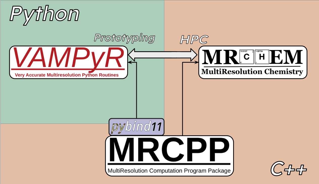
Figure 1: Connections between MRChem, MRCPP and VAMPyR. MRCPP implements a high-performance MRA framework with MWs. It implements the representation of functions and operators as well as fast algorithms for operator application. MRChem implements electronic structure methods and uses MRCPP for the underlying mathematical operations. VAMPyR imports features from MRCPP using Pybind11 and brings intuitive design and easy prototyping through Python. It is used as a Python library can therefore be interfaced other quantum chemistry software. VAMPyR doesn’t include functionality from MRChem, at the current stage. All software packages are available on GitHub, under the MRChemSoft organizationmrc (2023a).

In the architecture of VAMPyR, MRCPP serves as the foundational layer, integrated into Python through Pybind11, as illustrated in Figure 1. This setup enables seamless interoperability between Python and C++, allowing Pybind11 to automatically convert many standard C++ types to their Python equivalents and vice versa. This leads to a more Pythonic and natural interface to the MRCPP codebase.

For the development of VAMPyR, we opted for Pybind11 as our binding framework, chiefly for its robustness, maintainability, and alignment with our development objectives. Pybind11 is a lightweight, header-only library that utilizes modern C++ standards to infer type information, thus streamlining the binding process and enhancing overall code quality.

To facilitate deployment, multiple installation options are available for VAMPyR and MRCPP. The source code for both is openly accessible and distributed under the LGPLv3 license on GitHub, specifically within the MRChemSoft organizationmrc (2023a). For users who prefer a simplified installation procedure, binary packages are also provided through the Conda package manager, which is compatible with various Linux and macOS architecturesmrc (2023b); vam (2023). Each new release triggers an automated build process that uploads the binary packages to the Conda Forge channel on anaconda.org, thereby easing the installation process and incorporating all requisite dependencies. The packages are designed to be compatible with current Python versions, ranging from 3.8 to 3.11. The installation process using Conda is straightforward:

⬇

conda install vampyr -c conda-forge

III.1 Implementation

In MRCPP, C++ template classes and functions are utilized to provide abstraction over the dimensionality of the simulation box. These templates enable the generic implementation of data structures and algorithms for problems in $D$ dimensions. The specialization for 1-, 2-, and 3-dimensional problems is performed at compile-time, thereby eliminating any impact on runtime performance.Vandevoorde, Josuttis, and Gregor (2018)

In Python, native template constructs are absent, presenting a challenge for dimension-specific specialization. In VAMPyR, we emulate MRCPP’s generic approach by implementing dimension-dependent bindings using Pybind11. Specifically, our binding code incorporates template classes and functions similar to those in MRCPP. MRCPP’s 1-, 2-, and 3-dimensional template classes and functions are directly bound to their corresponding dimensions in VAMPyR, as demonstrated in Listing 2. Through this approach, VAMPyR keeps the flexible design of MRCPP, despite Python’s limitations in handling generic datatypes.

Figure 2: Importing dimensional-dependent bindings from VAMPyR.

⬇

from vampyr import vampyr1d

from vampyr import vampyr2d

from vampyr import vampyr3d

While the MultiResolutionAnalysis (see section IV.1) and FunctionTree (see section IV.2) classes in VAMPyR are inherited from MRCPP, there are noteworthy distinctions between the vanilla C++ and the corresponding Python classes. These differences are introduced to enhance the Python version of the MRCPP classes with so call syntactic sugar, which improves the user experience and leads to faster prototyping. Among these enhancements are the overload of various dunder (double underscore, also known as magic) methods that have been added to the classes to extend their functionalities and make them more Pythonic.

These dunder (or magic) methods enable the use of Python’s built-in operators on FunctionTree objects. For instance, the addition (__add__) and multiplication (__mul__) operators allow for the direct use of + and * operators with FunctionTree objects. This allows to write more intuitive code, which is easier to both read and write.

As an example, consider the addition of two FunctionTree objects, which be expressed in natural Python syntax (Listing 3), thanks to the binding code in Listing 4.

Figure 3: Syntax sugar for FunctionTree addition in action.

⬇

f_tree1 = vp.FunctionTree(MRA)

f_tree2 = vp.FunctionTree(MRA)

f_tree_sum = f_tree1 + f_tree2

Figure 4: C++ binding for operator +.

⬇

// allocate new FunctionTree for the output

auto out = std::make_unique<FunctionTree<D>>(inp_a->getMRA());

// arrange input operands in vector of summands

FunctionTreeVector<D> vec;

vec.push_back({1.0, inp_a});

vec.push_back({1.0, inp_b});

// build grid for output value based on summands

build_grid(*out, vec);

// perform summation with no additional refinements

add(-1.0, *out, vec);

// return sum of FunctionTree objects

return out;

The Python code in Listing 3 can be equivalently written in the de-sugared form in Listing 5. Although the Listing 5 is more involved than simply applying an arithmetic operator, it does provide more flexibility and control which might be necessary in some specific applications.

Figure 5: De-sugared syntax for FunctionTree addition using the advanced bindings submodule.

⬇

from vampyr import vampyr3d as vp

\parf_tree1 = vp.FunctionTree(MRA)

f_tree2 = vp.FunctionTree(MRA)

\parf_tree_sum = vp.FunctionTree(mra)

\parvp.advanced.add(-1.0, f_tree_sum, 1.0, f_tree1, 1.0, f_tree2)

IV Mathematics with VAMPyR

In this section we display some of the theoretical concepts discussed in Section II with practical examples using VAMPyR.

IV.1 The MultiResolutionAnalysis Object in VAMPyR

The foundation of VAMPyR’s internal operations is built upon the MultiResolutionAnalysis object. This object encapsulates essential information about the physical space being modeled, along with configurations for the scaling and wavelet basis functions as defined in the theory of MRA (see Section II).

Standard Usage

For users seeking a straightforward implementation, VAMPyR provides a “Standard Usage” option. In this approach, users are only required to specify the box size and polynomial order. The remaining parameters, such as the choice of interpolating polynomials for the scaling basis, are automatically configured by the library. Listing 6 illustrate how to create an MRA object either specifying the start and end points, or the length: the former has length $2L$ whereas the latter starts in $0$ and ends in $L$.

Figure 6: Standard usage of the MRA object.

⬇

# For a unit cell centered at the origin

MRA = vp.MultiResolutionAnalysis(box=[-L,L], order=k)

# For a unit cell with left corner at the origin

MRA = vp.MultiResolutionAnalysis(box=[L], order=k)

Advanced Usage

For users requiring more control over the computational setup, VAMPyR offers an “Advanced Usage” approach. This method allows for the customization of various parameters, including the world box size and the specific type of scaling basis, such as Legendre polynomials. This level of customization grants the user full control over the basis configuration, as demonstrated in Listing 7.

Figure 7: Advanced usage of the MRA object.

⬇

# Construct scaling basis

scaling_basis = InterpolatingBasis(order) # or LegendreBasis(order)

# Define world box

world_box = BoundingBox(scale=0, corner=[x0, y0, z0],

nboxes=[Nx, Ny, Nz], scaling=[a, b, c])

# in 3D, for 1D and 2D replace list of size 3 with list of size 1 or 2

# Construct MRA

MRA = vp.MultiResolutionAnalysis(box=world_box, basis=scaling_basis)

This flexibility allows users to choose the level of interaction with the MRA object based on their specific needs and expertise.

IV.2 Function Projectors

In VAMPyR, functions are represented using a tree-based data structure: the FunctionTree object. This structure naturally arises from the MRA framework outlined in Section II.3.

The Tree

The FunctionTree object consists of interconnected nodes organized hierarchically. The root node represents the entire physical domain, and each non-terminal node or branch begets $2^{d}$ child nodes while connecting to a single parent node. Terminal nodes, or leaves, possess a parent but have no children. Here, $d$ represents the dimensionality of the system. VAMPyR currently supports $d=1,2,3$.

The Node

Each node corresponds to a $d$-dimensional box within the physical domain and encapsulates information about a specific set of scaling and wavelet functions defined therein. Specifically, each node indexed by scale $n$ and translation vector $\mathbf{l}=(l_{1},l_{2},\ldots,l_{d})$ stores $(k+1)^{d}$ scaling coefficients and $(2^{d}-1)(k+1)^{d}$ wavelet coefficients. Here the indices $n$ and $\mathbf{l}$ dictate the node’s spatial size and position, respectively.

IV.3 Scaling and Wavelet projectors in VAMPyR

To facilitate the implementation of function projections into scaling and wavelet spaces, VAMPyR provides the vp.ScalingProjector and vp.WaveletProjector classes. In Listing 8, we define a lambda function f, whose body can be any valid Python expression. This illustrates how to project a function using the vp.ScalingProjector and vp.WaveletProjector classes. Instances P_n and Q_n are created to perform the projection into the scaling and wavelet spaces. The resulting representations, denoted f_n and df_n, are fully described by their mathematical definitions in Equations (7) and (9), respectively.

Figure 8: Function Projection in VAMPyR by Scaling and Wavelet projectors.

⬇

f = lambda x: <analytic function>

P_n = vp.ScalingProjector(MRA, scale=n)

Q_n = vp.WaveletProjector(MRA, scale=n)

f_n = P_n(f)

df_n = Q_n(f)

Figures 9 and 10 provide visual insights into the projection of an exponential (Slater) function, $e^{-a|r|}$, onto different scales. Each figure consists of two subfigures: the left-hand side displays the scaling function space (Figures 9(a) and 10(a)), while the right-hand side illustrates the wavelet function space (Figures 9(b) and 10(b)).

In Figure 9, the projection onto the root scale is far from the target, and the large wavelet part indicates that a representation at a finer scale is mandatory. The vertical lines in both subfigures delineate the physical space spanned by $k+1$ scaling and wavelet functions. In Figure 10, the exponential (Slater) function is projected onto the 4th scale. The representation is now close to its target function: it is however not as sharp as the original exponential (Slater) function, and the wavelet projection indicates that in the cusp region, a finer representation would be required to attain high precision.

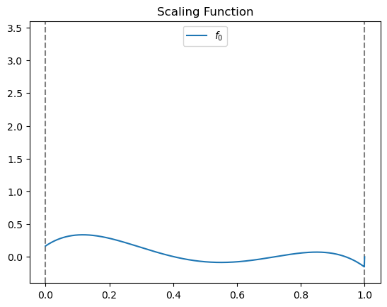
(a)

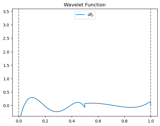
(b)

Figure 9: Projection of a Slater function at root scale. Left: Projection onto scaling function space $V^{0}_{4}$ with vertical lines marking the physical space spanned by $k+1$ scaling functions. Right: Projection onto wavelet function space $W^{0}_{4}$, where vertical lines indicate the physical space spanned by $k+1$ wavelet functions.

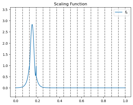
(a)

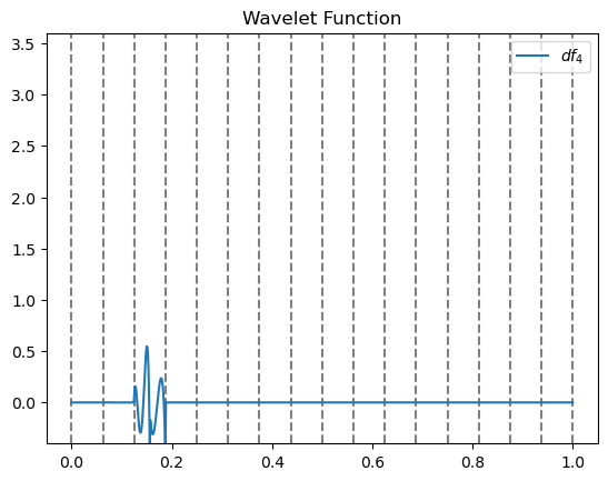
(b)

Figure 10: Projection of a Slater function at the 4th scale. Left: Projection onto scaling function space $V^{4}$, with vertical lines delineating the physical space spanned by $k+1$ scaling functions. Right: Projection onto wavelet function space $W^{4}$, where vertical lines mark the physical space spanned by $k+1$ wavelet functions.

IV.4 Adaptive Projection in VAMPyR

Building on the mathematical framework presented in Section II.4, we cover here the practical aspects of adaptive projection within VAMPyR. Unlike the fixed-scale projection illustrated in Listing 8, adaptive projection makes use of the prec keyword to refine the function’s representation, as shown in Listing 11.

Figure 11: Adaptive Function Projection in VAMPyR.

⬇

P_eps = vp.ScalingProjector(MRA, prec=epsilon)

f_eps = P_eps(f)

The visual comparison in Figure 12 between the adaptive and fixed-scale projections (previously shown in Figures 9 and 10) reveals the power of adaptivity: a representation which is at the same time more compact as well as more precise is achieved. As Figure 12 shows, nodes at finer and finer resolution are created only where it is necessary to represent the sharp features of the function. This strategy is also computationally more efficient as it guarantees that resources are used where and when needed, based on precision requirements.

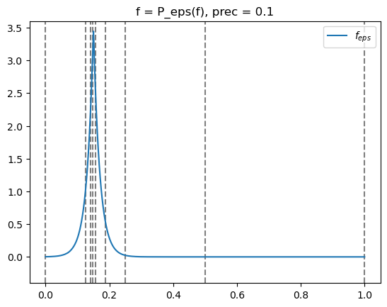
Figure 12: Adaptive projection of the Slater function with prec = $1.0\times 10^{-1}$. The non-uniform vertical lines indicate the physical space spanned by the adaptive basis functions, underscoring the method’s efficiency and precision.

IV.5 Arithmetic Operations in FunctionTrees

In VAMPyR, arithmetic operations on FunctionTree objects are intuitive and flexible. Standard Python operators like $+$, $-$, $*$, $/$, and $**$ are employed for these elementary operations. For an example see Listing 13. where we have examples of usage for both standard arithmetic operations between FunctionTrees and between FunctionTrees and scalars. In these examples, $f$ and $g$ are instances of FunctionTree, and $a$ is a scalar. These operations provide an efficient and user-friendly way to manipulate FunctionTree objects in VAMPyR.

Figure 13: Basic Arithmetic Operations in VAMPyR.

⬇

# Arithmetics with scalars

a_mult_f = a * f # Scalar on the left

f_mult_a = f * a # Scalar on the right

f_div_a = f / a # Division by scalar

f_pow_a = f ** a # Power operator

\par# Arithmetics between FunctionTrees

f_mult_g = f * g # Multiplication operator

f_add_g = f + g # Addition operator

f_sub_g = f - g # Subtraction operator

\par# In-place arithmetics

f *= a # Multiplication with scalar

f *= g # Multiplication with function

f += g # Addition with function

f -= g # Subtraction with function

IV.6 Vectorizing FunctionTrees with NumPy

The integration between the overloaded arithmetic methods in VAMPyR and NumPy’s flexible data structures provides a range of computational advantages. Among these advantages, the support for multi-dimensional arrays, broadcasting, and linear algebra operations stand out. Although NumPy is primarily optimized for integers and floating-point numbers, its data structures can be extended to accommodate custom objects such as FunctionTrees. This capability enables the incorporation of FunctionTrees within NumPy arrays, thus allowing for the full suite of NumPy’s array-oriented computing features. For illustration, consider the example in Listing 14, where we construct a matrix of FunctionTrees within a NumPy array and execute various matrix operations.

Figure 14: Performing matrix operations using function trees in a NumPy array.

⬇

# Creation of a matrix containing function trees

matrix_a = np.array([[a11_tree, a12_tree], [a21_tree, a22_tree]])

matrix_b = np.array([[b11_tree, b12_tree], [b21_tree, b22_tree]])

\par# Performing matrix multiplication

matrix_mul = matrix_a @ matrix_b

\par# Performing addition and subtraction

matrix_sum = matrix_a + matrix_b

matrix_neg = matrix_a - matrix_b

\par# Multiplication by a scalar

matrix_mul_scalar = 2 * matrix_a * matrix_b

\par# Demonstrating broadcasting by adding a single function tree to all elements

matrix_a_bcast_add = matrix_a + single_tree

As demonstrated in Listing 14, the integration between VAMPyR’s FunctionTree objects and NumPy arrays simplifies the implementation of complex mathematical operations. Through NumPy’s multi-dimensional arrays, it is possible to organize and manipulate arrays of function trees efficiently. Broadcasting allows for the addition of a single FunctionTree (or scalar) to an entire array of FunctionTrees. Furthermore, NumPy’s built-in linear algebra functions, such as the matrix multiplication operator @, can be used for matrix operations. This approach improves the readability of the code, as will be seen in Section V.

IV.7 Derivative Operators in VAMPyR

Handling derivatives with MWs is not straightforward: traditional derivative operators are not applicable. However, VAMPyR offers two specialized operators to address this issue, each tailored for specific requirements concerning the continuity of the function and the desired order of the derivative. These methods are based on the works by Alpert et al., giving the ABGVOperator,Alpert et al. (2002) and Anderson et al., leading to the BSOperator.Anderson et al. (2019a)

Both the ABGVOperator and the BSOperator apply the operators following the NS form as described in Subsection II.5, allowing for efficient and accurate calculations:

ABGVOperator

Designed for piece-wise continuous functions, this operator provides a weak formulation for first-order derivatives. It is primarily suitable for handling first-order derivatives and offers a balance between accuracy and computational efficiency. Usage is demonstrated in Listing 15.

BSOperator

This operator is more versatile but it works best for smooth continuous functions. It accommodates higher-order derivatives by transforming the function onto a B-spline basis before differentiation. See Listing 16 for a practical example.

Figure 15: First-order derivatives using ABGVOperator.

⬇

D = vp.ABGVOperator(MRA)

\par# x, y, z derivatives using ABGVOperator

f_x = D(f, 0)

f_y = D(f, 1)

f_z = D(f, 2)

Figure 16: First- and second-order derivatives using BSOperator.

⬇

D1 = vp.BSOperator(MRA, 1) # First-order derivative operator

D2 = vp.BSOperator(MRA, 2) # Second-order derivative operator

\par# First-order derivatives

f_x = D1(f, 0)

f_y = D1(f, 1)

f_z = D1(f, 2)

\par# Second-order derivatives

f_xx = D2(f, 0)

f_yy = D2(f, 1)

f_zz = D2(f, 2)

IV.8 Convolution Operators in VAMPyR

Convolution operators are essential tools for solving integral forms of key equations in Quantum Chemistry, such as the integral formulation of the Hartree–Fock (HF) and Kohn–Sham (KS) equations or the Poisson equation used in self-consistent reaction field (SCRF) models. Both equations can be recast from the more familiar differential form, to an equivalent integral form by making use of the Bound–State Helmholtz (BSH) kernel (see Appendix A) and the Poisson kernel. The key step in both problems is the convolution of the corresponding Green’s function kernel with a test function:

$$g(\mathbf{x})=\int K(\mathbf{x},\mathbf{y})f(\mathbf{y})\text{d}\mathbf{y}.$$ (19)

The two kernels are numerically implemented in the MRCPP library and available in VAMPyR. They are constructed as a sum of Gaussians which represents the numerical quadrature of the integral of a superexponentially decaying functionFrediani et al. (2013) which depends on the distance $d=|\mathbf{x}-\mathbf{y}|$.

$$K(\mathbf{x},\mathbf{y})=\frac{e^{-\mu|\mathbf{x}-\mathbf{y}|}}{|\mathbf{x}-\mathbf{y}|}\approx\sum_{i=1}^{M}\alpha_{i}\exp(-\beta_{i}|\mathbf{x}-\mathbf{y}|^{2}),$$ (20)

In the expression above, $\mu=0$ yields the Poisson kernel, and $\mu>0$ corresponds to the bound-state Helmholtz kernel.

Figure 17: Creating and applying Poisson and Helmholtz operators in VAMPyR.

⬇

P_oper = vp.PoissonOperator(mra, prec)

H_oper = vp.HelmholtzOperator(mra, mu, prec)

\parg_tree = P_oper(f_tree)

g_tree = H_oper(f_tree)

A more general method for constructing convolution operators based on Gaussian expansions is also available in VAMPyR. This approach is documented with an example in Listing 18 and an unusual application is illustrated in Figure 19 by blurring an image with a Gaussian convolution kernel, although VAMPyR is not generally optimized for such tasks.

Figure 18: Construction of a Custom Convolution Operator in VAMPyR.

⬇

# Create a 1D GaussExp object, serving as a container for Gaussians

kernel = vp1.GaussExp()

# Append a Gaussian function to the kernel

kernel.append(vp1.GaussFunc(beta, alpha))

# Construct the convolution operator

T = vp.ConvolutionOperator(mra, kernel, prec)

# Apply the operator to a function tree

g_tree = T(f_tree)

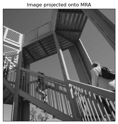
(a) Original image projected onto the Multi-Resolution Analysis (MRA).

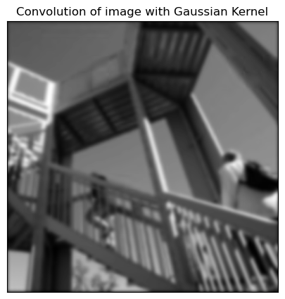
(b) Resulting image after performing convolution with a Gaussian Kernel, leading to smoothing or blurring of the original image.

Figure 19: Illustration of convolution process in VAMPyR.

V Four little pieces of quantum chemistry

One of the main technical challenges of quantum chemistry is the large gap between the equations describing the physical nature of the system and their practical realization in a working code. This gap arises because the equations in their original form are in general too complicated to be solved. To achieve equations which have a manageable computational cost, it has so far been necessary to make use of representations which on the one hand lead to practical numerical implementation, but on the other hand obfuscate the original physical equations.

We will here present four little pieces of quantum chemistry where we show how the MW representation of functions and operators in MRCPP and the simple Python interface provided by VAMPyR can close this semantic gap.

For each of the four examples presented, we will highlight how VAMPyR has been employed to obtain working implementations that closely resembles the theoretical framework. The underlying equations will here be presented briefly to highlight their correspondence with the code. We refer to separate appendices, or previously published work, for a more in-depth exposition of the theory.

All examples are available as Jupyter notebooks in a separate GitHub repositoryvam (2024b), openly accessible under the CC-BY-4.0 license.

V.1 The Hartree–Fock Equations

The Hartree-Fock equationsJensen (2017) can be concisely written as:

$$\hat{F}\varphi_{i}=\sum_{j}F_{ij}\varphi_{j}$$ (21)

where $\hat{F}$ is the Fock operator, $\varphi_{i}$ is an occupied orbital and $F_{ij}$ are the Fock matrix elements in the basis of the occupied orbitals.

Traditionally, a basis-set representation is introduced and most of the successive discussion regards methods to achieve a good performance and a sufficient precision. A MW representation avoids this complication and solves the equations directly. As shown in Appendix A, this is achieved by recasting the problem as an integral equation:

$$\tilde{\varphi}_{i}^{n+1}=-2\hat{G}^{\mu^{n}_{i}}\left[\left(V_{N}+2J^{n}-K^{n}\right)\varphi_{i}^{n}-\sum_{j\neq i}F^{n}_{ij}\varphi_{j}^{n}\right]$$ (22)

In the above equation, $\hat{G}^{\mu_{i}^{n}}$ is the bound-state Helmholtz operator, $V_{N}$, $J$ and $K$ are the nuclear, Coulomb and exchange operator, respectively and we have restricted ourselves to closed-shell systems. $i$ is the orbital index and $n$ represents the iteration index and is displayed for all quantities that are iteration-dependent. The resulting orbitals $\tilde{\varphi}_{i}$ are not normalized (here indicated with a $\tilde{}$ superscript) and an orthonormalization step must then be performed. The complete algorithm can be found in the accompanying Python notebook vam (2024b) and includes a Löwdin orthogonalization of the orbitals, ensuring the desired orthogonality condition. We base our implementation on these equations. The Self–Consistent Field (SCF) equations (22) are implemented in Python, as demonstrated in Listing 20. Thanks to the VAMPyR interface the code is now directly corresponding to the mathematical formalism without any intermediate representation.

Figure 20: Python implementation of the SCF equation.

⬇

VPhi = V_nuc(Phi_n) + 2*J_n(Phi_n) - K_n(Phi_n)

Phi_np1 = -2*G(VPhi + (Lambda_n - F_n) @ Phi_n)

To achieve an even more compact structure, the set of orbitals can be collected in a NumPy vector. This requires that the implementation of operators in the code accepts a vector of orbitals as input. The operators V_nuc, J_n, and K_n (defined in equations (37), (38), and (39), respectively) are implemented in a vectorized manner using NumPy. For example, the CouloumbOperator class is presented in Listing 21.

Figure 21: Python implementation of the Couloumb operator.

⬇

class CouloumbOperator():

def __init__(self, mra, Psi, prec):

self.mra = mra

self.Psi = Psi

self.prec = prec

self.poisson = vp.PoissonOperator(mra=mra, prec=self.prec)

self.potential = None

self.setup()

def setup(self):

rho = self.Psi[0]**2

for i in range(1, len(self.Psi)):

rho += self.Psi[i]**2

rho.crop(self.prec)

self.potential = (4.0*np.pi)*self.poisson(rho).crop(self.prec)

def __call__(self, Phi):

return np.array([(self.potential*phi).crop(self.prec) for phi in Phi])

V.2 Continuum solvation

A very common approach to including solvent effects in a quantum chemistry calculation is to consider the molecule immersed in a dielectric continuum. The governing equation is the generalized Poisson equation (GPE):

$$\nabla\cdot\left[\epsilon(\mathbf{r})\nabla V(\mathbf{r})\right]=-4\pi\rho(\mathbf{r})$$ (23)

where $V$ is the electrostatic potential, $\rho$ is the charge distribution of the molecule and $\epsilon$ is the (position-dependent) permittivity of the dielectric. The practical solution of the equation depends on how $\epsilon$ is parametrized. Traditionally, a cavity boundary is defined and the permittivity is a step function of the cavity: $\epsilon_{i}=1$ inside of it and $\epsilon_{o}=\epsilon_{s}$ outside, where $\epsilon_{s}$ is the bulk permittivity of the solvent. This parametrization leads to an equivalent boundary integral equation, solved with a suitable boundary element method.Tomasi, Mennucci, and Cammi (2005) The main advantage of the approach is transferring the problem from the (infinite) 3-dimensional space to the (finite) cavity surface. The main disadvantage is a less physical parametrization of the model, due to the presence of the sharp boundary.

Using MWs, Equation 23 can instead be solved directly, without assumptions on the functional form of $\epsilon$. The main working equation is the application of the Poisson operator $\hat{P}$ to the effective charge density $\rho_{\mathrm{eff}}(\mathbf{x})$ and the surface polarization $\gamma(\mathbf{x})$:

$$V(\mathbf{x})=\hat{P}\left[\rho_{\mathrm{eff}}(\mathbf{x})+\gamma(\mathbf{x})\right],$$ (24)

where the effective density $\rho_{\mathrm{eff}}$ and the surface polarization $\gamma(\mathbf{x})$ are defined respectively as:

$$\rho_{eff}(\mathbf{x}) =\frac{\rho(\mathbf{x})}{\varepsilon(\mathbf{x})}$$ (25)

$$\gamma(\mathbf{x}) =\frac{\nabla\log\epsilon\cdot\nabla V}{4\pi}.$$ (26)

The surface polarization depends on the potential, which implies that the equation must be solved iteratively.

The equations above are easily represented in a MW framework and each of them can be written as a single line of code with VAMPyR. This is shown in Listing 22. The model is extensively discussed in a previous paperGerez S. et al. (2023) where a thorough study of theory and implementation was presented. The example in Listing 22 shows how continuum solvation has been implemented using VAMPyR. Here we have assumed we already have a projected permittivity function and the total solute density function together with a suitable mra and a function that computes $\gamma$ called computeGamma.

The solvation energy $E_{R}$ is finally computed from the reaction potential $V_{R}=V-\int d\mathbf{r}^{\prime}\frac{\rho(\mathbf{r}^{\prime})}{|\mathbf{r}-\mathbf{r}^{\prime}|}$, and the solute charge density $\rho$:

$$E_{R}=\frac{1}{2}\int d\mathbf{x}V_{R}(\mathbf{x})\rho(\mathbf{x}).$$ (27)

Figure 22: Python implementation of PCM in VAMPyR.

⬇

# Initialize the poisson operator

P = vp.PoissonOperator(mra=mra, prec=1.0e-5)

# Solve the standard Poisson equation

V_vac = P(4*pi*density)

# Compute the initial gamma_s

gamma_s = computeGamma(V_vac)

# Construct effective density rho_eff

rho_eff = (4 * np.pi) * ((density * (permittivity)**(-1)) - density)

# Compute the initial reaction potential

V_R = P(rho_eff + gamma_s)

# Solve the GPE by iteration

for i in range(100):

V = V_vac + V_R

gamma_s = computeGamma(V, permittivity)

V_R_np1 = P(rho_eff + gamma_s)

dV_R_n = V_R_np1 - V_R

update = dV_R_n.norm()

V_R = V_R_np1.deepCopy()

if (abs(update) <= 1.0e-5):

break

# compute the final energy and finish.

E_R = (1/2)*vp.dot(V_R, rho)

V.3 Implementation of 4-component Dirac Equation for one-electron

Lately we have made use of VAMPyR to extend our work towards the relativistic domain. As such VAMPyR has been used for a range of proof-of-principle calculations which all stem from the Dirac equation.Tantardini et al. (2024); Tantardini, Di Remigio Eikås, and Frediani (2023) It is well known that the level of complexity required to deal with the Dirac equation increases significantly: the scalar non-relativistic eigenvalue problem, dealing generally with real-valued functions, becomes a 4-component problem involving complex functions:

$$\begin{pmatrix}(V+mc^{2}-\epsilon)&c(\mathbf{\sigma}\cdot\mathbf{p})\\ c(\mathbf{\sigma}\cdot\mathbf{p})&(V-\epsilon-mc^{2})\end{pmatrix}\begin{pmatrix}\psi^{\mathrm{L}}\\ \psi^{\mathrm{S}}\end{pmatrix}=0$$ (28)

where $V$ is the external potential, $\epsilon$ is the energy eigenvalue, $c$ is the speed of light, $\mathbf{p}$ is the momentum operator and $\sigma$ is the vector collecting the three Pauli matrices. As shown by Blackledge and BabajanovBlackledge and Babajanov (2013) and later exploited by Anderson et al.Anderson et al. (2019b), the Dirac equation can also be reformulated as an integral equation as:

$$\begin{pmatrix}\psi^{\mathrm{L}}\\ \psi^{\mathrm{S}}\end{pmatrix}=\frac{-1}{2mc^{2}}\begin{pmatrix}(\epsilon+mc^{2})&c(\mathbf{\sigma}\cdot\mathbf{p})\\ c(\mathbf{\sigma}\cdot\mathbf{p})&(\epsilon-mc^{2})\end{pmatrix}\hat{G}^{\mu}\left[V\begin{pmatrix}\psi^{\mathrm{L}}\\ \psi^{\mathrm{S}}\end{pmatrix}\right]$$ (29)

where $\hat{G}^{\mu}$ is the BSH kernel as in the non relativistic case (see Section IV.8), and $\mu=\sqrt{\frac{m^{2}c^{4}-\epsilon}{mc^{2}}}$.

The above integral equation can be solved iteratively as in the non-relativistic case and the algorithm is thus very similar to the non-relativistic case. The main difference is that the infrastructure required to deal with 4-component spinors needs to be implemented. Our design is built essentially on two Python classes: one to deal with complex functions (a single component of a spinor is a complex function) and another one to deal with the four components. Thanks to VAMPyR, these classes are easy to implement and use, for the most part overloading dunder operators.

The Listing 23 shows a portion of the class implementation for the 4-component Spinor. The objects are made callable and work as NumPy arrays. Each component is itself a complex function object (defined in a separate class). Some dunder methods are shown and the methods to perform the operation $c(\alpha\cdot\mathbf{p})\psi$ are also reported.

Figure 23: Excerpt of the 4-component spinor class.

⬇

class Spinor:

"""Four components orbital."""

mra = None

light_speed = -1.0

comp_dict = {’La’: 0, ’Lb’: 1, ’Sa’: 2, ’Sb’: 3}

def __init__(self):

self.comp_array = np.array([cf.complex_fcn(),

cf.complex_fcn(),

cf.complex_fcn(),

cf.complex_fcn()])

def __getitem__(self, key):

return self.comp_array[self.comp_dict[key]]

def __setitem__(self, key, val):

self.comp_array[self.comp_dict[key]] = val

def __len__(self):

return 4

def __add__(self, other):

output = orbital4c()

output.comp_array = self.comp_array + other.comp_array

return output

def __call__(self, position):

return [x(position) for x in self.comp_array]

def __rmul__(self, factor):

output = orbital4c()

output.comp_array = factor * self.comp_array

return output

def alpha(self, direction, prec):

out_orb = orbital4c()

alpha_order = np.array([[3, 2, 1, 0],

[3, 2, 1, 0],

[2, 3, 0, 1]])

alpha_coeff = np.array([[ 1, 1, 1, 1],

[-1j, 1j, -1j, 1j],

[ 1, -1, 1, -1]])

for idx in range(4):

coeff = alpha_coeff[direction][idx]

comp = alpha_order[direction][idx]

out_orb.comp_array[idx] = coeff * self.comp_array[comp]

out_orb.comp_array[idx].crop(prec)

return out_orb

def alpha_p(self, prec, der = "ABGV"):

out_orb = orbital4c()

orb_grad = self.gradient(der)

apx = orb_grad[0].alpha(0, prec)

apy = orb_grad[1].alpha(1, prec)

apz = orb_grad[2].alpha(2, prec)

result = -1j * (apx + apy + apz)

result.cropLargeSmall(prec)

return result

With the Spinor class implementation at hand, the iterative scheme to converge the Hydrogen atom is easily implemented:

Figure 24: Iterative solution of the Dirac equation.

⬇

while orbital_error > prec:

hd_psi = orb.apply_dirac_hamiltonian(spinor_H, prec, der = default_der)

v_psi = orb.apply_potential(-1.0, V_tree, spinor_H, prec)

add_psi = hd_psi + v_psi

energy = (spinor_H.dot(add_psi)).real

mu = orb.calc_dirac_mu(energy, light_speed)

tmp = orb.apply_helmholtz(v_psi, mu, prec)

tmp.crop(prec/10)

new_orbital = orb.apply_dirac_hamiltonian(tmp, prec, energy, der = default_der)

new_orbital.crop(prec/10)

new_orbital.normalize()

delta_psi = new_orbital - spinor_H

orbital_error = (delta_psi.dot(delta_psi)).real

print(’Error’,orbital_error, imag, flush = True)

spinor_H = new_orbital

First the energy is computed in order to obtain the parameter $\mu$, then comes the convolution of $V\psi$ with the Helmholtz kernel $\hat{G}^{\mu}$, and finally the Dirac Hamiltonian plus the energy $h_{D}+\epsilon$ is applied to the convolution. The iteration is repeated until the norm of the spinor update is below the requested threshold. At the end of the iteration the energy must be computed once more (not reported in the listing).

V.4 Time-dependent Schrödinger equation

The MWs framework can successfully be employed for real-time simulations of a wavepacket by directly integrating the time-dependent Schrödinger equation:

$$i\partial_{t}\Psi=\left(\hat{T}+\hat{V}\right)\Psi,$$ (30)

where the potential $\hat{V}$ may be time-dependent. For simplicity we consider here a time-independent potential and a one-dimensional problem: $V=V(x)$ and $\Psi=\Psi(x,t)$ with $x,t\in\mathbb{R},$ and we assume that the initial conditions are given as $\Psi(x,0)=\Psi_{0}(x)$. The standard numerical treatment of (30) is to choose a small time step $t>0$ and construct the time evolution operator on the interval $[0,t]$. By applying it iteratively, the solution at any finite time can in principle be obtained. The wave propagation can be expressed as

$$\Psi(t)=\exp\left(-it\left(\hat{T}+\hat{V}\right)\right)\Psi_{0},$$ (31)

where we used the fact that the potential is time-independent. We proceed by splitting the propagator in the kinetic $\exp\left(-it\hat{T}\right)$ and potential $\exp\left(-it\hat{V}\right)$ parts. The former is a multiplicative operator in momentum space, whereas the latter is a multiplicative operator in real space. This separation is not exact, because $\hat{T}$ and $\hat{V}$ do not commute. The resulting operator has an error of order $\mathcal{O}\left(t^{2}\right)$:

$$\exp\left(-it\left(\hat{T}+\hat{V}\right)\right)=\exp\left(-it\hat{T}\right)\exp\left(-it\hat{V}\right)+\mathcal{O}\left(t^{2}\right).$$ (32)

This simple splitting is too rough for practical applications, therefore we make use of the following fourth order scheme Chin and Chen (2001)

$$e^{At+Bt}=\exp\left(\frac{t}{6}B\right)\exp\left(\frac{t}{2}A\right)\exp\left(\frac{2t}{3}\widetilde{B}\right)\exp\left(\frac{t}{2}A\right)\exp\left(\frac{t}{6}B\right)+\mathcal{O}\left(t^{5}\right),$$ (33)

where

$$\widetilde{B}=B+\frac{t^{2}}{48}[B,[A,B]].$$ (34)

With $A=-i\hat{T}$ and $B=-i\hat{V}$, $\widetilde{B}$ becomes a multiplicative operator containing the potential gradient $\partial_{x}V(x)$. Remarkably, this high order scheme requires only two applications of the free-particle semigroup operator $\exp\left(-it\hat{T}/2\right)$ per time step. For an example of the implementation see Listing 25.

Figure 25: ChinChen implementation.

⬇

class ChinChenA(object):

def __init__(self, expA, expB, exp_tildeB):

self.expA = expA

self.expB = expB

self.exp_tildeB = exp_tildeB

def __call__(self, u):

u = self.expB(u) # 1/6*dt

u = self.expA(u) # 1/2*dt

u = self.exp_tildeB(u) # 2/3*dt

u = self.expA(u) # 1/2*dt

u = self.expB(u) # 1/6*dt

return u

Complex algebra is not supported natively in VAMPyR, therefore we represent complex exponential operators as follows

$$\exp\left(-i\widehat{H}t\right)=\begin{pmatrix}\cos\widehat{H}t&\sin\widehat{H}t\\ -\sin\widehat{H}t&\cos\widehat{H}t\end{pmatrix},\quad\mbox{operating on vector-functions }\Psi(t)=\begin{pmatrix}u(t)\\ v(t)\end{pmatrix}$$ (35)

where self-adjoint $\widehat{H}$ stands for either the kinetic energy $-\partial_{x}^{2}$, or the potential $V(x)$ or the full Hamiltonian $-\partial_{x}^{2}+V(x)$. The implementation is shown in Listing 26.

Figure 26: Unitary exponent group

⬇

class UnitaryExponentGroup(object):

def __init__(self, real, imag):

self.real = real

self.imag = imag

def __call__(self, psi):

u = psi[0]

v = psi[1]

res0 = self.real(u) - self.imag(v)

res1 = self.imag(u) + self.real(v)

return np.array([ res0, res1 ])

As a worked-out example, we show a simulation of the time evolution of a Gaussian wave packet $\Psi(x,t)$ in harmonic potential $V(x)$:

$$\Psi_{0}(x)=\Psi(x,t=0)=\left(\frac{1}{2\pi\sigma^{2}}\right)^{1/4}\exp\left(-\frac{(x-x_{0})^{2}}{4\sigma^{2}}\right),\qquad V(x)=V_{0}(x-x_{1})^{2}.$$

It is well known that the density $\left|\Psi(t)\right|^{2}$ oscillates in the harmonic potential with the period $\tau=\pi/\sqrt{V_{0}}.$ More precisely, $\Psi\left(\tau\right)=-\Psi_{0}.$ This can immediately be seen taking into account that the eigenvalues for the Hamiltonian are $\sqrt{V_{0}}(2n+1).$ We take $x_{0}=0.3$, $\sigma=0.04$ and $x_{1}=0.5$, $V_{0}=25000$. The parameters are chosen in such a way that the solution stays localized mainly on the $[0,1]$ interval. Note that the $\widetilde{B}$ operator simplifies to

$$\widetilde{B}=-i\widetilde{V}=-iV+\frac{it^{2}}{24}(\partial_{x}V)^{2}=-i\widetilde{V}_{0}(x-x_{0})^{2},\quad\mbox{where }\widetilde{V}_{0}=V_{0}-\frac{(tV_{0})^{2}}{6},$$

.

In Listing 27 we define all the necessary operators and initialize Scheme (33). The numerical integration of the time evolution is performed in Listing 28. Figure 29 shows the result of the simulation: the oscillation movement of the density $\left|\Psi(t)\right|^{2}$ and the difference between the numerical and exact solution at the time moment $t=\tau.$

Figure 27: Preparation to implementation of time evolution in VAMPyR.

⬇

# Define parameters, final time moment and time step

x0 = 0.3

sigma = 0.04

x1 = 0.5

V0 = 25000

N = 20

t_period = np.pi / np.sqrt(V0)

time_step = t_period / N

# Set the precision and make the MRA

precision = 1.0e-5

finest_scale = 9

mra = vp1.MultiResolutionAnalysis(vp1.BoundingBox(0), LegendreBasis(5))

# Make the scaling projector

P = vp1.ScalingProjector(mra, prec = precision)

# Define the harmonic potential with its scheme modification

def V(x):

return V0 * (x[0] - x1)**2

def tilde_V(x):

A = V0 - ( time_step * V0 )**2 / 6.0

return A * (x[0] - x1)**2

# Define the iteration procedure

iteratorA = ChinChenA(

expA = create_unitary_kinetic_operator(mra, precision, time_step / 2, finest_scale),

expB = create_unitary_potential_operator(P, V, time_step / 6),

exp_tildeB = create_unitary_potential_operator(P, tilde_V, 2 * time_step / 3)

)

Figure 28: Time evolution simulation in VAMPyR.

⬇

# Define the initial wave function

psi0 = vp1.GaussFunc(

beta = 1.0 / (4 * sigma**2), alpha = (2 * np.pi * sigma**2)**(-1/4), position = [x0]

)

psi0 = np.array([ P(psi0), vp1.FunctionTree(mra).setZero() ])

# Solve the initial value problem

psiA = psi0

for n in range(N):

psiA = iteratorA(psiA)

# Find error at t = period

per_errorA = psiA + psi0

print( f"L2-norm of real part error: {per_errorA[0].norm()}" )

print( f"L2-norm of imaginary part error: {per_errorA[1].norm()}" )

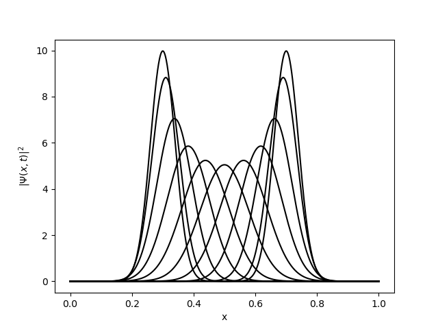
(a) Density evolution in the harmonic potential.

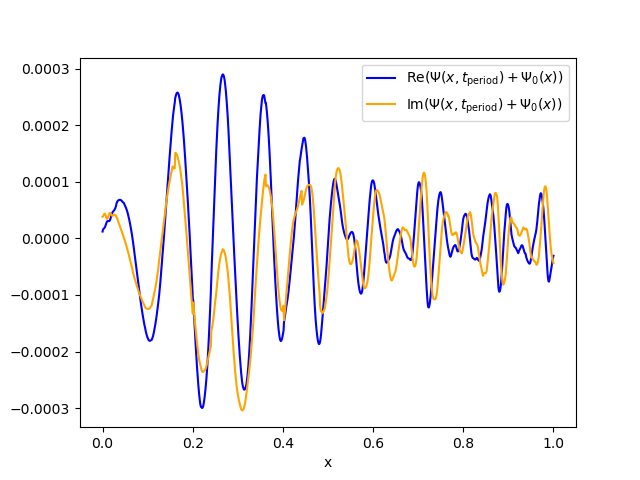
(b) The difference between the numerical and exact solution.

Figure 29: Simulation of (30) in VAMPyR.

VI Interoperability with other packages

One of the main benefits of introducing a Python interface is the seamless interoperability it offers with a number of other packages. This not only simplifies the usage of the package but also enhances its capabilities by allowing the integration of features provided by other packages. In this section, we will explore some potential applications of this interoperability, showcasing how VAMPyR can interact with other packages to perform tasks that may otherwise be computationally demanding or require a more complex implementation.

As an example, the SCF solver implemented in VAMPyR, though fully general, encounters practical limitations with more complex molecular systems. One primary challenge is the selection of an appropriate initial guess for the orbitals; a poor choice can severely impact the convergence rate and even result in a failure to converge. The first step beyond the HF approximation might be to incorporate exchange and correlation density functionals, which, while beneficial, can be tedious to implement.

Here is where interoperability steps in. We can leverage the capabilities of different Python packages to address these issues. We will walk through examples demonstrating how VAMPyR can:

• Use VeloxChemRinkevicius et al. (2020) to generate an initial guess for a SCF, speeding up the process and increasing the chance of successful convergence.

• Use VAMPyR and VeloxChem to compute a potential energy surface grid, effectively utilizing computational resources.

• Perform stability analysis on Density Functional Theory (DFT) functionals from Libxc,Lehtola et al. (2018).

VI.1 Generating an Initial Guess with VeloxChem

Here, we illustrate how to generate an initial guess using VeloxChem that can be imported into VAMPyR. Reconstructing the Molecular Orbitals (or electron density) from the AO basis set using the MO (or density) matrix is a rather complex task, especially if the basis contains high angular momentum functions. We thus want to make use of VeloxChem own internal evaluator for these objects, and wrap a simple function around it which can be projected onto the MW basis using a ScalingProjector. In principle, any $\mathbb{R}^{3}\rightarrow\mathbb{R}$ function can be projected in this way, so we just have to define a function that takes as argument a point in real-space, runs it through VeloxChem internal AO evaluator code, and returns the function value of a given MO at that point.

First, we set up and run the SCF calculation with VeloxChem:

⬇

# Read molecule and basis

molecule = vlx.Molecule.read_str(mol_str)

basis = vlx.MolecularBasis.read(molecule, "PCSEG-1")

# Make SCF and run driver

scf_drv = vlx.ScfRestrictedDriver()

scf_results = scf_drv.compute(molecule, basis)

# Make a visualization driver that can be used to evaluate orbitals.

vis_drv = vlx.VisualizationDriver()

# Get the MO coefficients

mol_orbs = scf_drv.mol_orbs

We can define a function that returns the value of the MO at a given point in space. This function will be used for projecting onto an MRA in VAMPyR:

⬇

# Define a function to get the MOs, this can be projected onto an MRA by vampyr

def mo_i(mol_orbs, r):

R = np.array([r])

return vis_drv.get_mo(R, molecule, basis, mol_orbs, i, "alpha")[0]

Finally, we use a projector from VAMPyR to project the MOs from VeloxChem onto an MRA, generating a list of FunctionTrees for the initial guess:

⬇

# This can now be imported into vampyr as:

P_eps = vp.ScalingProjector(mra, prec)

Phi_0 = [P_eps(mo_i) for i in range(nr_orbs)]

In the last step, we loop over the desired number of orbitals, project each one onto the MRA, and store the result in Phi_0. This list of FunctionTrees represents an approximation to the molecular orbitals of the system, and serves as an excellent initial guess for the SCF procedure in VAMPyR.

VI.2 Calculate a potential energy surface with VeloxChem and VAMPyR

A Potential Energy Surface (PES) can be computed as a series of single point energy calculations while varying one (or more) bond distance(s) in a molecule. We will here use VAMPyR’s adaptive function projector as a driver for computing the PES of the Hydrogen molecule using VeloxChem’s single-point Hartree–Fock evaluator. We define a Python function, pes(r), that computes the energy for two Hydrogen atoms given the bond distance as input:

⬇

def pes(r):

mol_str = f"""

H 0.0 0.0000 -0.2

H 0.0 0.0000 {r[0]}

"""

molecule = vlx.Molecule.read_str(mol_str)

basis = vlx.MolecularBasis.read(molecule, "PCSEG-1")

\parscf_drv = vlx.ScfUnrestrictedDriver()

scf_results = scf_drv.compute(molecule, basis)

return scf_drv.scf_energy

The function above computes the energy of a Hydrogen molecule as a function of the bond distance (the 0.2 offset is to avoid the singularity at $r=0$), by performing an SCF calculation at the given geometry. Being a $\mathbb{R}\rightarrow\mathbb{R}$ mapping, it can be projected on a 1D MRA using VAMPyR.

⬇

mra = vp.MultiResolutionAnalysis(box=[0, 10], order=1)

P_eps = vp.ScalingProjector(mra, prec=1.0e-3)

pes_tree = P_eps(pes)

The adaptive projector will automatically sample the pes(r) function in appropriate points in order to produce a smooth surface. The potential energy surface obtained in this manner can be visualized, as shown in Figure 30.

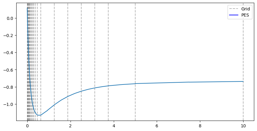
Figure 30: Potential energy surface calculated using VeloxChem and VAMPyR. The grid lines represent the adaptive MRA grid, from which the PES is interpolated.

The vertical lines in Figure 30 represent the adaptive MRA grid, and the potential energy surface depicted is interpolated from this grid rather than computed directly at each point. The adaptive algorithm focuses computational resources where needed to achieve the desired precision. Further efficiency gains could be achieved realizing that high precision is only required for region of low potential energy. This has not been exploited in the above example.

VI.3 Numerical Stability Analysis using VAMPyR and Pylibxc

Inspired by the paper by Lehtola and Marques,Lehtola and Marques (2022) we investigate the numerical stability of density functional approximations (DFAs) lda-c-vwn and lda-c-gk72, with VAMPyR and Pylibxc. The choice of these DFAs is due to their contrasting numerical stability, making them interesting subjects for our analysis. The lda-c-gk72, developed by Gordon and Kim in 1972, was known for its problematic convergence while the lda-c-vwn (Vosko, Wilk, and Nusair functional) was noted for its numerical stability. Our objective is to verify these claims, illustrating the potential of VAMPyR as numerical analysis tool.

Firstly, we initialize a Neon atom and calculate the self-consistent field (SCF) using VeloxChem:

⬇

def init_molecule_and_scf(mol_str, basis_set="PCSEG-1"):

molecule = vlx.Molecule.read_str(mol_str)

basis = vlx.MolecularBasis.read(molecule, basis_set)

scf_drv = vlx.ScfRestrictedDriver()

scf_results = scf_drv.compute(molecule, basis)

return molecule, basis, scf_drv.density

Next, we calculate the density and project it onto a Multi-Resolution Analysis (MRA) grid:

⬇

def calc_density(r, molecule, basis, mol_orbs, vis_drv):

R = np.array([r])

rho_a = vis_drv.get_density(R, molecule, basis, mol_orbs, "alpha")[0] +

rho_b = vis_drv.get_density(R, molecule, basis, mol_orbs, "beta")[0]

return rho_a + rho_b

\parrho = P_eps(lambda r: calc_density(r, molecule, basis, mol_orbs, vis_drv))

Subsequently, we use Pylibxc to define the chosen DFA functionals:

⬇

func_c = xc.LibXCFunctional("lda_c_gk72" or "lda_c_vwn", "unpolarized")

def f_e(n):

c = func_c.compute({"rho": n})["zk"]

return n * (c)

F_e = vp.FunctionMap(f_e, precision)

Following this, an exchange potential is generated. We iteratively refine the grid based on precision, one scale at a time, until no new nodes are created:

⬇

v_x = vp.FunctionTree(mra)

nNodes = v_x.nNodes()

while nNodes > 0:

vp.advanced.clear_grid(v_x)

vp.advanced.map(-1.0, v_x, rho, f_e)

print(f"nodes : {v_x.nNodes()} norm : {v_x.norm()}", flush=True)

nNodes = vp.advanced.refine_grid(v_x, precision)

Observing the output for each DFA, we note that the number of nodes converges to a finite value for the chosen precision in case of the lda_c_vwn functional. For the lda_c_gk72 functional the number of nodes grows exponentially before the requated precision is reached. Looking at the wavelet norm, we notice that we are i still fa r from a converged result. In this example we employed a rather high precision ($\epsilon=10^{-8}$).

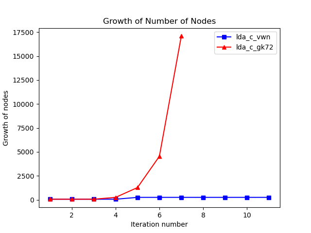
Figure 31: Comparison of node growth between the lda-c-vwn and lda-c-gk72 DFAs. The plot illustrates the sharp contrast in the convergence behavior, with lda-c-vwn showing a stable, linear growth, and lda-c-gk72 displaying an exponential growth.

VII Summary

Multiresolution analysis is a relatively new tool in quantum chemistry, compared to traditional methods based on atomic orbitals. Its main advantages are the possibility to reach any predefined arbitrary precision (the only limits are dictated by the machine precision and the available memory), and a numerical implementation which stays close to the theoretical formalism. VAMPyR has been designed to capitalize on these two aspects, and at the same time enable fast code development for prototype applications.

We have employed VAMPyR to test new ideas and methods, and to create interfaces with existing codes. In the first category, we have here shown a simple SCF optimization, a continuum solvation model, the solution of the Dirac equation for one electron and the application of the time evolution operator. In the second, we illustrated how to import a starting guess for the orbitals, the plotting of a PES, a numerical analysis of two density functionals. For all the above examples we have provided extracts of the code which show how VAMPyR is used. The complete set of working examples illustrated in Section V has been collected in an openly accessible GitHub repositoryvam (2024b), under the CC-BY-4.0 license.

Appendix A The Self Consistent Field equations of Hartree–Fock and Density Functional Theory

The starting point of most Quantum Chemistry calculations involve one Slater determinant, because it automatically accounts for the Pauli exclusion principle and allows to express quantities in a sum of orbital contributions. In particular, the energy expression for a Slater determinant $\Psi$ in atomic units is given by:

$$E[\Psi]=\sum_{i}\braket{\psi_{i}}{\hat{h}}{\psi_{i}}+\frac{1}{2}\sum_{i,j}\braket{\psi_{i}}{\hat{J}_{j}-\hat{K}_{j}}{\psi_{j}}$$ (36)

Here, $\hat{h}$ is the one-electron Hamiltonian:

$$\hat{h}=\hat{T}+\hat{V}_{N}=-\frac{1}{2}\nabla^{2}-\sum_{I}\left(\frac{Z_{I}}{|r-R_{I}|}\right),$$ (37)

with $\hat{T}$ the kinetic energy operator and $\hat{V}_{N}$ is the attractive nuclear-electron potential energy operator. $\hat{J}_{j}$ and $\hat{K}_{j}$ denote the Coulomb and exchange interaction operators, respectively, and are defined as:

$$\hat{J}_{j}\psi_{i} =\hat{P}\left[|\psi_{j}|^{2}\right]\psi_{i}$$ (38)

$$\hat{K}_{j}\psi_{i} =\hat{P}\left[\psi_{j}\psi_{i}\right]\psi_{j}$$ (39)

By minimizing the energy $E[\Psi]$ with respect to variations in the orbitals, under the constraint that the spatial orbitals remain orthonormal:

$$\braket{E}_{HF}=\min E[\Psi]\qquad\braket{\psi_{i}}{\psi_{j}}=\delta_{i,j},$$ (40)

the Hartree–Fock equations are obtainedJensen (2017):

$$\hat{F}\psi_{i}=\left(\hat{h}+\hat{J}-\hat{K}\right)\psi_{i}=\sum_{j}F_{ij}\psi_{j}$$ (41)

where $\hat{F}{}$ is the Fock operator and $F_{ij}=\braket{\psi_{i}}{\hat{F}}{\psi_{j}}$ are its matrix elements in the molecular orbital basis. The canonical HF equations are obtained by diagonalizing the Fock operator:

$$\hat{F}\phi_{i}=\epsilon_{i}\phi_{i}$$ (42)

Traditional quantum chemistry methods make use of an expansion of the orbitals in a fixed set of atomic orbitals $\{\chi_{\alpha}\}$. Each orbital is expressed as a linear combination of atomic orbitals $\phi_{i}=\sum_{\alpha}\chi_{\alpha}C_{\alpha i}$, where elements $C_{\alpha i}$ representing the transformation from moelcular to atomic orbitals are collected in the matrix $\mathbf{C}$. The resulting equations, after substituting the expansion in Eq. 42, multiplying by a second atomic orbital $\chi_{\beta}$ and integrating, are the so-called Roothan-Hall equations:

$$\mathbf{F}\mathbf{C}=\epsilon\mathbf{S}\mathbf{C}$$ (43)

The problem is then cast in matrix form and the eigenvalues (energies) and eigenvectors (orbital expansion coefficients) are obtained by standard linear algebra techniques. The immediate advantage is a representation closely related to the physics of the system (atomic orbitals), but this comes at a price: the implementation deals with the representation of such functions, their integrals, their overlaps, and seemingly simple operations such as applying an operator or multiplying two functions, become technically complicated obfuscating the physical significance. Moreover the initial scaling of the problem becomes $n^{4}$, where $n$ is the number of basis functions, due to the two-electron integrals, and a lot of effort is necessary to recover the original $n^{2}$ scaling, which is instead straightforward for a MW implementation.

When MWs are used, Eq.41 is instead kept in its original form, but converted to an integral equation:

$$\left(\hat{T}+\hat{V}_{N}+\hat{J}-\hat{K}\right)\psi_{i} =\sum_{j}F_{ij}\psi_{j}$$ (44)

$$\left(\hat{T}-F_{ii}\right)\psi_{i} =-\left(\hat{V}_{N}+\hat{J}-\hat{K}\right)\psi_{i}+\sum_{j\neq i}F_{ij}\psi_{j}$$ (45)

$$\psi_{i} =-2\hat{G}^{\mu_{i}}\left[\left(\hat{V}_{N}+\hat{J}-\hat{K}\right)\psi_{i}-\sum_{j\neq i}F_{ij}\psi_{j}\right]$$ (46)

In the equations above, we have first split the one-electron operator $\hat{h}$ in the kinetic energy $\hat{T}$ and the potential energy $\hat{V}_{N}$, then rearranged the terms, including the diagonal element $F_{ii}$ of the Fock matrix, and finally applied the BSH Green’s function to obtain the final expression. There is here no need to transform the problem to a different basis. The last term, which represents the Lagrangian multipliers can be omitted if the canonical HF equations are used. The final equation can moreover be interpreted as a preconditioned steepest descent, where the gradient is the expression in the square bracket (it can be obtained by taking the differential of the expectation value of the energy of a Slater determinant with respect to a generic orbital variation) and the preconditioner is the BSH kernel.

Appendix B Time Evolution Operator

The key component to achieve an efficient quantum time evolution simulation is a good numerical representation of $\exp\left(it\partial_{x}^{2}\right).$ We remind that the exponent operator forms a semigroup representing solutions of the free particle equation

$$i\partial_{t}\Psi+\partial_{x}^{2}\Psi=0.$$

In other words, for any $\Psi_{0}\in L^{2}(\mathbb{R})$ function $\Psi=\exp\left(it\partial_{x}^{2}\right)\Psi_{0}$ solves this equation. This is a convolution operator with the kernel

$$K(x,y)=\frac{\exp(-i\pi/4)}{\sqrt{4\pi t}}\exp\left(\frac{i(x-y)^{2}}{4t}\right),$$

and so one anticipates that the machinery described above would work here as well. In practice it turns out to be difficult to discretise it in a similar manner without damping the high frequencies of Green’s function Vence, Harrison, and Krstić (2012). We use a different approach based on the fact that it is a multiplication operator in the frequency domain, namely, $\widehat{\Psi}(\xi,t)=\exp\left(-it\xi^{2}\right)\widehat{\Psi}_{0}(\xi).$

The detailed theory behind algorithm in use follows in a separate upcoming publication Dinvay, Zabelina, and Frediani (2024). Here we present only the working formulas encoded in VAMPyR. Let $\left[\sigma_{l^{\prime}-l}^{n}\right]_{j^{\prime}j}(t)$ stay for matrix elements of the time evolution operator $P^{n}\exp\left(it\partial_{x}^{2}\right)P^{n}$ at scale $n$ with respect to the Legendre scaling basis $\varphi_{j,l}^{n}(x).$ Then

$$\left[\sigma_{l}^{n}\right]_{pj}(t)=\sum_{k=0}^{\infty}C_{jp}^{2k}J_{2k+j+p}(l,4^{n}t),$$ (47)

where

$$J_{m}(l,a)=\frac{e^{i\frac{\pi}{4}(m-1)}}{2\pi(m+2)!}\int_{\mathbb{R}}\exp\left(\rho l\exp\left(i\frac{\pi}{4}\right)-a\rho^{2}\right)\rho^{m}d\rho$$ (48)

satisfying the following relation

$$J_{m+1}=\frac{il}{2a(m+3)}J_{m}+\frac{im}{2a(m+2)(m+3)}J_{m-1},\quad m=0,1,2,\ldots,$$ (49)

with the agreement $J_{-1}=0$ and

$$J_{0}=\frac{e^{-i\frac{\pi}{4}}}{4\sqrt{\pi a}}\exp\left(\frac{il^{2}}{4a}\right).$$ (50)

These power integrals depend on the time step parameter $t>0$, whereas the coefficients $C_{jp}^{2k}$ are problem-independent and can be calculated once as

$$C_{jp}^{k}=\sum_{m=0}^{j}\sum_{q=0}^{p}\frac{(-1)^{m+1}(k+2+j+p)!}{(k+2+j+p+m+q)!}\left(A_{m}^{j}B_{q}^{p}+(-1)^{k+j+p+m+q}B_{m}^{j}A_{q}^{p}\right).$$

The coefficients appearing here under the double sum may be found as follows

$$A_{0}^{1}=\sqrt{3},\quad A_{1}^{1}=2\sqrt{3},\quad B_{0}^{1}=\sqrt{3},\quad B_{1}^{1}=-2\sqrt{3}.$$

For $j\geqslant 1$ we have the following relation

$$A_{0}^{j+1} =\sqrt{\frac{2j+3}{2j-1}}A_{0}^{j-1}$$

$$A_{1}^{j+1} =\sqrt{\frac{2j+3}{2j-1}}A_{1}^{j-1}-2\sqrt{(2j+1)(2j+3)}A_{0}^{j}$$

$$\ldots\qquad\ldots\qquad\ldots\qquad\ldots\qquad\ldots$$

$$A_{j-1}^{j+1} =\sqrt{\frac{2j+3}{2j-1}}A_{j-1}^{j-1}-2\sqrt{(2j+1)(2j+3)}A_{j-2}^{j}$$

$$A_{j}^{j+1} =-2\sqrt{(2j+1)(2j+3)}A_{j-1}^{j}$$

$$A_{j+1}^{j+1} =-2\sqrt{(2j+1)(2j+3)}A_{j}^{j}$$

and $B_{m}^{j}$ obey the same recurrence for $j\geqslant 1$.

The VAMPyR implementation of the time evolution operator $\exp\left(it\partial_{x}^{2}\right)$ is under optimization currently, though it is already available in VAMPyR (see Listing 32).

Figure 32: Time evolution operator

⬇

def create_unitary_kinetic_operator(mra, precision, time, finest_scale):

real = vp1.TimeEvolutionOperator(mra, precision, time, finest_scale, False)

imag = vp1.TimeEvolutionOperator(mra, precision, time, finest_scale, True)

return UnitaryExponentGroup(real, imag)

Finally, the tree structure of the potential semigroup $\exp\left(-itV\right)$ is introduced Listing 33.

Figure 33: Unitary potential operator

⬇

def create_unitary_potential_operator(P, V, t):

def real(x):

return np.cos(V(x) * t)

real = P(real)

def imag(x):

return - np.sin(V(x) * t)

imag = P(imag)

real = MultiplicationOperator(real)

imag = MultiplicationOperator(imag)

return UnitaryExponentGroup(real, imag)

Together with a splitting scheme, for example (33), this completes the algorithm description for the time evolution simulations.

References

- Harrison et al. (2004) R. J. Harrison, G. I. Fann, T. Yanai, Z. Gan, and G. Beylkin, J. Chem. Phys. 121, 11587 (2004).
- Yanai et al. (2004a) T. Yanai, G. I. Fann, Z. Gan, R. J. Harrison, and G. Beylkin, J. Chem. Phys. 121, 6680 (2004a).
- Yanai et al. (2004b) T. Yanai, G. I. Fann, Z. Gan, R. J. Harrison, and G. Beylkin, J. Chem. Phys. 121, 2866 (2004b).
- Yanai, Harrison, and Handy (2005) T. Yanai, R. J. Harrison, and N. C. Handy, Mol. Phys. 103, 413 (2005).
- Brakestad et al. (2021) A. Brakestad, P. Wind, S. R. Jensen, L. Frediani, and K. H. Hopmann, J. Chem. Phys. 154, 214302 (2021).
- Jensen et al. (2014) S. R. Jensen, J. Jusélius, A. Durdek, T. Flå, P. Wind, and L. Frediani, Int. J. Model. Simul. Sci. Comput. 05, 1441003 (2014).
- Jensen et al. (2016) S. R. Jensen, T. Flå, D. Jonsson, R. S. Monstad, K. Ruud, and L. Frediani, Phys. Chem. Chem. Phys. 18, 21145 (2016).
- Jensen et al. (2017) S. R. Jensen, S. Saha, J. A. Flores-Livas, W. Huhn, V. Blum, S. Goedecker, and L. Frediani, J. Phys. Chem. Lett. 8, 1449 (2017).
- Pitteloud et al. (2023) Q. Pitteloud, P. Wind, S. R. Jensen, L. Frediani, and F. Jensen, J. Chem. Theory Comput. (2023).
- Harrison et al. (2016) R. J. Harrison, G. Beylkin, F. A. Bischoff, J. A. Calvin, G. I. Fann, J. Fosso-Tande, D. Galindo, J. R. Hammond, R. Hartman-Baker, J. C. Hill, J. Jia, J. S. Kottmann, M.-J. Yvonne Ou, J. Pei, L. E. Ratcliff, M. G. Reuter, A. C. Richie-Halford, N. A. Romero, H. Sekino, W. A. Shelton, B. E. Sundahl, W. S. Thornton, E. F. Valeev, A. Vázquez-Mayagoitia, N. Vence, T. Yanai, and Y. Yokoi, SIAM J. Sci. Comput. 38, S123 (2016).
- Wind et al. (2022) P. Wind, M. Bjørgve, A. Brakestad, G. A. Gerez S, S. R. Jensen, R. D. R. Eikås, and L. Frediani, Journal of Chemical Theory and Computation 19, 137 (2022).
- mrc (2024) “Mrcpp repository,” (2024), accessed: 9 February 2024.
- Harris et al. (2020) C. R. Harris, K. J. Millman, S. J. van der Walt, R. Gommers, P. Virtanen, D. Cournapeau, E. Wieser, J. Taylor, S. Berg, N. J. Smith, R. Kern, M. Picus, S. Hoyer, M. H. van Kerkwijk, M. Brett, A. Haldane, J. F. del Río, M. Wiebe, P. Peterson, P. Gérard-Marchant, K. Sheppard, T. Reddy, W. Weckesser, H. Abbasi, C. Gohlke, and T. E. Oliphant, Nature 585, 357 (2020).
- Virtanen et al. (2020) P. Virtanen, R. Gommers, T. E. Oliphant, M. Haberland, T. Reddy, D. Cournapeau, E. Burovski, P. Peterson, W. Weckesser, J. Bright, S. J. van der Walt, M. Brett, J. Wilson, K. J. Millman, N. Mayorov, A. R. J. Nelson, E. Jones, R. Kern, E. Larson, C. J. Carey, İ. Polat, Y. Feng, E. W. Moore, J. VanderPlas, D. Laxalde, J. Perktold, R. Cimrman, I. Henriksen, E. A. Quintero, C. R. Harris, A. M. Archibald, A. H. Ribeiro, F. Pedregosa, P. van Mulbregt, and SciPy 1.0 Contributors, Nature Methods 17, 261 (2020).
- Hunter (2007) J. D. Hunter, Computing in Science & Engineering 9, 90 (2007).
- Kluyver et al. (2016) T. Kluyver, B. Ragan-Kelley, F. Pérez, B. Granger, M. Bussonnier, J. Frederic, K. Kelley, J. Hamrick, J. Grout, S. Corlay, P. Ivanov, D. Avila, S. Abdalla, and C. Willing, in Positioning and Power in Academic Publishing: Players, Agents and Agendas, edited by F. Loizides and B. Schmidt (IOS Press, 2016) pp. 87 – 90.
- vam (2024a) “Vampyr repository,” (2024a), accessed: 9 February 2024.
- van der Pas, Stotzer, and Terboven (2017) R. van der Pas, E. Stotzer, and C. Terboven, Using OpenMP—The Next Step: Affinity, Accelerators, Tasking, and SIMD, Scientific and engineering computation series (MIT Press, 2017).
- Mattson, Yun, and Koniges (2019) T. G. Mattson, Yun, and A. E. Koniges, The OpenMP Common Core: Making OpenMP Simple Again (The MIT Press, 2019).
- Haar (1910) A. Haar, Math Ann 69, 331 (1910).
- O. (1981) S. J. O., Conf. in Harmonic Analysis in Honor of Antoni Zygmund 0, 475 (1981).
- Battle (1987) G. Battle, Communications in Mathematical Physics 110, 601 (1987).
- G. (1988) L. P. G., J. Math. Pures Appl. 67, 227 (1988).
- Meyer (1985) Y. Meyer, Séminaire Bourbaki 662, 1985 (1985).
- Meyer (1986) Y. Meyer, Lectures given at the University of Torino, Italy 9 (1986).
- Steffen et al. (1993) P. Steffen, P. N. Heller, R. A. Gopinath, and C. S. Burrus, IEEE Transactions on Signal Processing 41, 3497 (1993).
- Coifman et al. (1994) R. R. Coifman, Y. Meyer, S. Quake, and M. V. Wickerhauser, in Wavelets and their applications (Springer, 1994) pp. 363–379.
- Mallat (1989a) S. G. Mallat, IEEE transactions on pattern analysis and machine intelligence 11, 674 (1989a).
- Mallat (1989b) S. G. Mallat, Transactions of the American mathematical society 315, 69 (1989b).
- Sweldens (1998) W. Sweldens, SIAM journal on mathematical analysis 29, 511 (1998).
- Alpert (1993) B. K. Alpert, SIAM journal on Mathematical Analysis 24, 246 (1993).
- Alpert et al. (2002) B. Alpert, G. Beylkin, D. Gines, and L. Vozovoi, Journal of Computational Physics 182, 149 (2002).
- Beylkin, Cheruvu, and Pérez (2008) G. Beylkin, V. Cheruvu, and F. Pérez, Applied and Computational Harmonic Analysis 24, 354 (2008).
- Beylkin, Coifman, and Rokhlin (1991) G. Beylkin, R. Coifman, and V. Rokhlin, Commun. Pure Appl. Math. 44, 141 (1991).
- mrc (2023a) “Mrchemsoft on github,” (2023a), accessed: 9 February 2024.
- mrc (2023b) “Mrcpp on conda-forge,” (2023b), accessed: 9 February 2024.
- vam (2023) “Vampyr on conda-forge,” (2023), accessed: 9 February 2024.
- (38) It should be noted that some performance-oriented functionalities, as well as specific operators like Helmholtz and Poisson, are currently exclusive to 3-dimensional problems. The extensions to lower or higher dimensions are possible, but are currently not implemented.
- Vandevoorde, Josuttis, and Gregor (2018) D. Vandevoorde, N. M. Josuttis, and D. Gregor, C++ Templates: The Complete Guide, 2nd ed. (Addison-Wesley, 2018).
- (40) In general, one root node is sufficient, but it is possible to specify a domain containing more than one root node. This option can be useful in the multidimensional case, if one wants a domain which had different sizes in the different directions.
- (41) We note that the projection in the MRA of arbitrary Python functions is executed serially in VAMPyR, since it is not in general threadsafe to release Python’s so-called global interpreter lock (GIL) to exploit MRCPP OpenMP parallelization.
- Anderson et al. (2019a) J. Anderson, R. J. Harrison, H. Sekino, B. Sundahl, G. Beylkin, G. I. Fann, S. R. Jensen, and I. Sagert, Journal of Computational Physics: X 4, 100033 (2019a).
- Frediani et al. (2013) L. Frediani, E. Fossgaard, T. Flå, and K. Ruud, Molecular Physics 111, 1143 (2013).
- vam (2024b) “Vampyr coven repository,” (2024b), accessed: 9 February 2024.
- Jensen (2017) F. Jensen, Introduction to computational chemistry (John wiley & sons, 2017).
- Tomasi, Mennucci, and Cammi (2005) J. Tomasi, B. Mennucci, and R. Cammi, Chemical Reviews 105, 2999 (2005).
- Gerez S. et al. (2023) G. A. Gerez S., R. Di Remigio Eikås, S. R. Jensen, M. Bjørgve, and L. Frediani, Journal of Chemical Theory and Computation 19, 1986 (2023).
- Tantardini et al. (2024) C. Tantardini, R. Di Remigio Eikås, M. Bjørgve, S. R. Jensen, and L. Frediani, J. Chem. Theory Comput. 20, 882–890 (2024).
- Tantardini, Di Remigio Eikås, and Frediani (2023) C. Tantardini, R. Di Remigio Eikås, and L. Frediani, (2023), 2311.03290 .
- Blackledge and Babajanov (2013) J. Blackledge and B. Babajanov, Math. AEterna 3 (2013).
- Anderson et al. (2019b) J. Anderson, B. Sundahl, R. Harrison, and G. Beylkin, J. Chem. Phys. 151, 234112 (2019b).
- Chin and Chen (2001) S. A. Chin and C. R. Chen, The Journal of Chemical Physics 114, 7338 (2001).
- Rinkevicius et al. (2020) Z. Rinkevicius, X. Li, O. Vahtras, K. Ahmadzadeh, M. Brand, M. Ringholm, N. H. List, M. Scheurer, M. Scott, A. Dreuw, and P. Norman, Wiley Interdiscip. Rev. Comput. Mol. Sci. 10 (2020).
- Lehtola et al. (2018) S. Lehtola, C. Steigemann, M. J. T. Oliveira, and M. A. L. Marques, SoftwareX 7, 1 (2018).
- (55) In this example we do it with one variable. But current VAMPyR can support it up to 3 variables.
- Lehtola and Marques (2022) S. Lehtola and M. A. Marques, The Journal of Chemical Physics 157 (2022).
- Vence, Harrison, and Krstić (2012) N. Vence, R. Harrison, and P. Krstić, Phys. Rev. A 85, 033403 (2012).
- Dinvay, Zabelina, and Frediani (2024) E. Dinvay, Y. Zabelina, and L. Frediani, “Multiresolution of the one dimensional free-particle propagator,” (2024), In preparation.