Dynamic Force Spectroscopy of Phase-Change Crystallographic Twinning

Abstract

Crystallographic twinning dynamics exhibit nanoscale force fluctuations that, when probed by dynamic force spectroscopy, reveal the underlying interactions within the lattice. We explore twinning in single crystalline titanium nickel, a type of lattice instability mediated by a martensitic phase transition, which creates mirror planes in the lattice. Exploiting the responses generated under imposed strain ramps, we show that the dynamic force spectra of the twinning rate process across various applied strain rates can be reconciled using a statistical mechanics-based framework, demonstrating a more effective utilisation of stochastic responses. The twinning mechanism is mapped onto a free energy landscape to model the microscopic evolution of atomic configurations under imposed time-dependent deformation. The framework enables consistent inference of the relevant fundamental properties that define the structural transition rate process. The study demonstrates how the statistical characterisation of nanomechanical response-stimulus patterns can offer microscopic insights into the deformation behaviours of crystalline materials.

I INTRODUCTION

Twinning Christian and Mahajan (1995); Beyerlein et al. (2014); Bhadeshia (2018); Uttam et al. (2020) of periodic lattices is of siginificant relevance in structural and functional materials. Notably, shape-memory and superelastic properties in materials Otsuka and Wayman (1998), such as those based on titanium nickel Otsuka and Ren (2005), recognised for responsiveness when subjected to mechanical, thermal, or magnetic stimuli, are attributed to the twinning phenomena. Time-dependent stimulus drives phase transitions and reshapes unit cells, producing characteristic twinned domains in the materials’ microstructure. The interaction forces at atomic scales play an essential role in twinning, coordinating shear displacements of atomic planes to form planes with mirror symmetry, and incorporating stacking faults in the lattice. Dynamically regulating twinning’s remarkable reversibility property through controlled mechanical bias and thermal protocols, the symmetry of crystal structures can be manipulated to transduce energy into useful work Bhattacharya et al. (2004); Bhattacharya and James (2005). The profound interest in converting these materials into nano and micro machines, including applications, e.g., actuation (force or motion generation), force-damping, and other ’smart’ end-uses Jani et al. (2014); McCracken et al. (2020) for the robotics, aerospace and biomedical industries, is rooted in this principle.

Since microscopic transition dynamics is intrinsically stochastic, material geometries configured at very small scales are susceptible to manifest phase transition-linked uncertainties that affect output performance when loaded Pattamatta et al. (2014). Here, we examine theoretically such uncertainties in single crystalline titanium nickel under various rates of pseudoelastic tensile deformation. We predict the behaviour of twinning-force spectra employing an approach based on nonequilibrium statistical mechanics Risken (1989) and validate its applicability using results derived from extensively performed molecular dynamics simulations. As an outcome, it is shown how microscopic insights into a prototypal martensitic transition, which underlies twin evolution, can be drawn utilising stochastic twinning force responses.

Deciphering the statistical nature of mechanical responses to gain microscopic insights into deformation behaviour requires theoretical approaches. Significant advances have been reported in measuring stress-strain responses using nanomechanical techniques Seo et al. (2011); Dehm et al. (2018); Bhowmick et al. (2019); Zhong et al. (2024). Yet, a notable gap remains in the articulation of stochastic nanoscale responses emanating in metallic lattices for quantitative interpretations. Theoretical descriptions of microscopic twinning dynamics are challenging since the rate processes of the underlying phase transition mechanisms are a priori unknown, especially under perturbations. Recently, it was shown that the observed statistical distribution of twinning force relates to the structural transformation-rate of the austenite (parent) state to martensite, which increased exponentially with the imposed external force Maitra and Singh (2022). Specifically, a statistical mechanical description of the rate process of phase transformation was ascribed to a microscopic transport process, wherein crystal structures evolve stochastically on a time-dependent free energy landscape. This approach was shown to reveal the fundamental properties of the underlying phase transition. In this article, we model, evaluate, and interpret the twinning-associated stochastic responses, and, in addition, make predictions of the twinning force spectra, which, to our knowledge, have yet to be experimentally measured. While twinning mechanisms have been the subject of numerous insightful theoretical studies Ogata et al. (2005); Hatcher et al. (2009); G Vishnu and Strachan (2010); Zarkevich and Johnson (2014); Chowdhury and Sehitoglu (2017); Niitsu et al. (2020); Kumar and Waghmare (2020); Tang et al. (2018); Yan and Sharma (2016); Müller and Seelecke (2001); Falk (1980, 1983), we adopt a different approach. The key concept here is to leverage the dynamical information in the stochastic patterns of austenite to martensite phase changes underlying pseudoelastic twinning that are readily measurable in an ensemble of dynamic force responses. Therefore, tapping into the microscopic dynamics can offer more effective tools for inferential analyses in experimental quantitative force spectroscopy of crystalline metals.

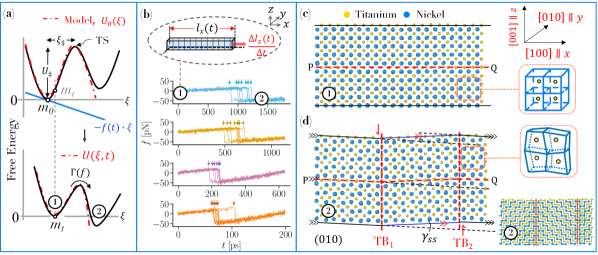
In the microscopic description, twinning is represented on a free energy profile, which can be imagined as a pair of local minima corresponding to the states, austenite–\scriptsize{1}⃝ and martensite–\scriptsize{2}⃝, separated by a barrier; Fig. 1(a), Top. Initially, under no force condition, the system is in an austenite state and is (meta)stable under thermal fluctuations. Austenitic states (unit-cells) evolve by stochastic crossing of the barrier, undergoing martensitic transitions aided by thermal activation. The crossing events, however, occur infrequently due to the large barrier size relative to thermal energy. This evolution is modelled by a probabilistic microscopic transport equation and provides a framework to understand the response relations of twinning force spectra and twinning force distribution. Gradually ramping the externally applied force, $f(t)\propto t$, from zero and linearly over time, $t$, under an isothermal condition, causes the initial system (in the austenite state) to shift away from equilibrium progressively. The free energy profile at equilibrium, $U_{0}(\xi)$, where $\xi$ denotes displacement, undergoes a downward tilt, contributing to a depression of the barrier; Fig. 1(a), Bottom. The instantaneous profile $U(\xi,t)$ is obtained by subtracting $\xi\cdot f(t)$ from $U_{0}(\xi)$. If a harmonic potential approximation of $U_{0}(\xi)$ is considered at $\xi_{0}$=0, with a vertical barrier of size $U_{0}(\xi=\xi_{\ddagger})-U_{0}(\xi=0)=U_{\ddagger}$ at $\xi=\xi_{\ddagger}$, then one finds for very small, imposed force, $f\ll(U_{\ddagger}/\xi_{\ddagger})$, a reduction of the original barrier from $U_{\ddagger}$ to $U_{\ddagger}(f)\approx U_{\ddagger}-f\xi_{\ddagger}$. Consequently, the flow of atomic configurations experiences lower resistance due to force-induced lowering of the barrier, which upregulates the austenite to martensite transformation rate, $\Gamma$, according to $\Gamma(f)\propto\exp[-U_{\ddagger}(f)/k_{B}T]\propto\exp(f\xi_{\ddagger}/k_{B}T)$. The exponential rate relation formally emerges if a model of free energy profile is incorporated into the statistical mechanics framework based on the Einstein-Smoluschowski evolution equation Risken (1989); Hanggi et al. (1990). It describes the spatiotemporal nature of the transition process through a relationship between the probability density of the instantaneous state population and the probability flux of states across the time-dependent free energy barrier. For large barriers, its solution provides the Kramers Kramers (1940) rate of escape yielding models for force-dependent rate of phase transition mediated twinning, $\Gamma(f|\dot{f})$, and twinning force distribution, $p(f_{\ddagger}|\dot{f})$, and its first moment, $\langle f_{\ddagger}\rangle({\dot{f}})$ at different levels of imposed force rates, $\dot{f}$, capturing rate-dependent properties of lattice twinning. Through these models and methods, such as maximum likelihood estimation, the statistical mechanical behaviour viewed through the lens of mechanical response spectra is examined and microscopic insights into twin evolution are derived. Specifically, estimates are drawn of the free energy profile, twin domain size, intrinsic kinetic constant, and activation barrier of solid-state structural phase transition. Knowledge of free energy landscape is crucial for the study of microstructural evolution in these systems using phase field models; for example, some of the current phase field models have used twin boundary energy and twin thickness Clayton and Knap (2016), ab initio calculations Liu et al. (2018), fractional strain energy Zhong and Zhu (2014), or latent heat Xi and Su (2021) to evaluate the parameters needed for the chemical part of free energy in such models. Thus, the free energy profile evaluated in this study can also serve as an accurate input to phase field models.

In the next section, we describe the methods— acquiring twinning response patterns using molecular dynamics simulations, processing twinning-associated observables, and applying a maximum likelihood estimation procedure for interpreting the resulting distributions. In the section on Results and Discussion, we review the microscopic theory, outlining the models of distribution and its first moment relevant to lattice twinning. Finally, we evaluate and discuss the outcomes of the statistical applications, providing insights into the free energy profile of the lattice twinning process.

 

 

Figure 1: Deformation twinning of titanium nickel single crystal. (a) (Top) Schematic of an equilibrium free energy profile (solid line) and a parameterized model, $U_{0}(\xi)$ (dot-dashed) used for reconstruction. The stationary state is denoted by $m_{0}\equiv\xi_{0}$=0. (Bottom) At a fixed temperatures, an imposed force, $f(t)$, causes the profile to incline by $-f(t).\xi$. (b) Schematic of molecular dynamics simulation box under constant uniaxial tensile deformation rate, ($\Delta l_{x}(t)/\Delta t$). Force-time traces, top to bottom, at ($\Delta l_{x}/\Delta t$) [Å/ps]: (i) 3.679 $\times$ 10^-4, (ii) 7.839 $\times$ 10^-4, (iii) 2.352 $\times$ 10^-3 and (iv) 7.525 $\times$ 10^-3. Short vertical arrows indicate twinning phase transition events. (c) Atomic configuration of \scriptsize{1}⃝—austenite phase, (010) projection. (d) Atomic configuration of twinned lattice \scriptsize{2}⃝. Miller indices refer to the orthogonal axes system of the parent lattice. Twin boundaries are denoted as TB₁ and TB₂, shear strain as $\gamma_{ss}$, and along PQ, a representative deformation is shown to highlight the change in atomic stacking in relation to (c). (Inset) Complexly patterned twinned martensite configuration, visualised as a display of bonds with lengths restricted to 3 Å  or less.

II Methods

II.1 Molecular Dynamics Simulations

Classical molecular dynamics Frenkel and Smit (2002); Ko et al. (2017); Srinivasan et al. (2018) calculations on titanium nickel (Ti:Ni=1:1) single crystals were performed using a modified embedded-atom method for the second-nearest neighbour interatomic potential Ko et al. (2015); Hale, L and Trautt, Z and Becker, C (2018). Along the $x$, $y$, and $z$ axes, the simulation box had lengths of 60 Å, 30 Å, and 30 Å, respectively, aligning with the [100], [010], and [001] directions of the periodic supercell, composed of 20 $\times$ 10 $\times$ 10 cubic unit cells. Periodic boundary conditions were chosen for all axes. Simulations were conducted and visualised, respectively using LAMMPS Plimpton (1995) and Ovito Stukowski (2010).

Nonequilibrium simulations were conducted to generate response force-time and force-displacement traces. During nonequilibrium simulations, the atomic system was evolved with a timestep of 1 fs within the NPT ensemble. The temperature was maintained at T=300 K, and pressures were constrained along the $y$ and $z$ axes at P=1.013 bar, employing the Nóse-Hoover approach Shinoda et al. (2004); Tuckerman et al. (2006). The damping times specified for temperature and pressure relaxation were, respectively, 0.7 ps and 1 ps. Thus, the system underwent relaxation within a few picoseconds, many orders of magnitude faster in kinetics than the structural transformation itself. The propagation of every tensile simulation had ensued from a random atomic configuration (microstate), which was sampled from the equilibrium (i.e., under no imposed force) isothermal-isobaric distribution of the system, prepared through 0.5-1 ns, to allow for its relaxation.

Homogeneous strain was applied to the simulation box, with the box dimension along $x$ axis, increasing in equal increments every timestep. The simulation trajectories and response traces were acquired at the following rates of uniaxial extension, ($\Delta l_{x}/\Delta t$), [Å/ps]: (i) 9.03 $\times$ 10^-5, (ii) 1.79 $\times$ 10^-4, (iii) 3.679 $\times$ 10^-4, (iv) 7.839 $\times$ 10^-4, (v) 2.352 $\times$ 10^-3, (vi) 7.525 $\times$ 10^-3 and (vii) 2.35 $\times$ 10^-2. The number of independent nonequilibrium simulations performed for tensile extensional rates (i)-(ii) was 30, and (iii)-(vii) was 400. The maximal strain was constrained within 2.5 % for elastic twin generation. At every timestep, the system’s net force that was generated by the imposed deformation was calculated using $f(t)=(A_{xx}/n)\sigma_{xx}(t)$. Here, $\sigma_{xx}$ represents the normal stress component of the internal stress tensor, defined through an expression of the system’s virial stress Thompson et al. (2009), and ($n/A_{xx}$) is the number density of atoms in the plane with a normal vector parallel to $x$ axis. The timescales of the applied strain rates were much smaller than the internal relaxation rate of the atomic system. With this criterion, on average, the externally imposed force, $f_{ext}$, remained in balance with the instantaneous force developed in the system, $\langle f(t)\rangle$, that is, $f_{ext}=\langle f(t)\rangle$.

II.2 Critical forces, normalised histograms, and force spectra

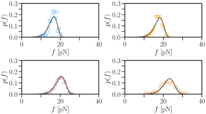
The steps for the retrieval of critical forces, histograms and force spectra from the molecular dynamics simulations are described. The force-time traces serve as the primary data and are processed to give the probability density functions (PDF) of critical forces for a given deformation rate. Representative samples of $f$-$t$ traces are displayed in Fig. 1(b). For the extraction of PDFs, the transition time, $t_{\ddagger}$, at which peak force occurs (before the transition) is identified, followed by its extraction from every $f$-$t$ trace, for all strain rates. Then, the transition time is converted to force value by multiplying with force-rate [$\dot{f}=\partial\langle f(t)\rangle/\partial t$], computed from the gradient of the averaged $f$-$t$ trace, denoted as $\langle f(t)\rangle$, in a small time interval near $t=0$. Corresponding to uniaxial tensile deformation rates ($\Delta l_{x}/\Delta t$) imposed, the following are the estimates of force rates $\dot{f}$, [pN/ps] observed: (i) 3.246 $\times$ 10^-3, (ii) 7.137 $\times$ 10^-3, (iii) 1.482 $\times$ 10^-2, (iv) 3.097 $\times$ 10^-2, (v) 9.452 $\times$ 10^-2, (vi) 2.927 $\times$ 10^-1, and (vii) 9.242 $\times$ 10^-1. Finally, the set of critical transition (or twinning) forces $\{f_{{\ddagger}}|\dot{f}\}$ for a given $\dot{f}$ is translated into a normalised histogram, $\widehat{p}(f|\dot{f})$, as shown in Fig. 2, and its first moment (mean), $\langle f\rangle(\dot{f})$, computed in dependence of the measured force rates; Fig. 3. The symbol $\wedge$ over a variable is used as a convention to distinguish that variable from its estimated value.

II.3 Estimation of parameterised landscape

Estimates of the landscape parameters—the free energy barrier, barrier location and intrinsic frequency of phase transition were obtained independently from statistical fits of the respective models of the PDF of critical twinning force, and the PDF’s first moment versus imposed forcing rates. In the first case, the PDF of critical force of lattice twinning, Eq. (6), was fit to the response observable $\widehat{p}(f;\dot{f})$ using the method of maximum likelihood estimation (MLE) Hastie et al. (2009), which is a statistical approach of parameter inference for models of distribution functions. It allows the determination of the model landscape that is most likely to have generated a random sample of phase transition forces $\{f_{ij}\}\equiv f_{11},f_{21},\cdots,f_{ij},\cdots$, which were retrieved from the force response data at different levels of strain rates or equivalent force rates, $\dot{f}$, as applicable in the present case. See section III.B for the form of the free energy profile. The critical force is denoted as $f_{ij}$ for the $i$-th sample trace, measured at a force rate $\dot{f_{j}}$. Here, $i=1,\ldots,S$, where $S$=400 is the sample size of the traces recorded for the $j$-th force rate, and $j=1,\ldots,N_{r}$ where $N_{r}$=4 is the number of distinct strain rates used for performing MLE. Denote the PDF of transition force vector $\{f_{ij}\}$ as $p(\{f_{ij}\}|\vec{w})$ for a given parameter vector $\vec{w}\equiv\{U_{\ddagger},x_{\ddagger},\Gamma_{0}\}$, which defines the free energy profile. Noting that each observation $f_{ij}$ is statistically independent, the PDF of $\{f_{ij}\}$ can be expressed as a product of the PDF of individual observations: $p(\{f_{ij}\}|\vec{w})=p(f_{11}|\vec{w})p(f_{12}|\vec{w})\ldots p(f_{SN_{r}}|\vec{w})$. According to MLE, a likelihood function $L_{mle}$ of the set of parameters $\vec{w}$, given a set $\{f_{ij}\}$, is defined as:

$$L_{mle}(\vec{w}|\{f_{ij}\})=\prod_{j=1}^{N_{r}}\prod_{i=1}^{S}p(f_{ij};\vec{w}).$$ (1)

An individual probability, $p(f_{ij};\vec{w})$, is given by the model Eq. (6), while the products are computed over the set of phase transition events observed, totalling $S_{j}\times N_{r}$ = 1600 events. Thus, the likelihood function evaluates how well a given landscape describes a transition force distribution. The log-likelihood, $(\ln L_{mle})$, function was maximised by varying $\vec{w}$, using the Nelder-Mead nonlinear optimising algorithm SciPy Community (2023); Nelder and Mead (1965), within a tolerance value on $(\ln L_{mle})$, set for achieving convergence of the algorithm, providing the most likely landscape parameters. In the second case, the model of first moment, Eq. (8), was fit to the expectation value of the distributions, $\langle\widehat{f}\rangle(\dot{f})$, using least square regression. Minimisation of the sum of squared residuals (that is, differences) between predicted and actual values was achieved using the conjugate gradient algorithm, giving optimal landscape parameters and standard errors (s.e); Table 1.

 

 

Figure 2: Probability density distributions of critical force of twinning. Shown are the PDFs, $p(f)$, of phase transition forces $f_{\ddagger}$ at deformation rates [Å/ps] (i) 3.679 $\times$ 10^-4 ($\square$), (ii) 7.839 $\times$ 10^-4 ($\mathord{\mathchoice{\leavevmode\resizebox{}{6.75pt}{\leavevmode\hbox{\raisebox{0.0pt}{$\displaystyle\bigcirc$}}}}{\leavevmode\resizebox{}{6.75pt}{\leavevmode\hbox{\raisebox{0.0pt}{$\textstyle\bigcirc$}}}}{\leavevmode\resizebox{}{4.72499pt}{\leavevmode\hbox{\raisebox{0.0pt}{$\scriptstyle\bigcirc$}}}}{\leavevmode\resizebox{}{3.375pt}{\leavevmode\hbox{\raisebox{0.0pt}{$\scriptscriptstyle\bigcirc$}}}}}$), (iii) 2.352 $\times$ 10^-3 ($\triangle$) and (iv) 7.525 $\times$ 10^-3 ($\Diamond$). Solid lines depict maximum likelihood estimated fits of Eq. (6) using a single set of optimum parameters given in Table 1.

III Results and Discussions

III.1 Transition force distribution is a defining characteristic of a twinning mechanism

Consistent with the behaviour expectation for an elastic solid, linear stress-strain and force-time traces were initially observed when subjecting single crystalline titanium nickel in the austenite (cubic) phase to a constant uniaxial tensile extension rate. This was followed by a sharp drop in stress or force on encountering a phase transition, leading to a change in symmetry of the lattice to a martensite phase and the creation of twin planes, which served to relieve the stress in the system. The twinned lattice displays stacking faults, which are defects in the stacking sequence of the atomic planes of the lattice. Representative atomic configurations, before and after the occurrence of phase transition, are depicted in Fig. 1(c) and (d), respectively. The twin boundaries TB₁ and TB₂ are shown as vertical dashed lines parallel to (100). In the twinned supercell, each lattice point had shifted along the direction [001] through a displacement in proportion to its perpendicular distance from the twin boundary. Representative faults in the stacking of (100) planes can be viewed along the line PQ on the plane of shear (010) in the transformed configuration Crocker and Bevis (1970); Christian (2002). The inherent stochasticity of the martensitic transformation is evident from the variations in the critical twinning forces observed over independent realisations of the system’s trajectory under identical conditions. The hallmarks of a transition mechanism are captured by the distribution of critical forces, represented in the conditional probability density, $\widehat{p}(f|\dot{f})$; refer to Fig. 2. To quantify the strain rate effects, we compute the statistical first moment $\langle f_{\ddagger}\rangle$ of twinning force distribution acquired at the different force rates $\dot{f}$. This twinning force spectra displays a nonlinear relation with considerable variation of strength; refer to Fig. 3. Interpreting the physical basis of twinning, as outlined in $p(f|\dot{f})$ and $\langle f_{\ddagger}\rangle(\dot{f})$, requires models of transition observables. Employing a microscopic theoretical approach, we illustrate how the response relations express fundamental characteristics of the solid-state transformation.

III.2 Quantitative description of phase transition linked force distribution

The transition observables are modelled using a formulation wherein twin formation occurs on a one-dimensional free energy landscape, $U_{0}(\xi)$; Fig. 1(a). The state of the crystal is denoted by $\xi$, an order parameter to track the change of state. In this perspective, atomic configurations pass from state \scriptsize{1}⃝ through a transition state (TS) to state \scriptsize{2}⃝. The TS acts as a barrier to the transition flux of the states since it has a higher free energy than both the parent and product configurations; see Fig. 1 (Top). The imposed time-dependent deformation, increasing monotonically in time, translates into increasing force levels and transition probabilities. The imposed force modifies the equilibrium profile, $U_{0}(\xi)$, such that $U(\xi,t)\approx U_{0}(\xi)-\langle f(t)\rangle\,\xi$. Here, $\langle f(t)\rangle$ denotes a statistical mean of the instantaneous force developed in the atomic system. It is computed as an average over the set of experiments or simulations performed at a constant rate of uniaxial tensile deformation:

$$\langle f(t)\rangle\approx\dot{f}t\equiv f(t).$$ (2)

The external perturbation causes the free energy landscape to slant. In addition, the curvature of the landscape and locations of free energy minima and the TS at $\xi=\xi_{\ddagger}$ are concurrently modified. These changes enable a faster turnover rate of the austenite to martensite, making the latter a preferred physical state.

For analytical modelling, consider a free energy function Garg (1995): $U_{0}(\xi)=U_{\ddagger}/2+(3U_{\ddagger}/2\xi_{\ddagger})(\xi-\xi_{\ddagger}/2)-(2U_{\ddagger}/(\xi_{\ddagger})^{3})(\xi-\xi_{\ddagger}/2)^{3}$, where $U_{\ddagger}$ is the free energy barrier (under no force condition), given as a difference in the free energy of TS and the free energy minimum of \scriptsize{1}⃝, and $\xi_{\ddagger}$ is the distance of the TS from the position ($m_{0}$) of free energy minimum of state \scriptsize{1}⃝. According to Einstein-Smoluschowski equation, the state probability density function, $P(\xi,t)$, is governed by $\partial_{t}P(\xi,t)=-\partial_{\xi}[-(k_{B}T/\eta)\,\partial_{\xi}P(\xi,t)+(-\partial_{\xi}U(\xi,t)/\eta)\,P(\xi,t)]$ Risken (1989); Hanggi et al. (1990), for the case of overdamped thermal activation. The equation assumes that the inertial term ($\ddot{\xi}$) is negligible based on strong drag forces captured via a frictional coupling, $\eta$, contributing to the dissipation of configurational fluctuations. An overview of the analytical solutions Risken (1989); Hanggi et al. (1990); Kramers (1940); Garg (1995); Dudko et al. (2003) are presented. The differential equation is simplified in terms of survival probability: $\Psi(t)=\int_{-\infty}^{\xi_{\ddagger}}P(\xi,t)d\xi$, defined as a cumulative distribution of the probability density of system state observed at time $t$ and domain, $-\infty<\xi<\xi_{\ddagger}$. $\Psi(t)$ gives the probability of austenite state to persist till time $t$. Assuming steady-state flux across the barrier, and the boundary at barrier position is absorbing, and further replacing variable $t$ with $f(t)$ via Eq. (2), the evolution equation can be recast into

$$-\partial_{f}\Psi(f)=\left[\Gamma(f)\Psi(f)\right]/\dot{f}.$$ (3)

$\Gamma(f)$ is the force-dependent rate of austenite to martensite transformation:

$$\Gamma(f)\approx\gamma(f)\;{\exp\left(\Delta U_{\ddagger}(f)/k_{B}T\right)},\\$$ (4)

the force-dependent terms of $\gamma(f)=\Gamma_{0}\left(1-(f/f_{c})\right)^{1/2}$ is the attempt frequency of atomic configurations to change state and $\Delta U_{\ddagger}(f)={U_{\ddagger}\left(1-\left\{1-(f/f_{c})\right\}^{3/2}\right)}$ is the change in barrier with force $f$. The maximal force to turnover austenitic state is $f_{c}\equiv(3U_{\ddagger}/2\xi_{\ddagger})$. The prefactor in the attempt frequency, at $f$=0, is given as $\Gamma_{0}=\{1/(2\pi\eta)\}\cdot(6U_{\ddagger}/{\xi_{\ddagger}}^{2})\;e^{-U_{\ddagger}/kT}$. The survival probability, $\psi(f)$, derived from Eq. (3) is

$$\psi(f)=\exp{\left\{\mu_{0}-\mu(f)\left(1-(f/f_{c})\right)^{-1/2}\right\}},$$ (5)

where $\mu(f)\equiv(\Gamma(f)\,k_{B}T)/(\dot{f}\,\xi_{\ddagger})$. As the imposed force increases, the survival probability of austenite decreases rapidly, from $\psi$($f$=0)=1, approaching zero as $f$ approaches $f_{c}$, since the austenite microstates progressively switch to martensite. The model PDF is obtained by substituting Eq. (5) in $p(f|\dot{f})=-\partial_{f}\psi$:

$$p(f\,|\,\accentset{\mbox{\large.}}{f})=\left\{\frac{\Gamma(f)}{\accentset{\mbox{\large.}}{f}}\right\}\exp{\left\{\mu_{0}-\mu(f)\left(1-(f/f_{c})\right)^{-1/2}\right\}}.$$ (6)

Here, $\mu_{0}\equiv\mu(f=0)$ is the rate $((k_{B}T)\cdot\Gamma_{0})$ of thermal energy transfer across the barrier at equilibrium, expressed as a fraction of the absorption rate of lattice strain energy, $(\xi_{\ddagger}\dot{f})$, due to the imposed forcing. The analytical model, Eq. (6), along with maximum likelihood estimation, enables the deduction of free energy profile, interaction range, and intrinsic kinetics governing the phase transition linked to the twinning mode of deformation.

III.3 Nonlinear relationship between twinning force and imposed loading rate

Figure 3: Mean force of lattice twinning vs force rate. First moment of $p(f|\dot{f})$, at different rates of tensile force rates $\dot{f}$ [pN/ps]. (Solid line) Least square regression model, Eq. (8). (Inset) Predicted free energy profile using best-fit parameters of Eq. (8) given in Table 1.

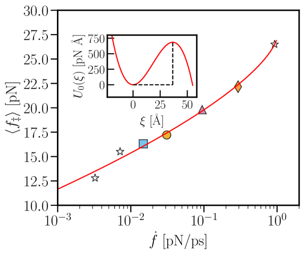
Fig. 3 (symbols) shows the relation between mean transition force to twin a lattice and the imposed force rate obtained from simulations. It shows a higher strength of the lattice (austenite) to twinning in the fast loading rate regime and lower strength at slower loading rates. In quantitative terms, a doubling of strength correlates with an approximately 300-fold increase in the force rate compared to the lowest imposed deformation rate in this study. It can be explained from the shift in energy minimum initially positioned on $m_{0}$ = 0 to the right, $m_{t}$, a configuration with a higher deformation associated landscape force, as the landscape leans downwards; Fig. 1(a) and (b). Consequently, under external perturbation, most configurations escape the free energy well beyond the value $\xi=m_{t}$ instead of the equilibrium value $\xi=m_{0}$. Since the landscape force $f_{L}(\xi=m_{t})$ is larger than $f_{L}(\xi=m_{0})$, this translates, on average, a higher force requirement for the escape of the atomic configurations still extant in the austenitic state.

The relation between the expectation value of the twinning transition force $\langle f_{\ddagger}\rangle$ vs. $\dot{f}$ can be derived as follows Friddle (2008). Integration of Eq. (3), $\dot{f}\int_{1}^{\psi}d\psi/\psi=-\int_{0}^{f}\Gamma(f)df$, after substituting Eq. (4) gives:

$$f(\omega)=f_{c}\left[1-\left\{1-\omega\right\}^{2/3}\right],$$ (7)

where $\omega(\psi)=(U_{\ddagger}/(k_{B}T))^{-1}\ln\left(1-\mu_{0}\ln\psi\right)$. Then, an expression for the expectation value (of the transition force) can be evaluated by a series expansion of $f(\omega)$ in the vicinity of $\omega=\langle\omega\rangle$ where $\langle\omega\rangle=\int_{0}^{1}\omega(\psi)d\psi$. This step is followed by performing an ensemble average of the series expansion: $\langle f\rangle=f(\langle\omega\rangle)+(1/2)\langle(\omega-\langle\omega\rangle)^{2}\rangle f^{\prime\prime}(\langle\omega\rangle)+\cdots\approx f(\langle\omega\rangle)$. The higher-order terms $f^{\prime\prime}(\langle w\rangle)$ and beyond are small and neglected. Finally, the required expression is obtained

$$\langle f\rangle\cong f_{c}\left[1-\left\{1-e^{\mu_{0}}E_{1}(\mu_{0})/(U_{\ddagger}/(k_{B}T))\right\}^{2/3}\right]\equiv\langle f_{\ddagger}\rangle\\$$ (8)

where $E_{1}(\mu_{0})=\int_{\mu_{0}}^{\infty}\frac{e^{-z}}{z}dz$ is an exponential integral Abramowitz and Stegun (1972). The physical basis of this twin law is thus a consequence of the time-dependent remodelling of the positions of austenite’s local minimum and transition state and the height of the barrier during the time course of deformation.

III.4 Response relations reflect fundamental properties of solid-state transformation-mediated twinning

The strain rate effects of twinning force distribution and its spectra collected from molecular dynamics simulations are characterised using the statistical mechanics-based models described in the previous subsections. The PDF Eq. (6) was optimised via the method of maximum likelihood estimation to fit the simulated twinning distributions. The model with optimum parameters is plotted for all strain rates in Fig. 2, solid lines. Whereas the line of regression for Eq. (8), which captures the simulated pattern, $\langle f\rangle(\dot{f})$, is plotted as a solid line in Fig. 3. The values of the optimal model parameters and standard errors (s.e) for both cases are given in Table 1. Both models effectively capture the variability observed in each simulated response type and across loading rates. The microscopic significance of the parameters is as follows. The estimate of $U_{\ddagger}$ suggests the stacking-fault free energy activation requirement for twin formation. Specifically, an average value of ($U_{\ddagger}/a^{2})$ involving 20 atomic layers of (100) planes gives $\approx$ 34 mJ/m² ($a\approx$ 3 Å  is lattice parameter), which lies in the range of estimates reported from density functional theory calculations Chowdhury and Sehitoglu (2017). In addition, $\xi_{\ddagger}$ and $\Gamma_{0}$, respectively, are estimates of the domain size of nanotwin produced and the intrinsic frequency of converting atomic configurations (unit cells) from the austenite to martensite phases. While the models demonstrate high explanatory performance, our focus has been on the material response under fast loading rates, or strain rates greater than 10^-4 Å/ps. Further scrutiny at lower force rates is required to establish their applicability for analyses of experimental responses. Nonetheless, the study addresses the nature of response-stimulus laws, utilising statistical mechanics to illustrate how such laws reflect the thermodynamic and kinetic features of the underlying phase change in the solid state.

Table 1: Estimates of free energy landscape parameters for lattice twinning in titanium nickel from statistical fits of Eqs. (6), and (8) to the respective deformation response data $\widehat{p}(f|\dot{f})$ and $\langle f\rangle(\dot{f})$ . Standard errors (s.e.) of parameters are specified in parenthesis.

Parameters	$p(f|\dot{f})$	$\langle f\rangle(\dot{f})$
$U_{{\ddagger}}$, pN Å	638.14	659
$\pm(\mathrm{s.e.})$	(9.62)	(38.6)
$\xi_{{\ddagger}}$, Å	29.2	36.1
$\pm(\mathrm{s.e.})$	(0.45)	(3.6)
$\Gamma_{0}$, 1/ps	3.96 $\times$ 10-7	6.12 $\times$ 10-8
$\pm(\mathrm{s.e.})$	(6.75 $\times$ 10-8)	(6 $\times$ 10-8)

IV Conclusion

Dynamic force spectroscopy allows probing the hidden variations in atomic scale interactions within crystal structures, offering insights into their mechanical stability. In the context of phase transition-mediated deformation twinning of titanium nickel, microscopic simulations indicate how systematic analyses of stochastic force responses at constant loading rates can reveal some previously unexplored stimulus-response laws of mechanical origin. The characteristic force spectrum—a relation between the first moment of critical force distribution to twin a lattice and the imposed rate of tensile deformation—arises from the microscopic twinning dynamics on a free energy landscape. The principles governing the force spectra are clarified through a statistical mechanical approach. Specifically, treating the twinning mechanism as a probabilistic process, in which the system state evolves in time from a physical state that is of austenite to a martensite over a one-dimensional free energy barrier, analytical models are described for reconciling the statistical patterns and force spectra under loading. This approach provides a robust explanation of the observables linked to the microscopic rate process of the martensitic transformation. In particular, statistical maximum-likelihood estimated fits of the analytical models to the twinning associated distributions enable the inference of the fundamental kinetic and thermodynamic information of the martensitic phase transformation. Quantifying energy barriers and activation mechanisms through free energy landscapes can offer key principles for designing shape-memory alloys with tailored properties. Further, these insights can be integrated into phase field models, accelerating materials development with desired microstructures. Within the scope of nanomechanics experiments, this work proposes probing force fluctuations to reveal the interplay between atomic interactions and mechanical behaviour of metallic systems.

Acknowledgement: The authors gratefully acknowledge the use of high performance computing facility and IT resources at BMU.

References

- Christian and Mahajan (1995) J. W. Christian and S. Mahajan, Prog. Mater. Sci. 39, 1 (1995).
- Beyerlein et al. (2014) I. J. Beyerlein, X. Zhang, and A. Misra, Annu. Rev. Mater. Res. 44, 329 (2014).
- Bhadeshia (2018) H. Bhadeshia, Geometry of Crystals, Polycrystals, and Phase Transformations (CRC Press, 2018).
- Uttam et al. (2020) P. Uttam, V. Kumar, K. H. Kim, and A. Deep, Mater. Des. 192, 108752 (2020).
- Otsuka and Wayman (1998) K. Otsuka and C. E. Wayman, Shape Memory Materials (Cambridge Univesity Press, 1998).
- Otsuka and Ren (2005) K. Otsuka and X. Ren, Prog. Mater. Sci. 50, 511 (2005).
- Bhattacharya et al. (2004) K. Bhattacharya, S. Conti, G. Zanzotto, and J. Zimmer, Nature 428, 55 (2004).
- Bhattacharya and James (2005) K. Bhattacharya and R. D. James, Science 307, 53 (2005).
- Jani et al. (2014) J. M. Jani, M. Leary, A. Subic, and M. A. Gibson, Mater. Des. 56, 1078 (2014).
- McCracken et al. (2020) J. M. McCracken, B. R. Donovan, and T. J. White, Adv. Mater. 32, 1 (2020).
- Pattamatta et al. (2014) S. Pattamatta, R. S. Elliott, and E. B. Tadmor, Proc. Natl. Acad. Sci. U. S. A. 111 (2014).
- Risken (1989) H. Risken, The Fokker‐Planck‐Equation. Methods of Solution and Applications (Springer-Verlag, Berlin, 1989).
- Seo et al. (2011) J. H. Seo, Y. Yoo, N. Y. Park, S. W. Yoon, H. Lee, S. Han, S. W. Lee, T. Y. Seong, S. C. Lee, K. B. Lee, et al., Nano Lett. 11, 3499 (2011).
- Dehm et al. (2018) G. Dehm, B. N. Jaya, R. Raghavan, and C. Kirchlechner, Acta Mater. 142, 248 (2018).
- Bhowmick et al. (2019) S. Bhowmick, H. Espinosa, K. Jungjohann, T. Pardoen, and O. Pierron, MRS Bull. 44, 487 (2019).
- Zhong et al. (2024) L. Zhong, Y. Zhang, X. Wang, T. Zhu, and S. X. Mao, Nat. Commun. 15, 1 (2024), ISSN 20411723.
- Maitra and Singh (2022) A. Maitra and B. Singh, Phys. Rev. Mater. 6, 043404 (2022).
- Ogata et al. (2005) S. Ogata, J. Li, and S. Yip, Phys. Rev. B - Condens. Matter Mater. Phys. 71, 1 (2005).
- Hatcher et al. (2009) N. Hatcher, O. Y. Kontsevoi, and A. J. Freeman, Phys. Rev. B 79, 020202 (2009).
- G Vishnu and Strachan (2010) K. G Vishnu and A. Strachan, Acta Mater. (2010), ISSN 13596454.
- Zarkevich and Johnson (2014) N. A. Zarkevich and D. D. Johnson, Phys. Rev. Lett. 113, 10797114 (2014).
- Chowdhury and Sehitoglu (2017) P. Chowdhury and H. Sehitoglu, Prog. Mater. Sci. 88, 49 (2017).
- Niitsu et al. (2020) K. Niitsu, H. Date, and R. Kainuma, Scr. Mater. 186, 263 (2020).
- Kumar and Waghmare (2020) P. Kumar and U. V. Waghmare, Materialia 9, 100602 (2020).
- Tang et al. (2018) X. Z. Tang, Q. Zu, and Y. F. Guo, J. Appl. Phys. 123 (2018).
- Yan and Sharma (2016) X. Yan and P. Sharma, Nano Lett. 16, 3487 (2016).
- Müller and Seelecke (2001) I. Müller and S. Seelecke, Math. Comput. Model. 34, 1307 (2001).
- Falk (1980) F. Falk, Acta Metall. 28, 1773 (1980).
- Falk (1983) F. Falk, Z. Phys. B 51, 177 (1983).
- Hanggi et al. (1990) P. Hanggi, P. Talkner, and M. Borkovec, Rev. Mod. Phys. 62, 251 (1990).
- Kramers (1940) H. Kramers, Physica 7, 284 (1940).
- Clayton and Knap (2016) J. D. Clayton and J. Knap, Comput. Methods Appl. Mech. Eng. 312, 447 (2016).
- Liu et al. (2018) C. Liu, P. Shanthraj, M. Diehl, F. Roters, S. Dong, J. Dong, W. Ding, and D. Raabe, Int. J. Plast. 106, 203 (2018).
- Zhong and Zhu (2014) Y. Zhong and T. Zhu, Acta Mater. 75, 337 (2014).
- Xi and Su (2021) S. Xi and Y. Su, Materials (Basel). 14, 1 (2021).
- Frenkel and Smit (2002) D. Frenkel and B. Smit, Understanding Molecular Simulation: From Algorithms to Applications, vol. 1 of Computational Science Series (Academic Press, San Diego, 2002), 2nd ed.
- Ko et al. (2017) W.-S. Ko, S. B. Maisel, B. Grabowski, J. B. Jeon, and J. Neugebauer, Acta Materialia 123, 90 (2017).
- Srinivasan et al. (2018) P. Srinivasan, L. Nicola, and A. Simone, Comput. Mater. Sci. 154, 25 (2018).
- Ko et al. (2015) W. S. Ko, B. Grabowski, and J. Neugebauer, Phys. Rev. B. 92, 134107 (2015).
- Hale, L and Trautt, Z and Becker, C (2018) Hale, L and Trautt, Z and Becker, C, Interatomic potentials repository (2018), https://www.ctcms.nist.gov/potentials/, Last accessed on 01 Feb 2024.
- Plimpton (1995) S. Plimpton, J. Comput. Phys. 117, 1 (1995).
- Stukowski (2010) A. Stukowski, Modelling and Simulation in Materials Science and Engineering 18 (2010).
- Shinoda et al. (2004) W. Shinoda, M. Shiga, and M. Mikami, Phys. Rev. B - Condens. Matter Mater. Phys. 69, 16 (2004).
- Tuckerman et al. (2006) M. E. Tuckerman, J. Alejandre, R. López-Rendón, A. L. Jochim, and G. J. Martyna, J. Phys. A. Math. Gen. 39, 5629 (2006).
- Thompson et al. (2009) A. P. Thompson, S. J. Plimpton, and W. Mattson, The Journal of Chemical Physics 131, 154107 (2009).
- Hastie et al. (2009) T. Hastie, R. Tibshirani, and J. Friedman, The Elements of Statistical Learning: Data Mining, Inference, and Prediction (Springer, 2009).
- SciPy Community (2023) SciPy Community, Scipy documentation (2023), https://docs.scipy.org/doc/scipy/reference/optimize.html, Last accessed on 01 Feb 2024.
- Nelder and Mead (1965) J. A. Nelder and R. Mead, The Computer Journal 7, 308 (1965).
- Crocker and Bevis (1970) A. G. Crocker and M. Bevis, in The Science, Technology and Application of Titanium, edited by R. Jaffee and N. Promisel (Pergamon Press, Oxford, 1970), p. 453.
- Christian (2002) J. W. Christian, in The Theory of Transformations in Metals and Alloys, edited by J. W. Christian (Pergamon, Oxford, 2002), pp. 23–78.
- Garg (1995) A. Garg, Phys. Rev. B 51, 15592 (1995).
- Dudko et al. (2003) O. K. Dudko, a. E. Filippov, J. Klafter, and M. Urbakh, Proc. Natl. Acad. Sci. U. S. A. 100, 11378 (2003).
- Friddle (2008) R. Friddle, Phys. Rev. Lett. 100, 138302 (2008).
- Abramowitz and Stegun (1972) M. Abramowitz and I. Stegun, Handbook of Mathematical functions (Dover, New York, 1972).