De la Vallée Poussin filtered polynomial approximation on the half line

Abstract

On the half line we introduce a new sequence of near–best uniform approximation polynomials, easily computable by the values of the approximated function at a truncated number of Laguerre zeros. Such approximation polynomials come from a discretization of filtered Fourier–Laguerre partial sums, which are filtered by using a de la Vallée Poussin (VP) filter. They have the peculiarity of depending on two parameters: a truncation parameter that determines how many of the $n$ Laguerre zeros are considered, and a localization parameter, which determines the range of action of the VP filter that we are going to apply. As $n\to\infty$, under simple assumptions on such parameters and on the Laguerre exponents of the involved weights, we prove that the new VP filtered approximation polynomials have uniformly bounded Lebesgue constants and uniformly convergence at a near–best approximation rate, for any locally continuous function on the semiaxis.
The theoretical results have been validated by the numerical experiments. In particular, they show a better performance of the proposed VP filtered approximation versus the truncated Lagrange interpolation at the same nodes, especially for functions a.e. very smooth with isolated singularities. In such cases we see a more localized approximation as well as a good reduction of the Gibbs phenomenon.

1 Introduction

The paper deals with the approximation of locally continuous functions $f$ defined on the positive half-line. The function $f$ we consider can exponentially grow at infinity or/and have an algebraic singularity at the origin. Measuring the approximation error with a suitable weighted uniform norm, the Weierstrass approximation theorem may be applied and $f$ can be approximated by polynomials at the desired precision.

The topic has been extensively studied by many authors, which were looking for a polynomial approximating sequence having optimal Lebesgue constants in spaces of locally continuous functions equipped with uniform weighted norms [9, 15, 3, 6, 8, 10].Based on Laguerre zeros, we mention the classical Lagrange interpolating polynomial for which in [9] it has been proved that the associated weighted Lebesgue constants diverge as $n^{\frac{1}{6}}$. In the same paper a ”remedium” was proposed to this bad behavior, by introducing a suitable additional node. In this case, sufficient and necessary conditions have been stated to get optimal Lebesgue constants growing with minimal order $\log n$. A truncated version of the latter Lagrange polynomial has been introduced and studied in [3, 6] by involving only a very reduced number of function evaluations. Also in this case we get optimal Lebesgue constants, under suitable sufficient conditions.

In the present paper we introduce new approximation polynomials based on the same data of the truncated Lagrange-Laguerre interpolation but able to provide uniformly bounded Lebesgue constants and a near-best convergence order for any locally continuous function on the semiaxis. Such polynomials are defined by discretizing some VP means, namely delayed arithmetic means of the Fourier-Laguerre partial sums.

We recall that in literature such continuous VP means have been introduced as an useful tool to prove several theoretical results [13, 14].

In the Jacobi case it is known that by discretizing VP means we get near-est approximation operators that preserve the polynomials up to certain degree, have uniformly bounded Lebesgue constants [18] and, in some cases, are interpolating too. Here we show that, in the Laguerre case, the interpolation property as well as the polynomial preservation are not ensured. But, all the same, we prove the uniform convergence at a near-best approximation rate with uniformly bounded Lebesgue constants, under suitable assumptions.

The outline of the paper is the following. In Section 2 the necessary notations and preliminary results are introduced. Section 3 concerns the definition and the properties of the new VP discrete approximation polynomials. Section 4 deals with the numerical experiments and, finally, Section 5 regards the conclusions.

2 Notations and preliminary results

Along all the paper the notation ${\mathcal{C}}$ will be used several times to denote a positive constant having different values in different formulas. We will write ${\mathcal{C}}\neq\mathcal{C}(a,b,\ldots)$ in order to say that $\mathcal{C}$ is independent of the parameters $a,b,\ldots$, and $\mathcal{C}=\mathcal{C}(a,b,\ldots)$ to say that $\mathcal{C}$ depends on $a,b,\ldots$. Moreover, if $A,B>0$ are quantities depending on some parameters, we will write $A\sim B,$ if there exists an absolute constant ${\mathcal{C}}>0$, independent on such parameters, such that ${\mathcal{C}}^{-1}B\leq A\leq{\mathcal{C}}B$.

For all $\gamma\geq 0,$ we will consider the weight $u(x)=x^{\gamma}e^{-x/2},$ and the space $C_{u}$ of all locally continuous functions on the half line (i.e., continuous in $]0,\infty[$) such that

$$\lim_{x\to\infty}(fu)(x)=0,\qquad\mbox{and, in the case $\gamma>0$, also}\qquad\lim_{x\to 0}(fu)(x)=0.$$

We will take the space $C_{u}$ equipped with the norm

$$\|f\|_{C_{u}}=\|fu\|:=\sup_{x\geq 0}\left|(fu)(x)\right|,$$

and for any compact set $D\subset[0,+\infty)$, we will use $\|f\|_{D}=\sup_{x\in D}|f(x)|$.

Note that functions in $C_{u}$ may grow exponentially as $x\to+\infty$, and may have an algebraic singularity at the origin.

Denoting by ${\mathbb{P}}_{n}$ the space of the algebraic polynomials of degree at most $n\geq 0$, we will consider the error of best approximation of $f\in C_{u}$ in ${\mathbb{P}}_{n}$

$$E_{n}(f)_{u}:=\inf_{P_{n}\in{\mathbb{P}}_{n}}\|(f-P_{n}){u}\|,$$ (1)

It is known that [4, 5, 11, 12]

$$\lim_{n\to\infty}E_{n}(f)_{{u}}=0,\qquad\forall f\in C_{u}.$$

For  smoother functions, we consider the Sobolev-type spaces of order $r\in{\mathbb{N}}$

$$W_{r}(u)=\left\{f\in C_{u}\ :\ f^{(r-1)}\in AC((0,+\infty))\mbox{ and }\ \|f^{(r)}\varphi^{r}u\|<+\infty\right\},$$

where $AC((0,+\infty))$ denotes the set of all functions which are absolutely continuous on every closed subset of $(0,+\infty)$ and $\varphi(x)=\sqrt{x}.$

We equip these spaces with the norm

$$\|f\|_{W_{r}(u)}:=\|fu\|+\|f^{(r)}\varphi^{r}u\|.$$

For any function $f\in W_{r}(u)$ the following estimate holds [1, 4]

$$E_{n}(f)_{{u}}\leq{\mathcal{C}}\frac{\|f\|_{W_{r}(u)}}{\sqrt{n^{r}}},\quad{\mathcal{C}}\neq{\mathcal{C}}(n,f).$$ (2)

2.1 Truncated Lagrange interpolation at the zeros of Laguerre polynomials

Let $w_{\alpha}(x)=e^{-x}x^{\alpha}$ be the Laguerre weight of parameter $\alpha>-1$ and let $\{p_{n}(w_{\alpha})\}_{n}$ be the corresponding sequence of orthonormal Laguerre polynomials with positive leading coefficients. Denoting by $x_{k}:=x_{n,k},\ k=1,\dots,n,$ the zeros of $p_{n}(w_{\alpha})$ in increasing order, we recall that (see [17])

$$\frac{{\mathcal{C}}}{n}<x_{1}<x_{2}<\ldots<x_{n}<4n+2\alpha-{\mathcal{C}}n^{\frac{1}{3}},\qquad{\mathcal{C}}\neq{\mathcal{C}}(n).$$ (3)

In the sequel, we will be interested in taking only a part of these zeros. More precisely, throughout the paper, the integer $j:=j(n)$ will denote the index of the last zero of $p_{n}(w_{\alpha})$ we consider. It is defined by

$$j=\min_{k=1,2,..,n}\left\{k:x_{k}\geq 4n\rho\right\},$$ (4)

with $0<\rho<1$ arbitrarily fixed,

We recall that, inside the segment $[0,x_{j}]$, the distance between two consecutive zeros of $p_{n}(w_{\alpha})$ can be estimated as follows

$$\Delta x_{k}\sim\Delta x_{k-1}\sim\sqrt{\frac{x_{k}}{n}},\qquad\quad\Delta x_{k}=x_{k+1}-x_{k},\qquad k=1,2,\dots,j.$$

With $j$ defined in (4), let $L_{n+1}^{*}(w_{\alpha},f)$ be the truncated Lagrange polynomial [6] defined by

$$L_{n+1}^{*}(w_{\alpha},f,x):=\sum_{k=1}^{j}f(x_{k})\ell_{n,k}(x),$$ (5)

where

$$\ell_{n,k}(x)=\frac{p_{n}(w_{\alpha},x)}{p^{\prime}_{n}(x_{k})(x-x_{k})}\frac{4n-x}{4n-x_{k}},\qquad k=1,2,\dots,j,$$ (6)

are the fundamental Lagrange polynomials corresponding to the zeros of $p_{n}(w_{\alpha},x)(4n-x)$.

It is known that the norm of the operator $L_{n+1}^{*}(w_{\alpha}):f\in C_{u}\to L_{n+1}^{*}(w_{\alpha},f)\in C_{u}$, i.e. the weighted Lebesgue constant

$$\|L_{n+1}^{*}(w_{\alpha})\|_{C_{u}}=\sup_{\|fu\|=1}\|L_{n+1}^{*}(w_{\alpha},f)u\|=\sup_{x\geq 0}\sum_{k=1}^{j}|\ell_{n,k}(x)|\frac{u(x)}{u(x_{k})},$$ (7)

diverges at least as $\log n$ when $n\to\infty$. To be more precise, the following result holds [6]

Theorem 2.1

[6] Let $w_{\alpha}(x)=e^{-x}x^{\alpha},\ \alpha>-1$ and $u(x)=e^{-\frac{x}{2}}x^{\gamma},\ \gamma\geq 0.$ Under the assumption

$$\max\left(0,\frac{\alpha}{2}+\frac{1}{4}\right)\leq\gamma\leq\frac{\alpha}{2}+\frac{5}{4},$$ (8)

we have

$$\|L_{n+1}^{*}(w_{\alpha},f)u\|\leq{\mathcal{C}}\|fu\|\log n,\quad\forall f\in C_{u},\qquad{\mathcal{C}}\neq{\mathcal{C}}(n,f).$$ (9)

Moreover, as regards the approximation of $f\in C_{u}$ provided by the polynomial $L_{n+1}^{*}(w_{\alpha},f)$ we recall the following

Theorem 2.2

[6, Th.2.2] For any $f\in C_{u},$ under the assumption (8), we have

$$\|(f-L_{n+1}^{*}(w_{\alpha},f))u\|\leq{\mathcal{C}}(\log n)\left[E_{N}(f)_{u}+e^{-An}\|fu\|\right],$$

where $N=\left\lfloor\left(\frac{\rho}{1+\rho}\right)n\right\rfloor\sim n$, and $A$ and ${\mathcal{C}}$ are positive constants independent of $n$ and $f$.

2.2 Ordinary and truncated Gauss-Laguerre rules

According to the previous notation, the Gauss-Laguerre rule on the nodes in (3) is given by

$$\int_{0}^{+\infty}f(x)w_{\alpha}(x)dx=\sum_{k=1}^{n}f(x_{k})\lambda_{n,k}(w_{\alpha})+R_{n}(f),\qquad n\in{\mathbb{N}},$$ (10)

where $\lambda_{n,k}(w_{\alpha})=\left[\sum_{j=0}^{n}p_{j}(x_{k})\right]^{-1}$ are the Christoffel numbers w.r.t. $w_{\alpha},$ and the remainder term satisfies

$$R_{n}(f)=0,\qquad\forall f\in{\mathbb{P}}_{2n-1}.$$ (11)

For any $f\in C_{u}$, under the assumption $\alpha-\gamma>-1$, the following estimate holds

$$|R_{n}(f)|\leq\ {\mathcal{C}}E_{2n-1}(f)_{u},\qquad{\mathcal{C}}\neq{\mathcal{C}}(n,f).$$

In [7] the “truncated” Gauss-Laguerre rule was introduced by using only the first $j$ zeros of $p_{n}(w_{\alpha})$, with $j$ defined in (4), i.e.

$$\int_{0}^{+\infty}f(x)w_{\alpha}(x)dx=\sum_{k=1}^{j}f(x_{k})\lambda_{n,k}(w_{\alpha})+R_{n,j}(f),$$ (12)

where

$$R_{n,j}(f)=0,\qquad\forall f\in\mathcal{P}_{n-1}^{*}:=\left\{p\in{\mathbb{P}}_{n-1}:p(x_{k})=0,\quad k>j\right\}.$$ (13)

In [6] the following estimate was proved under the assumption $\alpha-\gamma>-1$

$$|R_{n,j}(f)|\leq{\mathcal{C}}\ \left(E_{N}(f)_{u}+e^{-\mathcal{B}n}\|fu\|\right),\qquad\forall f\in C_{u},$$

where $N=\left\lfloor\left(\frac{\rho}{1+\rho}\right)n\right\rfloor\sim n$, and $\mathcal{B},{\mathcal{C}}>0$ are constants independent of $n,f$.

2.3 Cesaro and de la Vallée Poussin means

For any given $n\in{\mathbb{N}}_{0}=\{0,1,2,...\}$, let $S_{n}(w_{\alpha},f)\in{\mathbb{P}}_{n}$ the $n-$th Fourier sum of $f$ in the orthonormal system $\{p_{i}(w_{\alpha})\}_{i=0,1,..}$, namely

$$S_{n}(w_{\alpha},f,x)=\sum_{i=0}^{n}c_{i}(f)p_{i}(w_{\alpha},x)$$

with Fourier coefficients defined as

$$c_{i}(f)=\int_{0}^{+\infty}f(t)p_{i}(w_{\alpha},t)w_{\alpha}(t)dt.$$ (14)

For all $n\in{\mathbb{N}}=\{1,2,....\}$, we recall the Cesaro means are defined as arithmetic means of the first $n-1$ Fourier sums, i.e.

$$\sigma_{n}(w_{\alpha},f,x)=\frac{1}{n}\sum_{k=0}^{n-1}S_{k}(w_{\alpha},f,x)=\sum_{i=0}^{n-1}\mu_{n,i}^{m}c_{i}(f)p_{i}(w_{\alpha},x),$$ (15)

In [16] simple necessary and sufficient conditions have been stated in order that the map $\sigma_{n}(w_{\alpha}):C_{u}\to C_{u}$ is uniformly bounded w.r.t. $n\in{\mathbb{N}}$.

Theorem 2.3

[16, Theorems 1 and 5]
For all $\alpha>-1$, let $w_{\alpha}(x)=e^{-x}x^{\alpha}$ and $u(x)=x^{\beta}\sqrt{w_{\alpha}(x)}$. The map $\sigma_{n}(w_{\alpha}):C_{u}\to C_{u}$ is uniformly bounded w.r.t. $n\in{\mathbb{N}}$, i.e. we have

$$\|\sigma_{n}(w_{\alpha},f)u\|\leq{\mathcal{C}}\|fu\|,\quad\forall f\in C_{u},\quad\forall n\in{\mathbb{N}},\qquad{\mathcal{C}}\neq{\mathcal{C}}(n,f),$$ (16)

if and only if the following bounds are satisfied

$$-\min\left\{\frac{\alpha}{2},\frac{1}{4}\right\}<\beta<1+\min\left\{\frac{\alpha}{2},\frac{1}{4}\right\},\qquad\mbox{and}\qquad-\frac{1}{2}\leq\beta\leq\frac{7}{6}$$ (17)

Now, besides $n\in{\mathbb{N}}$, let us take an additional parameter $m\in{\mathbb{N}}$ such that $0<m<n$, and, for a given function $f$, let us consider the VP means, namely the following delayed arithmetic means of Fourier sums

$$\mathcal{V}_{n}^{m}(w_{\alpha},f,x)=\frac{1}{2m}\sum_{k=n-m}^{n+m-1}S_{k}(w_{\alpha},f,x),$$ (18)

From a computational point of view, this is equivalent to

$$\mathcal{V}_{n}^{m}(w_{\alpha},f,x)=\sum_{i=0}^{n+m-1}\mu_{n,i}^{m}c_{i}(f)p_{i}(w_{\alpha},x),$$ (19)

that is a filtered version of $S_{n+m-1}(w_{\alpha},f)$ with filter coefficients $\mu_{n,i}^{m}$ defined as

$$\mu_{n,i}^{m}:=\left\{\begin{array}[]{cl}1&\mbox{if}\quad i=0,\ldots,n-m,\\[7.22743pt] \displaystyle\frac{n+m-i}{2m}&\mbox{if}\quad n-m+1\leq i\leq n+m-1.\\ \end{array}\right.$$ (20)

The filtered VP polynomial $\mathcal{V}_{n}^{m}(w_{\alpha},f)\in{\mathbb{P}}_{n+m-1}$ can be also rewritten in integral form as

$$\mathcal{V}_{n}^{m}(w_{\alpha},f,x)=\int_{0}^{+\infty}f(t)v_{n}^{m}(x,t)w_{\alpha}(t)dt,$$ (21)

where

$$v_{n}^{m}(x,t)=\frac{1}{2m}\sum_{r=n-m}^{n+m-1}K_{r}(x,t),\qquad\mbox{and}\qquad K_{r}(x,t)=\sum_{i=0}^{r}p_{i}(w_{\alpha},x)p_{i}(w_{\alpha},t)$$

are the VP and Darboux kernels, respectively.

Note that $v_{n}^{m}(x,t)=v_{n}^{m}(t,x)$ is a polynomial of degree $n+m-1$ in both the variables that can be represented as

$$v_{n}^{m}(x,t)=\sum_{i=0}^{n+m-1}\mu_{n,i}^{m}p_{i}(w_{\alpha},x)p_{i}(w_{\alpha},t).$$

An advantage of taking VP means instead of Cesaro means is given by the following invariance property

$$\mathcal{V}_{n}^{m}(w_{\alpha},P)=P,\quad\forall P\in{\mathbb{P}}_{n-m}.$$ (22)

Such preservation property allows us to investigate the approximation provided by $\mathcal{V}_{n}^{m}(w_{\alpha},f)$ in $C_{u}$, by estimating the norm of the operator map $\mathcal{V}_{n}^{m}(w_{\alpha}):C_{u}\to C_{u}$, that is

$$\|\mathcal{V}_{n}^{m}(w_{\alpha})\|_{C_{u}}=\sup_{\|fu\|=1}\|\mathcal{V}_{n}^{m}(w_{\alpha},f)u\|=\sup_{x\geq 0}\left[u(x)\int_{0}^{+\infty}|v_{n}^{m}(x,t)|\frac{w_{\alpha}(t)}{u(t)}dt\right].$$ (23)

To this aim, we introduce the following notation concerning the degree parameters $m,n\in{\mathbb{N}}$ defining the VP mean:

$$m\sim n m<n\leq{\mathcal{C}}m,\qquad\qquad\mbox{holds with ${\mathcal{C}}>1$ independent of $n,m$},$$ iff (24)

$$m\approx n m<c_{1}m\leq n\leq c_{2}m,\quad\mbox{holds with $c_{2}\geq c_{1}>1$ independent of $m,n$.}$$ iff (25)

Note that $m\sim n$ agrees with the notation introduced in Section 2 while $m\approx n$ is a stronger condition that ensures $(n-m)\sim n$ holds too.

If we take the additional parameter $m$ such that $m\sim n$ then from Theorem 2.3 we easily deduce the uniform boundedness of VP operator $\mathcal{V}_{n}^{m}(w_{\alpha})$ in $C_{u}$ for suitable choices of the weights $w_{\alpha}$ and $u$. More precisely, we have the following

Theorem 2.4

Let the weight function $w_{\alpha}(x)=e^{-x}x^{\alpha}$ and $u(x)=e^{-\frac{x}{2}}x^{\gamma},$ satisfy the following bounds

$$\max\left\{\frac{\alpha}{2}-\frac{1}{4},\ 0\right\}<\gamma<\min\left\{\frac{\alpha}{2}+\frac{7}{6},\ \alpha+1\right\}$$ (26)

then, for any couple of positive integers $m\sim n$, the map $\mathcal{V}_{n}^{m}(w_{\alpha}):C_{u}\to C_{u}$ is uniformly bounded w.r.t. $n$ and $m$, i.e.

$$\|\mathcal{V}_{n}^{m}(w_{\alpha},f)u\|\leq{\mathcal{C}}\|fu\|,\quad\forall f\in C_{u},\quad\forall m\sim n,\qquad{\mathcal{C}}\neq{\mathcal{C}}(n,m,f).$$ (27)

Proof of Theorem 2.4 Taking into account that

$$\mathcal{V}_{n}^{m}(w_{\alpha},f)=\frac{n+m}{2m}\sigma_{n+m}(w_{\alpha},f)-\frac{n-m}{2m}\sigma_{n-m}(w_{\alpha},f),$$

the statement follows by using the assumption (24) that implies

$$\frac{n+m}{2m}\leq\frac{{\mathcal{C}}+1}{2},\qquad\mbox{and}\qquad\frac{n-m}{2m}\leq\frac{{\mathcal{C}}-1}{2},\qquad{\mathcal{C}}\neq{\mathcal{C}}(n,m),$$

and applying Theorem 2.3 with $\beta=\gamma-\frac{\alpha}{2}$, that satisfies (17) by virtue of (26). $\diamondsuit$

Hence, concerning the error estimate the following result can be deduced

Theorem 2.5

Let the weight function $w_{\alpha}(x)=e^{-x}x^{\alpha}$ and $u(x)=e^{-\frac{x}{2}}x^{\gamma},$ satisfy (26). Then, for any $f\in C_{u}$ and for all $m\sim n$, we have

$$E_{n+m-1}(f)_{u}\leq\|[f-\mathcal{V}_{n}^{m}(w_{\alpha},f)]u\|\leq{\mathcal{C}}E_{n-m}(f)_{u},\qquad{\mathcal{C}}\neq{\mathcal{C}}(n,m,f),$$ (28)

Moreover, if $m\approx n$ then we get

$$\|f-\mathcal{V}_{n}^{m}(w_{\alpha},f)\|_{C_{u}}\sim E_{n}(f)_{u},\qquad\forall f\in C_{u}$$ (29)

with the constants in $\sim$ independent of $n,m,f$

Proof of Theorem 2.5

The first inequality in (28) trivially follows from $\mathcal{V}_{n}^{m}(w_{\alpha},f)\in{\mathbb{P}}_{n+m-1}$.

The second inequality in (28) can be deduced by means of (22) and (27) that yield

$$\|[f-\mathcal{V}_{n}^{m}(w_{\alpha},f)]u\|\leq\|(f-P)u\|+\|\mathcal{V}_{n}^{m}(w_{\alpha},\ f-P)u\|\leq{\mathcal{C}}\|(f-P)u\|,\qquad\forall P\in{\mathbb{P}}_{n-m}$$

and the statement follows by taking, at both the sides, the infimum w.r.t. $P\in{\mathbb{P}}_{n-m}$. $\diamondsuit$

3 VP filtered discrete approximation

In the previous section, we have seen that for any $f\in C_{u}$ and suitable choices of $w_{\alpha}$, the polynomials $\{\mathcal{V}_{n}^{m}(w_{\alpha},f)\}_{m\approx n}$ provide a near–best approximation of $f$. However, their construction requires the knowledge of the Fourier coefficients of the function $f$. To overcome this problem, in this section we introduce the polynomial ${V}_{n}^{m}(w_{\alpha},f)$, that we define as a discrete version of $\mathcal{V}_{n}^{m}(w_{\alpha},f)$. To be more precise, with $j=j(n)$ defined in (4), we apply the Gauss-Laguerre rule in (12) to the coefficients $c_{i}(f)$ in (14), getting

$$c_{n,i}^{(j)}(f)=\sum_{k=1}^{j}f(x_{k})p_{i}(w_{\alpha},x_{k})\lambda_{n,k}(w_{\alpha})$$ (30)

Hence, similarly to (19) we define the following discrete VP filtered approximation polynomials

$${V}_{n}^{m}(w_{\alpha},f,x)=\sum_{i=0}^{n+m-1}\mu_{n,i}^{m}c_{n,i}^{(j)}(f)p_{i}(w_{\alpha},x),\qquad 0<m<n$$ (31)

that can be equivalently written as

$${V}_{n}^{m}(w_{\alpha},f,x)=\sum_{k=1}^{j}f(x_{k})\Phi_{n,k}^{m}(x),\qquad x\geq 0$$ (32)

with $j=j(n)$ defined in (4), and

$$\Phi_{n,k}^{m}(x)=\lambda_{n,k}(w_{\alpha})v_{n}^{m}(x,x_{k})=\lambda_{n,k}(w_{\alpha})\sum_{i=0}^{n+m-1}\mu_{n,i}^{m}p_{i}(w_{\alpha},x_{k})p_{i}(w_{\alpha},x).$$ (33)

In Fig. 1 we show, as an example, the graphics of the fundamental polynomial $\Phi_{n,k}^{m}(x)$, for $n$ and $k$ fixed, and $m$ varying. As we can see for increasing $m$ the oscillations of $\Phi_{n,k}^{m}(x)$ progressively dampen. The major oscillating behavior is presented by the fundamental Lagrange polynomial $\ell_{n,k}(x)$ that are plotted in the same figure.

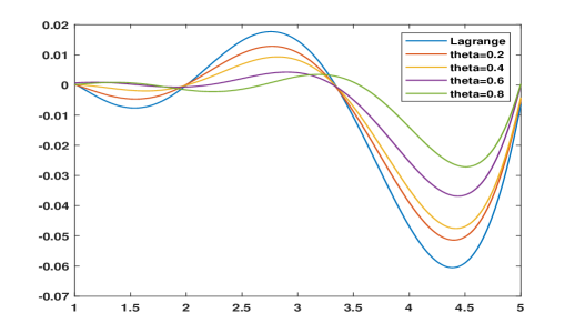
Figure 1: Plots of the fundamental polynomials $\ell_{n,k}(x)$ and $\Phi_{n,k}^{m}(x)$ for $\alpha=-0.5$, $n=15$, $k=7$, and $m=\lfloor\theta n\rfloor$

We remark that, similarly to $\mathcal{V}_{n}^{m}(w_{\alpha},f)$, for any function $f$ we have ${V}_{n}^{m}(w_{\alpha},f)\in{\mathbb{P}}_{n+m-1}$, but in the case $f=P\in{\mathbb{P}}_{n-m}$ the invariance property (22) does not apply to $V_{n}^{m}(w_{\alpha},f)$.

It can be easily proved that the norm of the operator map ${V}_{n}^{m}(w_{\alpha}):C_{u}\to C_{u}$ takes the following form

$$\|{V}_{n}^{m}(w_{\alpha})\|_{C_{u}}=\sup_{\|fu\|=1}\|{V}_{n}^{m}(w_{\alpha},f)\|=\sup_{x\geq 0}\sum_{k=1}^{j}\left|\Phi_{n,k}^{m}(x)\right|\frac{u(x)}{u(x_{k})}.$$ (34)

As the number of nodes increases, the behavior of such norm is an important measure of the conditioning, due to the linearity of $V_{n}^{m}(w_{\alpha})$. Under the same assumptions of Theorem 2.4, the next theorem states that also the discrete filtered VP operator ${V}_{n}^{m}(w_{\alpha}):C_{u}\to C_{u}$ is uniformly bounded w.r.t any $n\sim m$.

Theorem 3.1

If the weights $w_{\alpha}(x)=e^{-x}x^{\alpha}$ and $u(x)=e^{-\frac{x}{2}}x^{\gamma}$ satisfy (26) then, for any $m\sim n$, the map ${V}_{n}^{m}(w_{\alpha}):C_{u}\to C_{u}$ is uniformly bounded w.r.t. $n$ and $m$, i.e.

$$\|{V}_{n}^{m}(w_{\alpha},f)u\|\leq{\mathcal{C}}\|fu\|,\quad\forall f\in C_{u},\qquad{\mathcal{C}}\neq{\mathcal{C}}(n,m,f).$$ (35)

Proof of Theorem 3.1

By Remez-type polynomial inequality [2], since ${V}_{n}^{m}(w_{\alpha},f)\in{\mathbb{P}}_{n+m-1}$, we have

$$\|{V}_{n}^{m}(w_{\alpha},f)u\| \leq {\mathcal{C}}\max_{x\in\mathcal{A}_{n}}\left|{V}_{n}^{m}(w_{\alpha},f,x)u(x)\right|,$$

$$\quad\mathcal{A}_{n} = [a_{n,m},b_{n,m}],\quad a_{n,m}\sim\frac{c}{n+m-1},\quad b_{n,m}\sim 4(n+m)$$

by which

$$\|{V}_{n}^{m}(w_{\alpha},f)u\|\leq{\mathcal{C}}\|fu\|\left(\max_{x\in\mathcal{A}_{n}}\sum_{k=1}^{j}\left|\Phi_{n,k}^{m}(x)\right|\frac{u(x)}{u(x_{k})}\right)$$ (36)

Hence, our aim is to prove that

$$\Sigma_{n,m}(x):=\sum_{k=1}^{j}\left|\Phi_{n,k}^{m}(x)\right|\frac{u(x)}{u(x_{k})}\leq{\mathcal{C}},\qquad\forall x\in\mathcal{A}_{n},\qquad{\mathcal{C}}\neq{\mathcal{C}}(n,m,x)$$ (37)

Start from (33) and use

$$\lambda_{n,k}(w_{\alpha})\sim\Delta x_{k}w_{\alpha}(x_{k}),\quad\Delta x_{k}=x_{k+1}-x_{k},$$ (38)

to obtain

$$\Sigma_{n,m}(x)\leq u(x)\sum_{k=1}^{j}\Delta x_{k}\frac{w_{\alpha}(x_{k})}{u(x_{k})}\left|v_{n}^{m}(x,x_{k})\right|,\qquad\forall x\in\mathcal{A}_{n},$$ (39)

with $j$ defined in (4).

Now, let us recall that the following Marcinkiewicz-type inequality was proved in [15, Lemma 2.5] for an arbitrary polynomial $P\in{\mathbb{P}}_{nl}$ with $l\in{\mathbb{N}}$

$$\sum_{k=1}^{j}\Delta x_{k}|(Pu)(x_{k})|\leq{\mathcal{C}}\int_{x_{1}}^{4m\rho_{1}}|P(y)|u(y)dy,\quad{\mathcal{C}}\neq{\mathcal{C}}(m,P).$$ (40)

where $0<\rho<\rho_{1}<1$, and ${\mathcal{C}}\neq{\mathcal{C}}(n)$.

By applying (40) to the the polynomial $P(y)=v_{n}^{m}(x,y)\in{\mathbb{P}}_{2n}$ and the weights in (39), we get

$$\Sigma_{n,m}(x)\leq{\mathcal{C}}\int_{x_{1}}^{4n\rho_{1}}\frac{w_{\alpha}(t)}{u(t)}\left|v_{n}^{m}(x,t)\right|dt\leq{\mathcal{C}}\int_{0}^{+\infty}\frac{w_{\alpha}(t)}{u(t)}\left|v_{n}^{m}(x,t)\right|dt.$$ (41)

Consequently, by (23) and Theorem 2.4, we deduce

$$\Sigma_{n,m}(x)\leq{\mathcal{C}}u(x)\int_{0}^{+\infty}\frac{w_{\alpha}(t)}{u(t)}\left|v_{n}^{m}(x,t)\right|dt\leq{\mathcal{C}}\|\mathcal{V}_{n}^{m}(w_{\alpha})\|_{C_{u}}\leq{\mathcal{C}},$$

i.e. (37) holds and the theorem follows. $\diamondsuit$

Finally, by the next theorem we state that for suitable weight functions, the VP polynomials $V_{n}^{m}(w_{\alpha},f)$, similarly to their continuous version $\mathcal{V}_{n}^{m}(w_{\alpha},f)$ uniformly converge to $f$ in the space $C_{u}$, with a near–best convergence order. Hence, in conclusion, the VP filtered polynomials $V_{n}^{m}(w_{\alpha},f)$ are simpler to compute than the polynomials $\mathcal{V}_{n}^{m}(w_{\alpha},f)$ and share with the latter a near–best convergence rate in the spaces $C_{u}$.

Theorem 3.2

Let the weight function $w_{\alpha}(x)=e^{-x}x^{\alpha}$ and $u(x)=e^{-\frac{x}{2}}x^{\gamma},$ satisfy (26). Then, for any $f\in C_{u}$ and for all $m\sim n$, we have

$$\|(f-{V}_{n}^{m}(w_{\alpha},f))u\|\leq{\mathcal{C}}\left(E_{q}(f)_{u}+e^{-An}\|fu\|\right),\quad q=\min\left\{n-m,\ \left\lfloor n\frac{\rho}{(1+\rho)}\right\rfloor\right\},$$ (42)

with $0<\rho<1$ given by (4) and ${\mathcal{C}},A>0$ independent of $n,m,f.$ Moreover, if $m\approx n$ then we get

$$\|f-V_{n}^{m}(w_{\alpha},f)\|_{C_{u}}\sim E_{n}(f)_{u},\qquad\forall f\in C_{u}$$ (43)

with the constants in $\sim$ independent of $n,m,f$.

Proof of Theorem 3.2

Let $P^{*}\in{\mathbb{P}}_{n-m}$ be the polynomial of best approximation of $f\in C_{u}$, i.e., let

$$E_{n-m}(f)_{u}=\inf_{P\in{\mathbb{P}}_{n-m}}\|f-P\|_{C_{u}}=\|f-P^{*}\|_{C_{u}}.$$ (44)

Hence, consider the following decomposition

$$\|(f-{V}_{n}^{m}(w_{\alpha},f))u\|\leq\|[f-P^{*}]u\|+\|{V}_{n}^{m}(w_{\alpha},f-P^{*})u\|+\|[P^{*}-{V}_{n}^{m}(w_{\alpha},P^{*})]u\|.$$

By applying Theorem 3.1 and (44) we deduce

$$\|(f-{V}_{n}^{m}(w_{\alpha},f))u\|\leq{\mathcal{C}}E_{n-m}(f)_{u}+\|[P^{*}-{V}_{n}^{m}(w_{\alpha},P^{*})]u\|$$ (45)

In order to estimate the last addendum, we note that using (22) and (10)–(11) we can write

$$P^{*}(x) = \mathcal{V}_{n}^{m}(w_{\alpha},P^{*},x)=\int_{0}^{+\infty}P^{*}(t)v_{n}^{m}(x,t)w_{\alpha}(t)dt$$

$$= \sum_{k=1}^{n}P^{*}(x_{k})v_{n}^{m}(x,t)\lambda_{n,k}(w_{\alpha})=\sum_{k=1}^{n}P^{*}(x_{k})\Phi_{n,k}^{m}(x)$$

On the other hand, by (32), we have

$$V_{n}^{m}(w_{\alpha},P^{*},x)=\sum_{k=1}^{j}P^{*}(x_{k})\Phi_{n,k}^{m}(x),\qquad j=\min\{k\ :\ x_{k}\geq 4n\rho\}$$

with $0<\rho<1$ arbitrarily fixed. Thus, for any $x\geq 0$, it is

$$|P^{*}(x)-V_{n}^{m}(w_{\alpha},P^{*},x)|u(x)=\left|\sum_{k=j+1}^{n}P^{*}(x_{k})\Phi_{n,k}^{m}(x)\right|u(x)$$ (46)

$$\leq \sum_{k=j+1}^{n}|P^{*}(x_{k})||\Phi_{n,k}^{m}(x)|u(x)$$

$$\leq \max_{k>j}|(P^{*}u)(x_{k})|\left(\sum_{k=j+1}^{n}\left|\Phi_{n,k}^{m}(x)\right|\frac{u(x)}{u(x_{k})}\right)$$

$$\leq \|P^{*}u\|_{(4n\rho,+\infty)}\left(\max_{x\geq 0}\sum_{k=1}^{n}\left|\Phi_{n,k}^{m}(x)\right|\frac{u(x)}{u(x_{k})}\right)$$

$$= \|P^{*}u\|_{(4n\rho,+\infty)}\ \|{V}_{n}^{m}(w_{\alpha})\|_{C_{u}}$$

$$\leq {\mathcal{C}}\|P^{*}u\|_{(4n\rho,+\infty)}$$

where in the last two lines we have applied (34) and Theorem 3.1, respectively.

Finally, we recall that for sufficiently large $n$, we have for any fixed positive $0<\rho<1$ [6, Proposition 2.1]

$$\|fu\|_{[4n\rho,+\infty)}\leq E_{N}(f)_{u}+{\mathcal{C}}e^{-An}\|fu\|,\qquad\forall f\in C_{u}$$ (47)

where $N=\left\lfloor\frac{\rho}{1+\rho}n\right\rfloor,$ and ${\mathcal{C}},A$ positive constants independent of $m,f.$

Consequently, by (44) and (47), we get

$$\|P^{*}u\|_{(4n\rho,+\infty)} \leq \|(P^{*}-f)u\|_{(4n\rho,+\infty)}+\|fu\|_{(4n\rho,+\infty)}$$

$$\leq {\mathcal{C}}E_{n-m}(f)_{u}+E_{M}(f)_{u}+{\mathcal{C}}e^{-An}\|fu\|$$

and the statement follows combining last bound with (45) and (46). $\diamondsuit$

4 Numerical experiments

In this section, we propose some tests to assess the performance of the truncated VP approximation by making comparisons with the truncated Lagrange approximation, under different points of view. To be more precise we will propose tests about

1. the approximation of functions with different smoothness degree,

2. the behavior of the weighted Lebesgue constants for different choices of the parameters $\alpha$ and $\gamma$.

In what follows we will denote by $Y$ a sufficiently large uniform mesh of points in a finite interval $(0,a)$ with $a>0$ sufficiently large. For any $x\in Y$, we consider the following weighted and unweighted error functions

$$e_{n,m}^{VP}(f,x)=|V_{n}^{m}(w_{\alpha},f,x)-f(x)|u(x),\quad\widetilde{e}_{n,m}^{VP}(f,x)=|V_{n}^{m}(w_{\alpha},f,x)-f(x)|$$

$$e_{N}^{Lag}(f,x)=|L_{N+1}^{*}(w_{\alpha},f,x)-f(x)|u(x),\quad\widetilde{e}_{N}^{Lag}(f,x)=|L_{N+1}^{*}(w_{\alpha},f,x)-f(x)|$$

where $L_{N+1}^{*}(w_{\alpha},f,x)$ is the truncated interpolating polynomial interpolating $f$ at the nodes $\{x_{N,k}\}_{k=1}^{N}\cup\{4N\}$, being $\{x_{N,k}\}_{k=1}^{N}$ the zeros of $p_{N}(w_{\alpha})$. We will consider two cases: $N=n$ and $N=n+m-1$. In the first case, $L_{n+1}^{*}(w_{\alpha},f)$ and $V_{n}^{m}(w_{\alpha},f)$ require the same number of function evaluations, but they have different degrees. In the second case, $L_{n+m}^{*}(w_{\alpha},f)$ and $V_{n}^{m}(w_{\alpha},f)$ have the same degree, but $L_{n+m}^{*}(w_{\alpha},f)$ uses a greater number of function evaluations.

Moreover, we will compute the maximum weighted errors given by

$$\mathcal{E}_{n,m}^{VP}:=\max_{y\in Y}\biggm{(}e_{n,m}^{VP}(f,y)\biggm{)},\qquad\mbox{and}\mathcal{E}_{N+1}^{Lag}:=\max_{x\in Y}\biggm{(}e_{N}^{Lag}(f,y)\biggm{)},$$ (48)

where $N\in\{n,n+m-1\}$

4.1 Approximation of functions

In the following we will consider six examples concerning the approximation of six test functions having different smoothness.
For increasing values of $n$, we report the values of the maximum weighted errors in tables where the first two columns display the values of $n$ and $m$ defining the VP polynomial $V_{n}^{m}(w_{\alpha},f)$, the 3rd column shows the number of function evaluations for computing both the polynomials $V_{n}^{m}(w_{\alpha},f)$ and $L_{n+1}^{*}(w_{\alpha},f)$, in the 4th and 5th columns we find the errors $\mathcal{E}_{n,m}^{VP}$ and $\mathcal{E}_{n+1}^{Lag}$, and, finally, in the 6th and 7th columns the number of function evaluations required for $L_{n+m}^{*}(w_{\alpha},f)$ and the corresponding error $\mathcal{E}_{n+m}^{Lag}$ are reported.
Moreover, in order to show the quality of the pointwise approximation, we plot the unweighted error functions $\tilde{e}^{VP}_{n,m}(f,x)$ and $\tilde{e}^{Lag}_{n+1}(f,x)$ for fixed $n$ and $m$, letting x variable in a meaningful compact interval.

Example 1

Let

$$\alpha=-0.4,\quad\gamma=0.05\quad f_{1}(x)=\exp{(x/4)}$$

The function $f_{1}$ is analytic and, according to the theory, the maxima weighted errors quickly decrease, as shown in Table 1. The unweighted error functions $\tilde{e}^{VP}_{n,m}(f_{1},x)$ and $\tilde{e}^{Lag}_{n+1}(f_{1},x)$ are plotted in Figure 2.

$n$	$m$	# f.eval	$\mathcal{E}_{n,m}^{VP}$	$\mathcal{E}_{n}^{Lag}$	# f.eval	$\mathcal{E}_{n+m}^{Lag}$
20	6	19	8.00e-08	1.80e-05	25	2.21e-07
70	7	58	2.70e-14	2.76e-14	61	8.90e-14
120	12	79	5.83e-14	5.77e-14	83	9.14e-14
170	51	96	4.49e-14	5.86e-14	110	3.02e-13
220	22	110	6.25e-14	6.55e-14	115	7.07e-13

Table 1: Maxima weighted errors induced by Lagrange and VP polynomials for Example 1

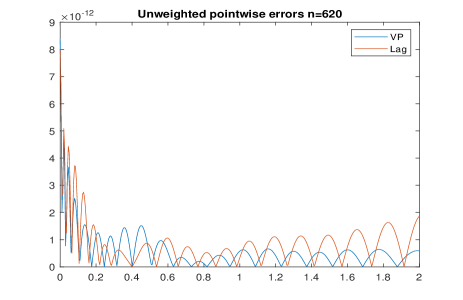
Figure 2: Example 1: Plots of $\tilde{e}^{VP}_{n,m}(f_{1},x)$ and $\tilde{e}^{Lag}_{n+1}(f_{1},x)$ for $n=620$, $m=186$.

Example 2

Consider

$$\alpha=0.5,\quad\gamma=0.5\quad f_{2}(x)=\frac{|x-1|^{\frac{11}{2}}}{100+x^{2}}$$

In this case, $f_{2}$ belongs to an intermediate space between $W_{1}(u)$ and $W_{2}(u)$. According to [5, (5.2.7)], the theoretical convergence order is $\mathcal{O}\left(\frac{1}{(n-m)^{\frac{11}{4}}}\right)$ for $\mathcal{E}_{n,m}^{VP}$, and $\mathcal{O}\left(\frac{\log N}{N^{\frac{11}{4}}}\right)$ for $\mathcal{E}_{N}^{Lag}$. As shown in Table 2, all the numerical errors agree with the theoretical estimates and are comparable as a consequence of the very slow divergence of the logarithmic factor. In particular, VP approximation provides a slightly better approximation than the interpolating polynomial in the case $N=n$. This trend is little bit reversed when $N=n+m$.

However, in Figure 3, the graphics of the pointwise error function taken for $n=420,\ m=126$, shows that $V_{n}^{m}(w_{\alpha},f_{2})$ provides a pointwise approximation better than the one offered by $L_{n+1}^{*}(w_{\alpha},f_{2})$.

$n$	$m$	# f.eval	$\mathcal{E}_{n,m}^{VP}$	$\mathcal{E}_{n}^{Lag}$	# f.eval	$\mathcal{E}_{n+m}^{Lag}$
20	6	19	1.10e-04	4.17e-02	25	2.92e-02
220	22	96	9.78e-08	9.23e-08	101	5.17e-08
420	42	134	1.27e-08	1.38e-08	140	8.54e-09
620	310	163	1.54e-09	2.36e-09	200	1.42e-09
820	82	188	2.47e-09	2.53e-09	197	1.63e-09
1020	102	210	1.31e-09	1.31e-09	220	1.01e-09
1220	122	230	7.28e-10	7.39e-10	241	5.75e-10

Table 2: Maxima weighted errors induced by interpolating and VP polynomials for Example 2.

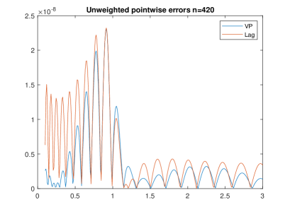
Figure 3: Example 2: Plots of $\tilde{e}^{VP}_{n,m}(f_{2},x)$ and $\tilde{e}^{Lag}_{n+1}(f_{2},x)$ for $n=420$, $m=126$.

Example 3

Consider the case

$$f_{3}(x)=\frac{1}{1+100(x-3)^{2}},\quad\alpha=-0.4,\quad\gamma=0.05\quad$$

$n$	$m$	# f.eval	$\mathcal{E}_{n,m}^{VP}$	$\mathcal{E}_{n}^{Lag}$	# f.eval	$\mathcal{E}_{n+m}^{Lag}$
20	6	17	2.24e-01	2.25e-01	20	1.13e-01
220	22	64	9.04e-02	8.95e-02	67	1.57e-01
420	378	89	6.98e-02	8.34e-02	123	8.31e-02
620	558	108	6.21e-02	7.05e-02	149	4.12e-02
820	738	124	3.72e-02	4.93e-02	172	2.56e-02
1020	102	139	5.86e-02	5.82e-02	146	5.66e-02
1220	1098	152	2.84e-02	3.64e-02	209	2.87e-02

Table 3: Maxima weighted errors induced by interpolating and VP polynomials for Example 3.

Note that $f_{3}\in W_{r}(u)$, $\forall r>0$, and the slow convergence we see in Table 3 depends on the growth of the norms in the error estimates. For instance, with $r=5$, $\|f_{3}\|_{W_{5}(u)}\sim 0.5e+12$. Similarly to the previous example, the maxima errors attained by VP and Lagrange approximation are almost comparable among them. However, also in this case in Figure 4 are displayed the absolute pointwise errors taken for $n=420,\ m=378$, and except a small range around the peak point $x=3$, the errors by $V_{n}^{m}(w_{\alpha},f)$ are smaller than those by $L_{n+1}^{*}(w_{\alpha},f)$.

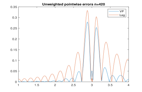
Figure 4: Example 3: Plots of $\tilde{e}^{VP}_{n,m}(f_{3},x)$ and $\tilde{e}^{Lag}_{n+1}(f_{3},x)$ for $n=420$ and $m=378$

Example 4

Let be

$$\alpha=0.6,\quad\gamma=0.6\quad f_{4}(x)=|\cos(\pi-x)|$$

$n$	$m$	# f.eval	$\mathcal{E}_{n,m}^{VP}$	$\mathcal{E}_{n}^{Lag}$	# f.eval	$\mathcal{E}_{n+m}^{Lag}$
20	2	19	1.37e-01	1.36e-01	21	1.16e-01
220	22	79	3.24e-02	3.25e-02	83	3.95e-02
420	84	108	2.57e-02	2.63e-02	121	1.65e-02
620	62	137	1.75e-02	1.73e-02	141	1.23e-02
820	82	155	1.69e-02	1.67e-02	152	1.63e-02
1020	102	173	1.76e-02	1.74e-02	182	1.25e-02
1220	488	190	8.31e-03	8.01e-03	225	9.35e-03

Table 4: Maxima weighted errors induced by interpolating and VP polynomials for Example 4.

In this case we have $f_{4}\in W_{1}(u)$, and the degree of approximation is very poor, since, according to (2), VP and Lagrange approximation rates are $\mathcal{O}\left(\frac{1}{\sqrt{n-m}}\right),\mathcal{O}\left(\frac{\log n}{\sqrt{n}}\right)$, respectively. The numerical results displayed in Table 4 and Figure 5 agree with the theory and, as the previous cases, we see that the maxima errors are almost comparable but, concerning the local approximation, VP approximation error behaves better away from the singularity $x=\pi/2$.

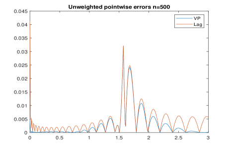
Figure 5: Example 4: Plots of $\tilde{e}^{VP}_{n,m}(f_{3},x)$ and $\tilde{e}^{Lag}_{n+1}(f_{3},x)$ for $n=500$ and $m=150$.

Example 5

Now consider the following function plotted in Figure 6 (left–hand side)

$$f(x)=\frac{1}{1+100(x-0.5)^{2}}+\frac{1}{1+1000\sqrt{x^{2}+0.5}},\quad\gamma=0.5$$

To evidence the improvement in the pointwise approximation achieved by VP polynomials, on the right–hand side of Fig. 6 we report the plots of both Lagrange and VP polynomials when $n=400$, $\alpha=0$ and $m=200.$

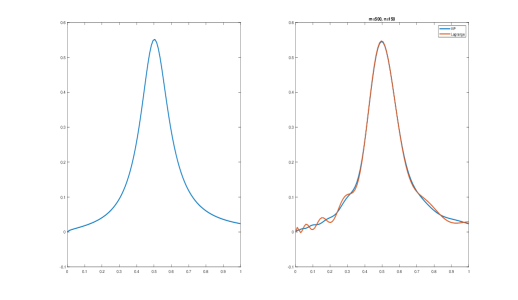
Figure 6: Example 5: graphic of the function $f_{5}$ (left) and plots of the VP and Lagrange polynomials (right) for $\alpha=0$, $n=400$ and $m=200.$

Example 6

This test highlights the feature offered by VP polynomials when we want to approximate functions of bounded variation having a jump discontinuity. Consider the function

$$f_{6}(x)=\begin{cases}x,&x<1\\ x+2,&x\geq 1\end{cases}$$

Figure 7 displays the graphics of $f_{6}u$ with $u(x)=e^{-\frac{x}{2}}\sqrt{x}$ (black line) and the approximations by the weighted Lagrange polynomial $uL_{n+1}^{*}(w_{\alpha},f_{6})$ (orange line) and the weighted $uV_{n}^{m}(w_{\alpha},f_{6})$ (blue line), for $n=620$ and $m=310$.

As expected, the Gibbs phenomenon appears. In fact, as the graphics in Figure 7 show, the Lagrange polynomial presents damped oscillations that persist even when moving away from the jump while the VP polynomial induces a reduction of the Gibbs phenomenon as $m$ increases. This is confirmed by Figure 8 displaying the unweighted absolute error induced by Lagrange polynomial and VP polynomial

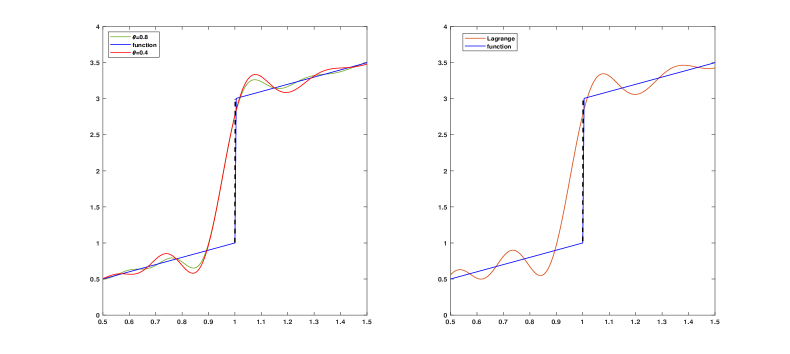
Figure 7: $n=620$, $\alpha=0.5$, $\gamma=0.5$: the function $f_{6}u$ and weighted VP polynomials for $m=298$, $m=496$ (left), and the weighted Lagrange polynomial of degree $n$ (right).

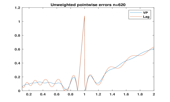
Figure 8: $n=620$, $m=310$, $\alpha=0.5$.

4.2 Behavior of the weighted Lebesgue constants

In what follows we show the behavior of the Lebesgue constants related to Lagrange and VP approximation for different choices of $\alpha$ and $\gamma$, as $n$ increases. From the theory sufficient conditions relating $\alpha$ and $\gamma$ are known to ensure the optimal logarithmic grow in the Lagrange case (cf. (8)), and the uniform boundedness in the VP case (cf. (26)). In the latter case, it is also required that $m\approx n$ to get a near best approximation order. To this aim, we take $m=\lfloor n\theta\rfloor$, being $\theta\in(0,1)$ chosen as $\theta\in\{0.1,0.2,\dots,0.9.\}$. Hence for these values of $\theta$ and $n$ increasing, the behavior of the Lebesgue constants is displayed in Figures 9-10 for several couples of $(\alpha,\gamma)$ both in the ranges to obtain optimal Lebesgue constants for VP and Lagrange operators.

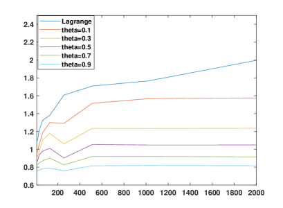
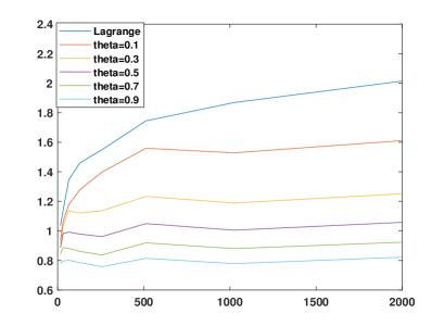
Figure 9: Lebesgue constants for $\alpha=\gamma=0.5$ (left), for for $\alpha=\gamma=1$ (right).

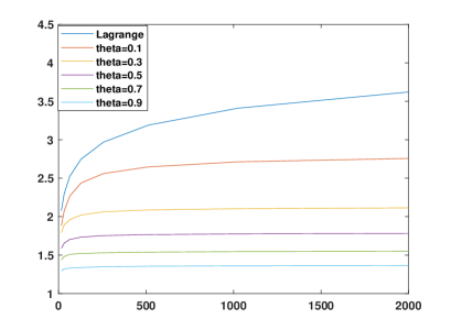
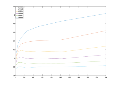
Figure 10: Lebesgue constants for $\alpha=-0.5,\gamma=0$ (left), $\alpha=0.7,\gamma=0.6$ (right).

In conclusion, in Figure 11 we consider the case when $\alpha$ and $\gamma$ do not satisfy the bounds in (26) concerning VP approximation, but they satisfy those in (8) concerning Lagrange. In this case, even if not predicted by Theorem 3.1 we see the Lebesgue constants of VP operator are still bounded for any $\theta$.

Empirically we have detected that the same behavior occurs for other possible choices of couples of $(\alpha,\gamma)$ s.t. $\frac{\alpha}{2}+\frac{7}{6}<\gamma\leq\frac{\alpha}{2}+\frac{5}{4}.$ This observation leads us to conjecture that the hypotheses of Theorem 3.1 can be extended by replacing the upper bound $\min\{\frac{\alpha}{2}+\frac{7}{6},\alpha+1\}$ by $\frac{\alpha}{2}+\frac{5}{4}$.

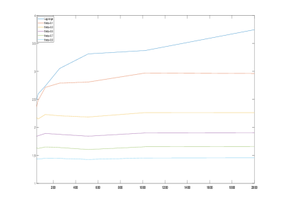
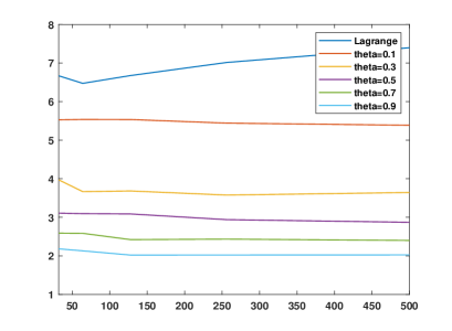
Figure 11: Lebesgue constants for $\alpha=0.5,\gamma=1.43$ (left), $\alpha=0,\gamma=5/4$ (right).

5 Conclusions

We have introduced and studied a new truncated polynomial operator $V_{n}^{m}(w_{\alpha}):C_{u}\to C_{u}$, involving the values of $f$ at only the first $j<<n$ zeros of the Laguerre polynomial $p_{n}(w_{\alpha})$. Differently from $L_{n+1}^{*}(w_{\alpha})$, we have proved that the map $V_{n}^{m}(w_{\alpha}):C_{u}\to C_{u}$ is uniformly bounded under suitable conditions on the weights $w_{\alpha}$ and $u$ and in view of this theoretical improvement, the maxima errors attained by VP approximation are better on average than those achieved by Lagrange one. However, the differences between the numerical errors in norm are not so large, since the factor $\log n$ does not have a strong impact in the error estimate. The situation is instead quite different about the pointwise errors, especially in approximating smooth functions presenting some peaks or isolated pathologies (see Examples 4-5). Indeed, in such cases the additional parameter $m$ can be suitably modulated to reduce the Gibbs phenomenon. We observe a drastic reduction of the oscillations in VP polynomials as $m$ increases, and even more w.r.t the Lagrange polynomial, the latter swinging more than anyone. Such reduction is valuable also in Example 6 where $f_{6}$ is a bounded variation function. In these cases it is well–known that Lagrange polynomials present overshoots and oscillations not only close to the singularities, but also in the smooth part of the function. The graphics in Fig. 7 show how the Gibbs phenomenon can be reduced by VP polynomials, for suitable values of the parameter $\theta\in(0,1).$ We conclude observing that the range where $\alpha,\gamma$ vary for the boundedness of VP polynomials, is partially overlapping with that the norm of the Lagrange operator logarithmically behaves (compare (8) and (26)), and in any case the VP range is larger than the Lagrange one. However, numerical results (see Fig. 11) allow us to conjecture that the range determined by Thm. 3.1 about the parameters $\alpha,\gamma$ could actually be stretched. More precisely, we conjecture that the hypothesis $\max\{0,\frac{\alpha}{2}-\frac{1}{4}\}<\gamma\leq\frac{\alpha}{2}+\frac{5}{4}$ could replace (26).

Acknowledgments. This work was partially supported by INdAM-GNCS. The research has been accomplished within RITA (Research ITalian network on Approximation)

References

[1]
M. C. De Bonis, G. Mastroianni, and M. Viggiano.
K-functionals, moduli of smoothness and weighted best approximation
on the semiaxis.
1999.
[2]
Mhaskar H. N. and E. B. Saff.
Extremal problems for polynomials with Laguerre weights.
Approx. Theory IV, Academic Press, 1983.
[3]
C. Laurita and G. Mastroianni.
Lp-convergence of lagrange interpolation on the semiaxis.
Acta Math. Hungar, 120(3):249–273, 2008.
[4]
G. Mastroianni.
Polynomial inequalities, functional spaces and best approximation on
the real semiaxis with laguerre weights.
Electronic Transactions on Numerical Analysis, 14:142–151,
2002.
[5]
G. Mastroianni and G. V. Milovanovic.
Interpolation Processes Basic Theory and Applications.
Springer Monographs in Mathematics. Springer Verlag, Berlin, 2009.
[6]
G. Mastroianni and G. V. Milovanovi.̧
Some numerical methods for second-kind Fredholm integral equations
on the real semiaxis.
IMA Journal of Numerical Analysis, 29(4):1046–1066, 2009.
[7]
G. Mastroianni and G. Monegato.
Truncated quadrature rules over and Nyström-type
methods.
SIAM Journal on Numerical Analysis, 41:1870 –1892, 2003.
[8]
G. Mastroianni and I. Notarangelo.
Some fourier-type operators for functions on unbounded intervals.
Acta Math. Hungar., 127((4)):347 –375, 2010.
[9]
G. Mastroianni and D. Occorsio.
Lagrange interpolation at Laguerre zeros in some weighted uniform
spaces.
Acta Math. Hungar., 91((1-2)):27–52, 2001.
[10]
G. Mastroianni and D. Occorsio.
Some quadrature formulae with nonstandard weights.
Jour. of Comput. and Appl. Math., 235:602–614, 2010.
[11]
G. Mastroianni and J. Szabados.
Polynomial approximation on infinite intervals with weights having
inner zeros.
Acta Math. Hungar, 96(3):221–258, 2002.
[12]
G. Mastroianni and J. Szabados.
Direct and converse polynomial approximation theorems on the real
line with weights having zeros,.
volume 283 of Pure Appl. Math. (Boca Raton), pages 287–306.
2007.
[13]
G. Mastroianni and W. Themistoclakis.
Uniform approximation on via discrete de la vallée poussin
means.
Acta Sci. Math., 74:147–170, 2008.
[14]
G. Mastroianni and W. Themistoclakis.
Pointwise estimates for polynomial approximation on the semiaxis.
Jour. of Approx. Theory, 162(11):2078–2105, 2010.
[15]
G. Mastroianni and P. Vértesi.
Fourier sums and lagrange interpolation on and
.
volume 283 of Pure Appl. Math. (Boca Raton), pages 307–344.
2007.
[16]
E. Poiani.
Mean Cesàro summability of Laguerre and hermite series.
Transactions of the American Mathematical Society, 1972.
[17]
G. Szegö.
Orthogonal Polynomials, volume 4th Ed.
American Mathematical Society, Providence, RI, 1975.
[18]
W. Themistoclakis.
Uniform approximation on via discrete de la vallée poussin
means.
Numer. Alg., 60:593–612, 2012.