Azimuthal metallicity variations, spiral structure, and the failure of radial actions based on assuming axisymmetry

Abstract

We study azimuthal variations in the mean stellar metallicity, $\left<{\mbox{$\rm[Fe/H]$}}\right>$, in a self-consistent, isolated simulation in which all stars form out of gas. We find $\left<{\mbox{$\rm[Fe/H]$}}\right>$ variations comparable to those observed in the Milky Way and which are coincident with the spiral density waves. The azimuthal variations are present in young and old stars and therefore are not a result of recently formed stars. Similar variations are present in the mean age and $\rm\alpha$-abundance. We measure the pattern speeds of the $\left<{\mbox{$\rm[Fe/H]$}}\right>$-variations and find that they match those of the spirals, indicating that they are at the origin of the metallicity patterns. Because younger stellar populations are not just more $\rm[Fe/H]$-rich and $\rm\alpha$-poor but also dynamically cooler, we expect them to more strongly support spirals, which is indeed the case in the simulation. However, if we measure the radial action, $J_{R}$, using the Stäckel axisymmetric approximation, we find that the spiral ridges are traced by regions of high $J_{R}$, contrary to expectations. Assuming that the passage of stars through the spirals leads to unphysical variations in the measured $J_{R}$, we obtain an improved estimate of $J_{R}$ by averaging over a $1\mbox{$\>{\rm Gyr}$}$ time interval. This time-averaged $J_{R}$ is a much better tracer of the spiral structure, with minima at the spiral ridges. We conclude that the errors incurred by the axisymmetric approximation introduce correlated deviations large enough to render the instantaneous radial actions inadequate for tracing spirals.

1 Introduction

Observations of Milky Way (MW) disc stars have been finding azimuthal variations in the mean stellar metallicity at fixed radius. Early work using small samples of Cepheids, which are less than $1\mbox{$\>{\rm Gyr}$}$ old, found an azimuthal variation in the metallicity at the Solar radius (Luck et al., 2006). On a larger scale, Pedicelli et al. (2009) showed that the relative abundance of metal-rich and metal-poor Cepheids varies across the different quadrants. While Luck et al. (2011) were unable to detect any azimuthal metallicity variations in a sample of 101 Cepheids, Lépine et al. (2011) found azimuthal variations in both Cepheids and open clusters comparable to the radial gradient, and attributed them to the spiral structure.

Large surveys, such as APOGEE and the Gaia data releases (Majewski et al., 2016; Gaia Collaboration et al., 2018) have significantly accelerated the characterisation of azimuthal stellar metallicity variations. Bovy et al. (2014) used a $\sim 10^{4}$ red clump star sample from APOGEE, with an age distribution favouring $1-4\mbox{$\>{\rm Gyr}$}$, to search for azimuthal metallicity variations. They found azimuthal variations to be smaller than $0.02$ dex within an azimuthal volume spanning $45^{\circ}$. Poggio et al. (2022) used Gaia DR3 data to map metallicity variations within $4\mbox{$\>{\rm kpc}$}$ of the Sun. They showed that metal-rich stars trace the spiral structure. They also found that these variations are stronger for young stars, but are also present in old stellar populations. Hawkins (2023) used a sample of OBAF stars from LAMOST, and a separate sample of giant stars from Gaia DR3 to measure radial and vertical metallicity gradients. He also found azimuthal metallicity variations of order $\sim 0.1$ dex on average, which are co-located with the spiral structure in the Gaia data (but not in the LAMOST data). Imig et al. (2023) used 66K APOGEE DR17 red giants to suggest that the azimuthal metallicity variations in the Solar Neighbourhood do not seem to track the spiral structure.

Theoretical studies of azimuthal metallicity variations attribute them to spiral structure, via a number of different mechanisms. The simplest idea is that the metallicity variations reflect the higher metallicity of recently formed stars, since the gas metallicity itself has an azimuthal variation of $\sim 0.1$ dex (Wenger et al., 2019). Comparable variations in gas metallicity have also been found in external galaxies (e.g. Sánchez-Menguiano et al., 2016; Vogt et al., 2017; Ho et al., 2018; Kreckel et al., 2019; Hwang et al., 2019). Spitoni et al. (2019) developed a chemical evolution model of the Galactic disc perturbed by a spiral. They found large metallicity variations near the corotation of the spiral. Solar et al. (2020) measured the metallicity of star-forming regions in EAGLE (Schaye et al., 2015) simulated galaxies finding variations of $\sim 0.12$ dex. Bellardini et al. (2022) used a suite of FIRE-2 cosmological simulations (Hopkins et al., 2018) to show that the azimuthal variation in the stellar metallicity at birth decreases with time, mirroring the evolution of the gas phase metallicity (Bellardini et al., 2021).

Alternatively, azimuthal variations of the mean stellar metallicity have been viewed as a signature of radial migration. Using an $N$-body simulation of a barred spiral galaxy, in which star particles had metallicity painted on based on their initial radius, Di Matteo et al. (2013) proposed that azimuthal metallicity variations are produced by the radial migration induced by the non-axisymmetric structure. Meanwhile, in a zoom-in cosmological simulation, Grand et al. (2016b) found that the kinematic motions induced by the spirals drive an azimuthal variation in the metallicity, with metal-rich stars on the trailing side and metal-poor ones on the leading side, which they interpreted as a signature of migration of stars from a stellar disc with a radial metallicity gradient. Carr et al. (2022) noted that, in high-resolution $N$ body simulations (Laporte et al., 2018) of the Sagittarius dwarf’s encounter with the Milky Way, azimuthal metallicity variations appear in the disc’s impulsive response to the passage through the disc, during which migration is also enhanced, and then continuing within the spirals in the periods between passages.

A third hypothesis on the origin of azimuthal metallicity variations posits that they are produced by the different reactions of different stellar populations to a spiral perturbation. Khoperskov et al. (2018) used pure $N$-body (no gas or star formation) simulations of compound stellar discs to show that azimuthal variations can be produced by the varying response of cool, warm and hot stellar populations to spirals. Even in the absence of a metallicity gradient in the disc, if the different populations have different metallicities, azimuthal variations result. They showed that, when migration dominates the azimuthal variations (because all populations had the same radial metallicity profile), the metallicity and density peaks are offset, whereas when the variations are driven by the different response of different populations then the density and metallicity peaks tend to align.

In this paper we explore the link between spiral structure and azimuthal metallicity variations. In agreement with Khoperskov et al. (2018), we show, using a model with star formation and self-consistent chemical evolution, that the main driver of these variations are differences in how strongly a stellar population can trace the spiral structure based on its radial action. In Section 2 we describe the simulation used in this paper. In Section 3 we describe the azimuthal chemical variations, both for $\rm[Fe/H]$ and $\rm[O/Fe]$. We find that variations in the average $\rm[Fe/H]$ closely track the spiral structure. Therefore in Section 4 we construct a method to track the pattern speeds of the average metallicity variations, taking care to ensure that the average metallicity is not weighted by the density. Thus the pattern speeds of the metallicity variations we obtain are independent from those of the density. We show that there is such a close correspondence between the pattern speeds of the average metallicity and of the density in the disc region that it must be the spirals that are driving the metallicity variations. Section 5 explores the idea that the metallicity variations are due to young stars but finds that the azimuthal metallicity variations are present in all age populations, both very young and those older than $6\mbox{$\>{\rm Gyr}$}$. Then in Section 6 we explore the dependence on the radial action. We find that the radial action provides a very robust explanation for the azimuthal metallicity variations, provided that the radial action is time averaged to reduce the errors introduced by the assumption of axisymmetry. We show that instantaneous values of the radial action instead provide almost exactly the wrong answer, in that stars with seemingly large radial action trace the spiral. We present our conclusions in Section 8.

2 Simulation description

The model we use here was first described in Fiteni et al. (2021), who referred to it as model M1_c_b. The model evolves via the cooling of a hot gas corona, in equilibrium within a spherical dark matter halo. The dark matter halo has a virial mass $M_{200}=10^{12}\>{\rm M_{\odot}}$ and a virial radius $r_{200}\simeq 200~{}\mbox{$\>{\rm kpc}$}$, making it comparable to the MW (see the review of Bland-Hawthorn & Gerhard, 2016, and references therein). The gas corona has the same profile but with an overall mass that is $10\%$ that of the dark matter. The initial gas corona, as well as the dark matter halo, is comprised of 5 million particles, which means gas particles have an initial mass of $2.8\times 10^{4}\>{\rm M_{\odot}}$. The dark matter particles come in two mass species, one of mass $2\times 10^{5}\>{\rm M_{\odot}}$ inside $r=200\mbox{$\>{\rm kpc}$}$ and the other of mass $7.1\times 10^{5}\>{\rm M_{\odot}}$ outside. Gas particles are softened with $\varepsilon=50~{}\mbox{$\>{\rm pc}$}$, while the dark matter particles have $\varepsilon=100~{}\mbox{$\>{\rm pc}$}$. A cylindrical spin is imparted to the gas particles such that the gas corona has $\lambda\equiv L|E|^{1/2}/(GM_{vir}^{5/2})=0.065$, where $L$ and $E$ are the total angular momentum and energy of the gas, and $G$ is the gravitational constant (Peebles, 1969). After setting up the system, we evolve it adiabatically for $5\mbox{$\>{\rm Gyr}$}$ without gas cooling or star formation to ensure that it is fully relaxed.

We then evolve these initial conditions with gas cooling and star formation. As the gas cools, it settles into a rotationally supported disc and ignites star formation. Thus all stars form directly out of gas. Individual star particles inherit their softening, $\varepsilon=50~{}\mbox{$\>{\rm pc}$}$, and chemistry from the gas particle from which they form. Star formation, with an efficiency of 5 per cent, requires a gas particle to have cooled below 15,000 K, exceeded a density of $0.1$ amu cm^-3 and to be part of a convergent flow. Star particles are all born with the same mass, $9.3\times 10^{3}\>{\rm M_{\odot}}$, which is $1/3$ of the (initial) gas particle mass. Gas particles continue to form stars until their mass falls below $5.6\times 10^{3}\>{\rm M_{\odot}}$ ($20\%$ of the initial gas particle mass), at which point a gas particle is removed and its mass distributed to the nearest gas particles. After $13\mbox{$\>{\rm Gyr}$}$, roughly $2.6$ million gas particles remain.

Once star formation begins, feedback from supernovae Ia and II, and from AGB winds, couples $4\times 10^{51}$ erg per supernova to the interstellar medium using the blastwave prescription of Stinson et al. (2006). Thermal energy and chemical elements are mixed amongst gas particles using the turbulent diffusion prescription of Shen et al. (2010) with a mixing coefficient of 0.03.

The model is evolved for $13\mbox{$\>{\rm Gyr}$}$ with gasoline (Wadsley et al., 2004, 2017), an $N$-body$+$SPH code. Gravity is solved using a KD-tree; we employ a tree opening angle of $\theta=0.7$ with a base time-step of $\Delta t=5\mbox{$\>{\rm Myr}$}$. Time-steps of individual particles are then refined by multiples of 2 until they satisfy the condition $\delta t\equiv\Delta t/2^{n}<\eta\sqrt{\varepsilon/a_{g}}$, where $a_{g}$ is the gravitational acceleration of a particle, and we set the refinement parameter $\eta=0.175$. Time-steps for gas particles are also refined in a similar manner to satisfy the additional condition $\delta t_{gas}<\eta_{courant}h/[(1+\alpha)c+\beta\mu_{max}]$, where $\eta_{courant}=0.4$, $h$ is the SPH smoothing length set over the nearest 32 particles, $\alpha=1$ is the shear coefficient, $\beta=2$ is the viscosity coefficient, $c$ is the sound speed and $\mu_{max}$ is the maximum viscous force between gas particles (Wadsley et al., 2004). With these time stepping recipes, typically 10 rungs (maximum $n=9$, corresponding to $\delta t=9766\mbox{$\>{\rm yr}$}$) are required to move all the particles.

We save snapshots of the simulation every $5\mbox{$\>{\rm Myr}$}$. This high cadence gives a Nyquist frequency of $\sim 300\mbox{$\>{\rm km\,s^{-1}\,kpc^{-1}}$}$ (for $m=2$ perturbations), which is well above any frequency of interest in our MW-sized galaxy. By $t=13~{}\mbox{$\>{\rm Gyr}$}$, which is the main snapshot we consider here, the simulation has formed 11,587,120 star particles, allowing us to dissect the model by stellar population properties while ensuring that we have enough particles for reliable study.

Fiteni et al. (2021) showed that this model experiences an episode of mild clump formation lasting to $\sim 2\mbox{$\>{\rm Gyr}$}$, which gives rise to a small population of retrograde stars in the Solar Neighbourhood. A bar also forms at $t\simeq 4~{}\mbox{$\>{\rm Gyr}$}$, which subsequently weakens at $t\simeq 7\mbox{$\>{\rm Gyr}$}$ before recovering. Meanwhile, Khachaturyants et al. (2022a) showed that weak bending waves propagate through the disc, with peak amplitudes $\la 50~{}\mbox{$\>{\rm pc}$}$ in the Solar Neighbourhood. Khachaturyants et al. (2022b) computed the pattern speeds of the density perturbations (bar$+$spirals), as well as those of the breathing and bending waves in this model. They showed that the breathing waves have the same pattern speeds as the spirals and bar, but very different pattern speeds from the bending waves, from which they concluded that breathing waves are driven by density perturbations. Finally Ghosh et al. (2022) used this model at $12\mbox{$\>{\rm Gyr}$}$ to show that breathing motions induced by spirals get larger with distance from the mid-plane, and are stronger for younger stars than for older stars.

We focus most of our analysis on the single snapshot of this model at $t=13\mbox{$\>{\rm Gyr}$}$. We have verified that results are broadly similar at other times, and in the appendix we present the azimuthal metallicity variations at other times.

3 Chemical azimuthal variations

3.1 The azimuthal variation of $\left<{\mbox{$\rm[Fe/H]$}}\right>$

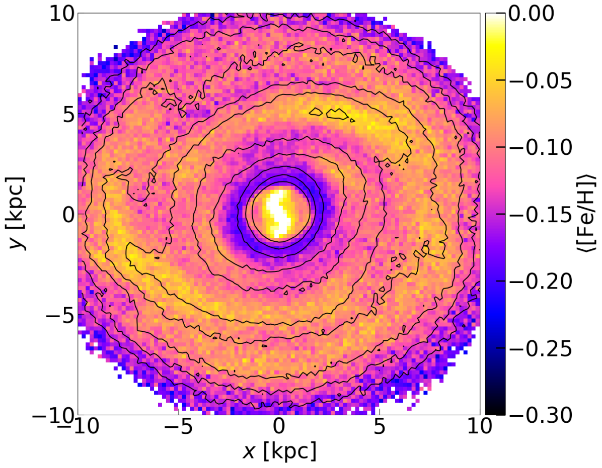
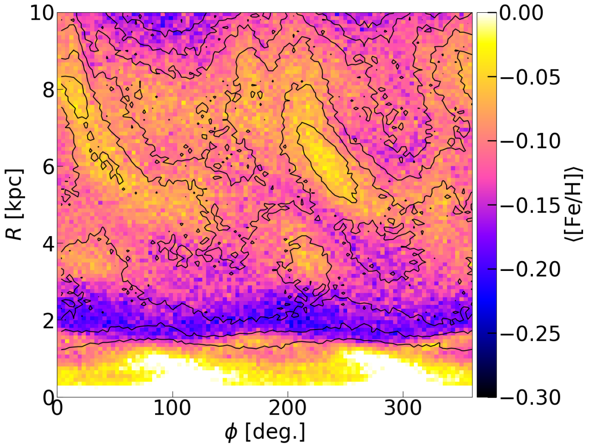
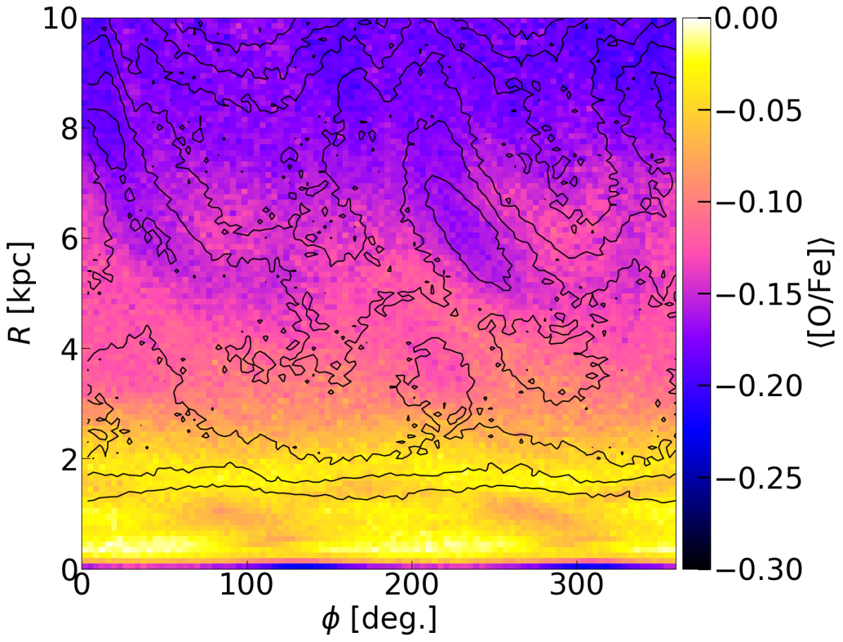
Figure 1: Top: $\left<{\mbox{$\rm[Fe/H]$}}\right>$ in Cartesian, $(x,y)$, and middle: cylindrical, $(R,\phi)$, coordinates. The bottom panel shows $\left<{\mbox{$\rm[O/Fe]$}}\right>$ in cylindrical coordinates. In all panels the contours correspond to the surface density. The disc is rotating in a counter-clockwise sense, i.e. rotation is in the direction of increasing $\phi$. The model is shown at $13~{}\mbox{$\>{\rm Gyr}$}$.

In Fig. 1 we present the mean metallicity, $\left<{\mbox{$\rm[Fe/H]$}}\right>$, of the model at $13~{}\mbox{$\>{\rm Gyr}$}$ in both Cartesian (top) and cylindrical (middle) coordinates. Clear azimuthal variations in $\left<{\mbox{$\rm[Fe/H]$}}\right>$ are present. The density contours show a weak bar extending to $R\sim 2~{}\mbox{$\>{\rm kpc}$}$ and open spirals beyond. In the disc region ($R>5\mbox{$\>{\rm kpc}$}$), the peak $\left<{\mbox{$\rm[Fe/H]$}}\right>$ coincides with regions of high density on the spirals.

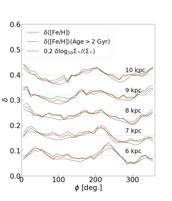
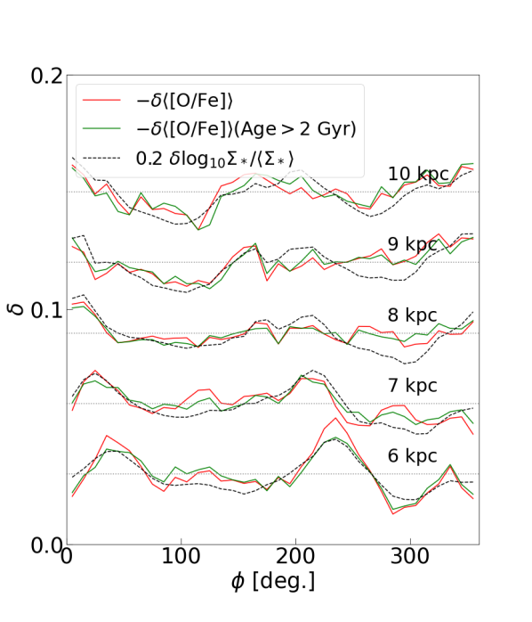
Figure 2: The variation of $\left<{\mbox{$\rm[Fe/H]$}}\right>$ (left) and $-\mbox{$\left<{\mbox{$\rm[O/Fe]$}}\right>$}$ (right) compared with the density variation at a series of $500~{}\mbox{$\>{\rm pc}$}$-wide annuli centred at $6\mbox{$\>{\rm kpc}$}$ to $10\mbox{$\>{\rm kpc}$}$, as indicated. The average values for each radius are subtracted from each azimuthal profile and the profiles are then vertically offset by a fixed amount to show the variation. The azimuthal profiles of the density have been scaled by the indicated factors for ease of comparison. The dotted horizontal lines indicate the zero for each radius.

The left panel of Fig. 2 compares the azimuthal variations of the stellar surface density, $\delta\Sigma/\mbox{$\left<{\Sigma}\right>$}$, with those of the mean metallicity, $\delta\mbox{$\left<{\mbox{$\rm[Fe/H]$}}\right>$}$, in the disc region. At these radii ($5.75\leq R/\mbox{$\>{\rm kpc}$}\leq 10.25$), where the spirals dominate, the variations in $\left<{\mbox{$\rm[Fe/H]$}}\right>$ closely follow those of the density, with peaks and troughs at the same locations. This panel also shows that the $\delta\mbox{$\left<{\mbox{$\rm[Fe/H]$}}\right>$}$ of stars older than $2\mbox{$\>{\rm Gyr}$}$ behaves very similarly to that of the full distribution, with only slightly weaker amplitudes, indicating that recent metal-rich star formation is not driving the $\left<{\mbox{$\rm[Fe/H]$}}\right>$ variations. The main variation in both the density and $\left<{\mbox{$\rm[Fe/H]$}}\right>$ has an $m=2$ multiplicity. The maximum to minimum variations in $\left<{\mbox{$\rm[Fe/H]$}}\right>$ are of order $0.05-0.1$ dex outside the bar radius. In the MW, Hawkins (2023) found metallicity variations of the same order.

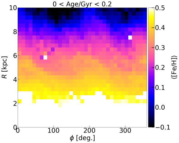
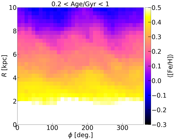
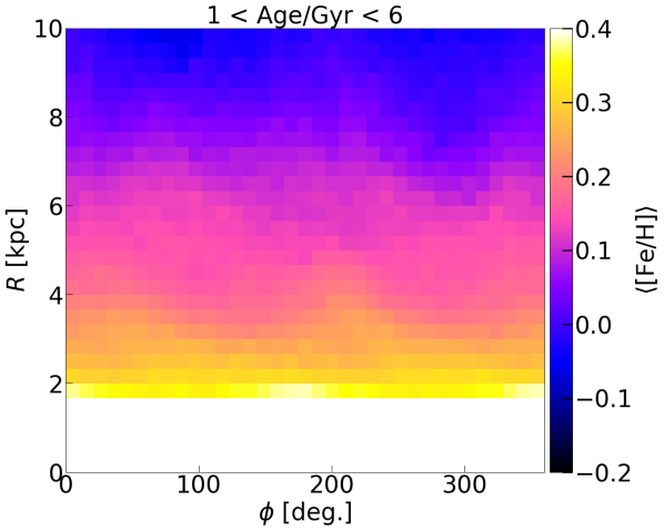
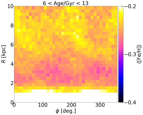
Figure 3: The distribution of stellar $\left<{\mbox{$\rm[Fe/H]$}}\right>$ at $13\mbox{$\>{\rm Gyr}$}$ split by age, as indicated. White represents bins with $\left<{\mbox{$\rm[Fe/H]$}}\right>$ off the scale (inside $\sim 2\mbox{$\>{\rm kpc}$}$) or with less than 10 particles (elsewhere).

Since the azimuthal variations in $\left<{\mbox{$\rm[Fe/H]$}}\right>$ are not limited to the young stars, we proceed by exploring the $\left<{\mbox{$\rm[Fe/H]$}}\right>$-azimuthal variations of different age populations. Fig. 3 shows $\left<{\mbox{$\rm[Fe/H]$}}\right>$ in cylindrical coordinates for four age groups. A clear azimuthal variation is present in the very young ($\mbox{$\tau$}\leq 200$ $\>{\rm Myr}$) stars, as seen in the MW (Luck et al., 2006; Lemasle et al., 2008; Pedicelli et al., 2009). A similar pattern is seen in slightly older stars, up to $1\mbox{$\>{\rm Gyr}$}$ old. This behaviour might be expected if the spirals are the locii of metal-rich star formation. But a similar azimuthal variation in $\left<{\mbox{$\rm[Fe/H]$}}\right>$ is evident in the intermediate age stars ($1<\mbox{$\tau$}/\mbox{$\>{\rm Gyr}$}<6$) and even, to a lesser extent, in the old stars ($6<\mbox{$\tau$}/\mbox{$\>{\rm Gyr}$}<13$). Thus the azimuthal variation of $\left<{\mbox{$\rm[Fe/H]$}}\right>$ is not a result of recent star formation but must be inherent to spiral structure.

From the observations that the $\left<{\mbox{$\rm[Fe/H]$}}\right>$ peaks are radially extended but coincident with the density peaks, we conclude that the cause of the $\left<{\mbox{$\rm[Fe/H]$}}\right>$ variations is unlikely to be a resonant phenomenon, since azimuthal variations due to stars librating about a resonance might be expected to have $\rm[Fe/H]$ peaks azimuthally displaced relative to the perturbation (e.g. Grand et al., 2016b; Khoperskov et al., 2018).

3.2 The azimuthal variation of $\left<{\mbox{$\rm[O/Fe]$}}\right>$

The simulation also tracks the evolution of $\rm[O/Fe]$; the bottom panel of Fig. 1 shows the azimuthal variation of $\left<{\mbox{$\rm[O/Fe]$}}\right>$ at $13\mbox{$\>{\rm Gyr}$}$. We find very similar behaviour as for $\left<{\mbox{$\rm[Fe/H]$}}\right>$, but since $\rm[Fe/H]$ and $\rm[O/Fe]$ are anti-correlated, the minima in $\left<{\mbox{$\rm[O/Fe]$}}\right>$ are at the density peaks.

The right panel of Fig. 2 compares the azimuthal variations of $\left<{\mbox{$\rm[O/Fe]$}}\right>$ with those of the density (with a minus sign on $\left<{\mbox{$\rm[O/Fe]$}}\right>$ so maxima and minima are aligned). The peak to trough variation is of order $0.03$ at small radii declining at larger radii. Overall a match in location of the peaks and troughs is present but the correspondence is somewhat less exact than between $\left<{\mbox{$\rm[Fe/H]$}}\right>$ and $\delta\Sigma/\mbox{$\left<{\Sigma}\right>$}$.

4 Pattern speeds

Having shown the close correspondence between spirals and $\left<{\mbox{$\rm[Fe/H]$}}\right>$ variations at one time, we explore their co-evolution across time by treating the $\left<{\mbox{$\rm[Fe/H]$}}\right>$ variations as waves, and comparing their pattern speeds with those of the spirals. We use the spectral analysis code of Khachaturyants et al. (2022b), which uses binned data to measure pattern speeds. We bin the mass and $\rm[Fe/H]$ data in polar coordinates with $R\in[0,12]\mbox{$\>{\rm kpc}$}$ and $\Delta R=0.5\mbox{$\>{\rm kpc}$}$, and $\varphi\in[0,360]^{\circ}$ and $\Delta\varphi=10^{\circ}$. Thus our binning has $N_{R}\times N_{\phi}=24\times 36$ bins. We compute the total stellar mass and $\left<{\mbox{$\rm[Fe/H]$}}\right>$ in the binned space and produce a 2D polar array at each snapshot. The resulting 2D arrays are $M(R_{i},\phi_{j},t_{k})$ and $f_{e}(R_{i},\phi_{j},t_{k})$, where $R_{i}$ and $\phi_{j}$ are the coordinates of the centres of each bin in the array, and $t_{k}$ is the time of the snapshot, which are spaced at intervals of $\Delta t=5\mbox{$\>{\rm Myr}$}$. Following the notation of Khachaturyants et al. (2022a) and Khachaturyants et al. (2022b), we define the density Fourier coefficients as:

$$c_{m}(R_{i},t_{k})=\frac{1}{\sum_{j}M(R_{i},\phi_{j},t_{k})}\sum_{j}\left[M(R_{i},\phi_{j},t_{k})e^{im\phi_{j}}\right],$$ (1)

and similarly for $\left<{\mbox{$\rm[Fe/H]$}}\right>$:

$$\gamma_{m}(R_{i},t_{k})=N_{\phi}^{-1}\sum_{j}\left[f_{e}(R_{i},\phi_{j},t_{k})e^{im\phi_{j}}\right],$$ (2)

where $m=1$ to $4$ is the azimuthal multiplicity of the Fourier term. We then use a discrete Fourier transform

$$C_{m,n}(R_{i})=\sum_{k=0}^{S-1}c_{m}(R_{i},t_{k})w_{k}e^{-2\pi ikn/S},$$ (3)

with $n=0,...,S-1$, where $S$ is the number of snapshots in each $1\mbox{$\>{\rm Gyr}$}$ baseline (we use $S=200$), and the $w_{k}$ are the weights of a window function, which we set to Gaussian:

$$w_{k}=e^{-(k-S/2)^{2}/(S/4)^{2}}.$$ (4)

The frequency associated with each $n$ is given by $\Omega_{n}=2\pi n/(mS\Delta t)$. Thus given we are using time baselines of $1\mbox{$\>{\rm Gyr}$}\equiv S\Delta t$, the frequency resolution of our analysis is $\Delta\Omega=0.98\times 2\pi/m\mbox{$\>{\rm km\,s^{-1}\,kpc^{-1}}$}$ (where the factor $0.98$ is the conversion factor to $\>{\rm km\,s^{-1}\,kpc^{-1}}$). The power spectrum, defined as the power in each radial bin as a function of frequency, is given by

$$P_{m}(R_{i},\Omega_{n})=W^{-1}\left[\left|C_{m,n}(R_{i})\right|^{2}+\left|C_{m,S-n}(R_{i})\right|^{2}\right],$$ (5)

where $W=S\sum_{k=0}^{S-1}w_{k}^{2}$.

In order to compute the total (radially integrated) power spectrum for a given $m$, from which we recover the most important pattern speeds, we compute the sum of the mass squared weighted power in each radial bin:

$$P_{R}(\Omega_{n})=\frac{\sum_{i}M^{2}(R_{i})P_{m}(R_{i},\Omega_{n})}{\sum_{i}M^{2}(R_{i})}$$ (6)

(where we ignore the multiplicity index $m$ on the notation since this will be clear). This mass weighting ensures that the power better reflects the overall importance of a wave, rather than having large relative amplitude perturbations in low density regions dominating the signal. As we did in Khachaturyants et al. (2022b), we focus on the positive pattern speeds and use the method described in Roškar et al. (2012) to obtain the pattern speeds by fitting Gaussians to $P_{R}(\Omega_{n})$, and subtracting successive peaks.

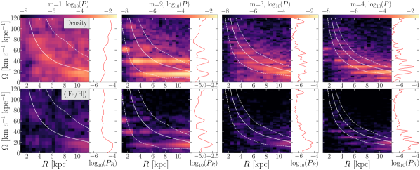
Figure 4: Power spectra (spectrograms) for density (top) and $\left<{\mbox{$\rm[Fe/H]$}}\right>$ (bottom) waves of different multiplicities (columns) at $t=12-13\mbox{$\>{\rm Gyr}$}$. The white solid lines show the rotation curve, $\Omega(R)$, evaluated at the central time of the interval using an interpolated potential. White dashed lines indicate $\Omega\pm\kappa/m$. To the right of each spectrogram we show the radius-integrated power. The colour scale limits are the same for each wave type over all multiplicities and models. The pattern speeds of $m>1$ density and $\left<{\mbox{$\rm[Fe/H]$}}\right>$ waves match each other.

We adopt a similar analysis for the $\left<{\mbox{$\rm[Fe/H]$}}\right>$ pattern speeds, replacing $c_{m}(R_{i},t_{k})$ by $\gamma_{m}(R_{i},t_{k})$. The spectral analysis of the density (i.e. the measurement of the pattern speeds of the bar and spirals) has already been presented by Khachaturyants et al. (2022a) (see their figures 6 and 7). They found that the density Fourier expansion is dominated by $m=2$, with $m=1$ significantly weaker. In Fig. 4 we plot spectrograms of the density (top row) and $\left<{\mbox{$\rm[Fe/H]$}}\right>$ (bottom row) distributions for the time interval $t=12-13\mbox{$\>{\rm Gyr}$}$, for $m=1$ to $m=4$. Each block contains a spectrogram (left) and the radially integrated total power, $P_{R}(\Omega)$ (right) of a given wave. For $m\geq 2$, the spectrograms and total power spectra of the density and $\left<{\mbox{$\rm[Fe/H]$}}\right>$ waves are in good agreement with each other, with the strongest power in $m=2$ (note the different scales of $P_{R}$ for different $m$ in Fig. 4). We therefore restrict our attention to $m=2$ from here on.

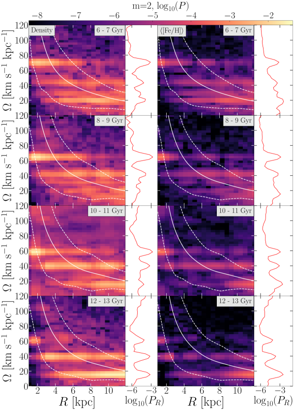
Figure 5: Similar to Fig. 4, but for the power spectra of density (left) and $\left<{\mbox{$\rm[Fe/H]$}}\right>$ (right) $m=2$ waves at the different time intervals (rows) indicated at the top right of each panel.

Fig. 5 therefore shows spectrograms of $m=2$ for the density (left column) and $\left<{\mbox{$\rm[Fe/H]$}}\right>$ (right column) at different times in the evolution of the model. A clear correspondence between the pattern speeds in the density and in $\left<{\mbox{$\rm[Fe/H]$}}\right>$ is evident at each time. When a peak in the power is present in the density we generally find a corresponding peak for $\left<{\mbox{$\rm[Fe/H]$}}\right>$. At the earlier times the disc hosts a larger number of pattern speeds; the number declines to about 3 pattern speeds at later times. The growth and slowdown of the bar from $6\mbox{$\>{\rm Gyr}$}$ to $\sim 9\mbox{$\>{\rm Gyr}$}$ and its subsequent weakening by $12\mbox{$\>{\rm Gyr}$}$ are also evident in the strong feature at $60-80\mbox{$\>{\rm km\,s^{-1}\,kpc^{-1}}$}$.

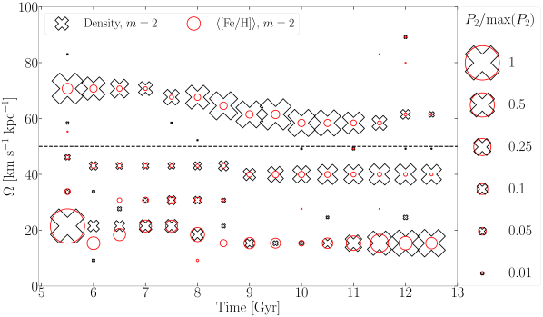
Figure 6: The most prominent pattern speeds for the $m=2$ density (black crosses) and $\left<{\mbox{$\rm[Fe/H]$}}\right>$ (red circles) waves. The marker size is indicative of the radius-integrated power at a given pattern speed. The peaks are scaled by the highest peak in the particular type of wave (density or $\left<{\mbox{$\rm[Fe/H]$}}\right>$) over all baselines, $P_{2}/\rm{max}(P_{2})$ with the legend showing the relationship between the marker size and $P_{2}/\rm{max}(P_{2})$. Only pattern speeds with $P_{2}/\rm{max}(P_{2})\geq 0.01$ are shown. We observe a correspondence between the $m=2$ density and $\left<{\mbox{$\rm[Fe/H]$}}\right>$ perturbations: for the most part, the pattern speeds of the two match, except for the weakest patterns. The horizontal dashed line shows $\Omega=49\mbox{$\>{\rm km\,s^{-1}\,kpc^{-1}}$}$; the region above this frequency is dominated by the bar. Each marker is shown at the mid-point of the corresponding Fourier time series; since these are $1\mbox{$\>{\rm Gyr}$}$ long, consecutive points are correlated (data points in the second half of each time series are the first half of the next time series).

The temporal evolution of the $m=2$ pattern speeds in the density (black crosses) and $\left<{\mbox{$\rm[Fe/H]$}}\right>$ (red circles) can be seen in Fig. 6. The most prominent density perturbations, including the bar, but also the slower spirals, have pattern speeds that are well matched by pattern speeds in the metallicity. Conversely, in almost all cases, the pattern speeds identified in $\left<{\mbox{$\rm[Fe/H]$}}\right>$ are matched by pattern speeds in the density. The size of the markers represents the power normalised by the maximum power value each pattern reaches over the entire time interval of this analysis, i.e. $5-13~{}\mbox{$\>{\rm Gyr}$}$. The density and $\left<{\mbox{$\rm[Fe/H]$}}\right>$ patterns fail to match only for the weakest waves (smallest markers).

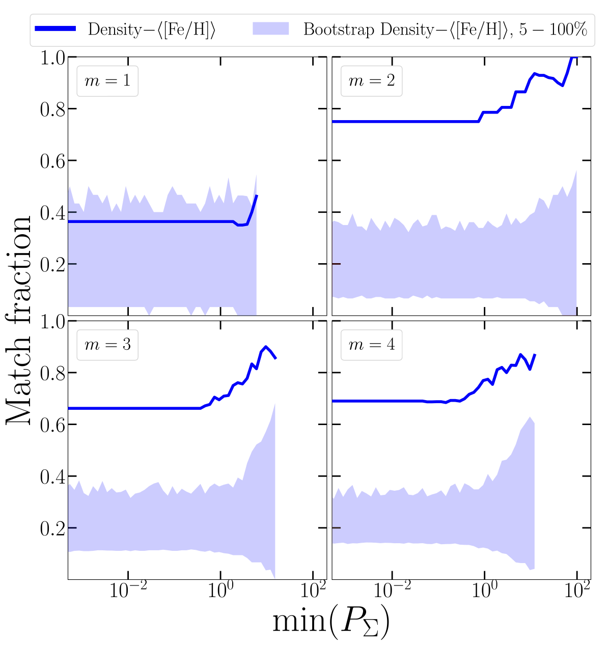
Figure 7: Match fraction between the density and $\left<{\mbox{$\rm[Fe/H]$}}\right>$ waves, given by Eqn. 7, versus the minimum power of the density waves, $\min(P_{\Sigma})$. The shaded region indicates the $5\%$ to $100\%$ distribution of the match fractions resulting from a bootstrap resampling of random pattern speeds of $\left<{\mbox{$\rm[Fe/H]$}}\right>$ waves. All random bootstrap samples have match fraction lower than in the simulation for $m>1$, implying the matches are not random. For this analysis we only consider pattern speeds $\Omega\leq 49\mbox{$\>{\rm km\,s^{-1}\,kpc^{-1}}$}$ (the dashed horizontal line in Fig. 6), to exclude the bar. We do not show $\min(P_{\Sigma})$ with less than 10 identified pattern speeds across all times. For $m>1$, we note an increase in match fraction with increasing $\min(P_{\Sigma})$ that substantially exceeds the random bootstrap-sampled match fractions.

Khachaturyants et al. (2022b) showed that there is a strong connection between spirals and breathing waves by showing that the pattern speeds of strong breathing waves are always matched by pattern speeds of density waves, and vice versa. They argued therefore that the breathing motions must be part of the nature of spirals. As in Khachaturyants et al. (2022b), we quantify the significance of the match between the density and the $\left<{\mbox{$\rm[Fe/H]$}}\right>$ waves in Fig. 7 by showing the fraction of identified density pattern speeds that are matched by pattern speeds in $\left<{\mbox{$\rm[Fe/H]$}}\right>$ (solid lines). The match fraction is defined as the ratio of the number of density pattern speeds with metallicity matches to the total number of density pattern speeds, i.e.:

$$f=\frac{N(\Omega_{\rm{dens+met}})}{N(\Omega_{\rm{dens}})},$$ (7)

where $N(\Omega_{\rm{dens}})$ ($N(\Omega_{\rm{dens+met}})$) is the number of density pattern speeds above the threshold (the number of density pattern speeds above the threshold that are matched by a metallicity pattern speed) for the full time interval $5-13~{}\mbox{$\>{\rm Gyr}$}$ (not just a single time). In order to avoid including the bar, we consider only $\Omega_{p}<49\mbox{$\>{\rm km\,s^{-1}\,kpc^{-1}}$}$ for each multiplicity and baseline. This fraction is shown for different minimum power thresholds of the density pattern speeds, $\min(P_{\Sigma})$. The different panels show the matches for different wave multiplicities. Better matches between the density and $\left<{\mbox{$\rm[Fe/H]$}}\right>$ waves occur for $m>1$. We check if these match fractions are compatible with random matches via a bootstrap algorithm where we select 2500 iterations of random pattern speeds, with a time distribution exactly matching those of the $\left<{\mbox{$\rm[Fe/H]$}}\right>$ waves, and compute the match fraction with the density pattern speeds as before. Fig. 7 presents the $5-100\%$ probability intervals (shaded regions) of the match fraction for these random samples. Only in the case of the $m=1$ waves are the match fractions compatible with the random matches, while $m>1$ match fractions are clearly higher than random at all $\min(P_{\Sigma})$. Since we have binned the $\left<{\mbox{$\rm[Fe/H]$}}\right>$ field, and computed the Fourier time series only of the binned values, the metallicity time series is not contaminated by the density. As a result, the pattern speeds of the two would be independent of each other if the two were unrelated. The high match probability we find therefore indicates that the $\left<{\mbox{$\rm[Fe/H]$}}\right>$ variations are due to the spirals. Thus we conclude that the $\left<{\mbox{$\rm[Fe/H]$}}\right>$ waves are driven by density waves and, in the disc, we must identify them with spirals. It remains to be understood how spirals cause the $\left<{\mbox{$\rm[Fe/H]$}}\right>$ variations.

5 Dissection by age

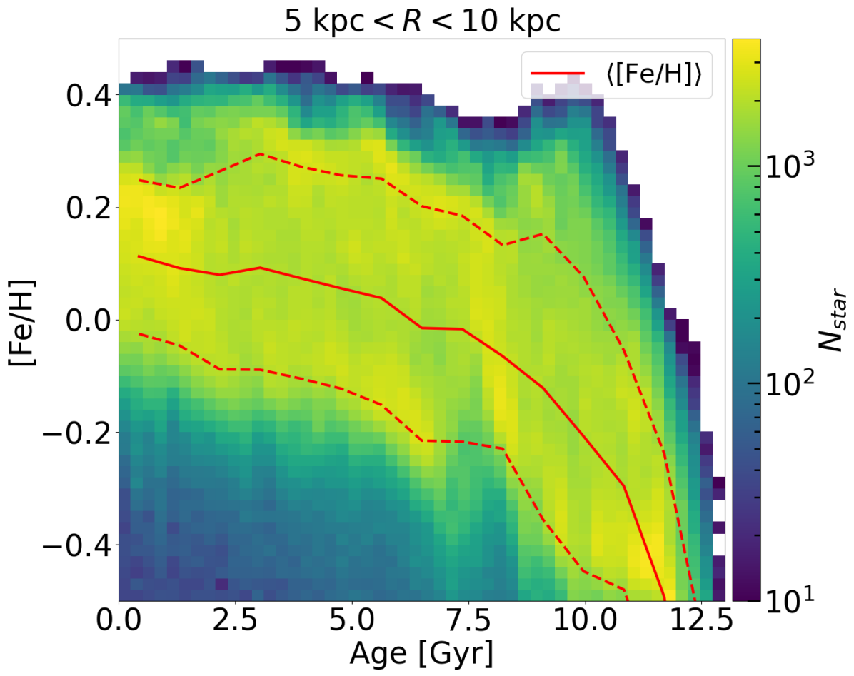
Figure 8: The age-metallicity relation for star particles at $5\leq R/\mbox{$\>{\rm kpc}$}\leq 10$ at $13~{}\mbox{$\>{\rm Gyr}$}$. The solid red line shows $\left<{\mbox{$\rm[Fe/H]$}}\right>$ while the red dashed lines show the $16\%$ and $84\%$ distributions.

Having shown that the $\left<{\mbox{$\rm[Fe/H]$}}\right>$ variations are part of the spirals, and do not result from recent star formation, we next explore the physical mechanism of the $\left<{\mbox{$\rm[Fe/H]$}}\right>$ variations.

First we consider whether $\left<{\mbox{$\rm[Fe/H]$}}\right>$ variations reflect variations in the mean age. Fig. 8 shows the age-metallicity relation (AMR) of stars between $5\mbox{$\>{\rm kpc}$}$ and $10\mbox{$\>{\rm kpc}$}$. A quite shallow relation is evident for stars younger than $\sim 8\mbox{$\>{\rm Gyr}$}$, getting steeper for older stars. The scatter in $\rm[Fe/H]$ increases with age. We have also checked that the AMR of different subsections of this radial range look reasonably similar. The existence of an AMR implies that, if populations of different age have spirals of different amplitude, then azimuthal variations in $\left<{\mbox{$\rm[Fe/H]$}}\right>$ would arise from the azimuthal variation of the spiral amplitude (e.g. Khoperskov et al., 2018).

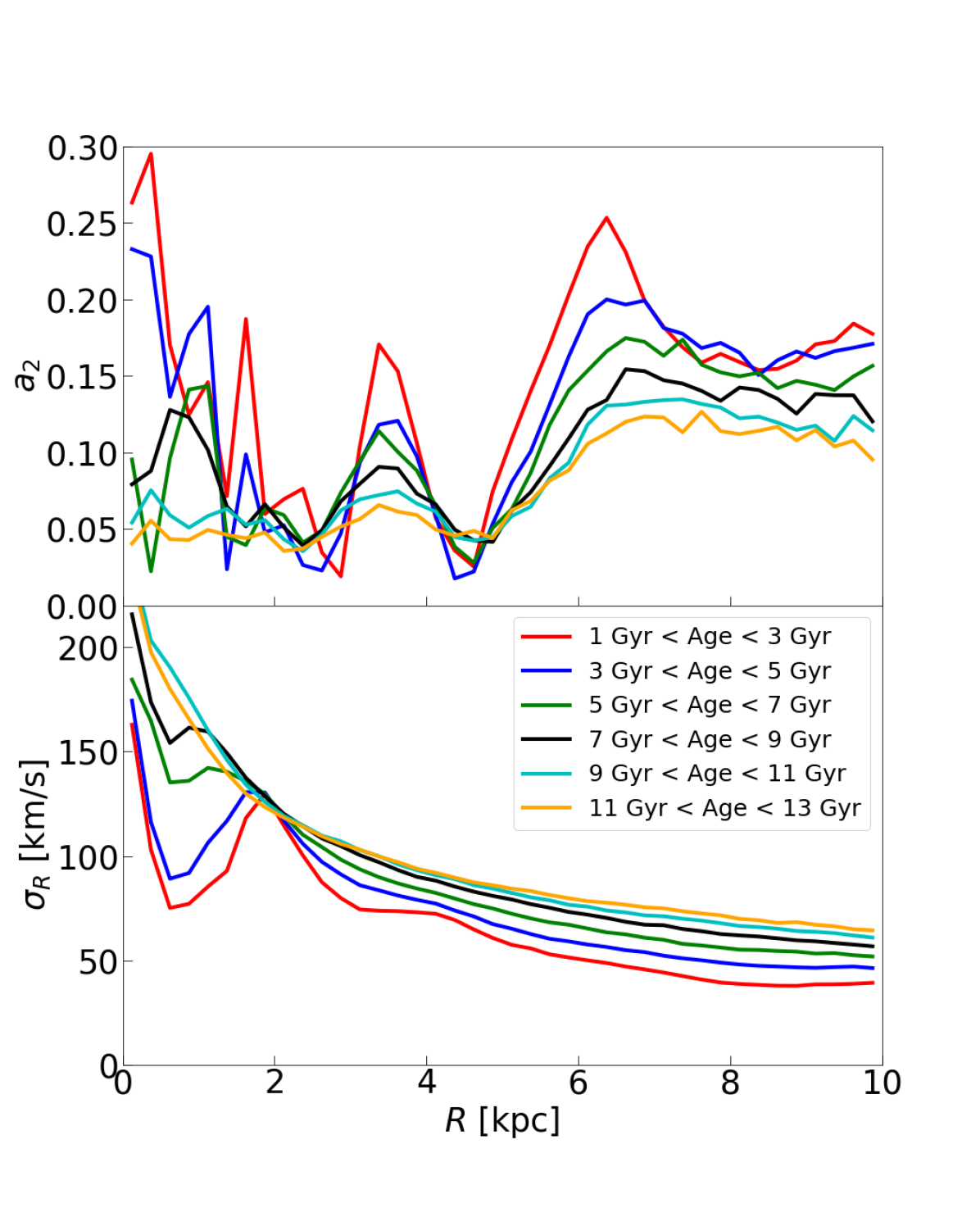
Figure 9: Top: The radial profiles of the amplitude of the $m=2$ density Fourier moments for different age populations, as indicated in the legend. Outside $5\mbox{$\>{\rm kpc}$}$, spiral structure is weaker in old populations than in younger ones. Bottom: The radial velocity dispersion, $\sigma_{R}$, profiles of the same stellar populations. Stars younger than $1\mbox{$\>{\rm Gyr}$}$ are not plotted.

The top panel of Fig. 9 plots the radial profiles of the $m=2$ amplitude of the density; it shows that spirals at $R>5\mbox{$\>{\rm kpc}$}$ are present in all age populations, although they are weaker in older populations, as seen already in Fig. 3 (see also Ghosh et al., 2022). The bottom panel shows that the older populations support weaker spirals because their radial velocity dispersion, $\sigma_{R}$, is higher.

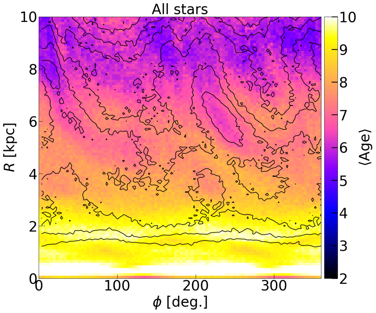
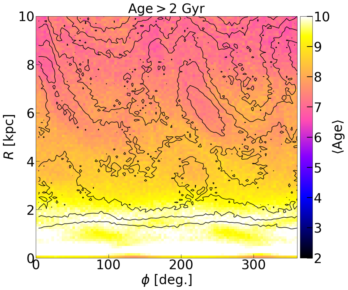
Figure 10: Mean age, $\left<\tau\right>$, in cylindrical coordinates. Top: all stars. Bottom: stars older than $2~{}\mbox{$\>{\rm Gyr}$}$. The contours correspond to the surface density. The disc is rotating in a counter-clockwise sense, i.e. rotation is in the direction of increasing $\phi$. The model is shown at $13~{}\mbox{$\>{\rm Gyr}$}$.

Fig. 10 shows maps of the mean age, $\left<\tau\right>$. The top panel, which includes all stars, shows age variations, which have similar spatial distribution as the metallicity variations of Fig. 1. The bottom panel shows $\left<\tau\right>$ excluding stars younger than $2~{}\mbox{$\>{\rm Gyr}$}$. The variations in $\left<\tau\right>$ retain a similar character to those of the full population, showing again that recent star formation is not the cause of the azimuthal variations. As expected, the spiral ridges are regions of younger stars, which follows because these stars have lower radial velocity dispersions and thus host stronger spirals (Fig. 9).

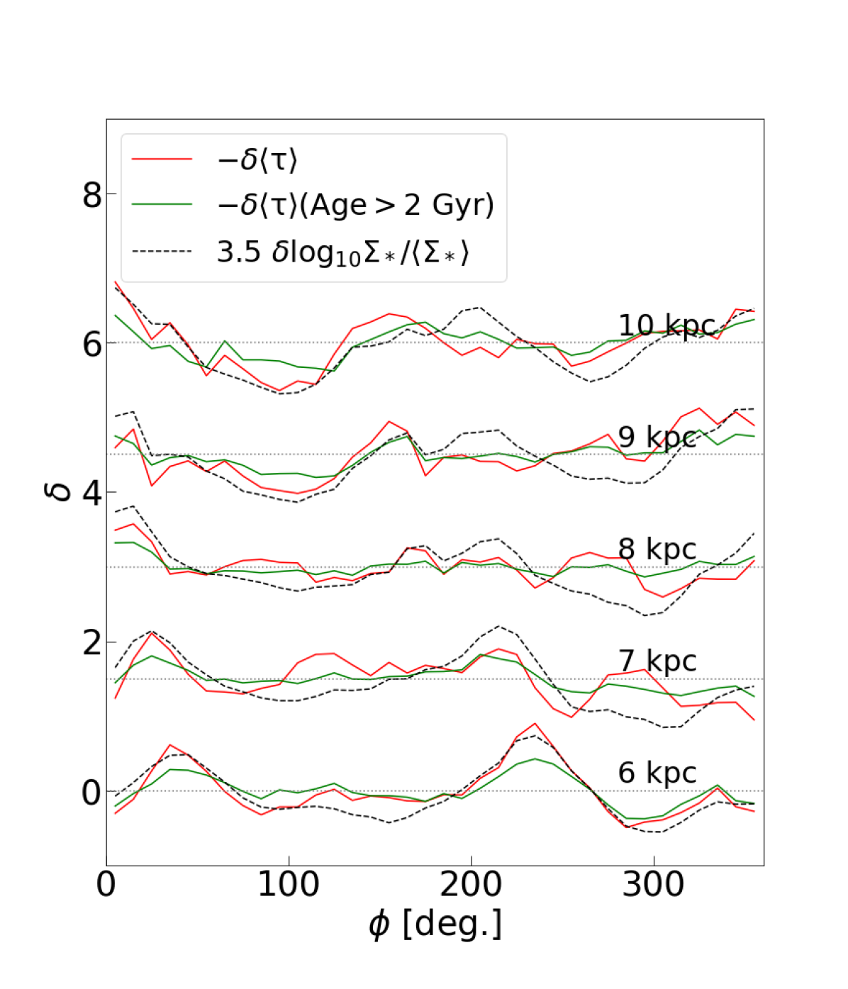
Figure 11: The variation of $\left<\tau\right>$ compared with the density variation at a series of $500~{}\mbox{$\>{\rm pc}$}$-wide annuli centred at $6\mbox{$\>{\rm kpc}$}$ to $10\mbox{$\>{\rm kpc}$}$, as indicated. (We use $-\mbox{$\left<\tau\right>$}$ to permit easier comparison with the density.) The average value at each radius is subtracted from each azimuthal profile and the profiles are then vertically offset by a fixed amount to show the variation. The azimuthal profiles of the density have been scaled by the factor $3.5$ for ease of comparison. The dotted horizontal lines indicate the zero for each radius. The red (green) lines show $\left<\tau\right>$ profiles of all stars (stars older than $2~{}\mbox{$\>{\rm Gyr}$}$).

Fig. 11 compares the azimuthal variation of $\left<\tau\right>$ and the density at different radii. Age variations of order $0.5-1\mbox{$\>{\rm Gyr}$}$ are present at all radii. The green lines in Fig. 11 show the azimuthal profiles of $\left<\tau\right>$ when stars younger than $2\mbox{$\>{\rm Gyr}$}$ are excluded. The azimuthal variations are now weaker, but still evident. Moreover these profiles largely track those of all stars where the deviation from the radial average is significant. Note that the density peaks correspond to locations where the stars are, on average, younger.

While there is a reasonably good correspondence between the variation of the density and mean age, comparison with Fig. 2 shows that $\left<{\mbox{$\rm[Fe/H]$}}\right>$ traces the density variations slightly better than $\left<\tau\right>$ does. This is particularly evident at larger radii. $\left<\tau\right>$ therefore is probably not directly the driver of the $\left<{\mbox{$\rm[Fe/H]$}}\right>$ variations. In any case, the variations in $\left<\tau\right>$ are too small, given the AMR, to be directly responsible for the variations in $\left<{\mbox{$\rm[Fe/H]$}}\right>$.

6 Dependence on the radial action

We have shown above that older populations with larger $\sigma_{R}$ have weaker spirals. The radial motions of individual stars are best quantified by the radial action, $J_{R}$, which is an integral of motion when a system evolves adiabatically. We therefore expect to see strong correlations between the azimuthal variations of $\left<{\mbox{$\rm[Fe/H]$}}\right>$ and those of $\left<{\mbox{$J_{R}$}}\right>$. To test this idea, we compute the actions of the model using the axisymmetric Stäckel fudge of Binney (2012), as implemented in the agama package (Vasiliev, 2019).

6.1 Instantaneous radial actions

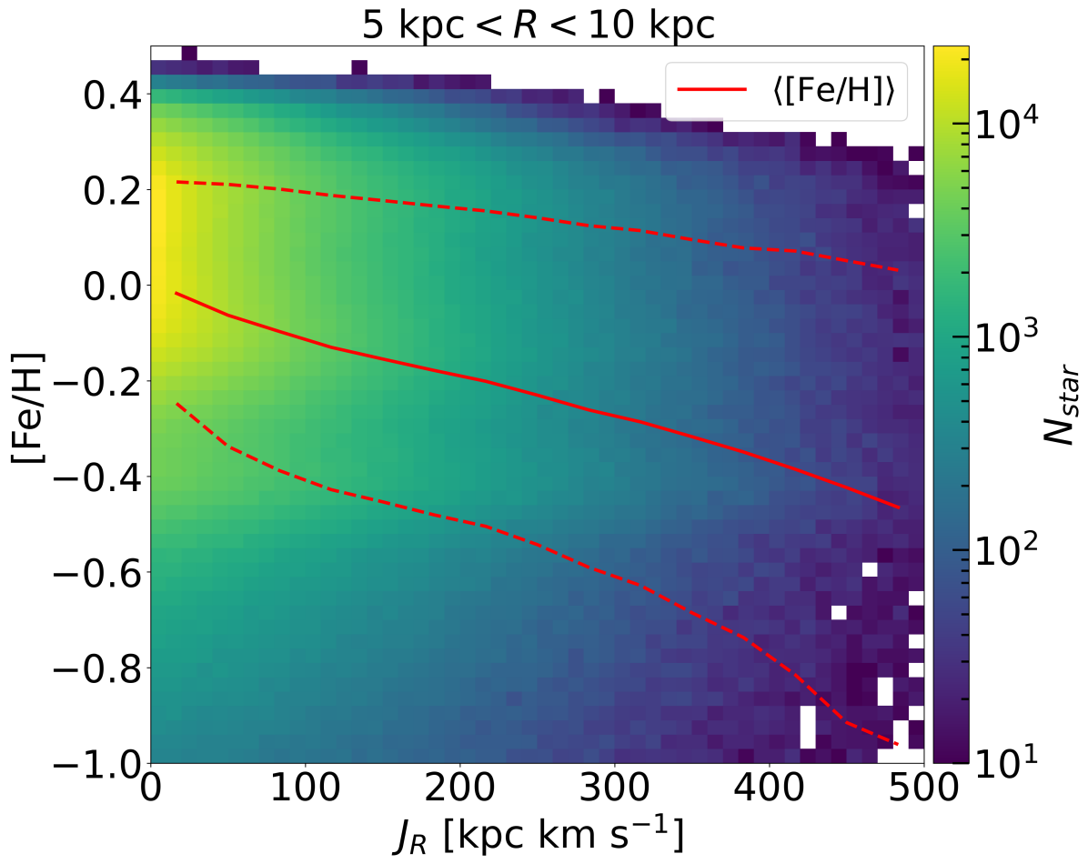
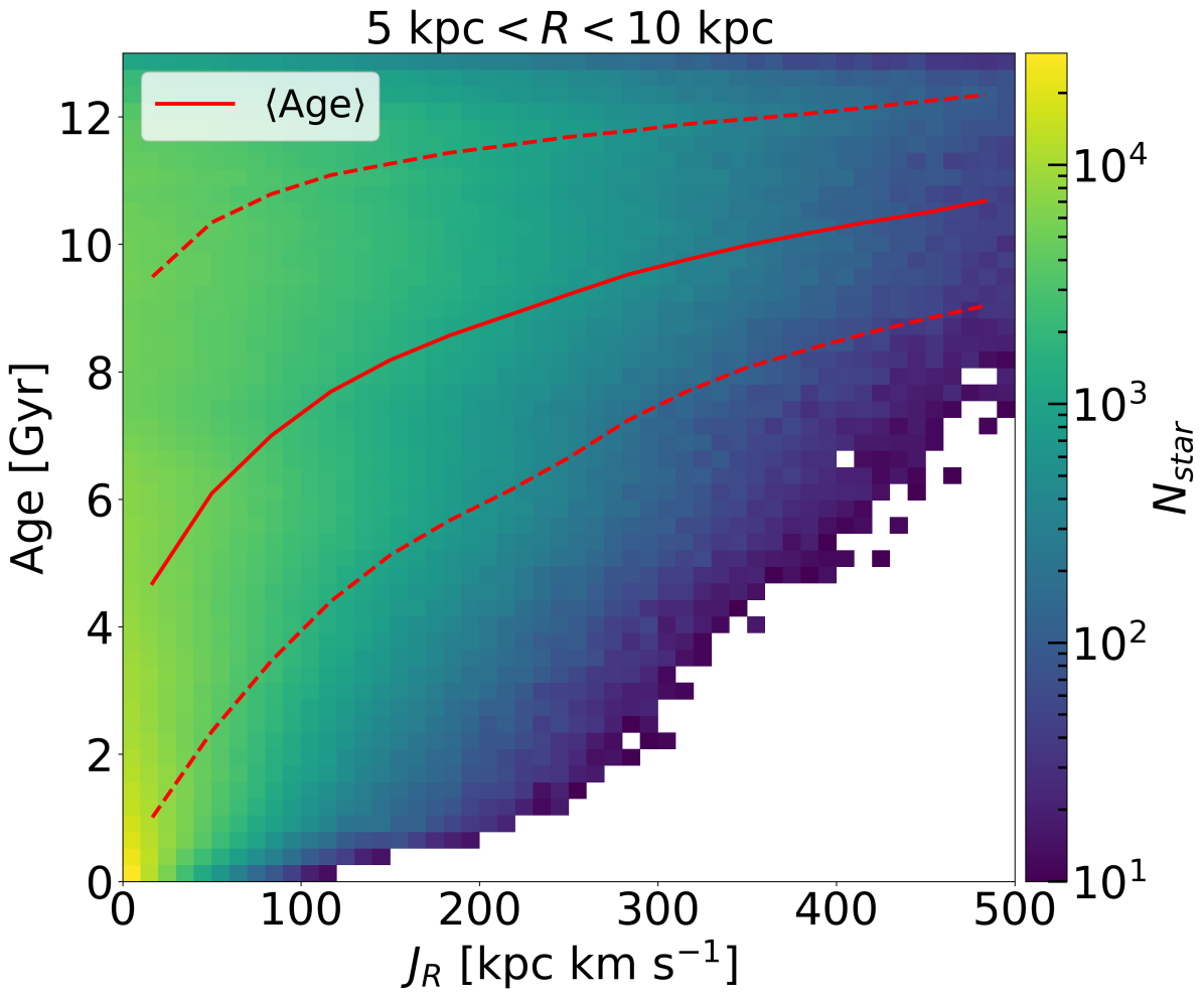
Figure 12: The $J_{R}$-$\rm[Fe/H]$ relation (top) and the $J_{R}$-$\tau$ relation (bottom) for star particles at $5\leq R/\mbox{$\>{\rm kpc}$}\leq 10$ at $13~{}\mbox{$\>{\rm Gyr}$}$. The solid lines show $\left<{\mbox{$\rm[Fe/H]$}}\right>$ (top) and $\left<\tau\right>$ (bottom). In both panels the red dashed curves show the $16\%$ and $84\%$ distributions.

The top panel of Fig. 12 shows the $J_{R}$-$\rm[Fe/H]$ relation. Across the range in $J_{R}$ the mean metallicity varies significantly, and nearly uniformly, although the scatter about the mean is large. The bottom panel shows the $J_{R}$-$\tau$ relation. The average age grows rapidly at low $J_{R}$ and then flattens somewhat. These relations suggest that the driver of the azimuthal variations of stellar populations may be $J_{R}$, which both determines how strong the spiral structure is in a given population, and what the mean metallicity is.

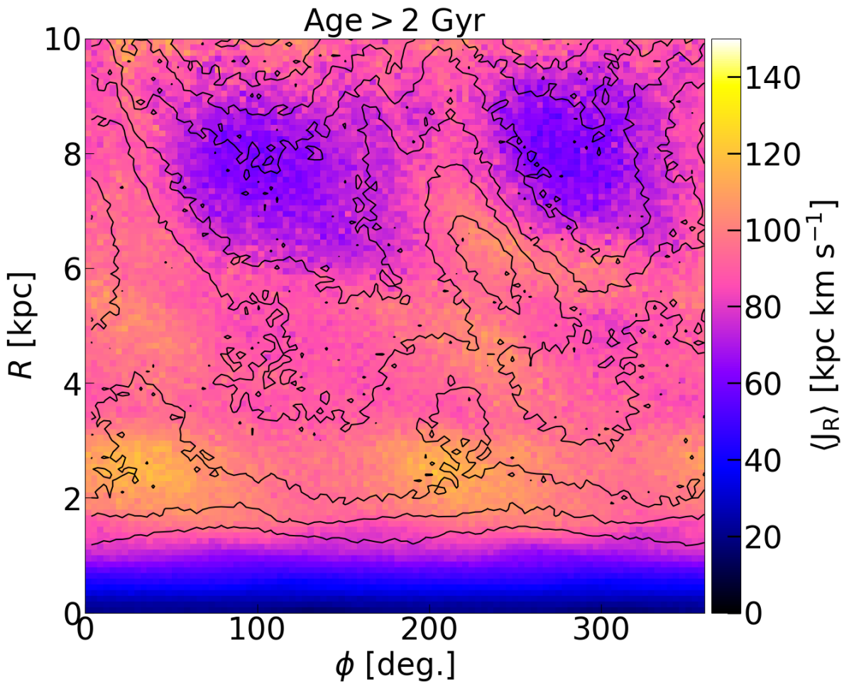
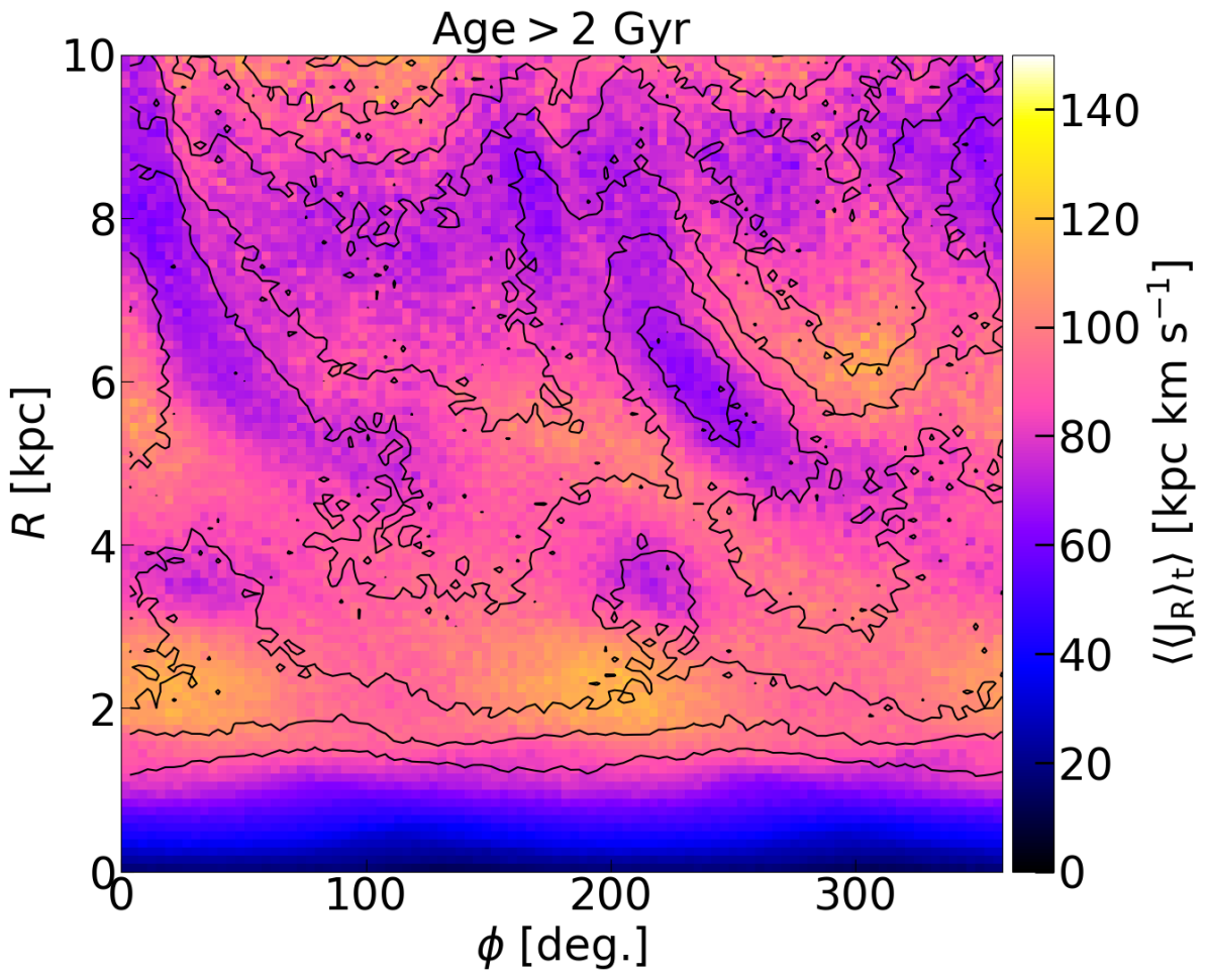
Figure 13: The mean instantaneous radial action, $\left<{\mbox{$J_{R}$}}\right>$, (top) and the mean time-averaged radial action, $\left<{\mbox{$\left<{\mbox{$J_{R}$}}\right>_{t}$}}\right>$, (bottom) in cylindrical coordinates. The contours correspond to the surface density. Only stars older than $2~{}\mbox{$\>{\rm Gyr}$}$ have been considered. The disc is rotating in a counter-clockwise sense, i.e. rotation is in the direction of increasing $\phi$. The model is shown at $13~{}\mbox{$\>{\rm Gyr}$}$.

The top panel of Fig. 13 maps the average radial action, $\left<{\mbox{$J_{R}$}}\right>$, excluding stars younger than $2\mbox{$\>{\rm Gyr}$}$. Significant variations are evident, with $\left<{\mbox{$J_{R}$}}\right>$ maxima near the locations of density peaks. However at some radii (e.g. $6.5~{}\mbox{$\>{\rm kpc}$}$) the location of the $\left<{\mbox{$J_{R}$}}\right>$ peaks are clearly offset from the location of the density peaks. The left panel of Fig. 14, which compares the variations of the density and of $\left<{\mbox{$J_{R}$}}\right>$, also shows that the peaks and troughs are azimuthally offset relative to each other, with the offset varying with radius.

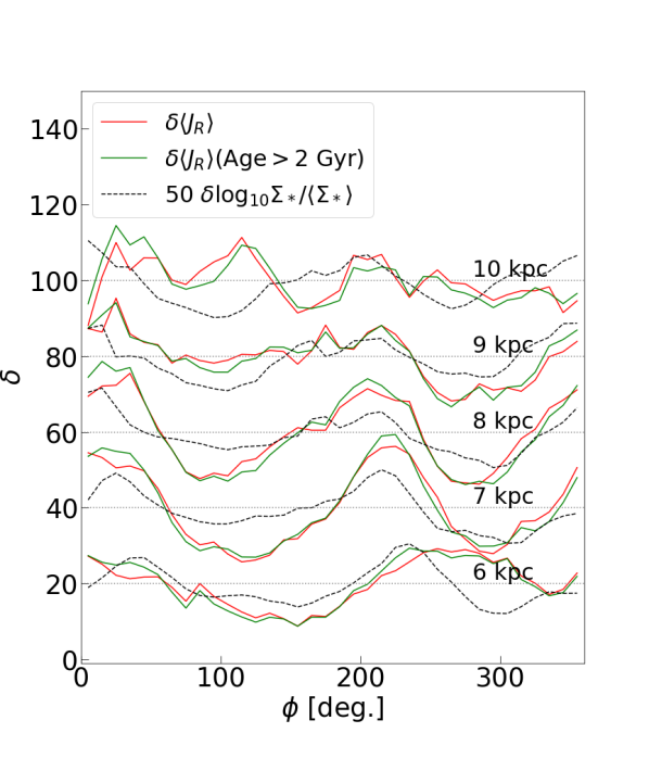
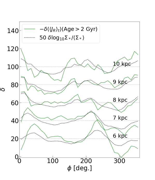
Figure 14: The variation of $\left<{\mbox{$J_{R}$}}\right>$ (left) and $-\mbox{$\left<{\mbox{$\left<{\mbox{$J_{R}$}}\right>_{t}$}}\right>$}$ (note the sign difference) compared with the density variation at a series of $500~{}\mbox{$\>{\rm pc}$}$-wide annuli centred at $6\mbox{$\>{\rm kpc}$}$ to $10\mbox{$\>{\rm kpc}$}$, as indicated. The average value at each radius is subtracted from each azimuthal profile and the profiles are then vertically offset by a fixed amount to show the variation. The azimuthal profiles of the density have been scaled by the factor $50$ for ease of comparison. The dotted horizontal lines indicate the zero for each radius. The red lines show $\left<{\mbox{$J_{R}$}}\right>$ profiles of all stars (left), while the green lines show stars older than $2~{}\mbox{$\>{\rm Gyr}$}$ only (both panels).

Figs. 13 (top) and 14 (left) are puzzling because they imply that, broadly speaking, the spiral density peaks are better traced by stars with large $J_{R}$, which should be older, and therefore represent $\rm[Fe/H]$-poor stars. However we have seen that the $\left<{\mbox{$\rm[Fe/H]$}}\right>$-peaks are located at the density peaks. Moreover, in Fig. 9 we showed that older populations are hotter and host weaker spirals, contradicting the behaviour seen in $J_{R}$.

We resolve this difficulty in the next section by showing that the inherent assumption of axisymmetry in computing $J_{R}$ gives rise to correlated errors.

6.2 Time-averaged radial actions

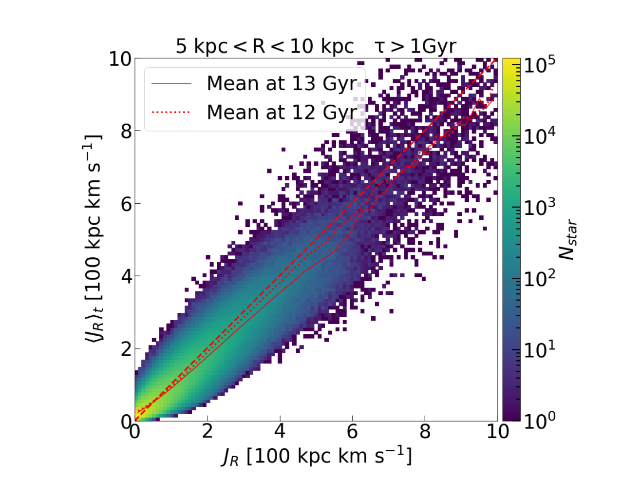
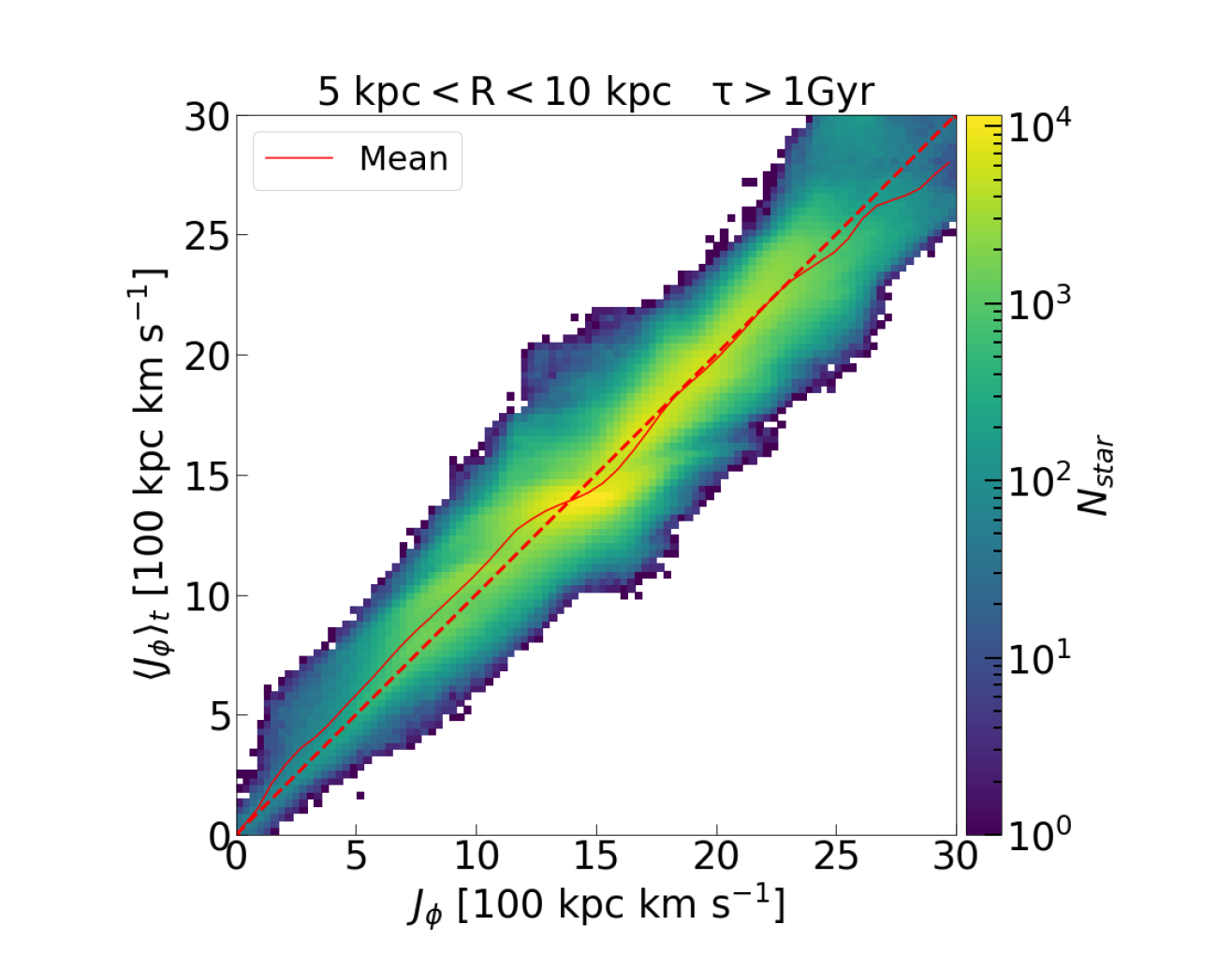
Figure 15: Comparison of $\left<{\mbox{$J_{R}$}}\right>_{t}$ and $J_{R}$ (top) and $\left<{\mbox{$J_{\phi}$}}\right>_{t}$ and $J_{\phi}$ (bottom) for stars which are at $5\leq R/\mbox{$\>{\rm kpc}$}\leq 10$ at $13\mbox{$\>{\rm Gyr}$}$. The dashed lines show the diagonal, $\mbox{$J_{x}$}=\mbox{$\left<{\mbox{$J_{x}$}}\right>_{t}$}$ while the solid lines show the mean relation. The radial action shows the effect of modest heating while the angular momentum shows the effect of migration via resonances. Stars younger than $1\mbox{$\>{\rm Gyr}$}$ are not included. In the top panel the dotted line shows the mean $J_{R}$ if we instead use $J_{R}$ at $12\mbox{$\>{\rm Gyr}$}$ on the horizontal axis.

Because agama assumes axisymmetry when computing actions, subtle but spurious correlations between the azimuthal phase of a star with respect to a spiral and its computed $J_{R}$ may arise. In order to mitigate, somewhat, such effects, we also compute the time average of $J_{R}$, which we denote $\left<{\mbox{$J_{R}$}}\right>_{t}$. We carry out these time averages over a $1\mbox{$\>{\rm Gyr}$}$ time interval. This is long enough for stars to have drifted across spirals several times. For those stars trapped at the corotation resonance, $1\mbox{$\>{\rm Gyr}$}$ is long compared to the lifetimes of transient spirals (see Roškar et al., 2012), so that they will not have been trapped throughout this time. As can be seen in Fig. 4, the inner Lindblad resonances (ILRs) of the spirals are inside $R=5\mbox{$\>{\rm kpc}$}$, so, in the region we are interested in, the heating will generally be due to the outer Lindblad resonances (OLR), which is generally milder (Sellwood & Binney, 2002). We compute the actions at $21$ snapshots, between $12~{}\mbox{$\>{\rm Gyr}$}$ and $13~{}\mbox{$\>{\rm Gyr}$}$, inclusive, and average $J_{R}$ to obtain $\left<{\mbox{$J_{R}$}}\right>_{t}$.

We compare the time-averaged radial action to the instantaneous one (at $13\mbox{$\>{\rm Gyr}$}$) in the top panel of Fig. 15. The mean of the distribution is slightly offset towards larger $J_{R}$; this is probably the effect of stellar orbit heating during this time interval. We can indeed see, in the bottom panel of Fig. 9, that stellar populations are slowly heating. The distribution is broadened, extending to $\mbox{$\left<{\mbox{$J_{R}$}}\right>_{t}$}>\mbox{$J_{R}$}$, suggesting that the instantaneous action is varying significantly over the $1\mbox{$\>{\rm Gyr}$}$ time interval. The most likely cause of this variation is that the assumption of axisymmetry is introducing errors in the measurement.

The distribution in the top panel of Fig. 15 appears featureless. In contrast, the comparable plot for $J_{\phi}$-$\left<{\mbox{$J_{\phi}$}}\right>_{t}$ (bottom panel) shows clear features over the same time interval. These features are likely produced by the radial migration driven by transient spirals (Sellwood & Binney, 2002).

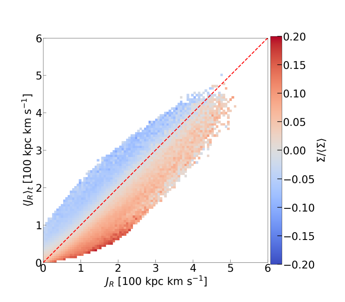
Figure 16: The density variation of individual stars at $t=13\mbox{$\>{\rm Gyr}$}$ in ($J_{R}$,$\left<{\mbox{$J_{R}$}}\right>_{t}$)-space. The deviation of $J_{R}$ from the diagonal line is highly correlated with the over-density. Only bins with more than 20 particles are shown.

To confirm the hypothesis that the instantaneous value of $J_{R}$ is being perturbed by the spirals, we measure the overdensity of individual particles, $\Sigma/\left<\Sigma\right>$, where $\left<\Sigma\right>$ is the azimuthally averaged density. We measure the local density by constructing a KD tree of the star particle distribution based on the Euclidean 2D mid-plane distances using the scipy.spatial.KDTree package. For each particle we measure the distance to the nearest 32 particles and compute the density over these particles, and then compute the ratio of the particle’s density and the azimuthal average. We plot the $\left<{\mbox{$J_{R}$}}\right>_{t}$-$J_{R}$ distribution coloured by this density excess in Fig. 16. The deviation of the instantaneous $J_{R}$ from the diagonal is very well correlated with the excess density, indicating that $J_{R}$ has correlated errors.

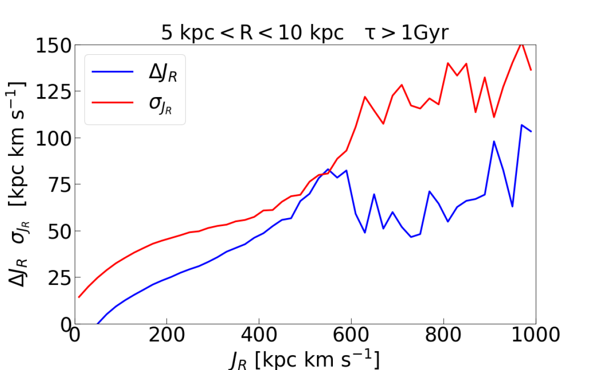
Figure 17: The heating, $\Delta\mbox{$J_{R}$}=\mbox{$\left<{\mbox{$J_{R}$}-\mbox{$\left<{\mbox{$J_{R}$}}\right>_{t}$}}\right>$}$ (blue), and the instantaneous radial action measurement uncertainty, $\sigma_{\mbox{$J_{R}$}}$, computed as the standard deviation of $(\mbox{$J_{R}$}-\mbox{$\left<{\mbox{$J_{R}$}}\right>_{t}$})$ (red). Only stars older than $1\mbox{$\>{\rm Gyr}$}$ in the disc are considered. See the text for why $\Delta\mbox{$J_{R}$}$ over-estimates the heating.

In order to compare the measurement uncertainty with the heating rate, we first bin particles by $J_{R}$ at $13\mbox{$\>{\rm Gyr}$}$. For each bin, we estimate the uncertainty in the measurement of $J_{R}$ as the the standard deviation in $\left<{\mbox{$J_{R}$}}\right>_{t}$, which we term $\sigma_{\mbox{$J_{R}$}}$. We estimate the heating rate as the difference between $J_{R}$ and the average $\left<{\mbox{$J_{R}$}}\right>_{t}$ in each bin, i.e. $\Delta\mbox{$J_{R}$}=\mbox{$\left<{\mbox{$J_{R}$}-\mbox{$\left<{\mbox{$J_{R}$}}\right>_{t}$}}\right>$}$. Fig. 17 shows our measurements of the heating and $J_{R}$ measurement uncertainty. Over this $1\mbox{$\>{\rm Gyr}$}$ time interval, the heating is smaller than the measurement uncertainty. We interpret this as indicating that the uncertainties in measuring the instantaneous $J_{R}$ based on the assumption of axisymmetry are larger than the radial heating. In reality we have over-estimated the heating, since this is based on the assumption that all the difference between $\left<{\mbox{$J_{R}$}}\right>$ and $\left<{\mbox{$\left<{\mbox{$J_{R}$}}\right>_{t}$}}\right>$, corresponding to the difference between the $1:1$ (dashed) line and the mean $J_{R}$ (solid) line in the top panel of Fig. 15, is due entirely to heating. However, the dotted line in the same panel shows the relation between the same $\left<{\mbox{$J_{R}$}}\right>_{t}$ and $J_{R}$ computed at $12\mbox{$\>{\rm Gyr}$}$, and this line is also below the diagonal. The offset between the diagonal and the solid line, therefore, is partly due to an asymmetric distribution, which means that we have over-estimated the heating rate.

The bottom panel of Fig. 13 maps $\left<{\mbox{$\left<{\mbox{$J_{R}$}}\right>_{t}$}}\right>$ in cylindrical coordinates. The spiral arms are very well delineated by $\left<{\mbox{$\left<{\mbox{$J_{R}$}}\right>_{t}$}}\right>$, much better than by $\left<{\mbox{$J_{R}$}}\right>$ (top panel). The differences between the two maps are quite striking with the peak densities being associated with minima in $\left<{\mbox{$\left<{\mbox{$J_{R}$}}\right>_{t}$}}\right>$ but closer to maxima in $\left<{\mbox{$J_{R}$}}\right>$. That low $\left<{\mbox{$J_{R}$}}\right>_{t}$ should track the spirals is natural since radially cool stars support the spiral structure better. At the same time, the larger radial perturbations these stars experience means that when the actions are computed they will appear to be radially hotter, leading to apparently larger $J_{R}$.

The right panel of Fig. 14 plots the azimuthal variations of $\left<{\mbox{$\left<{\mbox{$J_{R}$}}\right>_{t}$}}\right>$ and compares them with those of the density. Compared with $\left<{\mbox{$J_{R}$}}\right>$ in the left panel, a number of important differences are evident. First we confirm that, while the variations in $\left<{\mbox{$J_{R}$}}\right>$ somewhat correlate with the density variations, those in $\left<{\mbox{$\left<{\mbox{$J_{R}$}}\right>_{t}$}}\right>$ anti-correlate with the density variations, as expected. Furthermore, while the correlation with $\left<{\mbox{$J_{R}$}}\right>$ is relatively poor, that with $\left<{\mbox{$\left<{\mbox{$J_{R}$}}\right>_{t}$}}\right>$ is quite strong. Combined with the $J_{R}$-$\rm[Fe/H]$ relation of Fig. 12 this is able to explain the strong correlation between the density and $\left<{\mbox{$\rm[Fe/H]$}}\right>$ variations.

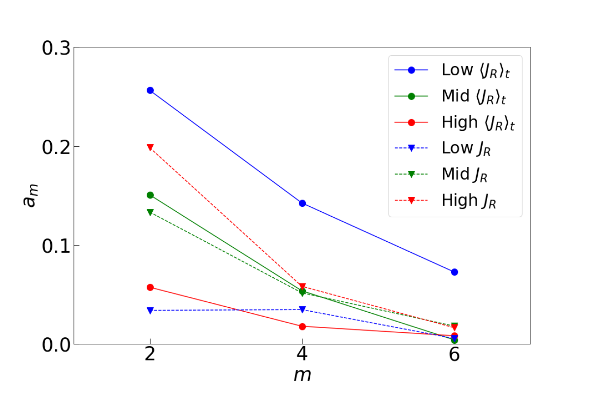
Figure 18: The $m=2$, $4$ and $6$ Fourier amplitudes of the density distribution at $5.5<R/\mbox{$\>{\rm kpc}$}<6.5$ separated into equal-sized low, medium and high populations of $\left<{\mbox{$J_{R}$}}\right>_{t}$ (solid lines) and $J_{R}$ (dashed lines).

Fig. 18 shows the amplitudes of the Fourier amplitudes for $m=2,~{}4$ and $6$, for the stars at $R=6\mbox{$\>{\rm kpc}$}$ (where the spirals are strong) separated into 3 roughly equal-sized populations of low, medium and high $J_{R}$ and $\left<{\mbox{$J_{R}$}}\right>_{t}$. The low $\left<{\mbox{$J_{R}$}}\right>_{t}$ population has the strongest amplitudes, including at $m=6$, indicating that this population is able to support sharp features in the spiral structure. The mid and high $\left<{\mbox{$J_{R}$}}\right>_{t}$ have progressively weaker amplitudes. Instead, in $J_{R}$, the strongest amplitudes are in the high-$J_{R}$ population, although these amplitudes are smaller than the ones in the low-$\left<{\mbox{$J_{R}$}}\right>_{t}$ population. The amplitudes decrease as $J_{R}$ decreases, the opposite of what is expected. Moreover, the $m=6$ amplitude is nearly zero for all $J_{R}$ populations, indicating that sharp features in physical space cannot be represented by $J_{R}$ populations. Clearly $J_{R}$ does a poorer job of tracing the spiral structure than does $\left<{\mbox{$J_{R}$}}\right>_{t}$.

6.3 Correlations

We compute the correlations between the variations in the density, and those of the population properties for stars in the disc region. In other words we quantify the correlations seen in Figures 2, and others like it. From the cylindrical maps (in the radial range $5\leq R/\mbox{$\>{\rm kpc}$}\leq 10$, which covers $N_{\phi}=101$ and $N_{R}=51$ bins, giving $N_{\phi}\times N_{R}=5151$ pixels), we subtract the radial profile of the azimuthal average in each of the quantities of interest (density, $\rm[Fe/H]$, $\rm[O/Fe]$, $\tau$, $J_{R}$, and $\left<{\mbox{$J_{R}$}}\right>_{t}$). We then compute the correlation coefficient between all the pixel values for the density and each of the other variables in turn.

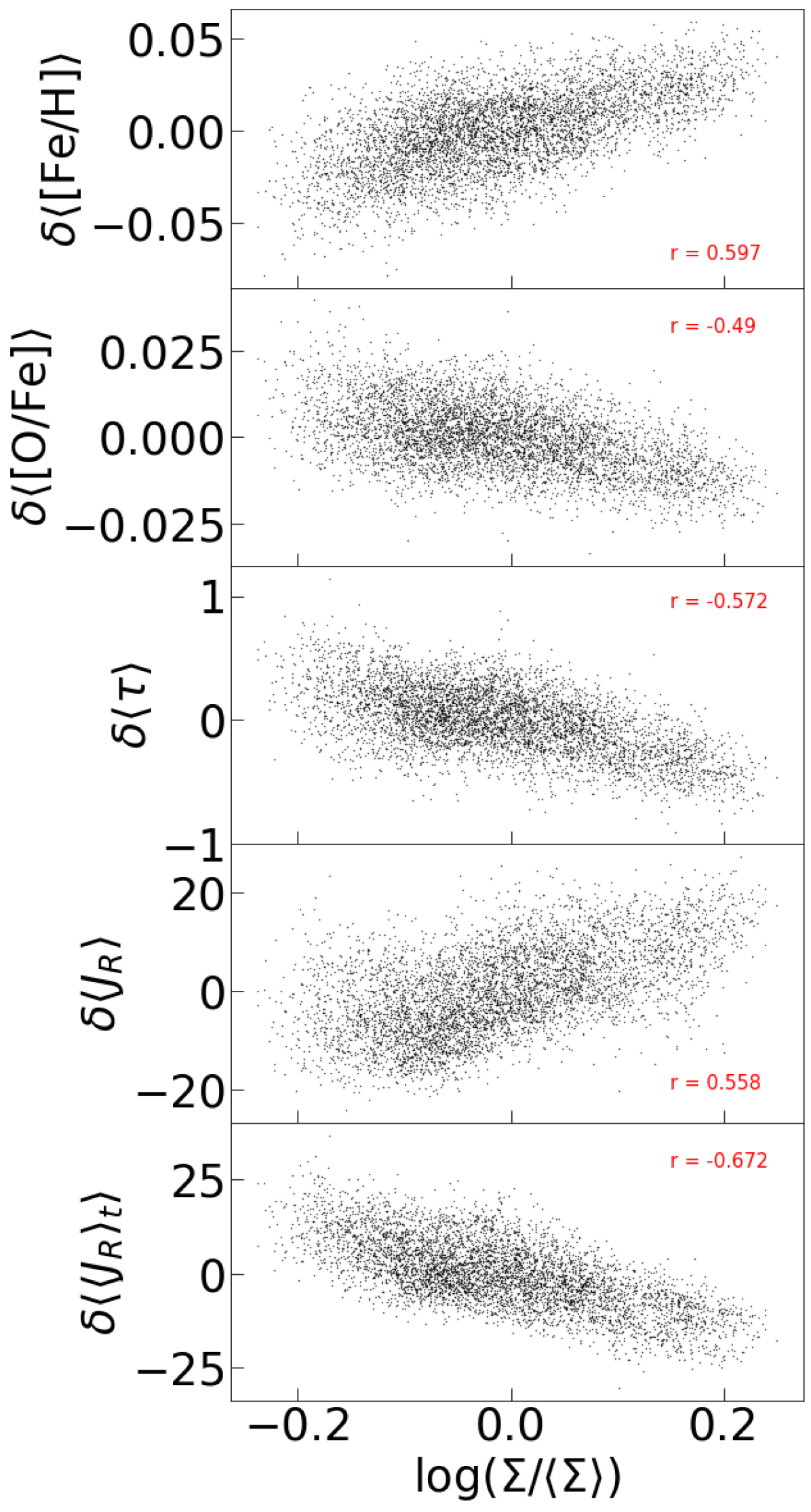
Figure 19: The dependence of azimuthal variations in $\rm[Fe/H]$ (top row), $\rm[O/Fe]$ (second row), $\tau$ (third row), $J_{R}$ (fourth row) and $\left<{\mbox{$J_{R}$}}\right>_{t}$ (bottom row) on the azimuthal variations in density. The Pearson $r$ value of each correlation is indicated in each panel. The strongest correlation is between the density variations and those in the $\left<{\mbox{$J_{R}$}}\right>_{t}$. Note the change in the sign of $r$ for the correlation between the density variations with $\delta\mbox{$\left<{\mbox{$J_{R}$}}\right>$}$ and with $\delta\mbox{$\left<{\mbox{$\left<{\mbox{$J_{R}$}}\right>_{t}$}}\right>$}$. Populations younger than $2~{}\mbox{$\>{\rm Gyr}$}$ are excluded from this plot. The units of $\delta\mbox{$\left<\tau\right>$}$ are $\>{\rm Gyr}$, while the units of $\delta\mbox{$\left<{\mbox{$J_{R}$}}\right>$}$ and $\delta\mbox{$\left<{\mbox{$\left<{\mbox{$J_{R}$}}\right>_{t}$}}\right>$}$ are $\>{\rm kpc\,km\,s^{-1}}$.

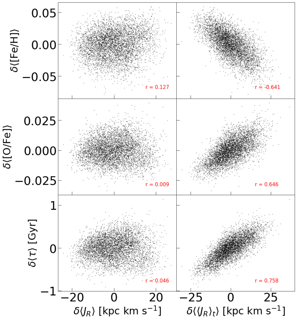
Figure 20: The dependence of variations in stellar population properties, $\delta\mbox{$\left<{\mbox{$\rm[Fe/H]$}}\right>$}$ (top), $\delta\mbox{$\left<{\mbox{$\rm[O/Fe]$}}\right>$}$ (middle) and $\delta\mbox{$\left<\tau\right>$}$ (bottom) on the azimuthal variations of the radial action computed instantaneously, $\delta\mbox{$\left<{\mbox{$J_{R}$}}\right>$}$, (left) and time-averaged, $\delta\mbox{$\left<{\mbox{$\left<{\mbox{$J_{R}$}}\right>_{t}$}}\right>$}$, (right). The Pearson $r$ value of each correlation in indicated in each panel. The population variations are strongly correlated with those of $\left<{\mbox{$J_{R}$}}\right>_{t}$, but very poorly correlated with those of $J_{R}$.

Fig. 19 shows how stellar population properties vary with density variations. The spiral ridges correspond to high $\delta\mbox{$\left<{\mbox{$\rm[Fe/H]$}}\right>$}$, and low $\delta\mbox{$\left<{\mbox{$\rm[O/Fe]$}}\right>$}$ and $\delta\mbox{$\left<\tau\right>$}$. It also shows that the correlation between density variations and $\delta\mbox{$\left<{\mbox{$\left<{\mbox{$J_{R}$}}\right>_{t}$}}\right>$}$ is stronger than that between density variations and $\delta\mbox{$\left<{\mbox{$J_{R}$}}\right>$}$. This latter relation is, in fact, even weaker than the correlation between the density variations and $\delta\mbox{$\left<{\mbox{$\rm[Fe/H]$}}\right>$}$ and $\delta\mbox{$\left<\tau\right>$}$. Even more strikingly, the correlation between the density variations and $\delta\mbox{$\left<{\mbox{$\left<{\mbox{$J_{R}$}}\right>_{t}$}}\right>$}$ is negative (i.e. high density regions have small time-averaged radial action) while the correlation is positive for the instantaneous one. Fig. 20 shows how the variations in the stellar population properties (age, metallicity and $\rm\alpha$-abundance) correlate with the variations in $J_{R}$ and $\left<{\mbox{$J_{R}$}}\right>_{t}$. The stellar population variations are poorly correlated with $\delta\mbox{$\left<{\mbox{$J_{R}$}}\right>$}$ but strongly correlated with $\delta\mbox{$\left<{\mbox{$\left<{\mbox{$J_{R}$}}\right>_{t}$}}\right>$}$. Together, Figs. 19 and 20 demonstrate that the errors associated with the axisymmetric approximation in computing the actions are sufficiently large to mask the actual dependence of the population variations on the radial action.

We have also explored the vertical action, $J_{z}$ and $\left<{\mbox{$J_{z}$}}\right>_{t}$ (defined similar to $\left<{\mbox{$J_{R}$}}\right>_{t}$). We find that $J_{z}$ behaves more similar to $\left<{\mbox{$J_{z}$}}\right>_{t}$, with spiral structure becoming progressively weaker as $J_{z}$ increases. This indicates that the vertical motion is less affected by the spirals than the radial motion, consistent with the idea that in-plane and vertical motions are only weakly coupled.

6.4 Synthesis

In summary, the azimuthal $\left<{\mbox{$\rm[Fe/H]$}}\right>$ variations appear to be the result of the spirals being more strongly supported by stars with low intrinsic $J_{R}$. Such stars are, on average, metal-rich, and relatively young, which means that the locations of the spiral density peaks (troughs) are also where these stars are over (under) represented, giving rise to the mean metallicity peaks (troughs). However recovering this behaviour requires that the radial actions are time averaged to remove correlated errors due to the assumption of axisymmetry in computing them.

7 The view in action space

Resonant trapping leads to action non-conservation, with stars librating around the resonance when viewed in action space. In this section we examine whether the $J_{R}$ variations are due to such librations, rather than errors arising from the axisymmetric approximation.

7.1 Link to migration

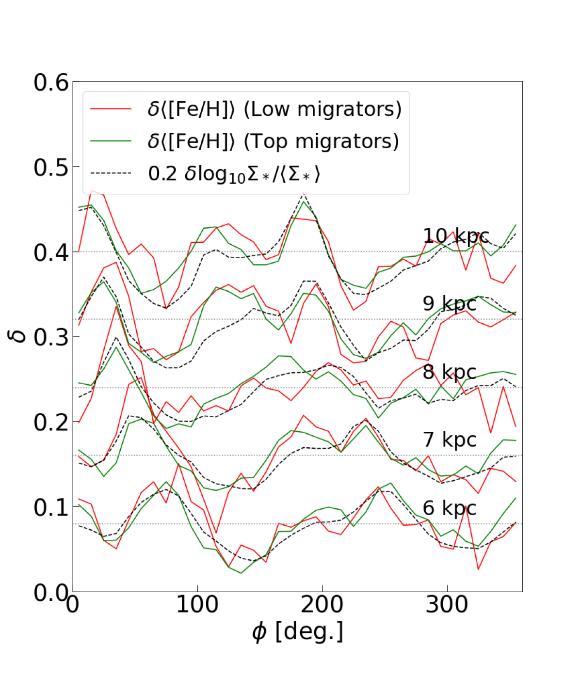
Figure 21: The relation between $\left<{\mbox{$\rm[Fe/H]$}}\right>$ variations and migration over the time interval $12\mbox{$\>{\rm Gyr}$}$ to $13\mbox{$\>{\rm Gyr}$}$. The variation of $\left<{\mbox{$\rm[Fe/H]$}}\right>$ compared with the density variation at a series of 500 pc-wide annuli centred at $6\mbox{$\>{\rm kpc}$}$ to $10\mbox{$\>{\rm kpc}$}$, as indicated. The average values for each radius are subtracted from each azimuthal profile and the profiles are then vertically offset by a fixed amount to show the variation. The azimuthal profiles of the density have been scaled by the factor $0.2$, for ease of comparison. The dotted horizontal lines indicate the zero for each radius. The green (red) lines are for stars that belong to the top (bottom) third of migrators. We show the $12\mbox{$\>{\rm Gyr}$}$ distribution.

Variations in $\left<{\mbox{$\rm[Fe/H]$}}\right>$ have been proposed to be related to migration. In order to test whether migration plays a big role in the $J_{R}$ variations, we separate populations by the amount of migration by computing the change in angular momentum, $\Delta\mbox{$J_{\phi}$}=\left|\mbox{$J_{\phi}$}(12~{}\mbox{$\>{\rm Gyr}$})-\mbox{$J_{\phi}$}(13~{}\mbox{$\>{\rm Gyr}$})\right|$. We split the stars into thirds based on $\Delta\mbox{$J_{\phi}$}$. Fig. 21 shows azimuthal profiles of $\left<{\mbox{$\rm[Fe/H]$}}\right>$ for the high and low migrators (top and bottom thirds of $\Delta\mbox{$J_{\phi}$}$). No significant azimuthal offset between the azimuthal profiles of these two populations are evident. We find no support for the idea that migration dominates the azimuthal variations in $\left<{\mbox{$\rm[Fe/H]$}}\right>$, although it may contribute when metallicity gradients are steep (Grand et al., 2016a; Khoperskov et al., 2018).

7.2 The role of resonances

We now consider the joint time-evolution of $J_{R}$ and $J_{\phi}$, in order to show that the variations in $J_{R}$ we have found are not due to resonances.

Recall that when a resonance is present, stars are either trapped by it, in which case their actions librate back and forth across the resonant action, or they are untrapped, in which case their actions vary periodically while the stars rotate. The variations of $J_{R}$ and $J_{\phi}$ of both trapped and untrapped stars can be related by noting that the Jacobi energy, $E_{J}\equiv E-\mbox{$\Omega_{\rm p}$}\mbox{$J_{\phi}$}$, is a conserved quantity (e.g. Binney & Tremaine, 2008, chapter 3.3.2), where $E$ is a star’s energy and $\Omega_{\rm p}$ the pattern speed of the perturbation, provided that the system is nearly stationary in the rotating frame of the perturber. Thus in the $(\mbox{$J_{\phi}$},\mbox{$J_{R}$})$-plane, resonances cause stars to oscillate tangential to the contours of constant $E_{J}$, even if they are not resonantly trapped.

Furthermore a star is at a planar resonance when $N_{R}\mbox{$\Omega_{R}$}+N_{\phi}(\mbox{$\Omega_{\phi}$}-\mbox{$\Omega_{\rm p}$})=0$, where $N_{R}$ and $N_{\phi}$ are integers and $\Omega_{\phi}$ and $\Omega_{R}$ are a star’s azimuthal and radial frequencies. The principal resonances are the corotation (CR; $N_{R}=0$), and the outer and inner Lindblad resonances (OLR and ILR; $N_{R}=1,~{}N_{\phi}=\pm 2$). The conservation of $E_{J}$ leads to the condition

$$\Delta{\mbox{$J_{R}$}}=\frac{N_{R}}{N_{\phi}}\Delta{\mbox{$J_{\phi}$}}$$ (8)

(e.g. Sellwood & Binney, 2002; Chiba et al., 2021). Therefore, for the ILR, CR and OLR, the directions of oscillation of resonant orbits have slopes $-\frac{1}{2}$, $0$ and $+\frac{1}{2}$, respectively, in the ($J_{\phi}$,$J_{R}$)-plane. We can therefore test whether the variations in $J_{R}$ and $J_{\phi}$ follow these conditions by plotting their evolution in the $(\mbox{$J_{\phi}$},\mbox{$J_{R}$})$-plane.

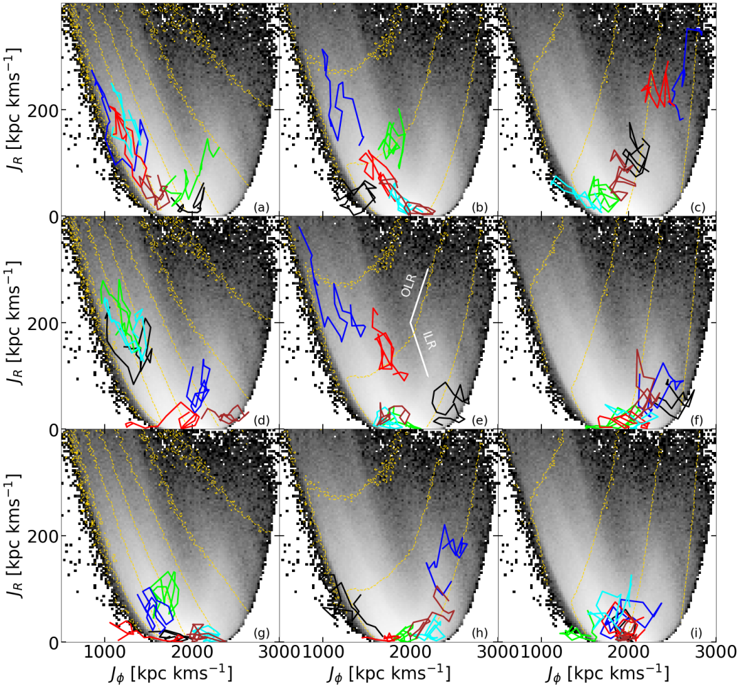
Figure 22: The evolution of a random set of 54 particles, selected as described in the text, in the action space ($J_{\phi}$,$J_{R}$). In each panel we present 6 stars with different colours over a $1\mbox{$\>{\rm Gyr}$}$ time interval plotting every $50\mbox{$\>{\rm Myr}$}$. The plotted particles are ordered by age, with the oldest in the top row ($9.2\leq\mbox{$\tau$}/\mbox{$\>{\rm Gyr}$}\leq 11.7$), the intermediate age ones in the middle row ($4.7\leq\mbox{$\tau$}/\mbox{$\>{\rm Gyr}$}\leq 8.8$) and the youngest in the bottom row ($2.2\leq\mbox{$\tau$}/\mbox{$\>{\rm Gyr}$}\leq 4.2$). The dashed yellow lines show contours of constant $E_{J}$ for $\mbox{$\Omega_{\rm p}$}=15.4~{}\mbox{$\>{\rm km\,s^{-1}\,kpc^{-1}}$}$ (left), $40.0~{}\mbox{$\>{\rm km\,s^{-1}\,kpc^{-1}}$}$ (centre) and $61.5~{}\mbox{$\>{\rm km\,s^{-1}\,kpc^{-1}}$}$ (right). The white lines in panel (e) indicate the libration vectors at the OLR (upper line) and the ILR (lower line). The background shows a log scale representation of the number density of stars.

We carry out this test for a subsample of stars chosen at random. We begin by selecting stars older than $2\mbox{$\>{\rm Gyr}$}$ in the radial region $7\leq R/\mbox{$\>{\rm kpc}$}\leq 9$ at $13\mbox{$\>{\rm Gyr}$}$. From the 940800 stars that satisfy these conditions, we select those with small vertical excursion through $\mbox{$\left<{\mbox{$J_{z}$}}\right>_{t}$}<5\mbox{$\>{\rm kpc\,km\,s^{-1}}$}$ (corresponding to an RMS height of $0.17\mbox{$\>{\rm kpc}$}$), which leaves 441931 stars. Fig. 22 shows the orbital evolution of a sample of 54 such stars chosen at random in the ($J_{\phi}$,$J_{R}$)-plane over the time interval $12-13\mbox{$\>{\rm Gyr}$}$. The age of the selected stars decreases from top to bottom. The three columns show $E_{J}$ contours for the 3 main pattern speeds at this time (including the bar’s). It is immediately obvious that the computed actions of all the stars are varying. While some stars do appear to be at resonances (e.g. ILR: (a) cyan and blue; CR: (g) black; OLR: (a) green) for the most part the stars do not appear to be librating about resonances. Nor do they faithfully follow the contours of $E_{J}$ for any of the main pattern speeds. In all cases, we find considerable jitter in the tracks which we associate with measurement errors.

We conclude that the variations we find are not predominantly the result of resonances. This does not mean of course that the actions are not changing as a result of resonances, but the actions computed assuming axisymmetry are not able to properly follow this behaviour. While we have shown this for only a tiny fraction of stars, we have verified that this behaviour is generic to other stars.

Nor does it seem likely that resonance overlap is driving the changes in the actions, since such scattering leads to heating overall, which we earlier found to be quite modest. We conclude that the variations in $J_{R}$ are largely the result of errors introduced by the assumption of axisymmetry.

8 Discussion

8.1 The cause of azimuthal metallicity variations

We have shown that the azimuthal metallicity variations are a result of spiral structure. The peaks and troughs of the $\left<{\mbox{$\rm[Fe/H]$}}\right>$ waves match those of the density. Their pattern speeds also match those of the spirals. The possibility that the $\left<{\mbox{$\rm[Fe/H]$}}\right>$ variations are just a result of young, recently formed stars is excluded by the simulation, and by observations, which both show that $\left<{\mbox{$\rm[Fe/H]$}}\right>$ variations occur also in stars older than $2\mbox{$\>{\rm Gyr}$}$ (e.g. Bovy et al., 2014), which will have had sufficient time to move out of their natal spiral arms. Moreover, Roškar et al. (2012) find (their Fig. 6) that the lifetimes of spirals is typically a few $100\mbox{$\>{\rm Myr}$}$. We have shown that azimuthal $\left<{\mbox{$\rm[Fe/H]$}}\right>$ variations are caused by the stronger response to a spiral perturbation of younger, kinematically cooler, metal-rich stars compared with older, kinematically hotter, metal-poor stars. As a result, the metal-rich stars trace the density ridge of the spirals. For the same reason, the spirals are traced by minima in $\rm[O/Fe]$ and age (even when young stars are excluded). Our conclusion with a fully self-consistent simulation agrees with that of Khoperskov et al. (2018). We do not find the offsets between the peak metallicity and peak density characteristic of metallicity variations produced primarily by migrating stars (Grand et al., 2016a; Khoperskov et al., 2018, 2023). Nor do we find any differences in the azimuthal variations of $\left<{\mbox{$\rm[Fe/H]$}}\right>$ for stars that, over a $1\mbox{$\>{\rm Gyr}$}$ time interval, will migrate versus those that will not. Our conclusion therefore is that migration is not the dominant reason for these variations.

Since, at present, the MW’s spiral structure is not fully known (see, for instance, Shen & Zheng, 2020), the azimuthal metallicity variations themselves may therefore be used to probe the spiral structure. Unlike molecular gas clouds, the distance to stars within $\sim 5\mbox{$\>{\rm kpc}$}$ can now be determined accurately with Gaia; furthermore metallicity variations can be mapped away from the dusty mid-plane.

8.2 Errors in the radial action

That the axisymmetric approximation needed in computing actions using the Stäckel approximation does not hold has long been obvious. The fact that in the Stäckel approximation itself the errors incurred are less than $10\%$ (Binney, 2012) has given rise to the expectation that other sources of error are equally small. Since results based on actions of Solar Neighbourhood disc stars computed using the axisymmetric Stäckel approximation give physically reasonable results (e.g. Trick et al., 2019; Monari et al., 2019; Frankel et al., 2020; Kawata et al., 2021; Drimmel et al., 2023), this has perhaps allayed concerns that the local spiral structure disturbs the computed actions much. We have shown (Fig. 17) that the presence of spiral structure causes errors of order $<100\mbox{$\>{\rm kpc\,km\,s^{-1}}$}$ in $J_{R}$ through most of the disc. The error increases slowly with $J_{R}$ such that the fractional error is larger at small $J_{R}$.

More worryingly, $J_{R}$ computed using the axisymmetric approximation must have correlated errors large enough to render them compromised when employed to study spiral structure. In principle this difficulty can be sufficiently circumvented in simulations by replacing $J_{R}$ by the time-averaged radial actions, $\left<{\mbox{$J_{R}$}}\right>_{t}$, over a timescale sufficiently short to limit the effect of resonant heating but longer than the finite lifetime of spirals, to ensure any resonant stars are not trapped for the whole time interval. Naturally this is not possible in the MW. It may be possible to account for the perturbations from spirals to correct for the radial action errors; the torus-mapping technique (Binney & McMillan, 2011; Binney, 2016, 2018, 2020) is well-suited to this problem (see also Al Kazwini et al., 2022).

Despite these errors, we note that the density distribution in Fig. 22, shown by the grey background, still exhibits multiple ridges in the space of instantaneous actions ($J_{\phi}$,$J_{R}$). Similar ridges have been observed in the MW (Trick et al., 2019; Monari et al., 2019). Thus the errors are not so large, or the spirals so strong in the simulation, that this important observable is smeared out.

8.3 Summary

Our key results are the following:

1. We have shown that an isolated simulation develops azimuthal $\left<{\mbox{$\rm[Fe/H]$}}\right>$ variations with peaks at the locations of the density peaks, corresponding to the spiral ridges. These azimuthal variations occur also when stars younger than $2\mbox{$\>{\rm Gyr}$}$ are excluded, indicating that high-metallicity star formation is not driving these $\left<{\mbox{$\rm[Fe/H]$}}\right>$ variations. Indeed the $\left<{\mbox{$\rm[Fe/H]$}}\right>$ variations occur in stars of all ages. The peak to trough variations of $\left<{\mbox{$\rm[Fe/H]$}}\right>$ are of order 0.1 dex. (See Section 3.)

2. We bin $\rm[Fe/H]$ on a cylindrical grid and use this binning to compute the pattern speeds of the $\left<{\mbox{$\rm[Fe/H]$}}\right>$ variations. We compare these pattern speeds to those of the spiral density waves binned in the same way. Because we bin the average $\rm[Fe/H]$, the density is factored out of the $\left<{\mbox{$\rm[Fe/H]$}}\right>$ pattern speeds. We find that the pattern speeds of $\left<{\mbox{$\rm[Fe/H]$}}\right>$ match those of the density waves, indicating that the $\left<{\mbox{$\rm[Fe/H]$}}\right>$ waves are merely a manifestation of the spiral density waves. (See Section 4.)

3. Azimuthal variations occur also in $\left<{\mbox{$\rm[O/Fe]$}}\right>$ (peak to trough $\sim 0.025$ dex) and age, $\left<\tau\right>$, (peak to trough $\sim 1\mbox{$\>{\rm Gyr}$}$). The variations in $\left<\tau\right>$  and $\left<{\mbox{$\rm[O/Fe]$}}\right>$ track density variations slightly less well than does $\left<{\mbox{$\rm[Fe/H]$}}\right>$, and both are anti-correlated with the density, as would be expected since $\rm[Fe/H]$-rich stars should be younger and $\alpha$-poor. (See Sections 3.2 and 5.)

4. The radial velocity dispersions, $\sigma_{R}$, of stars in the simulation increases with $\tau$. As a consequence, the spirals are weaker in the old stars than in the younger stars. This variation in spiral strength with $\tau$ is why the more $\rm[Fe/H]$-rich stars are concentrated on the spiral density ridges. However, when we compute the radial action, $J_{R}$, and compare the azimuthal variation of $\left<{\mbox{$J_{R}$}}\right>$, we find that they generally correlate with those of the density, the opposite of what would be expected. (See Sections 5 and 6.1.)

5. We demonstrate that the axisymmetry approximation is introducing correlated errors in the computation of $J_{R}$. In order to explore this further, we measure $J_{R}$ over $1\mbox{$\>{\rm Gyr}$}$, and compute the time-averaged radial action, $\left<{\mbox{$J_{R}$}}\right>_{t}$. We note both a heating of the stellar populations, and a comparable (but larger) scatter in $J_{R}$. We show that the azimuthal variations of $\left<{\mbox{$J_{R}$}}\right>_{t}$ are anti-correlated with the variations of the density, as expected if the spirals are stronger in cooler, younger, metal-rich populations. We further show that the variations of metallicity, age and $\rm\alpha$-abundance are poorly correlated with those of $\left<{\mbox{$J_{R}$}}\right>$ but very well correlated with those of $\left<{\mbox{$J_{R}$}}\right>_{t}$. (See Section 6.)

6. Thus the axisymmetric Stäckel approximation over-estimates the radial action in high density regions and under-estimates it in low density regions. For studies that depend critically on the behaviour of one $J_{R}$ population versus that of another, it is important to correct for this effect. We have done this by time averaging $J_{R}$ over $1\mbox{$\>{\rm Gyr}$}$, during which time star particles will have drifted in and out of spiral arms. Such an approach is of course not possible in the MW; other ways of correcting for these errors are needed. (See Section 6.)

Acknowledgements.

J.A. and C.L. acknowledge funding from the European Research Council (ERC) under the European Union’s Horizon 2020 research and innovation programme (grant agreement No. 852839). L.BeS. acknowledges the support provided by the Heising Simons Foundation through the Barbara Pichardo Future Faculty Fellowship from grant # 2022-3927, and of the NASA-ATP award 80NSSC20K0509 and U.S. National Science Foundation AAG grant AST-2009122. The simulation was run at the DiRAC Shared Memory Processing system at the University of Cambridge, operated by the COSMOS Project at the Department of Applied Mathematics and Theoretical Physics on behalf of the STFC DiRAC HPC Facility (www.dirac.ac.uk). This equipment was funded by BIS National E-infrastructure capital grant ST/J005673/1, STFC capital grant ST/H008586/1 and STFC DiRAC Operations grant vST/K00333X/1. DiRAC is part of the National E-Infrastructure. The analysis used the python library pynbody (Pontzen et al., 2013). The pattern speed analysis was performed on Stardynamics, which was funded through Newton Advanced Fellowship NA150272 awarded by the Royal Society and the Newton Fund.

Data Availability

The simulation snapshot in this paper can be shared on reasonable request.

Appendix A Extra material

We present $\left<{\mbox{$\rm[Fe/H]$}}\right>$ maps and azimuthal profiles of $\Sigma_{*}$ and $\left<{\mbox{$\rm[Fe/H]$}}\right>$ of the model at $t=8\mbox{$\>{\rm Gyr}$}$ to $13\mbox{$\>{\rm Gyr}$}$. The general behaviour described in the main text holds at earlier times.

 

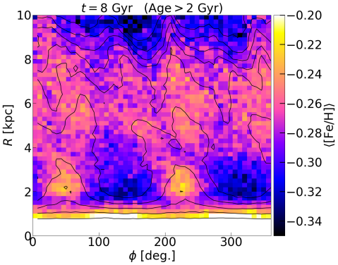
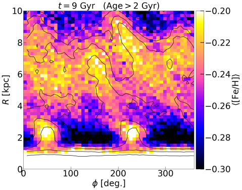
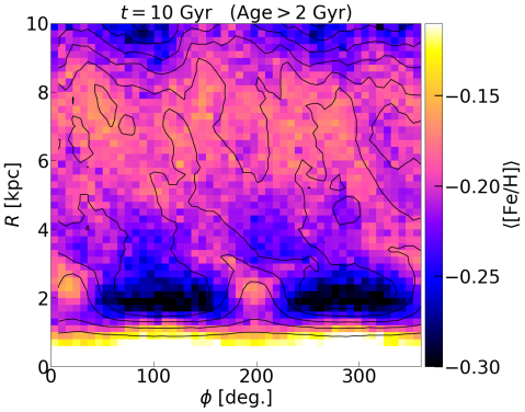
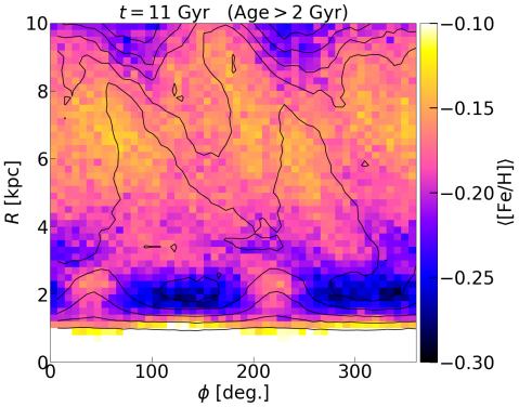
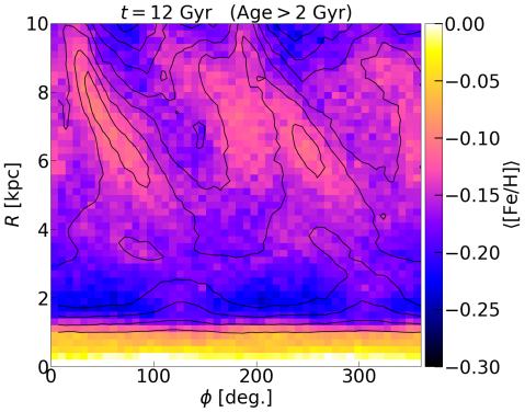
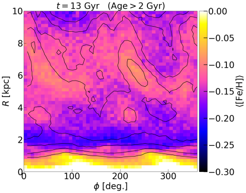
Figure 23: $\left<{\mbox{$\rm[Fe/H]$}}\right>$ in cylindrical coordinates at $t=8-13\mbox{$\>{\rm Gyr}$}$, as labelled. Only stars older than $2\mbox{$\>{\rm Gyr}$}$ are considered (compare Fig. 1). The contours correspond to the full surface density. Note the changing colour scale.

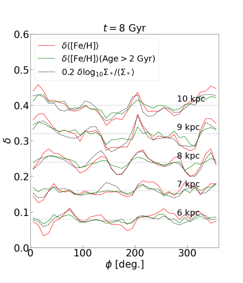
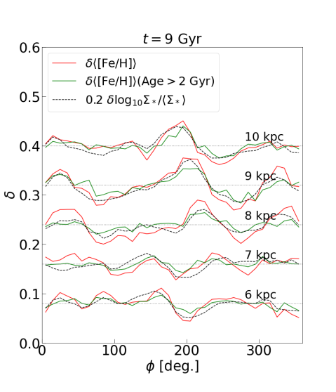
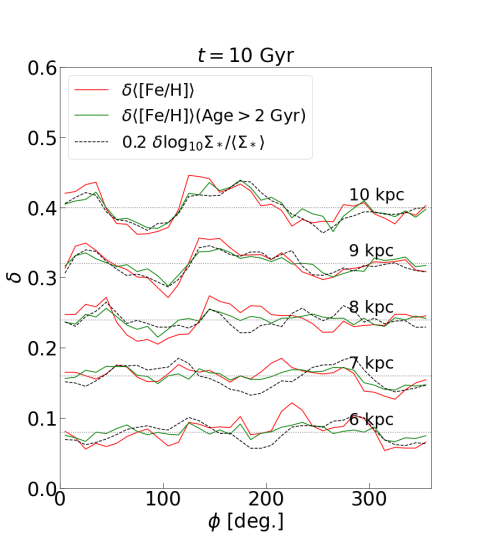
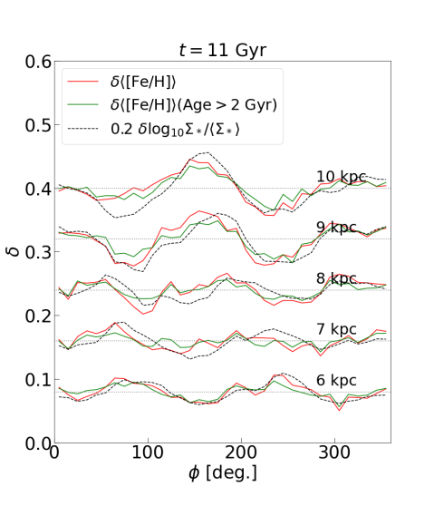
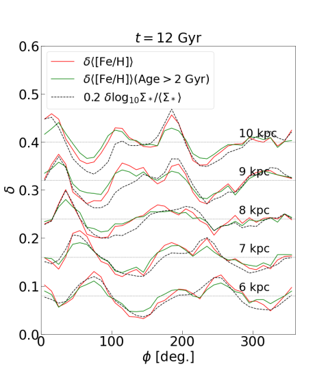
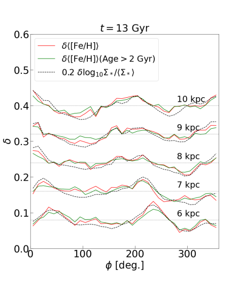
Figure 24: Same as the left panel of Fig. 2 at $t=8-13\mbox{$\>{\rm Gyr}$}$, as labelled.

References

- Al Kazwini et al. (2022) Al Kazwini, H., et al. 2022, A&A, 658, A50
- Bellardini et al. (2022) Bellardini, M. A., Wetzel, A., Loebman, S. R., & Bailin, J. 2022, MNRAS, 514, 4270
- Bellardini et al. (2021) Bellardini, M. A., Wetzel, A., Loebman, S. R., Faucher-Giguère, C.-A., Ma, X., & Feldmann, R. 2021, MNRAS, 505, 4586
- Binney (2012) Binney, J. 2012, MNRAS, 426, 1324
- Binney (2016) Binney, J. 2016, MNRAS, 462, 2792
- Binney (2018) Binney, J. 2018, MNRAS, 474, 2706
- Binney (2020) Binney, J. 2020, MNRAS, 495, 886
- Binney & McMillan (2011) Binney, J., & McMillan, P. 2011, MNRAS, 413, 1889
- Binney & Tremaine (2008) Binney, J., & Tremaine, S. 2008, Galactic Dynamics: Second Edition (Galactic Dynamics: Second Edition, by James Binney and Scott Tremaine. ISBN 978-0-691-13026-2 (HB). Published by Princeton University Press, Princeton, NJ USA, 2008.)
- Bland-Hawthorn & Gerhard (2016) Bland-Hawthorn, J., & Gerhard, O. 2016, ARAA, 54, 529
- Bovy et al. (2014) Bovy, J., et al. 2014, ApJ, 790, 127
- Carr et al. (2022) Carr, C., Johnston, K. V., Laporte, C. F. P., & Ness, M. K. 2022, MNRAS, 516, 5067
- Chiba et al. (2021) Chiba, R., Friske, J. K. S., & Schönrich, R. 2021, MNRAS, 500, 4710
- Di Matteo et al. (2013) Di Matteo, P., Haywood, M., Combes, F., Semelin, B., & Snaith, O. N. 2013, A&A, 553, A102
- Drimmel et al. (2023) Drimmel, R., et al. 2023, A&A, 670, A10
- Fiteni et al. (2021) Fiteni, K., Caruana, J., Amarante, J. A. S., Debattista, V. P., & Beraldo e Silva, L. 2021, MNRAS, 503, 1418
- Frankel et al. (2020) Frankel, N., Sanders, J., Ting, Y.-S., & Rix, H.-W. 2020, ApJ, 896, 15
- Gaia Collaboration et al. (2018) Gaia Collaboration, et al. 2018, A&A, 616, A11
- Ghosh et al. (2022) Ghosh, S., Debattista, V. P., & Khachaturyants, T. 2022, MNRAS, 511, 784
- Grand et al. (2016a) Grand, R. J. J., Springel, V., Gómez, F. A., Marinacci, F., Pakmor, R., Campbell, D. J. R., & Jenkins, A. 2016a, MNRAS, 459, 199
- Grand et al. (2016b) Grand, R. J. J., et al. 2016b, MNRAS, 460, L94
- Hawkins (2023) Hawkins, K. 2023, MNRAS, 525, 3318
- Ho et al. (2018) Ho, I. T., et al. 2018, A&A, 618, A64
- Hopkins et al. (2018) Hopkins, P. F., et al. 2018, MNRAS, 480, 800
- Hwang et al. (2019) Hwang, H.-C., et al. 2019, ApJ, 872, 144
- Imig et al. (2023) Imig, J., et al. 2023, ApJ, 954, 124
- Kawata et al. (2021) Kawata, D., Baba, J., Hunt, J. A. S., Schönrich, R., Ciucă, I., Friske, J., Seabroke, G., & Cropper, M. 2021, MNRAS, 508, 728