Tight (Double) Exponential Bounds for Identification Problems: Locating-Dominating Set and Test Cover

Abstract

We investigate fine-grained algorithmic aspects of identification problems in graphs and set systems, with a focus on Locating-Dominating Set and Test Cover. In the first problem, an input is a graph $G$ on $n$ vertices and an integer $k$, and the objective is to decide whether there is a subset $S$ of $k$ vertices such that every vertex not in $S$ is dominated by a unique subset of $S$. In the second problem, an input is a set of items $U$, a collection of subsets $\mathcal{F}$ of $U$ called tests, and an integer $k$, and the objective is to select at most $k$ tests such that for each pair of items, there is a test that contains exactly one of the two items. We prove, among other things, the following three (tight) conditional lower bounds.

1. Locating-Dominating Set does not admit an algorithm running in time $2^{o(k^{2})}\cdot poly(n)$, nor a polynomial time kernelization algorithm that reduces the solution size and outputs a kernel with $2^{o(k)}$ vertices, unless the ETH fails.

To the best of our knowledge, Locating-Dominating Set is the first problem that admits such an algorithmic lower-bound (with a quadratic function in the exponent) when parameterized by the solution size. The other such results known to us are for structural parameterizations like vertex cover [Agrawal et al., ACM Trans. Comput. Theory 2019; Foucaud et.al., arXiv 2023] or pathwidth [M. Pilipczuk, MFCS 2011; Sau and Souza, Inf. Comput., 2021].

1. Test Cover does not admit an algorithm running in time $2^{2^{o(k)}}\cdot poly(|U|+|\mathcal{F}|)$.

After Edge Clique Cover [Cygan et al., SIAM J. Comput. 2016] and BiClique Cover [Chandran et al., IPEC 2016], this is the only example that we know of that admits a double exponential lower bound when parameterized by the solution size.

1. Locating-Dominating Set (respectively, Test Cover) parameterized by the treewidth of the input graph (respectively, of the natural auxiliary graph) does not admit an algorithm running in time $2^{2^{o(\textsf{tw})}}\cdot poly(n)$ (respectively, $2^{2^{o(\textsf{tw})}}\cdot poly(|U|+|\mathcal{F}|))$.

This result augments the small list of NP-Complete problem that admit double exponential lower bounds when parameterized by treewidth [Foucaud et al. arXiv 2023; Chalopin et al. arXiv 2023].

We also present algorithms whose running times match the above lower bounds. We also investigate the incompressibility of these problems, and parameterizations by several other structural graph parameters, such as vertex cover number and feedback edge set number. Our results regarding these parameters answer some open problems from the literature.

1 Introduction

The aim of this paper is to study the algorithmic properties of certain identification problems in discrete structures. In identification problems, one wishes to select a solution substructure of an input structure (subset of vertices, coloring of a graph, etc) so that each element is uniquely identified by the solution substructure. Some well-studied examples are for example the problems Test Cover for set systems, Metric Dimension for graphs (Problem [SP6] and [GT61] in the book by Garey and Johnson [33], respectively). This type of problems is studied since the 1960s both in the combinatorics community (see e.g. Rényi [51] or Bondy [8]), and in the algorithms community since the 1970s [7, 9, 22, 47]. They have multiple practical and theoretical applications; such as network monitoring [50], medical diagnosis [47], bioinformatics [7], graph isomorphism [4], or machine learning [16], to name a few.

First, we focus on one graph problem of the area, Locating-Dominating Set (that can be seen as a local version of Metric Dimension), which is also a graph domination problem. We study its algorithmic properties with respect to various parameterizations of the inputs, such as the solution size or structural parameters of the input graph. In the classic Dominating Set problem, an input is an undirected graph $G$ and an integer $k$, and the objective is to decide whether there exists a subset $S\subseteq V(G)$ such that for any vertex $u\in V(G)\setminus S$, at least one of its neighbours is in $S$. Locating-Dominating Set is a variant of this problem which was introduced by Slater in the 1980s [53, 55], and is defined as follows.

Locating-Dominating Set Input: A graph $G$ on $n$ vertices and an integer $k$ Question: Does there exist a locating-dominating set of size $k$ in $G$, that is, a dominating set $S$ of $G$ such that for any two different vertices $u,v\in V(G)\setminus S$, their neighbourhoods in $S$ are different, i.e., $N(u)\cap S\neq N(v)\cap S$?

We demonstrate the applicability of our key ideas by proving corresponding results about Test Cover. As this problem is defined over set systems, for structural parameters, we define an auxiliary graph in the natural way, as follows.

Test Cover Input: A set of items $U$, a collection of subsets of $U$ called tests and denoted by $\mathcal{F}$, and an integer $k$. Question: Does there exist a collection of at most $k$ tests such that for each pair of items, there is a test that contains exactly one of the two items? Auxiliary Graph: A bipartite graph $G$ on $n$ vertices with bipartition $\langle R,B\rangle$ of $V(G)$ such that sets $R$ and $B$ contain a vertex for every set in $\mathcal{F}$ and for every item in $U$, respectively, and $r\in R$ and $b\in B$ are adjacent if and only if the set corresponding to $r$ contains the element corresponding to $b$.

Locating-Dominating Set and Test Cover are both -complete (see [33] and [17]). They are also trivially  for the parameter solution size. Indeed, as any solution must have size at least logarithmic in the number of elements/vertices (assuming no redundancy in the input), the whole instance is a trivial single-exponential kernel for Locating-Dominating Set, and double-exponential in the case of Test Cover. Hence, it becomes interesting to study these problems under more refined angles, such as kernelization, fine-grained complexity, and alternative parameterizations. Naturally, these lines of research have been pursued in the literature. For the case of Test Cover, “above/below guarantee” parameterizations were studied in [6, 21, 22, 35] and kernelization in [6, 21, 35]. These results have shown an intriguing behaviour for Test Cover, with some nontrivial techniques being developed to solve the problem [6, 22]. In the case of Locating-Dominating Set, structural parameterizations of the input graph have been studied in [10, 11], and fine-grained complexity results regarding the number of vertices and solution size were obtained in [5, 10]. Refer to the “related work” section at the end of the introduction, for a more detailed overview.

We extend the above results by systematically studying the fine-grained complexity and kernelization of Locating-Dominating Set and Test Cover for parameters solution size, number of vertices/elements/tests, and structural parameters. We obtain tight ETH-based lower bounds, complemented by algorithms with matching running times. We also complete the picture for structural parameterizations of Locating-Dominating Set started in [11] (and obtain similar results for the natural auxiliary graphs defined over the inputs of Test Cover).

Our bounds show that the running times for these two problems are highly nontrivial, exhibiting interesting runtime functions that appear to be quite rare in the literature, whether for the solution size or structural parameters like the treewidth. This confirms the interesting algorithmic nature of identification problems.

Incompressibility Results.

It is known that for the Dominating Set problem, there is no polynomial-time algorithm that reduces any $n$-vertex input to an equivalent instance (of an arbitrary problem), with bit-size $\mathcal{O}(n^{2-\epsilon})$ for every $\epsilon>0$, unless $\NP\subseteq\coNP/poly$ [40]. We prove a similar result for Locating-Dominating Set.

Theorem 1.1.

Neither Locating-Dominating Set nor Test Cover admits a polynomial compression of size $\mathcal{O}(n^{2-\epsilon})$ for any $\epsilon>0$, unless $\NP\subseteq\coNP/poly$.

The reduction used to prove Theorem 1.1 also yields the following results. First, it proves that Locating-Dominating Set, parameterized by the vertex cover number of the input graph and the solution size, does not admit a polynomial kernel, unless $\NP\subseteq\coNP/poly$. Our reduction is arguably a simpler argument than the one present in [10] to obtain the same result. Second, it proves that Test Cover, parameterized by the number of items $|U|$ and the solution size $k$, does not admit a polynomial kernel, unless $\NP\subseteq\coNP/poly$. Additionally, it also implies that Test Cover, parameterized by the number of sets $|\mathcal{F}|$, does not admit a polynomial kernel, unless $\NP\subseteq\coNP/poly$. This improves upon the result in [35], that states that there is no polynomial kernel for the problem when parameterized by $k$ alone. Note that Test Cover admits a simple exponential kernel when parameterized by the number of vertices (alone) or by the number of sets (alone).

Solution Size as Parameter.

Dominating Set is a canonical $\W[2]$-Complete problem, when parameterized by solution size $k$. In contrast, Locating-Dominating Set admits a trivial kernel with size $\mathcal{O}(2^{k})$, and hence, an  algorithm running in time $2^{\mathcal{O}(k^{2})}$. We prove that both of these bounds are optimal.

Theorem 1.2.

Unless the ETH fails, Locating-Dominating Set, parameterized by the solution size $k$, does not admit

• a polynomial time kernelization algorithm that reduces the solution size and outputs a kernel with $2^{o(k)}$ vertices, nor

• an algorithm running in time $2^{o(k^{2})}\cdot n^{\mathcal{O}(1)}$.

This type of result seems to be quite rare in the literature. The only results known to us about ETH-based conditional lower bounds on the number of vertices in a kernel are for Edge Clique Cover [23], Biclique Cover [13], Metric Dimension and two related problems [29]. Regarding the second result, to the best of our knowledge, Locating-Dominating Set becomes the first known problem to admit such a lower bound, with a matching upper bound, when parameterized by the solution size. The only other problems known to us, admitting similar lower bounds, are for structural parameterizations like vertex cover [1, 12, 29] or pathwidth [49, 52]. Theorem 1.2 also improves upon a “no $2^{\mathcal{O}(k)}n^{\mathcal{O}(1)}$ algorithm” bound from [5] (under $\W[2]\neq\FPT$) and a $2^{o(k\log k)}$ ETH-based lower bound recently proved in [10].

Now, consider the case of Test Cover. As mentioned before, it is safe to assume that $|\mathcal{F}|\leq 2^{|U|}$ and $|U|\leq 2^{k}$. By Bondy’s theorem [8], we can also assume that $k\leq|U|-1$. Hence, the brute-force algorithm that enumerates all the sub-colletions of tests of size at most $k$ runs in time $|\mathcal{F}|^{\mathcal{O}(|U|)}=2^{\mathcal{O}(|U|^{2})}=2^{2^{\mathcal{O}(k)}}$. Our next result proves that this simple algorithm is again optimal.

Theorem 1.3.

Test Cover does not admit an algorithm running in time $2^{2^{o(k)}}\cdot(|U|+|\mathcal{F}|)^{\mathcal{O}(1)}$, unless the ETH fails.

The lower bound of Theorem 1.3 is only the third such double-exponential lower bound for solution size, known to us. The other known ones are for Edge Clique Cover [23] and BiClique Cover [13]

Treewidth as Parameter.

At this point, it is tempting to assert that Locating-Dominating Set  is “easier” than Dominating Set in the realm of parameterized complexity. Even if this is true in the case of the natural parameterization by solution size, our next result shows that this is not the case for structural parameterizations.

Theorem 1.4.

Both Locating-Dominating Set and Test Cover, parameterized by the treewidth tw of the input graph and the auxiliary graph, respectively, admit algorithms running in time $2^{2^{\mathcal{O}(\textsf{tw})}}\cdot n^{\mathcal{O}(1)}$. However, unless the ETH fails, none of them admits an algorithm running in time $2^{2^{o(\textsf{tw})}}\cdot n^{\mathcal{O}(1)}$.

We remark that the algorithmic lower bound of Theorem 1.4 holds true even with respect to tree-depth, a larger parameter than treewidth.

Recall that, in contrast, Dominating Set admits an algorithm running in time $\mathcal{O}(3^{\textsf{tw}}\cdot n^{2})$ [58, 46]. Theorem 1.4 adds Locating-Dominating Set and Test Cover to the short list of  problems that admit (tight) double-exponential lower bounds for structural graph parameters. Recently, three distance-related graph problems in  (Metric Dimension, Strong Metric Dimension, Geodetic Set) were shown in [29] to admit such lower bounds for parameters treewidth and vertex cover number. Using similar techniques as [29], two problems from learning theory were shown in [12] to admit similar lower bounds: Non-Clashing Teaching Map and Non-Clashing Teaching Dimension. We continue to demonstrate the applicability of the techniques from [29] to yet another type of problems (local identification problems), namely Locating-Dominating Set and Test Cover. We adapt the main technique developed in [29] to our setting, namely, the bit-representation gadgets.

Other Structural Parameters.

Our next result shows that the lower bound of Theorem 1.4 (for treewidth and even tree-depth) cannot be obtained for the even larger parameter vertex cover number.

Theorem 1.5.

Locating-Dominating Set admits $(i)$ algorithm running in time $2^{\mathcal{O}(\textsf{vc}\log\textsf{vc})}\cdot n^{\mathcal{O}(1)}$, $(ii)$ a kernel with $\mathcal{O}(\textsf{nd})$ vertices, and $(iii)$ a kernel with $\mathcal{O}(\textsf{fes})$ vertices. Here, vc, nd, and fes are the vertex cover number, neighbourhood diversity, and the feedback edge set number, respectively, of the input graph.

In fact, we also show that Theorem 1.5(i) extends to the parameters distance to clique and twin-cover number. Note that the reduction of Theorem 1.1 implies that Locating-Dominating Set cannot be solved in time $2^{o(n)}$, and thus, in time $2^{o(\textsf{vc})}$ (under the ETH), hence the bound of Theorem 1.5(i) is close to optimal. Theorem 1.5(iii) answers the main open problem raised in [10, 11], about the parameter feedback edge set number. See Figure 1 for an overview of the known results for (structural) parameterizations of Locating-Dominating Set, using a Hasse diagram of standard graph parameters.

Regarding Test Cover, using the same idea as for the algorithm from Theorem 1.5(i), we also obtain the following result, which is reminiscent of the known $\mathcal{O}(mn2^{n})$ dynamic programming scheme for Set Cover on a universe of size $n$ and $m$ sets (see [26, Theorem 3.10]), and improves upon the naive $2^{\mathcal{O}(|B|^{2})}\cdot(|R|+|B|)^{\mathcal{O}(1)}$ brute-force algorithm.

Theorem 1.6.

Test Cover can be solved in time $2^{\mathcal{O}(|B|\log|B|)}\cdot(|R|+|B|)^{\mathcal{O}(1)}$.

Figure 1: Hasse diagram of graph parameters and associated results for Locating-Dominating Set. An edge from a lower parameter to a higher parameter indicates that the lower one is upper bounded by a function of the higher one. If the line is dashed, then the bound is exponential; otherwise, it is linear. Colors correspond to the known FPT complexity status with respect to the highlighted parameter: the upper half of the box represents the upper bound, and the lower half of the box represents the lower bound. By “single-exponential”, “slightly superexponential” and “double-exponential”, we mean functions of the form $2^{\mathcal{O}(p)}$, $2^{\mathcal{O}(p\log p)}$ or $2^{\mathcal{O}(p^{2})}$, and $2^{2^{\mathcal{O}(p)}}$, respectively. The parameters for which the running time is not known to be tight are thus striped. The red circle in the upper-right corner means that Locating-Dominating Set does not admit a polynomial kernel when parameterized by the marked parameter unless $\NP\subseteq\coNP/poly$; the yellow one means that a (tight) quadratic kernel exists, and the green one, that a linear kernel exists. The bold borders highlight parameters that are covered in this paper.

Organization.

We use the Locating-Dominating Set problem to demonstrate key technical concepts regarding lower bounds and algorithms. The arguments regarding Test Cover follows almost the identical line. We present detailed arguments about Locating-Dominating Set in Section 3 to 6, and then mention the modification needed for Test Cover in Section 7. We conclude the paper with some open problems in Section 8.

Related work.

Test Cover was shown to be -complete by Garey and Johnson [33, Problem SP6] and it is also hard to approximate within a ratio of $(1-\epsilon)\ln n$ [9] (an approximation algorithm with ratio $1+\ln n$ exists by reduction to Set Cover [7]). As any solution has size at least $\log_{2}(n)$, the problem admits a trivial kernel of size $2^{2^{k}}$, and thus Test Cover is FPT parameterized by solution size $k$. Parameterizations from the “above/below guarantee” framework have been studied: Test Cover is FPT for parameters $n-k$, but $W[1]$-hard for parameters $m-k$ and $k-\log_{2}(n)$ [22]. However, assuming standard assumptions, there is no polynomial kernel for the parameterizations by $k$ and $n-k$ [35], although there exists a “partially polynomial kernel” for parameter $n-k$ [6] (i.e. one with $O((n-k)^{7})$ elements, but potentially exponentially many tests). When the tests have all a fixed upper bound $r$ on their size, the parameterizations by $k$, $n-k$ and $m-k$ all become FPT with a polynomial kernel [21, 35].

The problem Discriminating Code [14] is very similar to Test Cover (with the distinction that the input is presented as a bipartite graph, one part representing the elements and the other, the tests, and that every element has to be covered by some solution test), and has been shown to be -complete even for planar instances [15].

Locating-Dominating Set is -complete [17], even for special graph classes such as planar unit disk graphs [48], planar bipartite subcubic graphs, chordal bipartite graphs, split graphs and co-bipartite graphs [28], interval and permutation graphs of diameter 2 [31]. For the same reason as for Test Cover, Locating-Dominating Set has a trivial kernel with $2^{k}+k$ vertices. By a straightforward application of Courcelle’s theorem [19], Locating-Dominating Set is FPT for parameter treewidth and even cliquewidth [20]. Explicit polynomial-time algorithms were given for trees [53], block graphs [3], series-parallel graphs [17], and cographs [30]. Regarding the approximation complexity of Locating-Dominating Set, similar results as for Test Cover have been obtained for Locating-Dominating Set, see [28, 34, 56].

It was shown in [5] that Locating-Dominating Set cannot be solved in time $2^{o(n)}$ on bipartite graphs, nor in time $2^{o(\sqrt{n})}$ on planar bipartite graphs or on apex graphs, assuming the ETH. Moreover, they also showed that Locating-Dominating Set cannot be solved in time $2^{\mathcal{O}(k)}n^{\mathcal{O}(1)}$ on bipartite graphs, unless $\W[2]=\FPT$. Note that the authors of [5] have designed a complex framework with the goal of studying a large class of identification problems related to Locating-Dominating Set and similar problems.

In [11], structural parameterizations of Locating-Dominating Set were studied. It was shown that the problem admits a linear kernel for the parameter max leaf number, however (under standard complexity assumptions) no polynomial kernel exists for the solution size, combined with either the vertex cover number or the distance to clique. They also provide a double-exponential kernel for the parameter distance to cluster. In the full version [10] of [11], the same authors show that Locating-Dominating Set does neither admit a $2^{o(k\log k)}n^{\mathcal{O}(1)}$-time nor an $n^{o(k)}$-time algorithm, assuming the ETH.

2 Preliminaries

For a positive integer $q$, we denote the set $\{1,2,\dots,q\}$ by $[q]$. We use $\mathbb{N}$ to denote the collection of all non-negative integers.

Graph theory

We use standard graph-theoretic notation, and we refer the reader to [25] for any undefined notation. For an undirected graph $G$, sets $V(G)$ and $E(G)$ denote its set of vertices and edges, respectively. We denote an edge with two endpoints $u,v$ as $uv$. Unless otherwise specified, we use $n$ to denote the number of vertices in the input graph $G$ of the problem under consideration. Two vertices $u,v$ in $V(G)$ are adjacent if there is an edge $uv$ in $G$. The open neighborhood of a vertex $v$, denoted by $N_{G}(v)$, is the set of vertices adjacent to $v$. The closed neighborhood of a vertex $v$, denoted by $N_{G}[v]$, is the set $N_{G}(v)\cup\{v\}$. We say that a vertex $u$ is a pendant vertex if $|N_{G}(v)|=1$. We omit the subscript in the notation for neighborhood if the graph under consideration is clear. For a subset $S$ of $V(G)$, we define $N[S]=\bigcup_{v\in S}N[v]$ and $N(S)=N[S]\setminus S$. For a subset $S$ of $V(G)$, we denote the graph obtained by deleting $S$ from $G$ by $G-S$. We denote the subgraph of $G$ induced on the set $S$ by $G[S]$.

Locating-Dominating Sets

A subset of vertices $S$ in graph $G$ is called its dominating set if $N[S]=V(G)$. A dominating set $S$ is said to be a locating-dominating set if for any two different vertices $u,v\in V(G)\setminus S$, we have $N(u)\cap S\neq N(v)\cap S$. In this case, we say vertices $u$ and $v$ are distinguished by the set $S$. We say a vertex $u$ is located by set $S$ if for any vertex $v\in V(G)\setminus\{u\}$, $N(u)\cap S\neq N(v)\cap S$. We note the following simple observation.

If set $S\subseteq V(G)$ locates $u$, then any set $S^{\prime}$ such that $S\subseteq S^{\prime}\subseteq V(G)$ also locates $u$.

Proof 2.1.

Assume for the sake of contradiction that $S^{\prime}$ does not locate $u$, i.e., there is a vertex $v\in V(G)\setminus\{u\}$ such that $N(u)\cap S^{\prime}=N(v)\cap S^{\prime}$. As $S\subseteq S^{\prime}$, this implies $N(u)\cap S=N(v)\cap S$, contradicting the fact that $S$ locates $v$. Hence, once a set locates a vertex, any of its supersets locates that vertex.

Next, we prove that it is safe to consider the locating-dominating set that contains all the vertices adjacent with pendant vertices.

Consider a vertex $v$ which is adjacent with a pendant vertex in $G$. If $S$ is a locating-dominating set of $G$, then there is a locating-dominating set $S^{\prime}$ of $G$ such that $|S^{\prime}|\leq|S|$ and $v\in S^{\prime}$.

Proof 2.2.

Let $u$ be a pendant vertex which is adjacent with $v$. As $S$ is a (locating) dominating set, we have $\{u,v\}\cap S\neq\emptyset$. Suppose $u\in S$ and $v\not\in S$. Define $S^{\prime}=(S\cup\{v\})\setminus\{u\}$. It is easy to see that $S^{\prime}$ is a dominating set. If $S^{\prime}$ is not a locating-dominating set, then there exists $w$, apart from $u$, in the neighbourhood of $v$ such that both $u$ and $w$ are adjacent with only $v$ in $S^{\prime}$. As $u$ is a pendant vertex and $v$ its unique neighbour, $w$ is not adjacent with $u$. Hence, $w$ was not adjacent with any vertex in $S^{\prime}\setminus\{v\}=S\setminus\{u\}$. This, however, contradicts the fact that $S$ is a (locating) dominating set. Hence, $S^{\prime}$ is a locating-dominating set and $|S^{\prime}|=|S|$.

Parameterized complexity

An instance of a parameterized problem $\Pi$ consists of an input $I$, which is an input of the non-parameterized version of the problem, and an integer $k$, which is called the parameter. Formally, $\Pi\subseteq\Sigma^{*}\times\mathbb{N}$. A problem $\Pi$ is said to be fixed-parameter tractable, or , if given an instance $(I,k)$ of $\Pi$, we can decide whether $(I,k)$ is a Yes-instance of $\Pi$ in time $f(k)\cdot|I|^{\mathcal{O}(1)}$. Here, $f:\mathbb{N}\mapsto\mathbb{N}$ is some computable function depending only on $k$. Parameterized complexity theory provides tools to rule out the existence of  algorithms under plausible complexity-theoretic assumptions. For this, a hierarchy of parameterized complexity classes $\FPT\subseteq\W[1]\subseteq\W[2]\cdots\subseteq\XP$ was introduced, and it was conjectured that the inclusions are proper.

A parameterized problem $\Pi$ is said to admit a kernelization if given an instance $(I,k)$ of $\Pi$, there is an algorithm that runs in time polynomial in $|I|+k$ and constructs an instance $(I^{\prime},k^{\prime})$ of $\Pi$ such that (i) $(I,k)\in\Pi$ if and only if $(I^{\prime},k^{\prime})\in\Pi$, and (ii) $|I^{\prime}|+k^{\prime}\leq g(k)$ for some computable function $g:\mathbb{N}\mapsto\mathbb{N}$ depending only on $k$. If $g(\cdot)$ is a polynomial function, then $\Pi$ is said to admit a polynomial kernelization. In some cases, it is possible that a parameterized problem $\Pi$ is preprocessed into an equivalent instance of a different problem satisfying some special properties. Such preprocessing algorithms are also well-known in the literature. A polynomial compression of a parameterized problem $\Pi$ into a problem $\Psi\subseteq\Sigma^{*}$ is an algorithm that given an instance $(I,k)$ of $\Pi$, runs in polynomial in $|I|+k$ time, and outputs an instance $I^{\prime}$ of $\Psi$ such that (i) $(I,k)\in\Pi$ if and only if $I^{\prime}\in\Psi$, and (ii) $|I^{\prime}|\leq f(k)$ for a polynomial function $f:\mathbb{N}\mapsto\mathbb{N}$. If $|\Sigma|=2$, then the function $f(\cdot)$ is called the bitsize of the compression. A reduction rule is a polynomial-time algorithm that takes as input an instance of a problem and outputs another, usually reduced, instance. A reduction rule said to be applicable on an instance if the output instance and input instance are different. A reduction rule is safe if the input instance is a Yes-instance if and only if the output instance is a Yes-instance. For a detailed introduction to parameterized complexity and related terminologies, we refer the reader to the recent books by Cygan et al. [24] and Fomin et al. [27].

3 Incompressiblity of Locating-Dominating Set

In this section, we prove Thereom 1.1 for Locating-Dominating Set, i.e., we prove Locating-Dominating Set does not admit a polynomial compression of size $\mathcal{O}(n^{2-\epsilon})$ for any $\epsilon>0$, unless $\NP\subseteq\coNP/poly$. We transfer the incompressibility of Dominating Set to Locating-Dominating Set. It will be convenient to reduce from the Red-Blue Dominating Set problem, a restricted version of Dominating Set, which also does not admit a compression with $\mathcal{O}(n^{2-\epsilon})$ bits unless $\NP\subseteq\coNP/poly$ [2, Proposition 2].

Red-Blue Dominating Set Input: A bipartite graph $G^{\prime}$, a bipartition $\langle R^{\prime},B^{\prime}\rangle$ of $V(G^{\prime})$, and an integer $k^{\prime}$ Question: Does there exist a set $S^{\prime}\subseteq R^{\prime}$ such that $|S^{\prime}|\leq k^{\prime}$ and $S^{\prime}$ dominates $B^{\prime}$, i.e. $B^{\prime}\subseteq N(S^{\prime})$?

It is safe to assume that $G^{\prime}$ does not contain an isolated vertex. Indeed, if there is an isolated vertex in $R$, one can delete it to obtain an equivalent instance. If $B$ contains an isolated vertex, it is a trivial No-instance. Moreover, it is also safe to assume that $R^{\prime}\leq 2^{|B^{\prime}|}$ as it is safe to remove one of the two false twins in $R^{\prime}$. Also, $k^{\prime}\leq|B^{\prime}|$ as otherwise given instance is a trivial Yes-instance.

Reduction

The reduction takes as input an instance $(G^{\prime},\langle R^{\prime},B^{\prime}\rangle,k^{\prime})$ of Red-Blue Dominating Set and constructs an instance $(G,k)$ of Locating-Dominating Set. Suppose we have $R^{\prime}=\{r^{\prime}_{1},r^{\prime}_{2},\dots,r^{\prime}_{|R|}\}$ and $B^{\prime}=\{b^{\prime}_{1},b^{\prime}_{2},\dots,b^{\prime}_{|B|}\}$. The reduction constructs graph $G$ in the following steps. See Figure 2 for an illustration.

• It adds sets of vertices $R$ and $B$ to $G$, where $R$ contains a vertex corresponding to each vertex in $R^{\prime}$ and $B$ contains two vertices corresponding to each vertex in $B^{\prime}$. Formally, $R=\{r_{i}|\ i\in[|R^{\prime}|]\}$ and $B=\{b^{\circ}_{i},b^{\star}_{i}|\ i\in[|B^{\prime}|]\}$.

• The reduction adds a bit representation gadget to locate set $R$. Informally, it adds some supplementary vertices such that it is safe to assume these vertices are present in a locating-dominating set, and they locate every vertex in $R$.

  • First, set $q:=\lceil\log(|R|)\rceil+1$. This value for $q$ allows to uniquely represent each integer in $[|R|]$ by its bit-representation in binary when started from $1$ and not $0$.

  • For every $i\in[q]$, the reduction adds two vertices $y_{i,1}$ and $y_{i,2}$ and edge $(y_{i,1},y_{i,2})$.

  • For every integer $\ell\in[|R|]$, let $\texttt{bit}(\ell)$ denotes the binary representation of $\ell$ using $q$ bits. It connects $a_{\ell}\in R$ with $y_{i,1}$ if the $i^{th}$ bit (going from left to right) in $\texttt{bit}(\ell)$ is $1$.

  • It adds two vertices $y_{0,1}$ and $y_{0,2}$, and edge $(y_{0,1},y_{0,2})$, and makes every vertex in $R$ adjacent with $y_{0,1}$.

    Let $\texttt{bit-rep}(R)$ be the collection of all the vertices added in this step.

• Similarly, the reduction adds a bit representation gadget to locate set $B$. However, it adds vertices such that for any pair $b^{\circ}_{j},b^{\star}_{j}$, the supplementary vertices adjacent to them are identical.

  • The reduction sets $p:=\lceil\log(|B|/2)\rceil+1$ and for every $i\in[p]$, it adds two vertices $z_{i,1}$ and $z_{i,2}$ and edge $(z_{i,1},z_{i,2})$.

  • For every integer $j\in[|B|/2]$, let $\texttt{bit}(j)$ denote the binary representation of $j$ using $q$ bits. Connect $b^{\circ}_{j},b^{\star}_{j}\in B$ with $z_{i,1}$ if the $i^{th}$ bit (going from left to right) in $\texttt{bit}(j)$ is $1$.

  • It add two vertices $z_{0,1}$ and $z_{0,2}$, and edge $(z_{0,1},z_{0,2})$. It also makes every vertex in $B$ adjacent with $z_{0,1}$.

    Let $\texttt{bit-rep}(B)$ be the collection of all the vertices added in this step.

• Finally, the reduction adds edges across $R$ and $B$ as follows: For every pair of vertices $r^{\prime}_{i}\in R^{\prime}$ and $b^{\prime}_{j}\in B^{\prime}$,

  • if $r^{\prime}_{i}$ is not adjacent with $b^{\prime}_{j}$ then it adds both edges $(r_{i},b^{\circ}_{j})$ and $(r_{i},b^{\star}_{j})$ to $E(G)$, and

  • if $r^{\prime}_{i}$ is adjacent with $b^{\prime}_{j}$ then it adds $(r_{i},b^{\circ}_{j})$ only, i.e., it does not add an edge with endpoints $r_{i}$ and $b^{\star}_{j}$.

This completes the construction of $G$. The reduction sets

$$k=k^{\prime}+|\texttt{bit-rep}(R)|+|\texttt{bit-rep}(B)|=k^{\prime}+\log(|R|)+1+1+\log(|B|/2)+1+1,$$

and returns $(G,k)$ as an instance of Locating-Dominating Set.

Figure 2: An illustrative example of the graph constructed by the reduction. Adjacency to $y_{1,1}$, $y_{2,1}$, $y_{3,1}$ correspond to $1$ in the bit representation from left to right (most significant to least significant) bits. In the above example, the bit representation of $r_{1}$ is $\langle 1,0,0\rangle$, $r_{2}$ is $\langle 0,1,0\rangle$, $r_{3}$ is $\langle 1,1,0\rangle$, etc. For brevity, we only show the edges incident on $r_{3}$. The dotted line represents a non-edge. In this example, $r^{\prime}_{3}$ is only adjacent to $b^{\prime}_{2}$ in $G^{\prime}$. It is easy to see that $r_{3}$ can only resolve pair $(b^{\circ}_{2},b^{\star}_{2})$.

Lemma 3.1.

$(G^{\prime},\langle R^{\prime},B^{\prime}\rangle,k^{\prime})$ is a Yes-instance of Red-Blue Dominating Set if and only if $(G,k)$ is a Yes-instance of Locating-Dominating Set.

Proof 3.2.

$(\Rightarrow)$ Suppose $(G^{\prime},\langle R^{\prime},B^{\prime}\rangle,k^{\prime})$ is a Yes-instance and let $S^{\prime}\subseteq R^{\prime}$ be a solution. We prove that $S=S^{\prime}\cup\texttt{bit-rep}(R)\cup\texttt{bit-rep}(B)$ is a locating-dominating set of size at most $k$. The size bound follows easily. By the property of a set representation gadget, every vertex in $R$ is adjacent with a unique set of vertices in $\texttt{bit-rep}(R)\setminus\{z_{0,1}\}$. Consider a vertex $r_{i}$ in $R$ such that the bit-representation of $i$ contains a single $1$ at $j^{th}$ location. Hence, $z_{j,2}$ and $r_{i}$ are adjacent with the same vertex, viz $z_{j,1}$ in $\texttt{bit-rep}(R)\setminus\{z_{0,1}\}$. However, this pair of vertices is resolved by $z_{0,1}$ which is adjacent with $r_{i}$ and not with $z_{j,2}$. Also, as the bit-representation of vertices starts from $1$, there is no vertex in $R$ which is adjacent with only $z_{0,1}$ in $\texttt{bit-rep}(R)$. Using similar arguments and the properties of the set representation gadget, we can conclude that $\texttt{bit-rep}(R)\cup\texttt{bit-rep}(B)$ resolves all pairs of vertices, apart from those pairs of the form $(b^{\circ}_{j},b^{\star}_{j})$.

By the construction of $G$, a vertex $r_{i}\in R$ resolves a pair vertices $b_{j}^{\circ}$ and $b_{j}^{\star}$ if and only if $r^{\prime}_{i}$ and $b^{\prime}_{j}$ are adjacent. Since $S^{\prime}$ dominates $B$, $S^{\prime}$ resolves every pair of the form $(b_{j}^{\circ},b_{j}^{\star})$. Hence, $S^{\prime}\cup\texttt{bit-rep}(R)\cup\texttt{bit-rep}(B)$ is a locating-dominating set of $G$ of the desired size.

$(\Leftarrow)$ Suppose $S$ is a locating-dominating set of $G$ of size at most $k$. By Observation 2, it is safe to consider that $S$ contains $\texttt{bit-rep}(R)\cup\texttt{bit-rep}(B)$, as every vertex in it is adjacent to a pendant vertex. Next, we modify $S$ to obtain another locating-dominating set $S_{1}$ such that $|S_{1}|\leq|S|$ and all vertices in $S_{1}\setminus(\texttt{bit-rep}(R)\cup\texttt{bit-rep}(B))$ are in $R$. Without loss of generality, suppose $b^{\circ}_{j}\in S$. As discussed in the previous paragraph, $\texttt{bit-rep}(R)\cup\texttt{bit-rep}(B)$ resolves all the pair of vertices apart from the pair of the form $(b_{j^{\prime}}^{\circ},b_{j^{\prime}}^{\star})$. As there is no edge between the vertices in $B$, if $b^{\circ}_{j}\in S$ then it is useful only to resolve the pair $(b_{j}^{\circ},b_{j}^{\star})$. As there is no isolated vertex in $G^{\prime}$, every vertex in $B^{\prime}$ is adjacent with some vertex in $R^{\prime}$. Hence, by the construction of $G$, there is a vertex $r_{i}$ in $R$ such that $r_{i}$ is adjacent with $b^{\circ}_{j}$ but not with $b^{\star}_{j}$. Consider set $S_{1}=(S\setminus\{b_{j}^{\circ}\})\cup{r_{i}}$. By the arguments above, $|S_{1}|\leq|S|$, $S_{1}$ is a locating-dominating set of $G$, and $|S_{1}\cap B|<|S\cap B|$. Repeating this step, we obtain set $S_{1}$ with desired properties. It is easy to verify that $|S_{1}\cap R|=|S_{1}\cap R^{\prime}|\leq k^{\prime}$ and that for every vertex $b_{j}$ in $B^{\prime}$, there is a vertex in $S_{1}\cap R^{\prime}$ which is adjacent with $b_{j}$. Hence, the size of $S_{1}\cap R$ is at most $k$, and it dominates every vertex in $B$.

Proof 3.3 (Proof of Theorem 1.1).

Suppose there exists a polynomial-time algorithm $\mathcal{A}$ that takes as input an instance $(G,k)$ of Locating-Dominating Set and produces an equivalent instance $I^{\prime}$, which requires $\mathcal{O}(n^{2-\epsilon})$ bits to encode, of some problem $\Pi$. Consider the compression algorithm $\mathcal{B}$ for Red-Blue Dominating Set that uses the reduction mentioned in this section and then the algorithm $\mathcal{A}$ on the reduced instance. For an instance $(G^{\prime},\langle R^{\prime},B^{\prime}\rangle,k^{\prime})$ of Red-Blue Dominating Set, where the number of vertices in $G^{\prime}$ is $n^{\prime}$, the reduction constructs a graph $G$ with at most $3n^{\prime}$ vertices. Hence, for this input algorithm, $\mathcal{B}$ constructs an equivalent instance with $\mathcal{O}(n^{\prime 2-\epsilon})$ bits, contradicting $\NP\subseteq\coNP/poly$ [2, Proposition 2]. Hence, Locating-Dominating Set does not admit a polynomial compression of size $\mathcal{O}(n^{2-\epsilon})$ for any $\epsilon>0$, unless $\NP\subseteq\coNP/poly$.

Other Consequences of the Reduction.

Note that $\texttt{bit-rep}(R)\cup\texttt{bit-rep}(B)\cup B$ is a vertex cover of $G$ of size $\log(R)+\log(B)+|B|$. As $k^{\prime}\leq|B^{\prime}|$, $|R^{\prime}|\leq 2^{|B^{\prime}|}$, we have $\textsf{vc}(G)+k\leq(\log(R)+\log(B)+|B|)+k^{\prime}+\mathcal{O}(\log(R)+\log(B)+|B|)=\mathcal{O}(|B|)$. It is known that Red-Blue Dominating Set, parameterized by the number of blue vertices, does not admit a polynomial kernel unless $\NP\subseteq\coNP/poly$. See, for example, [24, Lemma $15.19$]. This, along with the arguments that are standard to parameter-preserving reductions, implies that Locating-Dominating Set, when parameterized jointly by the solution size and the vertex cover number of the input graph, does not admit a polynomial kernel unless $\NP\subseteq\coNP/poly$.

4 Locating-Dominating Set Parameterized by the Solution Size

In this section, we study the parameterized complexity of Locating-Dominating Set when parameterized by the solution size $k$. In the first subsection, we formally prove that the problem admits a kernel with $\mathcal{O}(2^{k})$ vertices, and hence a simple  algorithm running in time $2^{\mathcal{O}(k^{2})}$. In the second subsection, we prove that both results mentioned above are optimal under the ETH.

4.1 Upper bound

Proposition 4.1.

Locating-Dominating Set admits a kernel with $\mathcal{O}(2^{k})$ vertices and an algorithm running in time $2^{\mathcal{O}(k^{2})}+\mathcal{O}(k\log n)$.

Proof 4.2.

Slater proved that for any graph $G$ on $n$ vertices with a locating-dominating set of size $k$, we have $n\leq 2^{k}+k-1$ [55]. Hence, if $n>2^{k}+k-1$, we can return a trivial No instance (this check takes time $\mathcal{O}(k\log n)$). Otherwise, we have a kernel with $\mathcal{O}(2^{k})$ many vertices. In this case, we can enumerate all subsets of vertices of size $k$, and for each of them, check in quadratic time if it is a valid solution. Overall, this takes time ${n\choose k}n^{2}$; since $n\leq 2^{k}+k-1$, this is ${2^{\mathcal{O}(k)}\choose k}\cdot 2^{\mathcal{O}(k)}$, which is $2^{\mathcal{O}(k^{2})}$.

4.2 Lower Bound

In this section, we prove Theorem 1.2 which we restate.

See 1.2

Figure 3: An illustrative example of the graph constructed by the reduction. Suppose an instance $\psi$ of 3-SAT has $n=9$ variables and $4$ clauses. We do not show the third variable bucket and explicit edges across $A$ and $\texttt{bit-rep}(A)$ for brevity.

Reduction

To prove the theorem, we present a reduction that takes as input an instance $\psi$, with $n$ variables, of 3-SAT and returns an instance $(G,k)$ of Locating-Dominating Set such that $|V(G)|=2^{\mathcal{O}(\sqrt{n})}$ and $k=\mathcal{O}(\sqrt{n})$. By adding dummy variables in each set, we can assume that $\sqrt{n}$ is an integer. Suppose the variables are named $x_{i,j}$ for $i,j\in[\sqrt{n}]$. The reduction constructs graph $G$ as follows:

• It partitions the variables of $\psi$ into $\sqrt{n}$ many buckets $X_{1},X_{2},\dots,X_{\sqrt{n}}$ such that each bucket contains exactly $\sqrt{n}$ many variables. Let $X_{i}=\{x_{i,j}\ |\ j\in[\sqrt{n}]\}$ for all $i\in[\sqrt{n}]$.

  • For every $X_{i}$, it constructs set $A_{i}$ of $2^{\sqrt{n}}$ new vertices, $A_{i}=\{a_{i,\ell}\mid\ell\in[2^{\sqrt{n}}]\}$. Each vertex in $A_{i}$ corresponds to a unique assignment of variables in $X_{i}$. Let $A$ be the collection of all the vertices added in this step.

  • For every $X_{i}$, the reduction adds a path on three vertices $b^{\circ}_{i}$, $b^{\prime}_{i}$, and $b^{\star}_{i}$ with edges $(b^{\circ}_{i},b^{\prime}_{i})$ and $(b^{\prime}_{i},b^{\star}_{i})$. Suppose $B$ is the collection of all the vertices added in this step.

  • For every $X_{i}$, it makes $b^{\circ}_{i}$ adjacent with every vertex in $A_{i}$.

• For every clause $C_{j}$, the reduction adds a pair of vertices $c^{\circ}_{j},c^{\star}_{j}$. For a vertex $a_{\ell}\in A_{i}$ for some $i\in[\sqrt{n}]$, and $\ell\in[2^{\sqrt{n}}]$, if the assignment corresponding to vertex $a_{\ell}$ satisfies clause $C_{j}$, then it adds edge $(a_{\ell},c^{\circ}_{j})$.

• The reduction adds a bit-representation gadget to locate set $A$. Once again, informally speaking, it adds some supplementary vertices such that it is safe to assume these vertices are present in a locating-dominating set, and they locate every vertex in $A$. More precisely:

  • First, set $q:=\lceil\log(|A|)\rceil+1$. This value for $q$ allows to uniquely represent each integer in $[|A|]$ by its bit-representation in binary (starting from $1$ and not $0$).

  • For every $i\in[q]$, the reduction adds two vertices $y_{i,1}$ and $y_{i,2}$ and edge $(y_{i,1},y_{i,2})$.

  • For every integer $q^{\prime}\in[|A|]$, let $\texttt{bit}(q^{\prime})$ denotes the binary representation of $\ell$ using $q$ bits. Connect $a_{i,\ell}\in A$ with $y_{i,1}$ if the $i^{th}$ bit (going from left to right) in $\texttt{bit}((i+(\ell-1)\cdot\sqrt{n}))$ is $1$.

  • It adds two vertices $y_{0,1}$ and $y_{0,2}$, and edge $(y_{0,1},y_{0,2})$. It also makes every vertex in $A$ adjacent with $y_{0,1}$.

    Let $\texttt{bit-rep}(A)$ be the collection of all the vertices added in this step.

• Finally, the reduction adds a bit-representation gadget to locate set $C$. However, it adds the vertices in such a way that for any pair $c^{\circ}_{j},c^{\star}_{j}$, the supplementary vertices adjacent to them are identical.

  • The reduction sets $p:=\lceil\log(|C|/2)\rceil+1$ and for every $i\in[p]$, it adds two vertices $z_{i,1}$ and $z_{i,2}$ and edge $(z_{i,1},z_{i,2})$.

  • For every integer $j\in[|C|/2]$, let $\texttt{bit}(j)$ denotes the binary representation of $j$ using $q$ bits. Connect $c^{\circ}_{j},c^{\star}_{j}\in C$ with $z_{i,1}$ if the $i^{th}$ bit (going from left to right) in $\texttt{bit}(j)$ is $1$.

  • It add two vertices $z_{0,1}$ and $z_{0,2}$, and edge $(z_{0,1},z_{0,2})$. It also makes every vertex in $C$ adjacent with $y_{0,1}$.

    Let $\texttt{bit-rep}(C)$ be the collection of all the vertices added in this step.

This completes the reduction. The reduction sets

$$k=|B|/2+\log(|A|)+1+1+\lceil\log(|C|/2)\rceil+1+1+\sqrt{n}=\mathcal{O}(\sqrt{n})$$

as $|B|=2\sqrt{n}$, $|A|=\sqrt{n}\cdot 2^{\sqrt{n}}$, and $|C|=\mathcal{O}(n^{3})$, and returns $(G,k)$ as a reduced instance.

We present a brief overview of the proof of correctness in the reverse direction. Suppose $S$ is a locating-dominating set of graph $G$ of size at most $k$. Note that $b^{\star}_{i}$, $y_{i,2}$ and $z_{i,2}$ are pendant vertices for appropriate $i$. Hence, by Observation 2, it is safe to consider that vertices $b^{\prime}_{i}$, $y_{i,1}$, and $z_{i,1}$ are in $S$. This already forces $|B|/2+\log(|A|)+2+\lceil\log(|C|/2)\rceil+2$ many vertices in $S$. The remaining $\sqrt{n}$ many vertices need to locate vertices in pairs ($b^{\circ}_{i}$, $b^{\star}_{i}$) and $(c^{\circ}_{j}$, $c^{\star}_{j})$ for every $i\in[\sqrt{n}]$ and $j\in[|C|]$. Note that the only vertices that are adjacent with $b^{\circ}_{i}$ but are not adjacent with $b^{\star}_{i}$ are in $A_{i}$. Also, the only vertices that are adjacent with $c^{\circ}_{j}$ but are not adjacent with $c^{\star}_{j}$ are in $A_{i}$ and correspond to an assignment that satisfies $C_{j}$. Hence, any locating-dominating set should contain at least one vertex in $A_{i}$ (which will locate $b^{\circ}_{i}$ from $b^{\star}_{i}$) such that the union of these vertices resolves all pairs of the form $(c^{\circ}_{j}$, $c^{\star}_{j}$), and hence corresponds to a satisfying assignment of $\psi$. We formalize this intuition in the following lemma.

Lemma 4.3.

$\psi$ is a Yes-instance of 3-SAT if and only if $(G,k)$ is a Yes-instance of Locating-Dominating Set.

Proof 4.4.

We can partition the vertices of $G$ into the following four sets: $B$, $A$, $C$, $Y$, $Z$. Furthermore, we can partition $B$ into $B^{\prime}$, $B^{\circ}$ and $B^{\star}$ as follows: $B^{\prime}=\{b^{\prime}_{i}\mid i\in[\sqrt{n}]\}$, $B^{\circ}=\{b^{\circ}_{i}\mid i\in[\sqrt{n}]\}$, and $B^{\star}=\{b^{\star}_{i}\mid i\in[\sqrt{n}]\}$. Define $Y_{1}$, $Y_{2}$, $Z_{1}$ and $Z_{2}$ in the similar way. Note that $B^{\star}$, $Y_{2}$, and $Z_{2}$ together contain exactly all pendant vertices.

$(\Rightarrow)$ Suppose $\pi:X\mapsto\{\texttt{True},\texttt{False}\}$ is a satisfying assignment for $\psi$. Using this assignment, we construct a locating-dominating set $S$ of $G$ of size at most $k$. Initialise set $S$ by adding all the vertices in $B^{\prime}\cup Y_{1}\cup Z_{1}$. At this point, the cardinality of $S$ is $k-\sqrt{n}$. We add the remaining $\sqrt{n}$ vertices as follows: Partition $X$ into $\sqrt{n}$ parts $X_{1},\dots,X_{i},\dots,X_{\sqrt{n}}$ as specified in the reduction, and define $\pi_{i}$ for every $i\in[\sqrt{n}]$ by restricting the assignment $\pi$ to the variables in $X_{i}$. By the construction of $G$, there is a vertex $a_{i,\ell}$ in $A$ corresponding to the assignment $\pi_{i}$. Add that vertex to $S$. It is easy to verify that the size of $S$ is at most $k$. We next argue that $S$ is a locating-dominating set.

Consider set $A$. By the property of a set representation gadget, every vertex in $A$ is adjacent with a unique set of vertices in $\texttt{bit-rep}(A)\setminus\{y_{0,1}\}$. Consider a vertex $a_{i,\ell}$ in $A$ such that the bit-representation of $(i+(\ell-1)\cdot\sqrt{n})$ contains a single $1$ at the $j^{th}$ location. Hence, both $y_{j,2}$ and $a_{i,\ell}$ are adjacent with the same vertex, viz $z_{j,1}$ in $\texttt{bit-rep}(R)\setminus\{z_{0,1}\}$. However, this pair of vertices is resolved by $z_{0,1}$ which is adjacent with $r_{i}$ and not with $z_{j,2}$. Also, as the bit-representation of vertices starts from $1$, there is no vertex in $R$ which is adjacent with only $z_{0,1}$ in $\texttt{bit-rep}(R)$. Using similar arguments and the properties of set representation gadgets, we can conclude that $\texttt{bit-rep}(A)\cup\texttt{bit-rep}(C)$ resolves all pairs of vertices apart from pairs of the form $(b^{\circ}_{j},b^{\star}_{j})$ and $(c^{\circ}_{j},c^{\star}_{j})$.

Set	$B^{\prime}$	$B^{\circ}$	$B^{\star}$	$A$	$Y_{1}$	$Y_{2}$	$C^{\circ}$	$C^{\star}$	$Z_{1}$	$Z_{2}$
Dominated by	$B^{\prime}$	$B^{\prime}$	$B^{\prime}$	$Y_{1}$	$Y_{1}$	$Y_{1}$	$Z_{1}$	$Z_{1}$	$Z_{1}$	$Z_{1}$
Located by	-	$B^{\prime}+A$	$B^{\prime}$	$Y_{1}$	-	$Y_{1}$	$Z_{1}+A$	$Z_{1}$	-	$Z_{1}$

Table 1: Partition of $V(G)$ and the corresponding set that dominates and locates the vertices in each part.

By the construction, the sets mentioned in the second row of Table 1 dominate the vertices mentioned in the sets in the respective first rows. Hence, $S$ is a dominating set. We only need to argue about locating the vertices in the set that are dominated by the vertices from the set. First, consider the vertices in $B^{\circ}\cup B^{\star}$. Recall that every vertex of the form $b^{\circ}_{i}$ and $b^{\star}_{i}$ is adjacent with $b^{\prime}_{i}$ for every $i\in[\sqrt{n}]$. Hence, the only pair of vertices that needs to be located are of the form $b^{\circ}_{i}$ and $b^{\star}_{i}$. However, as $S$ contains at least one vertex from $A_{i}$, a vertex in $S$ is adjacent with $b^{\circ}_{i}$ and not adjacent with $b^{\star}_{i}$. Now, consider the vertices in $A$ and $Y_{2}$. Note that every vertex in $Y_{2}$ is adjacent to precisely one vertex in $Y_{1}$. However, every vertex in $A$ is adjacent with at least two vertices in $Y_{1}$ (one of which is $y_{0,1}$). Hence, every vertex in $A\cup Y_{2}$ is located. Using similar arguments, every vertex in $C\cup Z_{2}$ is also located.

The only thing that remains to argue is that every pair of vertices $c^{\circ}_{j}$ and $c^{\star}_{j}$ is located. As $\pi$ is a satisfying assignment, at least one of its restrictions, say $\pi_{i}$, is a satisfying assignment for clause $C_{j}$. By the construction of the graph, the vertex corresponding to $\pi_{i}$ is adjacent with $c^{\circ}_{j}$ but not adjacent with $c^{\star}_{j}$. Also, such a vertex is present by the construction of $S$. Hence, there is a vertex in $S\cap A_{i}$ that locates $c^{\circ}_{j}$ from $c^{\star}_{j}$. This concludes the proof that $S$ is a locating-dominating set of $G$ of size $k$. Hence, if $\psi$ is a Yes-instance of 3-SAT, then $(G,k)$ is a Yes-instance of Locating-Dominating Set.

$(\Leftarrow)$ Suppose $S$ is a locating-dominating set of $G$ of size at most $k$. We construct a satisfying assignment $\pi$ for $\psi$. Recall that $B^{\star}_{i}$, $Y_{2}$, and $Z_{2}$ contain exactly all pendant vertices of $G$. By Observation 2, it is safe to assume that every vertex in $B^{\prime}$, $Y_{1}$, and $Z_{1}$ is present in $S$.

Consider the vertices in $B^{\circ}$ and $B^{\star}$. As mentioned before, every vertex of the form $b^{\circ}_{i}$ and $b^{\star}_{i}$ is adjacent with $b^{\prime}_{i}$, which is in $S$. By the construction of $G$, only the vertices in $A_{i}$ are adjacent with $b^{\circ}_{i}$ but not adjacent with $b^{\star}_{i}$. Hence, $S$ contains at least one vertex in $A_{i}\cup\{b^{\circ}_{i},b^{\star}_{i}\}$. As the number of vertices in $S\setminus(B^{\prime}\cup Y_{1}\cup Y_{2})$ is at most $\sqrt{n}$, $S$ contains exactly one vertex from $A_{i}\cup\{b^{\circ}_{i},b^{\star}_{i}\}$ for every $i\in[\sqrt{n}]$. Suppose $S$ contains a vertex from $\{b^{\circ}_{i},b^{\star}_{i}\}$. As the only purpose of this vertex is to locate a vertex in this set, it is safe to replace this vertex with any vertex in $A_{i}$. Hence, we can assume that $S$ contains exactly one vertex in $A_{i}$ for every $i\in[\sqrt{n}]$.

For every $i\in[\sqrt{n}]$, let $\pi_{i}:X_{i}\mapsto\{\texttt{True},\texttt{False}\}$ be the assignment of the variables in $X_{i}$ corresponding to the vertex of $S\cap A_{i}$. We construct an assignment $\pi:X\mapsto\{\texttt{True},\texttt{False}\}$ such that that $\pi$ restricted to $X_{i}$ is identical to $\pi_{i}$. As $X_{i}$ is a partition of variables in $X$, and every vertex in $A_{i}$ corresponds to a valid assignment of variables in $X_{i}$, it is easy to see that $\pi$ is a valid assignment. It remains to argue that $\pi$ is a satisfying assignment. Consider a pair of vertices $c^{\circ}_{j}$ and $c^{\star}_{j}$ corresponding to clause $C_{j}$. By the construction of $G$, both these vertices have identical neighbours in $Z_{1}$, which is contained in $S$. The only vertices that are adjacent with $c^{\circ}_{j}$ and are not adjacent with $c^{\star}_{j}$ are in $A_{i}$ for some $i\in[\sqrt{n}]$ and correspond to some assignment that satisfies clause $C_{j}$. As $S$ is a locating-dominating set of $G$, there is at least one vertex in $S\cap A_{i}$, that locates $c^{\circ}_{j}$ from $c^{\star}_{j}$. Alternately, there is at least one vertex in $S\cap A_{i}$ that corresponds to an assignment that satisfies clause $C_{j}$. This implies that if $(G,k)$ is a Yes-instance of Locating-Dominating Set, then $\phi$ is a Yes-instance of 3-SAT.

Proof 4.5 (Proof of Theorem 1.2).

Assume there exists an algorithm, say $\mathcal{A}$, that takes as input an instance $(G,k)$ of Locating-Dominating Set and correctly concludes whether it is a Yes-instance in time $2^{o(k^{2})}\cdot|V(G)|^{\mathcal{O}(1)}$. Consider algorithm $\mathcal{B}$ that takes as input an instance $\psi$ of 3-SAT, uses the reduction above to get an equivalent instance $(G,k)$ of Locating-Dominating Set, and then uses $\mathcal{A}$ as a subroutine. The correctness of algorithm $\mathcal{B}$ follows from Lemma 4.3 and the correctness of algorithm $\mathcal{A}$. From the description of the reduction and the fact that $k=\sqrt{n}$, the running time of algorithm $\mathcal{B}$ is $2^{\mathcal{O}{(\sqrt{n})}}+2^{o(k^{2})}\cdot(2^{\mathcal{O}{(\sqrt{n})}})^{\mathcal{O}(1)}=2^{o(n)}$. This, however, contradicts the ETH. Hence, Locating-Dominating Set does not admit an algorithm with running time $2^{o(k^{2})}\cdot|V(G)|^{\mathcal{O}(1)}$ unless the ETH fails.

For the second part of Theorem 1.2, assume that such a kernelization algorithm exists. Consider the following algorithm for $3$-SAT. Given a $3$-SAT formula on $n$ variables, it uses the above reduction to get an equivalent instance of $(G,k)$ such that $|V(G)|=2^{\mathcal{O}(\sqrt{n})}$ and $k=\mathcal{O}(\sqrt{n})$. Then, it uses the assumed kernelization algorithm to construct an equivalent instance $(H,k^{\prime})$ such that $H$ has $2^{o(k)}$ vertices and $k^{\prime}\leq k$. Finally, it uses a brute-force algorithm, running in time $|V(H)|^{\mathcal{O}(k^{\prime})}$, to determine whether the reduced instance, equivalently the input instance of $3$-SAT, is a Yes-instance. The correctness of the algorithm follows from the correctness of the respective algorithms and our assumption. The total running time of the algorithm is $2^{\mathcal{O}(\sqrt{n})}+(|V(G)|+k)^{\mathcal{O}(1)}+|V(H)|^{\mathcal{O}(k^{\prime})}=2^{\mathcal{O}(\sqrt{n})}+(2^{\mathcal{O}(\sqrt{n})})^{\mathcal{O}(1)}+(2^{o(\sqrt{n})})^{\mathcal{O}(\sqrt{n})}=2^{o(n)}$. This, however, contradicts the ETH. Hence, Locating-Dominating Set does not admit a polynomial-time kernelization algorithm that reduces the solution size and returns a kernel with $2^{o(k)}$ vertices unless the ETH fails.

5 Locating-Dominating Set Parameterized by Treewidth

In this section, we prove the part of Theorem 1.4 for Locating-Dominating Set. In the first subsection, we present a dynamic programming algorithm that solves the problem in $2^{2^{\mathcal{O}(\textsf{tw})}}\cdot n^{\mathcal{O}(1)}$. In the second subsection, we prove that this dependency on treewidth is optimal, upto the multiplicative constant factors, under the ETH.

5.1 Upper Bound

In this subsection, we present a dynamic programming based algorithm for Locating-Dominating Set when parameterized by the treewidth of the input graph.

Definition 5.1.

A tree decomposition of an undirected graph $G=(V,E)$ is a pair $\mathcal{T}=(T,\mathcal{X}=\{X_{t}\}_{t\in V(T)}\}$ where $T$ is a tree and $\mathcal{X}$ is a collection of subsets of $V(G)$ such that

• for every vertex $u\in V(G)$, there is $t\in V(T)$ such that $u\in X_{t}$,

• for every edge $uv\in E(G)$, there is $t\in V(T)$ such that $u,v\in X_{t}$, and

• for every $u\in V(G)$, the set of nodes in $T$ that contains $u$, i.e. $\{t\in V(T)\mid u\in X_{t}\}$ forms a connected subgraph of $T$.

Given a tree decomposition $\mathcal{T}$, the width of $\mathcal{T}$ is defined as $\max\limits_{t\in V(T)}\{|X_{t}|-1\}$ and the treewidth of a graph is the minimum width over all possible tree decompositions of $G$. Trivially, any graph with $n$ vertices has treewidth at most $n-1$. Informally, treewidth is a measure of how close a graph is to a tree, and the treewidth of a tree is 1.

Since the dynamic programming is easier for tree decompositions with special properties, we introduce the classic notion of a nice tree decomposition [42] as follows. A rooted tree decomposition $\mathcal{T}=(T,\{X_{t}\}_{t\in V(T)})$ is said to be nice if every node of $T$ has at most two children and is one of the following types.

• Root node: $r\in V(T)$ is the root of the tree such that $X_{r}=\emptyset$.

• Leaf node: $t\in V(T)$ is a leaf node if it hs no children and $X_{t}=\emptyset$.

• Introduce node: $t\in V(T)$ is said to be an introduce node if $t$ has a unique child $t^{\prime}$ such that $X_{t}=X_{t^{\prime}}\uplus\{u\}$ for some $u\in V(G)$.

• Forget node: $t\in V(T)$ is said to be a forget node if $t$ has a unique child $t^{\prime}$ such that $X_{t^{\prime}}=X_{t}\uplus\{u\}$ for some $u\in V(G)$.

• Join node: $t\in V(T)$ is said to be a join node if $t$ has exactly two children $t_{1}$ and $t_{2}$ such that $X_{t}=X_{t_{1}}=X_{t_{2}}$.

We can omit the assumption that the input graph $G$ is provided with a tree decomposition of width tw. We simply invoke an algorithm provided by Korhonen [43] that runs in time $2^{\mathcal{O}(\textsf{tw})}n$ and outputs a tree decomposition of width $w\leq 2{\textsf{tw}}+1$.

Proposition 5.2 ([42]).

Let $G=(V,E)$ be an undirected graph and $\mathcal{T}$ be a tree decompisition of $G$ having width ${w}$. Then, there exists an algorithm that runs in $\mathcal{O}(n{w^{2}})$-time and outputs a nice tree decomposition of width $w$.

Dynamic Progamming:

Let $\mathcal{T}=(T,\{X_{t}\}_{t\in V(T)})$ be a nice tree decomposition of $G$ of minimum width $\textsf{tw}(G)$ with root $r$. We are now ready to describe the details of the dynamic programming over $\mathcal{T}$. For every node $t\in V(T)$, consider the subtree $T_{t}$ of $T$ rooted at $t$. Let $G_{t}$ denotes the subgraph of $G$ that is induced by the vertices that are present in the bags of $T_{t}$. For every node $t\in T$, we define a subproblem (or DP-state) that is a tuple $[t,(Y,W),(\mathcal{A},\mathcal{D}),\mathcal{B}]$ and use ${\texttt{opt}}[t,(Y,W),(\mathcal{A},\mathcal{D}),\mathcal{B}]$ to denote the size of a set $S\subseteq V(G_{t})$ with minimum cardinality such that

• $Y=S\cap X_{t}$ and $W=N_{G_{t}}(S\setminus X_{t})\cap X_{t}$,

• $\mathcal{A}\subseteq 2^{Y}$ such that $A\in\mathcal{A}$ if and only if there exists a (unique) $u\in V(G_{t})\setminus(S\cup X_{t})$ such that $N_{G_{t}}(u)\cap S=A$,

• $\mathcal{D}\subseteq 2^{Y}$ such that $A\in\mathcal{D}$ if and only if there exists $u\in X_{t}\setminus S$ such that $N_{G_{t}}(u)\cap S=A$,

• $\mathcal{B}\subseteq{{{X_{t}\setminus Y}\choose{2}}}\cup((X_{t}\setminus Y)\times\{+\})$ such that (i) a pair of vertices $\{x,y\}\in\mathcal{B}$ if and only if $N_{G_{t}}(x)\cap S=N_{G_{t}}(y)\cap S$, or (ii) the pair $\{x,+\}\in\mathcal{B}$ if and only if there is unique $y\in V(G_{t})\setminus(S\cup X_{t})$ such that $N_{G_{t}}(x)\cap S=N_{G_{t}}(y)\cap S$, and

• There do not exist two vertices $y,z\in V(G_{t})\setminus(S\cup X_{t})$ such that $N_{G_{t}}(y)\cap S=N_{G_{t}}(z)\cap S$.

In short summary, ${\texttt{opt}}[t,(Y,W),(\mathcal{A},\mathcal{D}),\mathcal{B}]$ denotes the optimal solution size for the DP-state/subproblem $[t,(Y,W),(\mathcal{A},\mathcal{D}),\mathcal{B}]$. If there is no set $S\subseteq V(G_{t})$ satisfying the above properties, then ${\texttt{opt}}[t,(Y,W),(\mathcal{A},\mathcal{D}),\mathcal{B}]=\infty$.

We describe how to use the solution of the smaller subproblems to get the solution to the new subproblem. For the root node $r\in V(T)$, $X_{r}=\emptyset$. If we compute the values for the following DP-states, i.e. the values ${\texttt{opt}}[r,(\emptyset,\emptyset),(\emptyset,\emptyset),\emptyset]$, $\texttt{opt}[r,(\emptyset,\emptyset),(\{\emptyset\},\emptyset),\emptyset]$, ${\texttt{opt}}[r,(\emptyset,\emptyset),(\emptyset,\{\emptyset\}),\emptyset]$, ${\texttt{opt}}[r,(\emptyset,\emptyset),(\{\emptyset\},\{\emptyset\}),\emptyset]$, then we are done. Precisely, the size of an optimal solution of $G$ is the smallest values from the above mentioned four different values. Before we illustrate our dynamic programming, we give some observations as follows.

Let $[t,(Y,W),(\mathcal{A},\mathcal{D}),\mathcal{B}]$ be a DP-state. If $\{x,y\}\in\mathcal{B}$, then either $x,y\in W$ or $x,y\in X_{t}\setminus(Y\cup W)$.

Let the premise of the statement be true and $\{x,y\}\in\mathcal{B}$ and $S$ be an optimal solution to the DP-state $[t,(Y,W),(\mathcal{A},\mathcal{D}),\mathcal{B}]$. Since $\{x,y\}\in\mathcal{B}$, it follows that $N_{G_{t}}(y)\cap S=N_{G_{t}}(x)\cap S$. If $x\in W$ then there is $w\in S\setminus X_{t}$ such that $x\in N_{G_{t}}(w)\cap S$. As $N_{G_{t}}(y)\cap S=N_{G_{t}}(x)\cap S$, it follows that $y$ is adjacent to $w$ and hence $y\in W$.

On the other hand, if $x\in X_{t}\setminus(Y\cup W)$, then certainly $x$ is not adjacent to any vertex in $S\setminus X_{t}$. Either $x$ is adjacent to some vertices of $Y$ or $x$ is not adjacent to any vertex of $Y$ either. If $x$ is adjacent to $w\in Y$, then $y$ is also adjacent to $w\in Y$ and $y$ is not adjacent to any vertex from $S\setminus X_{t}$. Therefore, $y\in X_{t}\setminus(Y\cup W)$. Similarly, if $x$ is not adjacent to any vertex in $Y$, then $y$ also is not adjacent to any vertex in $Y$. Similarly, both $x$ and $y$ are not adjacent to any vertex of $S$. Therefore, $y\in X_{t}\setminus(Y\cup W)$. This completes the proof.

We give an informal explanation of why the DP works. Given the nice tree decomposition $\mathcal{T}=(T,\{X_{t}\}_{t\in V(T)})$ of $G$, we start computing the values of the optimal solutions to each of the DP-states from the leaves. Then, for every non-leaf node belongs to one of the three categories, either an introduce node, or a forget node, or a join node. For introduce nodes and forget nodes, we illustrate how a DP-state $[t,(Y,W),(\mathcal{A},\mathcal{D}),\mathcal{B}]$ is compatible with a DP-state $[t^{\prime},(Y^{\prime},W^{\prime}),(\mathcal{A}^{\prime},\mathcal{D}^{\prime}),\mathcal{B}^{\prime}]$ when $t^{\prime}$ is a child of $t$. Similarly, for a join node $t$, we illustrate how a DP-state $[t,(Y,W),(\mathcal{A},\mathcal{D}),\mathcal{B}]$ is compatible to the DP-states $[t_{1},(Y_{1},W_{1}),(\mathcal{A}_{1},\mathcal{D}_{1}),\mathcal{B}_{1}]$ and $[t_{2},(Y_{2},W_{2}),(\mathcal{A}_{2},\mathcal{D}_{2}),\mathcal{B}_{2}]$ such that $t_{1}$ and $t_{2}$ are the children of $t$. Due to the optimal substructure property of the values of the optimal solutions to the respective DP-states (we illustrate below), the dynamic programming approach works. We move on to describing the methodology to perform dynamic programming over nice tree decomposition as follows.

Leaf node:

Let $t\in V(T)$ be a leaf node. Then, $X_{t}=\emptyset$ and there are four possible subproblems of dynamic programming. These are ${\texttt{opt}}[t,(\emptyset,\emptyset),(\emptyset,\emptyset),\emptyset]$, ${\texttt{opt}}[t,(\emptyset,\emptyset),(\{\emptyset\},\emptyset),\emptyset]$, ${\texttt{opt}}[t,(\emptyset,\emptyset),(\emptyset,\{\emptyset\}),\emptyset]$, and ${\texttt{opt}}[t,(\emptyset,\emptyset),(\{\emptyset\},\{\emptyset\}),\emptyset]$. It is trivial to follow that $\emptyset$ is the only possible solution for each of these subproblems (or DP-states). Hence, we have

$${\texttt{opt}}[t,(\emptyset,\emptyset),(\emptyset,\emptyset),\emptyset]={\texttt{opt}}[t,(\emptyset\},\emptyset),(\{\emptyset\},\emptyset),\emptyset]=0$$

and

$${\texttt{opt}}[t,(\emptyset,\emptyset),(\emptyset,\{\emptyset\}),\emptyset]={\texttt{opt}}[t,(\emptyset,\emptyset),(\{\emptyset\},\{\emptyset\}),\emptyset]=0$$

The correctness of this state is trivial.

Let $t$ be an introduce/forget node and it has only one child $t^{\prime}$. Then, the two DP-states $[t,(Y,W),(\mathcal{A},\mathcal{D}),\mathcal{B}]$ and $[t^{\prime},(Y^{\prime},W^{\prime}),(\mathcal{A}^{\prime},\mathcal{D}^{\prime}),\mathcal{B}^{\prime}]$ are compatible if there exists an optimal solution $S$ for $G_{t}$ satisfying the properties of $[t,(Y,W),(\mathcal{A},\mathcal{D}),\mathcal{B}]$ such that the vertex subset $S^{\prime}=S\cap V(G_{t^{\prime}})$ is an optimal solution satisfying the properties of $[t^{\prime},(Y^{\prime},W^{\prime}),(\mathcal{A}^{\prime},\mathcal{D}^{\prime}),\mathcal{B}^{\prime}]$. Similarly, let $t$ be a join node and it has two children $t_{1}$ and $t_{2}$. Then, the three DP-states $[t,(Y,W),(\mathcal{A},\mathcal{D}),\mathcal{B}]$, $[t_{1},(Y_{1},W_{1}),(\mathcal{A}_{1},\mathcal{D}_{1}),\mathcal{B}_{1}]$, and $[t_{2},(Y_{2},W_{2}),(\mathcal{A}_{2},\mathcal{D}_{2}),\mathcal{B}_{2}]$ are compatible among themselves if there are optimal solutions $S,S_{1}$, and $S_{2}$ to the DP-states $[t,(Y,W),(\mathcal{A},\mathcal{D}),\mathcal{B}]$, $[t_{1},(Y_{1},W_{1}),(\mathcal{A}_{1},\mathcal{D}_{1}),\mathcal{B}_{1}]$, and $[t_{2},(Y_{2},W_{2}),(\mathcal{A}_{2},\mathcal{D}_{2}),\mathcal{B}_{2}]$ respectively such that $S_{1}=S\cap V(G_{t_{1}})$ and $S_{2}=S\cap V(G_{t_{2}})$.

Introduce Node

Let $t\in V(T)$ be an introduce node such that $t^{\prime}$ is its unique child, satisfying $X_{t}=X_{t^{\prime}}\uplus\{u\}$ for some $u\in X_{t}\setminus X_{t^{\prime}}$. Let a subproblem for the node $t^{\prime}$ be $[t^{\prime},(Y^{\prime},W^{\prime}),(\mathcal{A}^{\prime},\mathcal{D}^{\prime}),\mathcal{B}^{\prime}]$ and a subproblem for the node $t$ be $[t,(Y,W),(\mathcal{A},\mathcal{D}),\mathcal{B}]$. Also, assume that $S^{\prime}$ is an optimal solution to the subproblem $[t^{\prime},(Y^{\prime},W^{\prime}),(\mathcal{A}^{\prime},\mathcal{D}^{\prime}),\mathcal{B}^{\prime}]$. Observe that if $Y\notin\{Y^{\prime},Y^{\prime}\cup\{u\}\}$ then the two subproblems are clearly not compatible. Thus, we distinguish two cases, $Y=Y^{\prime}\cup\{u\}$ or $Y=Y^{\prime}$. Depending on the two cases, we illustrate how to check whether the subproblem $[t^{\prime},(Y^{\prime},W^{\prime}),(\mathcal{A}^{\prime},\mathcal{D}^{\prime}),\mathcal{B}^{\prime}]$ is compatible with the subproblem $[t,(Y,W),(\mathcal{A},\mathcal{D}),\mathcal{B}]$.

• Case-$(i)$ Let $Y=Y^{\prime}\cup\{u\}$.

Then it must be that $W_{0}=W_{0}^{\prime}$ since $N(S\setminus X_{t})\cap X_{t}$ remains unchanged. The following changes are highlighted. Clearly, by the subproblem definitions, if ${\texttt{opt}}[t,(Y,W),(\mathcal{A},\mathcal{D}),\mathcal{B}]$ and ${\texttt{opt}}[t^{\prime},(Y^{\prime},W^{\prime}),(\mathcal{A}^{\prime},\mathcal{D}^{\prime}),\mathcal{B}^{\prime}]$ are compatible with each other, then it must be that $S=S^{\prime}\cup\{u\}$ is the optimal solution to the subproblem definition ${\texttt{opt}}[t,(Y,W),(\mathcal{A},\mathcal{D}),\mathcal{B}]$. Consider the sets $\mathcal{A}^{\prime},\mathcal{D}^{\prime}\subseteq 2^{Y^{\prime}}$ and $\mathcal{B}^{\prime}\subseteq{{X_{t^{\prime}}\setminus Y^{\prime}}\choose{2}}\cup((X_{t}\setminus Y)\times\{+\})$.

We illustrate how these sets $\mathcal{A}^{\prime},\mathcal{D}^{\prime}$, and $\mathcal{B}^{\prime}$ should be related to the sets $\mathcal{A},\mathcal{D}$ and $\mathcal{B}$ respectively when $Y=Y^{\prime}\cup\{u\}$ for the corresponding two DP-states to be compatible with each other.

Let $\hat{A}\in\mathcal{A}^{\prime}$. Then, there is $w\in V(G_{t})\setminus(S^{\prime}\cup X_{t})$ such that $N(w)\cap S^{\prime}=\hat{A}$. Moreover, $uw\notin E(G)$ since $N_{G_{t}}(u)\subseteq X_{t}$. Hence, the same vertex $w\in V(G_{t})\setminus(S\cup X_{t})$ has the same set of neighbors $\hat{A}$ in $G_{t}$. Therefore, $\hat{A}\in\mathcal{A}$. Furthermore, there cannot exist any $v\in V(G_{t})\setminus(S\cup X_{t})$ such that $v$ is adjacent to $u$ since $N_{G_{t}}(u)\subseteq X_{t}$. Hence, it follows that $\mathcal{A}=\mathcal{A}^{\prime}$.

Let $A^{\prime}\in\mathcal{D}^{\prime}$ and $u$ is adjacent to $v\in X_{t}\setminus Y$ such that $N_{G_{t^{\prime}}}(v)\cap S^{\prime}=A^{\prime}$. Then, $u\in N_{G_{t}}(v)\cap S$ and $A^{\prime}\cup\{u\}=N_{G_{t}}(v)\cap S$. Therefore, it must be that $A=A^{\prime}\cup\{u\}$ and $A\in\mathcal{D}$ as we have that $N_{G_{t}}(v)\cap S=A$. Otherwise, if for some $A^{\prime}\in\mathcal{D}^{\prime}$, it holds that $A^{\prime}=N_{G_{t^{\prime}}}(v)\cap S^{\prime}$ such that $v$ is not adjacent to $u$, then $A^{\prime}$ is also in $\mathcal{D}$.

Let us consider $\{x,y\}\in\mathcal{B}^{\prime}$. If $u$ is adjacent to $x$ but not $y$ or $u$ is adjacent to $y$ but not $x$, then it must be that $\{x,y\}\notin\mathcal{B}$. Otherwise, it must be that both $x$ and $y$ are adjacent to $u$ or none of them adjacent to $u$. Then, $\{x,y\}\in\mathcal{B}$.

Consider $\{x,+\}\in\mathcal{B}^{\prime}$. If $x$ is adjacent to $u$, then it must be that $\{x,+\}\notin{\mathcal{B}}$ implying that there is no vertex $y\in V(G_{t})\setminus(S\cup X_{t})$ such that $N_{G_{t}}(x)\cap S=N_{G_{t}}(y)\cap S$. On the other hand, if $x$ is not adjacent to $u$, then $\{x,+\}\in\mathcal{B}$.

Each such subproblem $[t^{\prime},(Y^{\prime},W^{\prime}),(\mathcal{A}^{\prime},\mathcal{D}^{\prime}),\mathcal{B}^{\prime}]$ that satisfies the above properties is compatible with the subproblem $[t,(Y,W),(\mathcal{A},\mathcal{D}),\mathcal{B}]$.

Let $\mathcal{C}$ denote the collection of all the subproblems $[t^{\prime},(Y^{\prime},W^{\prime}),(\mathcal{A}^{\prime},\mathcal{D}^{\prime}),\mathcal{B}^{\prime}]$ that are compatible with the subproblem $[t,(Y,W),(\mathcal{A},\mathcal{D}),\mathcal{B}]$ subject to the criteria that $Y=Y^{\prime}\cup\{u\}$.

We set

$${\texttt{opt}}[t,(Y,W),(\mathcal{A},\mathcal{D}),\mathcal{B}]=1+\min_{\mathcal{C}}\bigg{\{}{\texttt{opt}}[t^{\prime},(Y^{\prime},W^{\prime}),(\mathcal{A}^{\prime},\mathcal{D}^{\prime}),\mathcal{B}^{\prime}]\bigg{\}}$$

• Case-$(ii)$ Let $Y=Y^{\prime}$.

Then $u\notin Y$, and moreover since $N_{G_{t}}(u)\subseteq X_{t}$, by definition of $W$, it is not possible that $u\in W$. Hence $u\notin W$ and therefore, it must be that $u\in X_{t}\setminus(W\cup Y)$. Then, it must be that $Y=Y^{\prime}$, $W=W^{\prime}$, and $S=S^{\prime}$. Observe that $N_{G_{t}}(u)\subseteq X_{t}$ since $X_{t}$ is an introduce node. Observe that the sets that are in $\mathcal{A}^{\prime}$ also remain in $\mathcal{A}$. Moreover, the vertices of $G_{t}-X_{t}$ and $G_{t^{\prime}}-X_{t^{\prime}}$ are the same. Hence, it must be that $\mathcal{A}=\mathcal{A}^{\prime}$.

Consider the set $\mathcal{D}^{\prime}$. Observe that $N_{G_{t}}(u)\cap S$ is the only candidate set that can be in $\mathcal{D}$ but not in $\mathcal{D}^{\prime}$. But note that $S=S^{\prime}$, implying that $N_{G_{t}}(u)\cap S=N_{G_{t^{\prime}}}(u)\cap S^{\prime}$. If $N_{G_{t}}(u)\cap S=\emptyset$, then there is no set that is in ${\mathcal{D}}\setminus{\mathcal{D}^{\prime}}$ and hence ${\mathcal{D}}={\mathcal{D}^{\prime}}$. Otherwise, $A=N_{G_{t}}(u)\cap S\neq\emptyset$ and it must be that $\mathcal{D}=\mathcal{D}^{\prime}\cup\{A\}$.

Finally, consider the sets ${\mathcal{B}^{\prime}}$ and ${\mathcal{B}}$. Since $Y$ is unchanged, all pairs that are already in $\mathcal{B}^{\prime}$ must also be in $\mathcal{B}$. Furthermore, $u$ has no neighbor from $G_{t}-X_{t}$. On the contrary, as any $v\in W$ has a neighbor in $S\setminus X_{t}$, there cannot exist any $v\in W$ such that $N_{G_{t}}(v)\cap S=N_{G_{t}}(u)\cap S$. Therefore, if there is $v\in X_{t}\setminus Y$ such that $\{u,v\}\in{\mathcal{B}}$, then it must be that $v\in X_{t}\setminus(Y\cup W)$. Then, if there is $v\in X_{t}\setminus(Y\cup W)$ such that $N_{G_{t}}(v)\cap S=N_{G_{t}}(u)\cap S=N_{G_{t}}(u)\cap Y$, then add the pair $\{u,v\}$ into $\mathcal{B}$.

We can check this condition as follows. If $A\in{\mathcal{D}}$ such that there is $v\in X_{t}\setminus(Y\cup W)$ satisfying $N_{G_{t}}(v)\cap Y=A$, then we put $\{u,v\}\in{\mathcal{B}}$. If $\{v,+\}\in\mathcal{B}^{\prime}$ and $\{u,v\}\in\mathcal{B}$, then we add $\{u,+\}$ to the set $\mathcal{B}$. This completes the set of conditions under which the subproblem definition $[t,(Y,W),(\mathcal{A},\mathcal{D}),\mathcal{B}]$ is compatible with the subproblem $[t^{\prime},(Y^{\prime},W^{\prime}),(\mathcal{A}^{\prime},\mathcal{D}^{\prime}),\mathcal{B}^{\prime}]$. Let $\mathcal{C}$ be the collection of such subproblems that are compatible with $[t,(Y,W),(\mathcal{A},\mathcal{D})]$. We set

$${\texttt{opt}}[t,(Y,W),(\mathcal{A},\mathcal{D}),\mathcal{B}]=\min_{\mathcal{C}}\bigg{\{}{\texttt{opt}}[t^{\prime},(Y^{\prime},W^{\prime}),(\mathcal{A}^{\prime},\mathcal{D}^{\prime}),\mathcal{B}^{\prime}]\bigg{\}}$$

Forget Node

Let $X_{t}$ be the parent of $X_{t^{\prime}}$ such that $X_{t}\uplus\{u\}=X_{t^{\prime}}$. Let the subproblem definition for the node $t^{\prime}$ be $[t^{\prime},(Y^{\prime},W^{\prime}),(\mathcal{A}^{\prime},\mathcal{D}^{\prime}),\mathcal{B}^{\prime}]$ and the subproblem definition for the node $t$ be $[t,(Y,W),(\mathcal{A},\mathcal{D}),\mathcal{B}]$. We illustrate how to check whether the subproblem $[t^{\prime},(Y^{\prime},W^{\prime}),(\mathcal{A}^{\prime},\mathcal{D}^{\prime}),\mathcal{B}^{\prime}]$ is compatible with $[t,(Y,W),(\mathcal{A},\mathcal{D}),\mathcal{B}]$ or not. Observe that the size of the solution remains the same in both states. We only need to properly illustrate how the compatibility of the DP-states can be established. If $Y\notin\{Y^{\prime},Y^{\prime}\setminus\{u\}\}$, then the two subproblems are not compatible. Thus, we distinguish two cases, $Y=Y^{\prime}\setminus\{u\}$ or $Y=Y^{\prime}$.

• Case-$(i)$ Let $Y=Y^{\prime}\setminus\{u\}$.

Since $u\in S\setminus X_{t}$, it must be that $W=W^{\prime}\cup(N_{G_{t^{\prime}}}(u)\cap(X_{t}\setminus Y))$ in order for the DP-states to be compatible. The next step is to identify how the sets ${\mathcal{A}}^{\prime},{\mathcal{B}}^{\prime}$ and ${\mathcal{D}}^{\prime}$ are related to the sets ${\mathcal{A}},{\mathcal{B}}$ and ${\mathcal{D}}$ respectively. If $A^{\prime}\in{\mathcal{A}}^{\prime}$ such that $u\in A^{\prime}$, then it must be that $A^{\prime}\notin{\mathcal{A}}$. In this situation, if it happens that there exists $v\in X_{t}\setminus Y$ such that $u\in N_{G_{t}}(v)$, then $v\in W$. Otherwise, if $A^{\prime}\in{\mathcal{A}^{\prime}}$ such that $u\notin A^{\prime}$, then it follows that $A^{\prime}\in{\mathcal{A}}$.

Similarly, if $A^{\prime}\in{\mathcal{D}^{\prime}}$ such that $u\in A^{\prime}$, then it must be that $A^{\prime}\notin{\mathcal{D}}$ for the DP-states to be compatible with each other. On the other hand, if $A^{\prime}\in{\mathcal{D}^{\prime}}$ such that $u\notin A^{\prime}$, it must be that $A^{\prime}\in{\mathcal{D}}$. Finally, we look at pairs $\{x,y\}\in\mathcal{B}^{\prime}$ and $\{x,+\}\in\mathcal{B}^{\prime}$. Clearly, if $\{x,y\}\in{\mathcal{B}^{\prime}}$, then $N_{G_{t^{\prime}}}(x)\cap S=N_{G_{t^{\prime}}}(y)\cap S$ for a candidate solution $S$ to the DP-state $[t^{\prime},(Y^{\prime},W^{\prime}),(\mathcal{A}^{\prime},\mathcal{D}^{\prime}),\mathcal{B}^{\prime}]$. Since the candidate solution remains unchanged, it must be that $N_{G_{t}}(x)\cap S=N_{G_{t}}(y)\cap S$, implying that $\{x,y\}\in{\mathcal{B}}$. For a similar reason, if $\{x,+\}\in{\mathcal{B}^{\prime}}$, then $\{x,+\}\in{\mathcal{B}}$. Therefore, ${\mathcal{B}}={\mathcal{B}^{\prime}}$.

Let ${\mathcal{C}}$ denote all the subproblems $[t^{\prime},(Y^{\prime},W^{\prime}),({\mathcal{A}^{\prime}},{\mathcal{D}^{\prime}}),{\mathcal{B}^{\prime}}]$ that are compatible with the subproblems $[t,(Y,W),({\mathcal{A}},{\mathcal{D}}),{\mathcal{B}}]$. We set

$${\texttt{opt}}[t,(Y,W),(\mathcal{A},\mathcal{D}),\mathcal{B}]=\min_{\mathcal{C}}\bigg{\{}{\texttt{opt}}[t^{\prime},(Y^{\prime},W^{\prime}),(\mathcal{A}^{\prime},\mathcal{D}^{\prime}),\mathcal{B}^{\prime}]\bigg{\}}$$

• Case-$(ii)$ In this case, $u\notin Y$ but $u\in X_{t}\setminus Y$.

Here, the candidate solution to both DP-states must remain unchanged. If there exists $A\in{\mathcal{D}^{\prime}}$ such that $N_{G_{t^{\prime}}}(u)\cap S=A$, then $A$ must be added to ${\mathcal{A}}$. On the other hand, if $u$ is the unique vertex such that $N_{G_{t^{\prime}}}(u)\cap S=A$, then it must satisfy that ${\mathcal{D}}={\mathcal{D}^{\prime}}\setminus\{A\}$ and ${\mathcal{A}}={\mathcal{A}^{\prime}}\cup\{A\}$. Otherwise, every other set $A\in{\mathcal{A}^{\prime}}$ must also be in ${\mathcal{A}}$. If $\{u,+\}\in{\mathcal{B}^{\prime}}$, then the DP-state $[t,(Y,W),(\mathcal{A},\mathcal{D}),\mathcal{B}]$ is not compatible with the DP-state $[t^{\prime},(Y^{\prime},W^{\prime}),(\mathcal{A}^{\prime},\mathcal{D}^{\prime}),\mathcal{B}^{\prime}]$. Therefore, it must be that $\{u,+\}\notin{\mathcal{B}^{\prime}}$.

Similarly, if $\{x,u\}\in{\mathcal{B}^{\prime}}$ for some $x\in X_{t}\setminus Y$, then add $\{x,+\}$ into ${\mathcal{B}}$. Otherwise, for every $\{x,y\}\in{\mathcal{B}^{\prime}}$, it must be that $\{x,y\}\in{\mathcal{B}}$. Similarly as before, let ${\mathcal{C}}$ denote the collection of all such tuples that are compatible with $[t,(Y,W),(\mathcal{A},\mathcal{D}),\mathcal{B}]$. We set

$${\texttt{opt}}[t,(Y,W),(\mathcal{A},\mathcal{D}),\mathcal{B}]=\min_{\mathcal{C}}\bigg{\{}{\texttt{opt}}[t^{\prime},(Y^{\prime},W^{\prime}),(\mathcal{A}^{\prime},\mathcal{D}^{\prime}),\mathcal{B}^{\prime}]\bigg{\}}$$

Join Node

Let $t$ be a join node with exactly two children $t_{1}$ and $t_{2}$ satisfying that $X_{t}=X_{t_{1}}=X_{t_{2}}$. Let $[t,(Y,W),(\mathcal{A},\mathcal{D}),\mathcal{B}]$ denotes the subproblem definition (or DP-state). Consider the subproblems of its children as $[t_{1},(Y_{1},W_{1}),({\mathcal{A}}_{1},{\mathcal{D}}_{1}),\mathcal{B}_{1}]$ and $[t_{2},(Y_{2},W_{2}),({\mathcal{A}}_{2},{\mathcal{D}}_{2}),\mathcal{B}_{2}]$. Since $X_{t_{1}}=X_{t_{2}}=X_{t}$, the first and foremost conditions for them to be compatible are $Y=Y_{1}=Y_{2}$, and $W=W_{1}\cup W_{2}$. Let $S_{1}$ and $S_{2}$ be the candidate solutions for the subproblems $[t_{1},(Y_{1},W_{1}),({\mathcal{A}}_{1},{\mathcal{D}}_{1}),\mathcal{B}_{1}]$ and $[t_{2},(Y_{2},W_{2}),({\mathcal{A}}_{2},{\mathcal{D}}_{2}),\mathcal{B}_{2}]$ respectively. We illustrate how to check whether these three subproblems are compatible with each other.

• Case-$(i)$ Let $A\in{\mathcal{A}}_{1}\cap{\mathcal{A}}_{2}$.

We claim that if the subproblems $[t,(Y,W),(\mathcal{A},\mathcal{D}),\mathcal{B}]$, $[t_{1},(Y_{1},W_{1}),({\mathcal{A}}_{1},{\mathcal{D}}_{1}),\mathcal{B}_{1}]$ and $[t_{2},(Y_{2},W_{2}),({\mathcal{A}}_{2},{\mathcal{D}}_{2}),\mathcal{B}_{2}]$ are compatible with each other, then ${\mathcal{A}}={\mathcal{A}}_{1}\cup{\mathcal{A}}_{2}$ and ${\mathcal{A}}_{1}\cap{\mathcal{A}}_{2}=\emptyset$. Observe that there must exist $u\in G_{t_{1}}-(S_{1}\cup X_{t_{1}})$ such that $N_{G_{t_{1}}}(u)\cap S_{1}=A$, and $v\in G_{t_{2}}-(S_{2}\cup X_{t_{2}})$ such that $N_{G_{t_{1}}}(v)\cap S_{2}=A$ satisfying that $u$ and $v$ are different vertices. Then, we say that the DP-states $[t_{1},(Y_{1},W_{1}),({\mathcal{A}}_{1},{\mathcal{D}}_{1}),\mathcal{B}_{1}]$ and $[t_{2},(Y_{2},W_{2}),({\mathcal{A}}_{2},{\mathcal{D}}_{2}),\mathcal{B}_{2}]$ are not compatible to each other. Therefore, it follows that ${\mathcal{A}}_{1}\cap{\mathcal{A}}_{2}=\emptyset$. Finally, it must be that ${\mathcal{A}}={\mathcal{A}}_{1}\cup{\mathcal{A}}_{2}$.

• Case-$(ii)$ Consider the sets ${\mathcal{B}}_{1}$ and ${\mathcal{B}}_{2}$.

If $\{x,y\}\in\mathcal{B}_{1}$, then due to Observation 5.1, either both $x,y\in W_{1}$ or both $x,y\in X_{t_{1}}\setminus(Y_{1}\cup W_{1})$. Similarly, if $\{x,y\}\in\mathcal{B}_{2}$, then either both $x,y\in W_{2}$ or both $x,y\in X_{t_{2}}\setminus(Y_{2}\cup W_{2})$. Furthermore, if $\{x,y\}\in\mathcal{B}$, then either $x,y\in W$ or $x,y\in X_{t}\setminus(Y\cup W)$.

Suppose that $\{x,y\}\in{\mathcal{B}}_{1}\setminus{\mathcal{B}}_{2}$. Then, observe that the neighbors of $x$ and $y$ in the potential solution $S$ in $G_{t_{2}}$ (and thus in $G_{t}$) are different. Hence, $\{x,y\}\notin{\mathcal{B}}$. By symmetry, if $\{x,y\}\in{\mathcal{B}}_{2}\setminus{\mathcal{B}}_{1}$, then also $\{x,y\}\notin{\mathcal{B}}$.

Hence, we consider the pairs $\{x,y\}\in{\mathcal{B}}_{1}\cap{\mathcal{B}}_{2}$. We have the following subcases to justify that since $x,y$ are not located in either of the two graphs $G_{t_{1}}$ and $G_{t_{2}}$, none of these two vertices are located in $G_{t}$.

The first subcase is when $x,y\in X_{t_{1}}\setminus(Y_{1}\cup W_{1})$ and $x,y\in X_{t_{2}}\setminus(Y_{2}\cup W_{2})$. Then, observe that the neighbors of $x$ and $y$ in the sets $S_{1}$ and in the sets $S_{2}$ are precisely the same. Therefore, $\{x,y\}\in{\mathcal{B}}$.

The next subcase is when $x,y\in X_{t_{1}}\setminus(Y_{1}\cup W_{1})$ and $x,y\in W_{2}$. In this case here also, observe that the neighbors of $x$ and $y$ in the sets $S_{1}$ as well as in the sets $S_{2}$ are precisely the same. Hence, the neighbors of $x$ and $y$ in the set $S$ are the same. Therefore, $\{x,y\}\in{\mathcal{B}}$.

By similar arguments, for the other two subcases, i.e. (i) $x,y\in X_{t_{2}}\setminus(Y_{2}\cup W_{2})$ and $x,y\in W_{1}$ or (ii) $x,y\in W_{1}$ and $x,y\in W_{2}$ – we can argue in a similar way that $\{x,y\}\in{\mathcal{B}}$.

Conversely, if $\{x,y\}\in\mathcal{B}$, then it can be argued in a similar way that $\{x,y\}\in\mathcal{B}_{1}\cap\mathcal{B}_{2}$.

We consider next $\{x,+\}\in\mathcal{B}_{1}$ such that $x\in W_{1}$. There is a vertex in $S_{1}\setminus X_{t_{1}}$ that is adjacent to $x$. Similarly, if $\{x,+\}\in\mathcal{B}_{2}$ such that $x\in W_{2}$, then there is a vertex in $S_{2}\setminus X_{t_{2}}$ that is adjacent to $x$. In such a case, observe that there cannot exist any vertex $y$ that is in $G_{t}\setminus X_{t}$ such that $N_{G_{t}}(x)=N_{G_{t}}(y)$. Hence, $\{x,+\}\notin\mathcal{B}_{1}$. Therefore, if $x\in W_{1}\cap W_{2}$ such that $\{x,+\}\in\mathcal{B}_{1}\cap\mathcal{B}_{2}$, then $\{x,+\}\notin\mathcal{B}$.

The next case is when $x\in W_{1}\setminus W_{2}$ and $\{x,+\}\in\mathcal{B}_{1}$. (The case of $x\in W_{2}\setminus W_{1}$ is symmetric.) The first subcase arises when $\{x,+\}\in\mathcal{B}_{2}$. Since $x\notin W_{2}$, the neighbors of $x$ in $G_{t_{2}}$ are contained in $Y_{2}$. Then, observe that there is $y_{1}$ in $G_{t_{1}}\setminus(S_{1}\cup X_{t_{1}})$ whose neighbors in $S_{1}$ are the same as those of $x$. Similarly, there is $y_{2}$ in $G_{t_{2}}\setminus(S_{2}\cup X_{t_{2}})$ whose neighbors in $S_{2}$ are the same as those of $x$. Next, we observe that in $G_{t}$, the neighbors of $x$ in $S$ are the same as the neighbors of $y_{1}$ in $S$ but not $y_{2}$. Therefore, $\{x,+\}\in\mathcal{B}$. On the other hand, if $\{x,+\}\notin\mathcal{B}_{2}$, then a similar argument applies and $\{x,+\}\in\mathcal{B}$.

Finally, we consider the case when $\{x,+\}\in\mathcal{B}_{1}$ and $x\notin W_{1}\cup W_{2}$. In such a case, if $\{x,+\}\in\mathcal{B}_{2}$, then there are two vertices $y_{1}\in G_{t_{1}}\setminus(S_{1}\cup X_{t_{1}})$ and $y_{2}\in G_{t_{2}}\setminus(S_{2}\cup X_{t_{2}})$ such that the neighbors in $S_{1}\cup S_{2}$ of $y_{1}$ and $y_{2}$ are the same. But, neither $y_{1}$ nor $y_{2}$ is in the set $X_{t}$. Therefore, if $x\notin W_{1}\cup W_{2}$ and $\{x,+\}\in\mathcal{B}_{1}\cap\mathcal{B}_{2}$, then this makes the respective DP-states incompatible with each other, as $y_{1}$ and $y_{2}$ cannot be located.

• Case-$(iii)$ Let us now consider the sets $\mathcal{D}_{1}$ and $\mathcal{D}_{2}$.

If $A\in\mathcal{D}$, then by definition there is $u\in X_{t}\setminus S$ such that $N_{G_{t}}(u)\cap S=A$. Then, it must be that $u\in X_{t_{1}}\setminus S_{1}$ and $u\in X_{t_{2}}\setminus S_{2}$ such that the neighborhoods of $u$ in $G_{t_{1}}$ and $G_{t_{2}}$ contained in the respective solutions, are $A_{1}$ and $A_{2}$, respectively. Therefore, $A_{1}=A_{2}=A$. Hence, $A\in\mathcal{D}_{1}\cap\mathcal{D}_{2}$. For the converse, let $A\in\mathcal{D}_{1}\cap\mathcal{D}_{2}$. Then, there exists $u\in(X_{t_{1}}\setminus S_{1})\cap(X_{t_{2}}\setminus S_{2})$ such that the neighborhoods of $u$ in $G_{t_{1}}$ and $G_{t_{2}}$ in the respective solution are $A$. Therefore, $A\in\mathcal{D}$ concluding that $\mathcal{D}=\mathcal{D}_{1}\cap\mathcal{D}_{2}$ for the three DP-states to be compatible to each other.

Let ${\mathcal{C}}$ denote the collection of all such triplets that are compatible to each other. Recall that $[t,(Y,W),(\mathcal{A},\mathcal{D}),\mathcal{B}]$ denote the subproblem definition of the node $t$ with the subproblems of its children are $[t_{1},(Y_{1},W_{1}),({\mathcal{A}}_{1},{\mathcal{D}}_{1}),\mathcal{B}_{1}]$ and $[t_{2},(Y_{2},W_{2}),({\mathcal{A}}_{2},{\mathcal{D}}_{2}),\mathcal{B}_{2}]$. Let $S_{1}$ be an optimal solution to the DP-state $[t_{1},(Y_{1},W_{1}),({\mathcal{A}}_{1},{\mathcal{D}}_{1}),\mathcal{B}_{1}]$ and $S_{2}$ be an optimal solution to the DP-state $[t_{2},(Y_{2},W_{2}),({\mathcal{A}}_{2},{\mathcal{D}}_{2}),\mathcal{B}_{2}]$. Since $Y_{1}=Y_{2}$ and $W_{1}\cup W_{2}$ are two essential requirements for these three states to be compatible triplets, note that $S=S_{1}\cup S_{2}$ is a solution to the DP-state $[t,(Y,W),(\mathcal{A},\mathcal{D}),\mathcal{B}]$. Thus, the following can be concluded:

$${\texttt{opt}}[t,(Y,W),(\mathcal{A},\mathcal{D}),\mathcal{B}]$$

$$=\min_{\mathcal{C}}\bigg{\{}{\texttt{opt}}[t_{1},(Y_{1},W_{1}),(\mathcal{A}_{1},\mathcal{D}_{1}),\mathcal{B}_{1}]+{\texttt{opt}}[t_{2},(Y_{2},W_{2}),(\mathcal{A}_{2},\mathcal{D}_{2}),\mathcal{B}_{2}]-|Y|\bigg{\}}$$

Running time

We are yet to justify the running time to compute these DP-states. By definition, $|X_{t}|\leq 2{\textsf{tw}}+1$ for every node $t$ of the tree decomposition. Hence, observe that there are $2^{\mathcal{O}(\textsf{tw})}$ distinct choices of $Y$ and $2^{\mathcal{O}(\textsf{tw})}$ choices of $W$. After that, there are $2^{2^{|Y|}}$ distinct choices of $\mathcal{A}$ and $\mathcal{D}$ respectively. Finally, for each of them there are $2^{{{Y}\choose{2}}}$ many choices of $\mathcal{B}$. Since $|Y|\leq|X_{t}|\leq{\textsf{tw}}$, the total number of possible DP-states is $2^{\mathcal{O}(\textsf{tw})}\cdot 2^{2^{\mathcal{O}(\textsf{tw})}}\cdot 2^{\mathcal{O}(\textsf{tw}^{2})}$. For the sake of simplicity, let $d=2^{\mathcal{O}(\textsf{tw})}\cdot 2^{2^{\mathcal{O}(\textsf{tw})}}\cdot 2^{\mathcal{O}(\textsf{tw}^{2})}$. Also note that we can check the compatibility between every pair or triplets of DP-states in at most $\mathcal{O}(d^{3})$ time. Hence, the total time taken for this procedure is $\mathcal{O}(d^{3})$-time. Therefore, computing the values of each of the DP-states can be performed in $2^{2^{\mathcal{O}(\textsf{tw})}}\cdot n^{\mathcal{O}(1)}$-time.

5.2 Lower Bound

In this subsection, we prove the lower bound mentioned in Theorem 1.4, i.e., Locating-Dominating Set does not admit an algorithm running in time $2^{2^{o(tw)}}\cdot|V(G)|^{\mathcal{O}(1)}$, unless the ETH fails.

To prove the above theorem, we present a reduction from a variant of $3$-SAT called $(3,3)$-SAT. In this variation, an input is a boolean satisfiability formula $\psi$ in conjunctive normal form such that each clause contains at most $3$ variables, and each variable appears at most $3$ times. Consider the following reduction from an instance $\phi$ of $3$-SAT with $n$ variables and $m$ clauses to an instance $\psi$ of $(3,3)$-SAT mentioned in [57]: For every variable $x_{i}$ that appears $k>3$ times, the reduction creates $k$ many new variables $x^{1}_{i},x^{2}_{i},\dots,x^{k}_{i}$, replaces the $j^{th}$ occurrence of $x_{i}$ by $x^{j}_{i}$, and adds the series of new clauses to encode $x^{1}_{i}\Rightarrow x^{2}_{i}\Rightarrow\cdots\Rightarrow x^{k}_{i}\Rightarrow x^{1}_{i}$. For an instance $\psi$ of $3$-SAT, suppose $k_{i}$ denotes the number of times a variable $x_{i}$ appeared in $\phi$. Then, $\sum_{i\in[n]}k_{i}\leq 3\cdot m$. Hence, the reduced instance $\psi$ of $(3,3)$-SAT has at most $3m$ variables and $4m$ clauses. Using the ETH [38] and the sparcification lemma [39], we have the following result.

Proposition 5.3.

$(3,3)$-SAT, with $n$ variables and $m$ clauses, does not admit an algorithm running in time $2^{o(m+n)}$, unless the ETH fails.

We highlight that every variable appears positively and negatively at most once. Otherwise, if a variable appears only positively (respectively, only negatively) then we can assign it True (respectively, False) and safely reduce the instance by removing the clauses containing this variable. Hence, instead of the first, second, or third appearance of the variable, we use the first positive, first negative, second positive, or second negative appearance of the variable.

Reduction

The reduction takes as input an instance $\psi$ of $(3,3)$-SAT with $n$ variables and outputs an instance $(G,k)$ of Locating-Dominating Set such that $\textsf{tw}(G)=\mathcal{O}(\log(n))$. Suppose $X=\{x_{1},\dots,x_{n}\}$ is the collection of variables and $C=\{C_{1},\dots,C_{m}\}$ is the collection of clauses in $\psi$. Here, we consider $\langle x_{1},\dots,x_{n}\rangle$ and $\langle C_{1},\dots,C_{m}\rangle$ be arbitrary but fixed orderings of variables and clauses in $\psi$. For a particular clause, the first order specifies the first, second, or third (if it exists) variable in the clause in a natural way. The second ordering specifies the first/second positive/negative appearance of variables in $X$ in a natural way. The reduction constructs a graph $G$ as follows.

• To construct a variable gadget for $x_{i}$, it starts with two claws $\{\alpha_{i}^{0},\alpha_{i}^{1},\alpha_{i}^{2},\alpha_{i}^{3}\}$ and $\{\beta_{i}^{0},\beta_{i}^{1},\beta_{i}^{2},\beta_{i}^{3}\}$ centered at $\alpha_{i}^{0}$ and $\beta_{i}^{0}$, respectively. It then adds four vertices $x_{i}^{1},\neg x_{i}^{1},x_{i}^{2},\neg x_{i}^{2}$, and the corresponding edges, as shown in Figure 4. Let $A_{i}$ be the collection of these twelve vertices. Define $X_{i}:=\{x_{i}^{1},\neg x_{i}^{1},x_{i}^{2},\neg x_{i}^{2}\}$.

• To construct a clause gadget for $C_{j}$, the reduction starts with a star graph centered at $\gamma_{j}^{0}$ and with four leaves $\{\gamma_{j}^{1},\gamma_{j}^{2},\gamma_{j}^{3},\gamma_{j}^{4}\}$. It then adds three vertices $c^{1}_{j},c^{2}_{j},c^{3}_{j}$ and the corresponding edges shown in Figure 4. Let $B_{j}$ be the collection of these eight vertices.

• Let $p$ be the smallest positive integer such that $4n\leq\binom{2p}{p}$. Define $\mathcal{F}_{p}$ as the collection of subsets of $[2p]$ that contains exactly $p$ integers (such a collection $\mathcal{F}_{p}$ is called a Sperner family). Define $\texttt{set-rep}:\bigcup_{i=1}^{n}X_{i}\mapsto\mathcal{F}_{p}$ as an injective function by arbitrarily assigning a set in $\mathcal{F}_{p}$ to a vertex $x^{\ell}_{i}$ or $\neg x^{\ell}_{i}$, for every $i\in[n]$ and $\ell\in[2]$. In other words, every appearance of a literal is assigned a distinct subset in $\mathcal{F}_{p}$.

• The reduction adds a connection portal $V$, which is a clique on $2p$ vertices $v_{1},v_{2},\dots,v_{2p}$. For every vertex $v_{q}$ in $V$, the reduction adds a pendant vertex $u_{q}$ adjacent to $v_{q}$.

• For all vertex $x_{i}^{\ell}\in X$ where $i\in[n]$ and $\ell\in[2]$, the reduction adds edges $(x^{\ell}_{i},v_{q})$ for every $q\in\texttt{set-rep}(x^{\ell}_{i})$. Similarly, it adds edges $(\neg x^{\ell}_{i},v_{q})$ for every $q\in\texttt{set-rep}(\neg x^{\ell}_{i})$.

• For a clause $C_{j}$, suppose variable $x_{i}$ appears positively for the $\ell^{th}$ time as the $r^{th}$ variable in $C_{j}$. For example, $x_{i}$ appears positively for the second time as the third variable in $C_{j}$. Then, the reduction adds edges across $B$ and $V$ such that the vertices $c_{j}^{r}$ and $x^{\ell}_{i}$ have the same neighbourhood in $V$, namely, the set $\{v_{q}:q\in\texttt{set-rep}(x^{\ell}_{i})\}$. Similarly, it adds edges for the negative appearance of the variables.

Figure 4: Illustration of the reduction used in Subsection 5.2. For the sake of clarity, we do not explicitly show the pendant vertices adjacent to vertices in $V$. The variable and clause gadgets are on the left-side and right-side of $V$, respectively. In this example, we consider a clause $C_{j}=x_{i}\lor\neg x_{i+1}\lor x_{i+2}$. Moreover, suppose this is the second positive appearance of $x_{i}$ and the first negative appearance of $x_{i+1}$, and $x_{i}$ corresponds to $c^{1}_{j}$ and $x_{i+1}$ corresponds to $c^{2}_{j}$. Suppose $V$ contains $6$ vertices indexed from top to bottom, and the set corresponding to these two appearances are $\{1,3,4\}$ and $\{3,4,6\}$ respectively. The star boundary denote the vertices that we can assume to be in any locating-dominating set, without loss of generality. The square boundary corresponds to selection of other vertices in $S$. In the above example, it corresponds to setting both $x_{i}$ and $x_{i+1}$ to True. On the clause side, the selection corresponds to selecting $x_{i}$ to satisfy the clause $C_{j}$.

This concludes the construction of $G$. The reduction sets $k=4n+3m+2p$ and returns $(G,k)$ as the reduced instance of Locating-Dominating Set.

We now provide an overview of the proof of correctness in the reverse direction. The crux of the correctness is: Without loss of generality, all the vertices in the connection portal $V$ are present any any locating-dominating set $S$ of $G$. Consider a vertex, say $x^{1}_{i}$, on ‘variable-side’ of $S$ and a vertex, say $c^{1}_{j}$, on ‘clause-side’ of $S$. If both of these vertices have the same neighbors in the connection portal and are not adjacent to the vertex in $S\setminus V$, then at least one of $x^{1}_{i}$ or $c^{1}_{j}$ must be included in $S$.

More formally, suppose $S$ is a locating-dominating set of $G$ of size at most $k=4n+3m+2p$. Then, we prove that $S$ must have exactly $4$ and exactly $3$ vertices from each variable gadget and clause gadget, respectively. Further, $S$ contains either $\{\alpha^{i}_{0},\beta^{i}_{0},x^{1}_{i},x^{2}_{i}\}$ or $\{\alpha^{i}_{0},\beta^{i}_{0},\neg x^{1}_{i},\neg x^{2}_{i}\}$, but no other combination of vertices in the variable gadget corresponding to $x_{i}$. For a clause gadget corresponding to $C_{j}$, $S$ contains either $\{\gamma^{0}_{j},c^{2}_{j},c^{3}_{j}\}$, $\{\gamma^{0}_{j},c^{1}_{j},c^{3}_{j}\}$, or $\{\gamma^{0}_{j},c^{1}_{j},c^{2}_{j}\}$, but no other combination. These choices imply that $c^{1}_{j}$, $c^{2}_{j}$, or $c^{3}_{j}$ are not adjacent to any vertex in $S\setminus V$. Consider the first case and suppose $c^{1}_{j}$ corresponds to the second positive appearance of variable $x_{i}$. By the construction, the neighborhoods of $x^{2}_{i}$ and $c^{1}_{j}$ in $V$ are identical. This forces a selection of $\{\alpha^{i}_{0},\beta^{i}_{0},x^{1}_{i},x^{2}_{i}\}$ in $S$ from the variable gadget corresponding to $x_{i}$, which corresponding to setting $x_{i}$ to True. Hence, a locating dominating set $S$ of size at most $k$ implies a satisfying assignment of $\phi$. We formalize these intuitions in the following lemmas.

Lemma 5.4.

If $\psi$ be a Yes-instance of $(3,3)$-SAT, then $(G,k)$ is a Yes-instance of Locating-Dominating Set.

Proof 5.5.

Suppose $\pi:X\mapsto\{\texttt{True},\texttt{False}\}$ be a satisfying assignment of $\psi$. We construct a vertex subset $S$ of $G$ from the satisfying assignment on $\phi$ in the following manner: Initialize $S$ by adding all the vertices in $V$. For variable $x_{i}$, if $\pi(x_{i})=\texttt{True}$, then include $\{\alpha^{i}_{0},\beta^{i}_{0},x^{1}_{i},x^{2}_{i}\}$ in $S$ otherwise include $\{\alpha^{i}_{0},\beta^{i}_{0},\neg x^{1}_{i},\neg x^{2}_{i}\}$ in $S$. For any clause $C_{j}$, if its first variable is set to True then include $\{\gamma^{0}_{j},c^{2}_{j},c^{3}_{j}\}$ in $S$, if its second variable is set to True then include $\{\gamma^{0}_{j},c^{1}_{j},c^{3}_{j}\}$ in $S$, otherwise include $\{\gamma^{0}_{j},c^{1}_{j},c^{2}_{j}\}$ in $S$. If more than one variable of a clause $C_{j}$ is set to True, we include the vertices corresponding to the smallest indexed variable set to True. This concludes the construction of $S$.

It is easy to verify that $|S|=4n+3m+2p=k$. In the remaining section, we argue that $S$ is a locating-dominating set of $G$. To do so, we first show that $S$ is a dominating set of $G$. Notice that $V\subseteq S$ dominates the pendant vertices $u_{q}$ for all $q\in[2p]$ and all the vertices of the form $x^{\ell}_{i}$ for any $i\in[n]$ and $\ell\in[2]$, and $c^{r}_{j}$ for any $j\in[m]$ and $r\in[3]$. Moreover, the vertices $\alpha_{i}^{0}$, $\beta_{i}^{0}$ and $\gamma^{i}_{0}$ dominate the sets $\{\alpha_{i}^{1},\alpha_{i}^{2},\alpha_{i}^{3}\}$, $\{\beta_{i}^{1},\beta_{i}^{2},\beta_{i}^{3}\}$ and $\{\gamma^{1}_{j},\gamma_{j}^{2},\gamma_{j}^{3},\gamma_{j}^{4}\}$, respectively. This proves that $S$ is a dominating set of $G$.

We now show that $S$ is also a locating set of $G$. To begin with, we notice that, for $p\geq 2$, all the pendant vertices $u_{q}$ for $q\in[2p]$ are located from every other vertex in $G$ by the fact that $|N_{G}(u)\cap S|=1$. Next, we divide the analysis of $S$ being a locating set of $G$ into the following three cases.

First, consider the vertices within $A_{i}$s. Each $x^{\ell}_{i}$ or $\neg x^{\ell}_{i}$ for any literal $x_{i}\in X$ and $\ell\in[2]$ have a distinct neighborhood in $V$; hence, they are all pairwise located. For any $i\neq i^{\prime}\in[n]$ and $\ell\neq\ell^{\prime}\in[2]$, the pair $(\alpha_{i}^{\ell},\beta_{i^{\prime}}^{\ell^{\prime}})$ is located by $\alpha_{i}^{0}$. Moreover, the pair $(\alpha_{i}^{\ell},\alpha_{i}^{\ell^{\prime}})$, for all $i\in[n]$, $\ell\neq\ell^{\prime}\in[2]$ are located by either $\{x^{1}_{i},x^{2}_{i}\}$ or $\{\neg x^{1}_{i},\neg x^{2}_{i}\}$, one of which is a subset of $S$.

Second, consider the vertices within $B_{j}$s. The set of vertices in $\{\gamma_{j}^{0},\gamma_{j}^{1},\gamma_{j}^{2},\gamma_{j}^{3},\gamma_{j}^{4}\}$ are pairwise located by three vertices in the set included in $S$. One of this vertex is $\gamma_{j}^{0}$ and the other two are from $\{c_{j}^{1},c_{j}^{2},c_{j}^{3}\}$ For the one vertex in the above set which is not located by the vertices in $S$ in the clause gadget, is located by its neighborhood in $V$. Finally, any two vertices of the form $c_{j}^{r}$ and $c_{j^{\prime}}^{r^{\prime}}$ that are not located by corresponding clause vertices in $S$ are located from one another by the fact they are associated with two different variables or two different appearances of the same variable, and hence by construction, their neighbourhood in $V$ is different.

Third, consider the remaining vertices in clause gadget and variable gadget. Note that the only vertices in clause gadgets that we need to argue about are the vertices not adjacent with $S$. Suppose, let $c_{j}^{r}$ not included in $S$ for some $j\in[m]$ and $r\in[3]$. Also, suppose $c_{j}^{r}$ corresponds to $\ell^{th}$ appearance of variable $x_{i}$. By the construction, $c_{j}^{r}$ corresponds to the lowest index variable in $C_{j}$ that is set to True. Hence, if $x_{i}$ appears positively then $x^{\ell}_{i}$ is in $S$ whereas if it appears negatively, then $\neg x^{\ell}_{i}$ is in $S$. This implies that all the remaining vertices in variable and clause gadgets are located.

This proves that $S$ is a locating set of $G$ and, thus, the lemma.

Lemma 5.6.

If $(G,k)$ is a Yes-instance of Locating-Dominating Set, then $\psi$ be a Yes-instance of $(3,3)$-SAT.

Proof 5.7.

Suppose $S$ is a locating-dominating set of $G$ of size $k=4n+3m+2p$. Recall that every vertex $v$ in the connection portal $V$ is adjacent to a pendant vertex. Hence, by Observation 2, it is safe to assume that $S$ contains $V$. This implies $|S\setminus V|=4n+3m$. Using similar observation, it is safe to assume that $\alpha^{0}_{i},\beta^{0}_{i}$ and $\gamma^{0}_{j}$ are in $S$ for every $i\in[n]$ and $j\in[m]$. As $\alpha^{3}_{i}$ is adjacent with only $\alpha^{0}_{1}$ in $S$, set $S\setminus\{\alpha^{0}_{i},\beta^{0}_{i}\}$ contains at least one vertex in the closed the neighborhood of $\alpha^{1}_{i}$ and one from the closed neighbourhood of $\alpha^{2}_{i}$. By the construction, these two sets are disjoint. Hence, set $S$ contains at least four vertices from variable gadget corresponding to every variable $x_{i}$ in $X$. Using similar arguments, $S$ has at least three vertices from clause gadget corresponding to $C_{j}$ for every clause in $C$. The cardinality constraints mentioned above, implies that $S$ contains exactly four vertices from each variable gadget and exactly three vertices from each clause gadget. Using this observation, we prove the following two claims.

Claim 1.

Without loss of generality, for the variable gadget corresponding to variable $x_{i}$, $S$ contains either $\{\alpha^{0}_{i},\beta^{0}_{i},x^{1}_{i},x^{2}_{i}\}$ or $\{\alpha^{0}_{i},\beta^{0}_{i},\neg x^{1}_{i},\neg x^{2}_{i}\}$.

Note that $S$ is a locating-dominating set of $G$ such that $|S\cap A_{i}|=4$. Let $X_{i}=\{x_{i}^{1},x_{i}^{2}\}$ and $\neg X_{i}=\{\neg{x}_{i}^{1},\neg{x}_{i}^{2}\}$. We prove that $S$ contains exactly one of $X_{i}$ and $\neg X_{i}$. First, we show that $|(S\cap A_{i})\setminus\{\alpha_{i}^{0},\alpha_{i}^{3},\beta_{i}^{0},\beta_{i}^{3}\}|=2$. Define $R_{i}^{1}=\{\alpha_{i}^{1},x_{i}^{1},\neg{x}_{i}^{1}\}$, $R_{i}^{2}=\{\alpha_{i}^{2},x_{i}^{2},\neg{x}_{i}^{2}\}$, $G_{i}^{1}=\{\beta_{i}^{1},\neg{x}_{i}^{1},x_{i}^{2}\}$, and $G_{i}^{2}=\{\beta_{i}^{2},\neg{x}_{i}^{2},x_{i}^{1}\}$. Note that sets $R_{i}^{1}$ and $R_{i}^{2}$ (respectively, $G_{i}^{1}$ and $G_{i}^{2}$) are disjoint. Also, $(R_{i}^{1}\cap G_{i}^{2})\cup(R_{i}^{2}\cap G_{i}^{1})=\{x_{i}^{1},x_{i}^{2}\}$ and $(R_{i}^{1}\cap G_{i}^{1})\cup(R_{i}^{2}\cap G_{i}^{2})=\{\neg x_{i}^{1},\neg x_{i}^{2}\}$. To distinguish the vertices in pairs $(\alpha_{i}^{1},\alpha_{i}^{2})$, $(\alpha_{i}^{1},\alpha_{i}^{3})$ and $(\alpha_{i}^{2},\alpha_{i}^{3})$, the set $S$ must contain at least one vertex from each $R_{i}^{1}$ and $R_{i}^{2}$ or at least one vertex from each $B_{i}^{1}$ and $B_{i}^{2}$. Similarly, to distinguish the vertices in pairs $(\beta_{i}^{1},\beta_{i}^{2})$, $(\beta_{i}^{1},\beta_{i}^{3})$ and $(\beta_{i}^{2},\beta_{i}^{3})$, the set $S$ must contain at least one vertex from each $R_{i}^{1}$ and $R_{i}^{2}$ or at least one vertex from each $B_{i}^{1}$ and $B_{i}^{2}$. As both of these conditions need to hold simultaneously, $S$ contains either $X_{i}$ or $\neg X_{i}$.

Claim 2.

Without loss of generality, for the clause gadget corresponding to clause $C_{j}$, $S$ contains either $\{\gamma^{0}_{i},c^{2}_{i},c^{3}_{i}\}$ or $\{\gamma^{0}_{i},c^{1}_{i},c^{3}_{i}\}$ or $\{\gamma^{0}_{i},c^{1}_{i},c^{2}_{i}\}$.

Note that $S$ is a dominating set that contains $3$ vertices corresponding to the clause gadget corresponding to every clause in $C$. Moreover, $c^{1}_{j},c^{2}_{j},c^{3}_{j}$ separate the vertices in the remaining clause gadget from the set of the graph. Also, as mentioned before, without loss of generality, $C$ contains $\gamma_{j}^{0}$. We define $C_{j}^{\star}=\{c_{j}^{1},c_{j}^{2},c_{j}^{3}\}$ and prove that $S$ contains exactly two vertices from this set. Assume, $S\cap C_{j}^{\star}=\emptyset$, then $S$ needs to include all the three vertices $\gamma^{1}_{j},\gamma^{2}_{j},\gamma^{3}_{j}$ to locate every pair of vertices in the clause gadget. This, however, contradicts the cardinality constraints. Assume, $|S\cap C_{j}^{\star}|=1$ and without loss of generality, suppose $S\cap C_{j}^{\star}=\{c_{j}^{2}\}$. If $S\cap\{\gamma_{j}^{1},\gamma_{j}^{2},\gamma_{j}^{3}\}=\gamma_{j}^{2}$, then the pair $(\gamma_{j}^{1},\gamma_{j}^{3})$ is not located by $S$, a contradiction. Now suppose $S\cap\{\gamma_{j}^{1},\gamma_{j}^{2},\gamma_{j}^{3}\}=\gamma_{j}^{1}$, then the pair $(\gamma_{j}^{2},\gamma_{j}^{4})$ is not located by $S$, again a contradiction. The similar argument holds for other cases. As both cases, this leads to contradictions, we have $|S\cap C_{j}^{\star}|=2$.

Using these properties of $S$, we present a way to construct an assignment $\pi$ for $\phi$. If $S$ contains $\{\alpha^{0}_{i},\beta^{0}_{i},x^{1}_{i},x^{2}_{i}\}$, then set $\pi(x_{i})=\texttt{True}$, otherwise set $\pi(x_{i})=\texttt{False}$. The first claim ensures that this is a valid assignment. We now prove that this assignment is also a satisfying assignment. The second claim implies that for any clause gadget corresponding to clause $C_{j}$, there is exactly one vertex not adjacent with any vertex in $S\cap B_{j}$. Suppose $c_{j}^{r}$ be such a vertex and it is the $\ell^{th}$ positive appearance of variable $x_{i}$. Since $x_{i}^{\ell}$ and $c_{j}^{r}$ have identical neighbourhood in $V$, and $S$ is a locating-dominating set in $G$, $S$ contains $x_{i}^{\ell}$, and hence $\pi(x_{i})=\texttt{True}$. A similar reason holds when $x_{i}$ appears negatively. Hence, every vertex in the clause gadget is not dominated by vertices of $S$ in the clause gadget corresponds to the variable set to True that makes the clause satisfied. This implies $\pi$ is a satisfying assignment of $\phi$ which concludes the proof of the lemma.

Proof 5.8 (Proof of the lower bound part in Theorem 1.4).

Assume there is an algorithm $\mathcal{A}$ that, given an instance $(G,k)$ of Locating-Dominating Set, runs in time $2^{2^{o(\textsf{tw})}}\cdot n^{\mathcal{O}(1)}$ and correctly determines whether it is Yes-instance. Consider the following algorithm that takes as input an instance $\phi$ of $(3,3)$-SAT and determines whether it is a Yes-instance. It first constructs an equivalent instance $(G,k)$ of Locating-Dominating Set  as mentioned in this subsection. Then, it calls algorithm $\mathcal{A}$ as a subroutine and returns the same answer. The correctness of this algorithm follows from the correctness of algorithm $\mathcal{A}$, Lemma 5.4 and Lemma 5.6. Note that since each component of $G-V$ is of constant order, the tree-width of $G$ is $\mathcal{O}(|V|)$. By the asymptotic estimation of the central binomial coefficient, $\binom{2p}{p}\sim\frac{4^{p}}{\sqrt{\pi\cdot p}}$ [37]. To get the upper bound of $2p$, we scale down the asymptotic function and have $4n\leq\frac{4^{p}}{2^{p}}=2^{p}$. Thus, $p=\mathcal{O}(\log(n))$. And hence, $|V|=\mathcal{O}(\log(n))$ which implies $\textsf{tw}(G)=\mathcal{O}(\log n)$. As the other steps, including the construction of the instance of Locating-Dominating Set, can be performed in the polynomial step, the running time of the algorithm for $(3,3)$-SAT is $2^{2^{\o(\log(n))}}\cdot n^{\mathcal{O}(1)}=2^{o(n)}\cdot n^{\mathcal{O}(1)}$. This, however, contradicts Proposition 5.3. Hence, our assumption is wrong, and Locating-Dominating Set does not admit an algorithm running in time $2^{2^{o(tw)}}\cdot|V(G)|^{\mathcal{O}(1)}$, unless the ETH fails.

6 Locating-Dominating Set Parameterized by Other Structural Parameters

In this section, we consider the parameterization of Locating-Dominating Set by structural parameters other than tree-width, that is, we prove Theorem 1.5.

6.1 Slightly Super-exponential Algorithm Parameterized by Vertex Cover

In this subsection, we describe an algorithm with the following properties, showing Theorem 1.5(i), i.e., Locating-Dominating Set admits an algorithm running in time $2^{\mathcal{O}(\textsf{vc}\log\textsf{vc})}\cdot n^{\mathcal{O}(1)}$, where vc is the vertex cover number of the input graph. Our algorithm is based on a reduction to a dynamic programming scheme for a generalized partition refinement problem, that can also be used to solve other problems, such as Test Cover. We start with the following reduction rule.

Reduction Rule 6.1.

Let $(G,k)$ be an instance of Locating-Dominating Set. If there exist three vertices $u,v,x$ of $G$ such that any two of $u,v,x$ are twins, then delete $x$ from $G$ and decrease $k$ by one.

Lemma 6.2.

Reduction Rule 6.1 is correct and can be applied in time $\mathcal{O}(n+m)$.

Proof 6.3.

We show that $(G,k)$ is a Yes-instance of Locating-Dominating Set if and only if $(G-\{x\},k-1)$ is a Yes-instance of Locating-Dominating Set. Slater proved that for any set $S$ of vertices of a graph $G$ such that any two vertices in $S$ are twins, any locating-dominating set contains at least $|S|-1$ vertices of $S$ [55]. Hence, any locating-dominating set must contain at least two vertices in $\{u,v,x\}$. We can assume, without loss of generality, that any resolving set contains both $u$ and $x$. Hence, any pair of vertices in $V(G)\setminus\{u,x\}$ that is located by $x$ is also located by $u$, moreover, any vertex in $V(G)\setminus\{u,x\}$ that is dominated by $x$ is also dominated by $u$. Thus, if $S$ is a locating-dominating set of $G$, then $S\setminus\{x\}$ is a locating-dominating set of $G-\{x\}$. This implies that if $(G,k)$ is a Yes-instance, then $(G-\{x\},k-1)$ is a Yes-instance. The correctness of the reverse direction follows from the fact that we can add $x$ into a locating-dominating set of $G-\{x\}$ to obtain one of $G$. Since detecting twins in a graph can be done in time $\mathcal{O}(n+m)$ [36], the running time follows.

Our algorithm starts by finding a minimum vertex cover, say $U$, of $G$ by a bounded search tree algorithm in time $2^{\mathcal{O}(\textsf{vc})}\cdot n^{\mathcal{O}(1)}$. Then, $\textsf{vc}=|U|$. Moreover, let $R=V\setminus U$ be the corresponding independent set in $G$. The algorithm first applies Reduction Rule 6.1 exhaustively to reduce every twin-class to size at most $2$. For the simplicity of notations, we continue to call the reduced instance of Locating-Dominating Set as $(G,k)$.

Consider an optimal but hypothetical locating-dominating set $L$ of $G$. The algorithm constructs a partial solution $Y_{L}$ and, in subsequent steps, expands it to obtain $L$. The algorithm initializes $Y_{L}$ as follows: for all pairs $u,v$ of twins in $G$, it adds one of them in $Y_{L}$. Slater proved that for any set $S$ of vertices of a graph $G$ such that any two vertices in $S$ are twins, any locating-dominating set contains at least $|S|-1$ vertices of $S$ [55]. Hence, it is safe to assume that all the vertices in $Y_{L}$ are present in any locating-dominating set. Next, the algorithm guesses the intersection of $L$ with $U$. Formally, it iterates over all the subsets of $U$, and for each such set, say $X_{L}$, it computes a locating-dominating set of appropriate size that contains all the vertices in $X_{L}$ and no vertex in $U\setminus X_{L}$. Consider a subset $X_{L}$ of $U$ and define $B=U\setminus X_{L}$ and $R^{\prime}=R\setminus(N(X_{L})\cup Y_{L})$. As $L$ is also a dominating set, it is safe to assume that $R^{\prime}\subseteq L$. The algorithm updates $Y_{L}$ to include $X_{L}\cup R^{\prime}$.

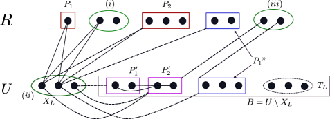
Figure 5: An instance $(G,k)$ of Locating-Dominating Set. Set $U$ is a minimum-size vertex cover of $G$. The dotted edge denotes that a vertex is adjacent with all the vertices in the set. For the sake of brevity, we do not show all the edges. The vertices in green ellipses are part of solution because of $(i)$ being a part of false-twins, $(ii)$ guessed intersection with $U$, and $(iii)$ the requirement of solution to be a dominating set. Note that the vertices $T_{L}$ are not dominated by the partial solution $Y_{L}$. Parts $P_{1},P_{2},P^{\prime}_{1},P^{\prime}_{2},$ and $P^{\prime\prime}_{1}$ are parts of partition of $R\cup B$ induced by $Y_{L}$.

At this stage, $Y_{L}$ dominates all the vertices in $R$. However, it may not dominate all the vertices in $B$. The remaining (to be chosen) vertices in $L$ are part of $R$ and are responsible for dominating the remaining vertices in $B$ and to locate all the vertices in $R\cup B$. See Figure 5 for an illustration. As the remaining solution, i.e., $L\setminus Y_{L}$, does not intersect $B$, it is safe to ignore the edges both whose endpoints are in $B$. The vertices in $Y_{L}$ induce a partition of the vertices of the remaining graph, according to their neighborhood in $Y_{L}$. We can redefine the objective of selecting the remaining vertices in a locating-dominating set as to refine this partition such that each part contains exactly one vertex. Partition refinement is a classic concept in algorithms, see [36]. However in our case, the partition is not standalone, as it is induced by a solution set. To formalize this intuition, we introduce the following notation.

Definition 6.4 (Partition Induced by $C$ and Refinement).

For a subset $C\subseteq V(G)$, define an equivalence relation $\sim_{C}$ on $V\subseteq V(G)\setminus C$ as follows: for any pair $u,v\in V$, $u\sim_{C}v$ if and only if $N(u)\cap C=N(v)\cap C$. The partition of $V$ induced by $C$, denoted by $\mathcal{P}(C)$, is the partition defined as follows:

$$\mathcal{P}(C)=\{U\mid U=\{c\}\text{ for some }c\in C\text{ or }U\text{ is an equivalence class of }\sim_{C}\}.$$

Moreover, for two partitions $\mathcal{P}$ and $\mathcal{Q}$ of $V$, a refinement of $\mathcal{P}$ by $\mathcal{Q}$, denoted by $\mathcal{P}\Cap\mathcal{Q}$, is the partition defined as $\{P\cap Q:P\in\mathcal{P},Q\in\mathcal{Q}\}$.

Suppose $V=V(G)$ and $\mathcal{P}$ and $\mathcal{Q}$ are two partitions of $V(G)$, then $\mathcal{P}\Cap\mathcal{Q}$ is also a partition of $V(G)$. We say a partition $\mathcal{P}$ is the identity partition if every part of $\mathcal{P}$ is a singleton set. With these definitions, we define the following auxiliary problem.

Annotated Red-Blue Partition Refinement Input: A bipartite graph $G$ with bipartition $\langle R,B\rangle$ of $V(G)$; a partition $\mathcal{Q}$ of $R\cup B$; a collection of forced solution vertices $C_{0}\subseteq R$; a collection of vertices $T_{L}\subseteq B$ that needs to be dominated; and an integer $\lambda$. Question: Does there exist a set $C$ of size at most $\lambda$ such that $C_{0}\subseteq C\subseteq R$, $C$ dominates $T_{L}$, and $\mathcal{Q}\Cap\mathcal{P}(C)$ is the identity partition of $R\cup B$?

Suppose there is an algorithm $\mathcal{A}$ that solves Annotated Red-Blue Partition Refinement in time $f(|B|)\cdot(|R|+|B|)^{\mathcal{O}(1)}$. Then, there is an algorithm that solves Locating-Dominating Set in time $2^{\mathcal{O}(\textsf{vc})}\cdot f(\textsf{vc})\cdot n^{\mathcal{O}(1)}$. Consider the algorithm described so far in this subsection. The algorithm then calls $\mathcal{A}$ as a subroutine with the bipartite graph obtained from $G$ by deleting all the vertices in $X_{L}$ and removing all the edges in $B$ with $\langle R,B\rangle$ as bipartition. It sets $\mathcal{Q}$ as the partition of $R\cup B$ induced by $Y_{L}$, $C_{0}=Y_{L}\cap R$, $T_{L}=B\setminus N[Y_{L}]$, and $\lambda=k-|Y_{L}|$. Note that $T_{L}$ is the collection of vertices that are not dominated by the partial solution $Y_{L}$. The correctness of the algorithm follows from the correctness of $\mathcal{A}$ and the fact that for two sets $C_{1},C_{2}\subseteq V(G)$, $C_{1}\cup C_{2}$ is a locating-dominating set of $G$ if and only if $\mathcal{P}(C_{1})\Cap\mathcal{P}(C_{2})$ is the identity partition of $V(G)$. Hence, it suffices to prove the following lemma.

Lemma 6.5.

There is an algorithm that solves Annotated Red-Blue Partition Refinement in time $2^{\mathcal{O}(|B|\log|B|)}\cdot(|R|+|B|)^{\mathcal{O}(1)}$.

The remainder of the subsection is devoted to prove Lemma 6.5. We present the algorithm that can roughly be divided into three parts. In the first part, the algorithm processes the partition $\mathcal{Q}$ of $R\cup B$ with the goal of reaching to a refinement of partition $\mathcal{Q}$ such that every part is completely contained either in $R$ or in $B$. Then, we introduce some terms to obtain a ‘set-cover’ type dynamic programming. We also introduce three conditions that restrict the number of dynamic programming states we need to consider to $2^{\mathcal{O}(|B|\log(|B|))}\cdot|R|$. Finally, we state the dynamic programming procedure, prove its correctness and argue about its running time.

Pre-processing the Partition.

Consider the partition $\mathcal{P}(C_{0})$ of $R\cup B$ induced by $C_{0}$, and define $\mathcal{P}_{0}=\mathcal{Q}\Cap\mathcal{P}(C_{0})$. We classify the parts in $\mathcal{P}_{0}$ into three classes depending on whether they intersect with $R$, $B$, or both. Let $P_{1},P_{2},\ldots,P_{t}$ be an arbitrary but fixed order on the parts of $\mathcal{P}_{0}$ that are completely in $R$. Similarly, let $P^{\prime}_{1},P^{\prime}_{2},\ldots,P^{\prime}_{t^{\prime}}$ be an arbitrary but fixed order on the parts that are completely in $B$. Also, let $P^{\prime\prime}_{1},P^{\prime\prime}_{2},\ldots,P^{\prime\prime}_{t^{\prime\prime}}$ be the collection of parts that intersect $R$ as well as $B$. Formally, we have $P_{j}\subseteq R$ for any $j\in[t]$, $P^{\prime}_{j^{\prime}}\subseteq B$ for any $j^{\prime}\in[t]$, and $P^{\prime\prime}_{j^{\prime\prime}}\cap R\neq\emptyset\neq P^{\prime\prime}_{j^{\prime\prime}}\cap B$ for any $j^{\prime\prime}\in[t]$. See Figure 6 for an illustration.

Figure 6: Instance of the Annotated Red-Blue Partition Refinement problem. Vertices in green ellipse denotes set $C_{0}$ whereas dotted ellipse denote vertices in $T_{L}$, and the partition $\mathcal{Q}=\{P_{1},P_{2},P^{\prime}_{1},P^{\prime}_{2},P^{\prime\prime}_{1}\}$. The vertices in the rectangles denote vertices in $T^{\circ}_{L}$.

Recall that $T_{L}$ is the collection of vertices in $B$ that are required to be dominated. The algorithm first expands this set so that it is precisely the collection of vertices that need to be dominated by the solution $C$. In other words, at present, the required condition is $T_{L}\subseteq N(C)$, whereas, after the expansion, the condition is $T_{L}=N(C)$. Towards this, it first expands $T_{L}$ to include $N(C_{0})$. It then uses the property that the final partition needs to be the identity partition to add some more vertices in $T_{L}$.

Consider parts $P^{\prime}_{j^{\prime}}$ or $P^{\prime\prime}_{j^{\prime\prime}}$ of $\mathcal{P}_{0}$. Suppose that $P^{\prime}_{j^{\prime}}$ (respectively, $P^{\prime\prime}_{j^{\prime\prime}}\cap B$) contains two vertices that are not dominated by the final solution $C$, then these two vertices would not be separated by it and hence would remain in one part, a contradiction. Therefore, any feasible solution $C$ needs to dominate all vertices but one in $P^{\prime}_{j^{\prime}}$ (respectively in $P^{\prime}_{j^{\prime}}\cap B$).

• The algorithm modifies $T_{L}$ to include $N(C_{0})$. Then, it iterates over all the subsets $T^{\circ}_{L}$ of $B\setminus T_{L}$ such that for any $j^{\prime}\in[t^{\prime}]$ and $j^{\prime\prime}\in[t^{\prime\prime}]$, $|P^{\prime}_{j^{\prime}}\cap(T^{\circ}_{L}\cup T_{L})|\leq 1$ and $|(P^{\prime\prime}_{j^{\prime\prime}}\cap B)\cap(T^{\circ}_{L}\cup T_{L})|\leq 1$.

Consider a part $P_{j}$ of $\mathcal{P}_{0}$, which is completely contained in $R$. As $R$ is an independent set and the final solution $C$ is not allowed to include any vertex in $B$, for any part $P_{j}$, there is at most one vertex outside $C$, i.e., $|P_{j}\setminus C|\leq 1$. However, unlike the previous step, the algorithm cannot enumerate all the required subsets of $R$ in the desired time. Nonetheless, it uses this property to safely perform the following sanity checks and modifications.

• Consider parts $P_{j}$ or $P^{\prime\prime}_{j^{\prime\prime}}$ of $\mathcal{P}_{0}$. Suppose there are two vertices in $P_{j}$ (respectively $P^{\prime\prime}_{j^{\prime\prime}}\cap R$) that are adjacent with some vertices in $B\setminus T_{L}$. Then, discard this guess of $T^{\circ}_{L}$ and move to the next subset.

• Consider parts $P_{j}$ or $P^{\prime\prime}_{j^{\prime\prime}}$ of $\mathcal{P}_{0}$. Suppose there is a unique vertex, say $r$, in $P_{j}$ (respectively, in $P^{\prime\prime}_{j^{\prime\prime}}\cap R$) that is adjacent with some vertex in $B\setminus T_{L}$. Then, modify $C_{0}$ to include all the vertices in $P_{j}\setminus\{r\}$ or in $(P^{\prime\prime}_{j^{\prime\prime}}\cup R)\setminus\{r\}$.

Consider a part $P^{\prime\prime}_{j^{\prime\prime}}$ of $\mathcal{P}_{0}$ and suppose $|(P^{\prime\prime}_{j^{\prime\prime}}\cap B)\setminus T_{L}|=0$. Alternately, every vertex in $P^{\prime\prime}_{j^{\prime\prime}}\cap B$ is adjacent to some vertex in the final solution $C$. As $R$ is an independent set and $C\subseteq R$, this domination condition already refines the partition $P^{\prime\prime}_{j^{\prime\prime}}$, i.e. every vertex in $(P^{\prime\prime}_{j^{\prime\prime}}\cap B)$ needs to be adjacent with some vertex in $C$ whereas no vertex in $(P^{\prime\prime}_{j^{\prime\prime}}\cap R)$ can be adjacent with $C$. This justifies the following modification.

• For a part $P^{\prime\prime}_{j^{\prime\prime}}$ of $\mathcal{P}_{0}$ such that $|(P^{\prime\prime}_{j^{\prime\prime}}\cap B)\setminus T_{L}|=0$, the algorithm modifies the input partition $\mathcal{P}_{0}$ by removing $P^{\prime\prime}_{j^{\prime\prime}}$ and adding two new parts $P_{j}:=P^{\prime\prime}_{j^{\prime\prime}}\cap R$ and $P^{\prime}_{j^{\prime}}:=P^{\prime\prime}_{j^{\prime\prime}}\cap B$.

Consider a part $P^{\prime\prime}_{j^{\prime\prime}}$ of $\mathcal{P}_{0}$ and suppose $|(P^{\prime\prime}_{j^{\prime\prime}}\cap B)\setminus T_{L}|=1$. Let $b$ be the unique vertex in $(P^{\prime\prime}_{j^{\prime\prime}}\cap B)\setminus T_{L}$. Suppose there is a (unique) vertex, say $r$, in $(P^{\prime\prime}_{j^{\prime\prime}}\cap R)$ that is not part of the final solution $C$. However, this implies that both $b$ and $r$ are in the same part, a contradiction.

• For part $P^{\prime\prime}_{j^{\prime\prime}}$ of $\mathcal{P}_{0}$ such that $|(P^{\prime\prime}_{j^{\prime\prime}}\cap B)\setminus T_{L}|=1$, the algorithm includes all the vertices $(P^{\prime\prime}_{j^{\prime\prime}}\cap R)$ into $C_{0}$ (which, by definition, modifies $\mathcal{P}_{0})$. Also, it removes $P^{\prime\prime}_{j^{\prime\prime}}$ from $\mathcal{P}_{0}$ and adds $P^{\prime}_{j^{\prime}}:=P^{\prime\prime}_{j^{\prime\prime}}\cap B$.

These modifications ensure that any part of $\mathcal{P}_{0}$ is either completely contained in $R$ or completely contained in $B$.

Setting up the Dynamic Programming.

Define $\ell=|R\setminus C_{0}|$ and suppose $\{r_{1},r_{2},\dots,r_{\ell}\}$ be the reordering of vertices in $R\setminus C_{0}$ such that any part in $P_{j}$ contains the consecutive elements in the order. Formally, for any $i_{1}<i_{2}<i_{3}\in\{1,2,\dots,|R\setminus C_{0}|\}$ and $t^{\circ}\in\{1,2,\dots,t\}$, if $r_{i_{1}}\in P_{t^{\circ}}$ and $r_{i_{3}}\in P_{t^{\circ}}$, then $r_{i_{2}}\in P_{t^{\circ}}$. Define a function $\pi:\{1,2,\dots,|R\setminus C_{0}|\}\mapsto\{1,2,\dots,t\}$ such that $\pi(r_{i})=t^{\circ}$ if and only if vertex $r_{i}$ is in part $P_{t^{\circ}}$.

For the remaining part, the algorithm relies on a ‘set cover’ type dynamic programming. For every integer $i\in[0,\ell]$, define $R_{i}=\{r_{1},r_{2},\dots,r_{i}\}$. Then, in a ‘set cover’-type dynamic programming, tries to find the optimum size of a subset of $R_{i}$ that dominates all the vertices in $S$, which is a subset of $T$. However, two different optimum solutions in $R_{i}$ will induce different partitions of $R\cup B$. To accommodate this, we define the notion of valid tuples. For an integer $i\in[0,\ell]$ and a subset $S\subseteq T$, we say a tuple $(i,\mathcal{P},S)$ is a valid tuple if $\mathcal{P}$ is a refinement of $\mathcal{P}_{0}$ and it satisfies the three properties mentioned below. Note that these properties are the consequences of the fact that we require $\mathcal{P}$ to be such that, for any (partial) solution $C$ with vertices upto $r_{i}$ in the ordering of $R\setminus C_{0}$, we can have $\mathcal{P}(C)=\mathcal{P}$ and $N(C)=S$.

1. For any $i\in[0,\ell]$, the partition $\mathcal{P}$ restricted to any $P_{j}$, where $j\in[\pi(i)-1]$, is the identity partition of $P_{j}$. This is because, if on the contrary, $\mathcal{P}$ restricted to $P_{j}$ for some $j\in[\pi(i)-1]$ is not the identity partition, it would imply that there exists a part $P$, say, of $\mathcal{P}$ with $|P|\geq 2$ which cannot be refined by picking vertices of $R$ in the final solution $C$ (upto $r_{\ell}$), as $R$ is an independent set.

2. There may be at most one vertex $r$, say, in $P_{\pi(i)}\cap R_{i}$ which is not yet picked in $C$. This is because if two vertices $r^{\prime},r^{\prime\prime}$ of $P_{\pi(i)}\cap R_{i}$ are not picked in $C$, the final solution $C$ cannot induce the identity partition, since $\{r^{\prime}\},\{r^{\prime\prime}\}\notin\mathcal{P}(C)$. Thus, since for any $r^{\prime}\in P_{\pi(i)}\cap R_{i}\setminus\{r\}$, we have $\{r^{\prime}\}\in\mathcal{P}(C)$, we therefore require the partition $P$ of $\mathcal{P}$ to be a singleton set if $P\cap P_{\pi(i)}\cap R_{i}\neq\emptyset$ and $r\notin P$. Moreover, since $(\{r\}\cup P_{\pi(i)}\setminus R_{i})\in\mathcal{P}(C)$, we require that for $r\in P$, the part $P$ must be $(\{r\}\cup P_{\pi(i)}\setminus R_{i})\in\mathcal{P}(C)$.

3. Since any (partial) solution upto $r_{i}$ does not refine any of the parts $P_{\pi(i)+1},\ldots,P_{t}$, for every part $P\in\mathcal{P}$ that does not intersect $P_{1}\cup P_{2}\cup\ldots\cup P_{\pi(i)}$, $P$ must be of the form $P_{x}$, where $x\in[\pi(i)+1,t]$.

From the above three properties of how the refinements $\mathcal{P}$ of $\mathcal{P}_{0}$ can be, we find that $\mathcal{P}$ restricted to $B$ can be any partition on $B$ (which can be at most $\mathcal{O}(2^{\mathcal{O}(|B|\log|B|)})$ many) and the sets $P\in\mathcal{P}$ containing the vertex $r\in P_{\pi(i)}$ can be as many as the number of vertices in $P_{\pi(i)}\cap R_{i}$, that is, at most $|R|$ many. Let $\mathcal{X}$ be the collection of all the valid tuples. Then, for any $i\in[\ell]$ and any $S\subseteq T$, the number of partitions $\mathcal{P}$ for which $(i,\mathcal{P},S)\in\mathcal{X}$ is $\mathcal{O}(2^{\mathcal{O}(|B|\log|B|)}\cdot|R|)$.

Dynamic Programming.

For every valid tuple $(i,\mathcal{P},S)\in\mathcal{X}$, we define

$\texttt{opt}[i,\mathcal{P},S]$	=	the minimum cardinality of a set $C$ that is compatible with the
		valid triple $(i,\mathcal{P},S)$, i.e., $(i)\ C\subseteq R_{i}\ (ii)\ \mathcal{P}_{0}\Cap\mathcal{P}(C)=\mathcal{P}\ \&\ (iii)\ N(C)=S$.

If no such $(i,\mathcal{P},S)$-compatible set exists, then we let the value of $\texttt{opt}[i,\mathcal{P},S]$ to be $\infty$. Moreover, any $(i,\mathcal{P},S)$-compatible set $C$ of minimum cardinality is called a minimum $(i,\mathcal{P},S)$-compatible set. The quantities $\texttt{opt}[i,\mathcal{P},S]$ for all $(i,\mathcal{P},S)\in\mathcal{X}$ are updated inductively. Then finally, the quantity $\texttt{opt}[\ell,\mathcal{I}(R\cup B),T]$ gives us the required output of the problem. To start with, we define the quantity $\texttt{opt}[0,\mathcal{P}_{0},N(C_{0})]=|C_{0}|$ and set $\texttt{opt}[i,\mathcal{P},S]=\infty$ for each triple $(i,\mathcal{P},S)\in\mathcal{X}$ such that $(i,\mathcal{P},S)\neq(0,\mathcal{P}_{0},N(C_{0}))$. Then, the value of each $\texttt{opt}[i,\mathcal{P},S]$ updates by the following dynamic programming formula.

$$\texttt{opt}[i,\mathcal{P},S]=\min\begin{cases}\texttt{opt}[i-1,\mathcal{P},S],\\ 1+\min\limits_{\begin{subarray}{c}\mathcal{P}^{\prime}\Cap\mathcal{P}(r_{i})=\mathcal{P},\\ S^{\prime}\cup N(r_{i})=S\end{subarray}}\texttt{opt}[i-1,\mathcal{P}^{\prime},S^{\prime}].\end{cases}$$ (1)

Proof of Correctness.

We prove by induction on $i$ that the above formula is correct. In other words, we show that, for any $i\in[\ell]$, if the values of $\texttt{opt}[j,\mathcal{P}^{\prime},S^{\prime}]$ are correctly calculated for all triples $(j,\mathcal{P}^{\prime},S^{\prime})\in\mathcal{X}$ with $j\in[0,i-1]$, then for any couple $(\mathcal{P},S)$, the above equality holds. Before this, we prove some technical properties.

Claim 1.

Let $(i,\mathcal{P},S)\in\mathcal{X}$. Then, the following hold.

• The triple $(i-1,\mathcal{P},S)\in\mathcal{X}$ as well. Moreover, if $C$ is a $(i-1,\mathcal{P},S)$-compatible set, then $C$ is also a $(i,\mathcal{P},S)$-compatible set. In particular, $\texttt{opt}[i,\mathcal{P},S]\leq\texttt{opt}[i-1,\mathcal{P},S]$.

• Let $(i-1,\mathcal{P}^{\prime},S^{\prime})\in\mathcal{X}$ such that $\mathcal{P}^{\prime}\Cap\mathcal{P}(r_{i})=\mathcal{P}$ and $S^{\prime}\cup N(r_{i})=S$. If $C^{\prime}$ is a $(i-1,\mathcal{P}^{\prime},S^{\prime})$-compatible set, then $C=C^{\prime}\cup\{r_{i}\}$ is a $(i,\mathcal{P},S)$-compatible set. In particular, $\texttt{opt}[i,\mathcal{P},S]\leq 1+\texttt{opt}[i-1,\mathcal{P}^{\prime},S^{\prime}]$.

Proof 6.6.

We first show that $(i-1,\mathcal{P},S)\in\mathcal{X}$. So, let $P\in\mathcal{P}$ be such that $P\cap R_{i-1}\neq\emptyset$ and $|P|\geq 2$. It implies that $P\cap R_{i}\neq\emptyset$ as well and hence, $P\cap P_{j}=\emptyset$ for all $j\in[0,\pi(i)-1]$ and $P\cap P_{\pi(i)}$ is singleton. If $\pi(i-1)<\pi(i)$, then $\pi(i-1)=\pi(i)-1$ and hence, $P\cap P_{j}=\emptyset$ for all $j\in[0,\pi(i-1)]$. In other words, $P\cap R_{i-1}=\emptyset$, a contradiction to our assumption. Therefore, we must have $\pi(i-1)=\pi(i)$ and thus, clearly, $(i-1,\mathcal{P},S)\in\mathcal{X}$. Now, let $C$ is a $(i-1,\mathcal{P},S)$-compatible set. Then clearly $C$ is also a $(i,\mathcal{P},S)$-compatible set. Then, the inequality follows immediately.

Now, we prove the second point. Let $C^{\prime}$ be a $(i-1,\mathcal{P}^{\prime},S^{\prime})$-compatible set. Then, we have the following.

• $C=C^{\prime}\cup\{r_{i}\}\subset R_{i}$;

• $\mathcal{P}_{0}\Cap\mathcal{P}(C)=\mathcal{P}_{0}\Cap\mathcal{P}(C^{\prime})\Cap\mathcal{P}(r_{i})=\mathcal{P}^{\prime}\cap\mathcal{P}(r_{i})=\mathcal{P}$; and

• $N(C)=N(C^{\prime})\cup N(r_{i})=S^{\prime}\cup N(r_{i})=S$.

This implies that the set $C$ is a $(i,\mathcal{P},S)$-compatible set. Now, if $\texttt{opt}[i-1,\mathcal{P}^{\prime},S^{\prime}]=\infty$, then, clearly, $\texttt{opt}[i,\mathcal{P},S]\leq 1+\infty=1+\texttt{opt}[i-1,\mathcal{P},S]$. Lastly, if $\texttt{opt}[i-1,\mathcal{P}^{\prime},S^{\prime}]<\infty$ and $C^{\prime}$ is a minimum $(i-1,\mathcal{P}^{\prime},S^{\prime})$-compatible set, since $C$ is $(i,\mathcal{P},S)$-compatible, we have $\texttt{opt}[i,\mathcal{P},S]\leq|C|=1+|C^{\prime}|=1+\texttt{opt}[i-1,\mathcal{P}^{\prime},S^{\prime}]$.

We now prove by induction on $i$ that Equation (1) is correct. In other words, we show that, for any $i\in[\ell]$, if the values of $\texttt{opt}[j,\mathcal{P}^{\prime},S^{\prime}]$ are correctly calculated for all triples $(j,\mathcal{P}^{\prime},S^{\prime})\in\mathcal{X}$ with $j\in[0,i-1]$, then for any couple $(\mathcal{P},S)$, the above equality holds. Let us therefore assume that, for all triples $(j,\mathcal{P}^{\prime},S^{\prime})$ with $j\in[0,i-1]$, the values of $\texttt{opt}[j,\mathcal{P}^{\prime},S^{\prime}]$ are correctly calculated.

To begin with, we show that if no $(i,\mathcal{P},S)$-compatible set exists, then Equation (1) must compute $\infty$ as the value of $\texttt{opt}[i,\mathcal{P},S]$. In other words, we prove that the value of the RHS in Equation (1) is $\infty$. On the contrary, if $\texttt{opt}[i-1,\mathcal{P},S]<\infty$, then there exists a $(i-1,\mathcal{P},S)$-compatible set $C$ which, by Claim 1(1), is a $(i,\mathcal{P},S)$-compatible set. This contradicts our assumption in this case and therefore, $\texttt{opt}[i-1,\mathcal{P},S]=\infty$. Similarly, if we assume that $\texttt{opt}[i-1,\mathcal{P}^{\prime},S^{\prime}]<\infty$ for some refinement $\mathcal{P}^{\prime}$ of $\mathcal{P}_{0}$ and some subset $S^{\prime}$ of $T$ such that $\mathcal{P}^{\prime}\Cap\mathcal{P}(r_{i})=\mathcal{P}$ and $S^{\prime}\cup N(r_{i})=S$, then there exists a $(i-1,\mathcal{P}^{\prime},S^{\prime})$-compatible set $C^{\prime}$. Therefore, by Claim 1(2), the set $C=C^{\prime}\cup\{r_{i}\}$ a $(i,\mathcal{P},S)$-compatible set. This again implies a contradiction to our assumption in this case and therefore, $\texttt{opt}[i-1,\mathcal{P}^{\prime},S^{\prime}]=\infty$. Hence, this proves that RHS $=\infty$ in Equation (1).

In view of the above argument, therefore, we assume for the rest of the proof that $\texttt{opt}[i,\mathcal{P},S]<\infty$. We then show that LHS $=$ RHS in Equation (1). To begin with, we first show that LHS $\leq$ RHS in Equation (1). This is true since, by Claim 1(1), we have $\texttt{opt}[i,\mathcal{P},S]\leq\texttt{opt}[i-1,\mathcal{P},S]$ and, by Claim 1(2), for any $(i-1,\mathcal{P}^{\prime},S^{\prime})\in\mathcal{X}$ such that $\mathcal{P}^{\prime}\cap\mathcal{P}(r_{i})=\mathcal{P}$ and $S^{\prime}\cup N(r_{i})=S$, we have $\texttt{opt}[i,\mathcal{P},S]\leq 1+\texttt{opt}[i-1,\mathcal{P}^{\prime},S^{\prime}]$.

We now prove the reverse, that is, the inequality LHS $\geq$ RHS in Equation (1). Recall that $\texttt{opt}[i,\mathcal{P},S]<\infty$ and hence, $\texttt{opt}[i,\mathcal{P},S]=|C|$ for some minimum $(i,\mathcal{P},S)$-compatible set $C$. We consider the following two cases.

• Case 1 ($r_{i}\notin C$). In this case, $C$ is a $(i-1,\mathcal{P},S)$-compatible set which implies that RHS $\leq\texttt{opt}[i-1,\mathcal{P},S]\leq|C|=\texttt{opt}[i,\mathcal{P},S]$.

• Case 2 ($r_{i}\in C$). Let $C^{\prime}=C\setminus\{r_{i}\}$. Then, $C^{\prime}$ is a $(i-1,\mathcal{P}^{\prime},S^{\prime})$-compatible set, where $\mathcal{P}^{\prime}\cap\mathcal{P}(r_{i})=\mathcal{P}$ and $S^{\prime}\cup N(r_{i})=S$. Therefore, we have $\texttt{opt}[i-1,\mathcal{P}^{\prime},S^{\prime}]\leq|C^{\prime}|$ which implies that RHS $\leq 1+\texttt{opt}[i-1,\mathcal{P}^{\prime},S^{\prime}]\leq 1+|C^{\prime}|=|C|=\texttt{opt}[i,\mathcal{P},S]$.

This proves that LHS = RHS in Equation (1) and hence the correctness of the algorithm.

Running Time.

As mentioned before, given any $i\in[\ell]$ and any $S\subseteq T$, the number of partitions $\mathcal{P}$ for which $(i,\mathcal{P},S)\in\mathcal{X}$ is $2^{\mathcal{O}(|B|\log|B|)}\cdot|R|$. Moreover, the number of possible subsets $S$ of $T$ is at most $2^{|T|}\in 2^{\mathcal{O}(|B|)}$. Therefore, there are at most $|R|\cdot 2^{\mathcal{O}(|B|\log|B|)}\cdot|R|\cdot 2^{\mathcal{O}(|B|)}\in 2^{\mathcal{O}(|B|\log|B|)}\cdot|R|^{\mathcal{O}(1)}$ many states of the dynamic programming that need to be calculated. Moreover, to calculate each such $\texttt{opt}[i,\mathcal{P},S]$, another $2^{\mathcal{O}(|B|\log|B|)}\cdot|R|^{\mathcal{O}(1)}$ number of $\texttt{opt}[i-1,\mathcal{P}^{\prime},S]$’s are invoked according to the dynamic programming formula (1). As a result therefore, we obtain a total runtime of $2^{\mathcal{O}(|B|\log|B|)}\cdot|R|^{\mathcal{O}(1)}\times 2^{\mathcal{O}(|B|\log|B|)}\cdot|R|^{\mathcal{O}(1)}$.

This completes the proof of Lemma 6.5.

Beyond vertex cover.

The technique designed in this subsection can in fact be used to obtain algorithms for two related parameters. The distance to clique of a graph is the size of a smallest set of vertices that need to be removed from a graph so that the remaining vertices form a clique. It is a dense analogue of the vertex cover number (which can be seen as the “distance to independent set”). The twin-cover number of a graph [32] is the size of a smallest set of vertices such that the remaining vertices is a collection of disjoint cliques, each of them forming a set of mutual twins. The twin-cover number is at most the vertex cover number, since the vertices not in the vertex cover form cliques of size 1 in the remaining graph.

We can obtain running in time $2^{\mathcal{O}(\textsf{dc}\log\textsf{dc})}\cdot n^{\mathcal{O}(1)}$ and $2^{\mathcal{O}(\textsf{tc}\log\textsf{tc})}\cdot n^{\mathcal{O}(1)}$ , where dc is the distance to clique of the input graph, and tc is the twin-cover cover number of the input graph. In both cases, the arguments are essentially the same as for vc.

For the twin-cover parameterization, let $U$ be a set of vertices of size tc whose removal leaves a collection $\mathcal{C}$ of cliques, each forming a twin-class. Observe that, since we have applied Reduction Rule 6.1 exhaustively, in fact every clique in $\mathcal{C}$ has size at most 2. Moreover, recall that for any two vertices in a twin-class $S$, we need to select any one of them in any solution, thus those vertices are put in $C_{0}$. Note that each such selected vertex dominates its twin in $R$, which thus is the only vertex of $R$ in its part of $\mathcal{Q}$. Apart from this, nothing changes, and we can apply Lemma 6.5 as above.

For distance to clique, $U$ is the set of vertices of size dc whose removal leaves a clique, $R$. Since $R$ forms a clique, we do no longer immediately obtain a bipartite graph, and thus we need a “split graph” version of Lemma 6.5, where $R$ is a clique and $B$ remains an independent set. Here, there are some slight changes during the phase of pre-processing the partition in the proof of Lemma 6.5, since any vertex in $C$ from $R$ dominates the whole of $R$ and can thus potentially locate some vertex of $R$ from some vertex of $B$. Nevertheless, after the pre-processing, as in Lemma 6.5, we obtain a partition where every part is completely included either in $R$ or in $B$. Then, selecting a vertex of $R$ does not distinguish any two other vertices of $R$, and hence the algorithm is exactly the same from that point onwards.

6.2 A Linear Kernel Parameterized by Neighbourhood Diversity

We now show that Locating-Dominating Set admits a linear kernel when parameterized by the neighbourhood diversity of the input graph. Recall that the neighbourhood diversity of a graph $G$ is the smallest integer $d$ such that $G$ can be partitioned into $d$ sets of mutual twin vertices, each set being either a clique or an independent set. It was introduced in [45] and can be computed in linear time $O(n+m)$ using modular decomposition [18]. We show the following, which implies Theorem 1.5(ii).

Lemma 6.7.

Locating-Dominating Set admits a kernelization algorithm that, given an instance $(G,k)$ with $nd(G)=d$, computes an equivalent instance $(G^{\prime},k^{\prime})$ with $2d$ vertices, and that runs in time $\mathcal{O}(nm)$.

Proof 6.8.

We repeatedely apply Reduction Rule 6.1 until there are no sets of mutual twins of size more than 2 in the graph. As each application takes time $\mathcal{O}(n+m)$ (Lemma 6.2), overall this take at most time $\mathcal{O}(n(n+m))=\mathcal{O}(nm)$. Thus, after applying the rule, there are at most two vertices in each neighbourhood equivalence class. Since there are at most $d$ such classes, the resulting graph has at most $2d$ vertices. By Lemma 6.2, this produces an equivalent instance $(G^{\prime},k^{\prime})$.

Corollary 6.9.

Locating-Dominating Set admits an algorithm running in time $2^{\mathcal{O}(d)}+\mathcal{O}(nm)$, where $d$ is the neighbourhood diversity of the input graph.

Proof 6.10.

We first compute in time $\mathcal{O}(nm)$ the linear kernel from Theorem 6.7, that is a graph with $n^{\prime}\leq 2d$ vertices. Then, a simple brute-force algorithm running in time $2^{\mathcal{O}(n^{\prime})}=2^{\mathcal{O}(d)}$ completes the proof.

6.3 A Linear Kernel Parameterized by Feedback Edge Set

A set of edges $X$ of a graph is a feedback edge set if $G-X$ is a forest. The minimum size of a feedback edge set is known as the feedback edge set number (also known as the cyclomatic number) and is denoted by fes. It is well-known that [25] if a graph $G$ has $n$ vertices, $m$ edges, and $r$ components, then ${\textsf{fes}}(G)=m-n+r$.

In this section, we show the following lemma proving Theorem 1.5(iii).

Lemma 6.11.

Locating-Dominating Set admits a kernelization algorithm that, given an instance $(G,k)$ where $G$ has $n$ vertices, $m$ edges and feedback edge set number fes, computes an equivalent instance $(G^{\prime},k^{\prime})$ with $\mathcal{O}(\textsf{fes})$ vertices and edges, and that runs in $\mathcal{O}(mn)$ time.

Note that the proof of Lemma 6.11 is nonconstructive, in the sense that it shows the existence of a large (but constant) number of gadget types with which the kernel can be constructed, however, as there are far too many gadgets, we do not describe them individually.

To describe the kernelization algorithm, we first need to describe graphs of given feedback edge set number. A graph $G$ with $n$ vertices, feedback edge set number fes, and $c$ connected components, has exactly $n+\textsf{fes}-c$ edges. The following is a classic description of such graphs.

Proposition 6.12 ([41, Observation 8]).

Any graph $G$ with feedback edge set number fes is obtained from a multigraph $\widetilde{G}$ with at most $2\textsf{fes}-2$ vertices and $3\textsf{fes}-3$ edges by first subdividing edges of $\widetilde{G}$ arbitrary number of times, and then, repeatedely attaching degree 1 vertices to the graph, and $\widetilde{G}$ can be computed from $G$ in $\mathcal{O}(n+\textsf{fes})$ time.

By Proposition 6.12, we compute the multigraph $\widetilde{G}$ in $\mathcal{O}(n+\textsf{fes})$ time, and we let $\widetilde{V}$ be the set of vertices of $\widetilde{G}$. For every edge $v_{1}v_{2}$ of $\widetilde{G}$, we have either:

1. $v_{1}v_{2}$ corresponds to an edge in the original graph $G$, if $v_{1}v_{2}$ has not been subdivided when obtaining $G$ from $\widetilde{G}$ (then $v_{1}\neq v_{2}$ since $G$ is loop-free), or

2. $v_{1}v_{2}$ corresponds to a component $C$ of the original graph $G$ with $\{v_{1},v_{2}\}$ removed. Moreover, $C$ induces a tree, with two (not necessarily distinct) vertices $c_{1},c_{2}$ in $C$, where $c_{1}$ is the only vertex of $C$ adjacent to $v_{1}$ and $c_{2}$ is the only vertex of $C$ adjacent to $v_{2}$ in $G$. (Possibly, $v_{1}=v_{2}$ and the edge $v_{1}v_{2}$ is a loop of $\widetilde{G}$.)

To avoid dealing with the case of loops, for every component $C$ of $G\setminus\{v_{1}\}$ with a loop at $v_{1}$ in $\widetilde{G}$ and with $c_{1},c_{2}$ defined as above, we select an arbitrary vertex $x$ of the unique path between $c_{1}$ and $c_{2}$ in $G[C]$ and add $x$ to $\widetilde{V}$. As there can be at most fes such loops in $\widetilde{G}$, we can assume that $\widetilde{G}$ is a multigraph with at most $3\textsf{fes}-2$ vertices and $4\textsf{fes}-3$ edges, and no loops.

We may assume that the multigraph $\widetilde{G}$ computed in Proposition 6.12 has at most $3\textsf{fes}-2$ vertices and $4\textsf{fes}-3$ edges, and no loops.

The kernelization algorithm can be described in two steps. First, we need to handle hanging trees, that is, parts of the graph that induce trees and are connected to the rest of the graph via a single edge. Those correspond to the iterated addition of degree 1 vertices to the graph from $\widetilde{G}$ described in Proposition 6.12.

The second step will be to deal with the subgraphs that correspond to the edges of $\widetilde{G}$ as described above.

6.3.1 Handling hanging trees

It is known that there is a linear-time dynamic programming algorithm to solve Locating-Dominating Set on trees [54] (see also [3] for a more general algorithm for block graphs, that also solves several types of problems related to Locating-Dominating Set). To perform such a dynamic programming, one can in fact define the following five types of (partial) solutions. For a tree $T$ rooted at a vertex $v$, we define five types for a subset $L$ of $V(T)$ as follows:

• Type $A$: $L$ dominates all vertices of $V(T)\setminus\{v\}$ and any two vertices of $V(T)\setminus(L\cup\{v\})$ are located.

• Type $B$: $L$ is a dominating set of $T$ and any two vertices of $V(T)\setminus(L\cup\{v\})$ are located;

• Type $C$: $L$ is a locating-dominating set of $T$;

• Type $D$: $L$ is a locating-dominating set of $T$ with $v\in L$;

• Type $E$: $L$ is a locating-dominating set of $T$ such that $v\in L$ and there is no vertex $w$ of $T$ with $N(w)\cap L=\{v\}$;

Next, for convenience, we consider the lexicographic ordering $A<B<C<D<E$. Note that these five types of solution are increasingly constrained (so, if $X<X^{\prime}$, if $L$ is a solution of type $X^{\prime}$, it is also one of type $X$). Those are the five possible behaviours of a locating-dominating set of a supergraph $G$ of $T$, in which $v$ forms a cut-vertex of $G$.

For a tree $T$ rooted at $v$ and $X\in\{A,B,C,D,E\}$, we denote by $opt_{X}(T,v)$ the minimum size of a set $L\subseteq V(T)$ of type $X$. Note that $opt_{C}(T,v)$ is equal to the location-domination number of $T$.

Proposition 6.13.

There is a linear-time dynamic programming algorithm that, for any tree $T$ and root $v$, conjointly computes $opt_{X}(T,v)$ for all $X\in\{A,B,C,D,E\}$.

Proof 6.14.

Use the same ideas as in the dynamic programming algorithms from [3, 54].

We next show that, for a given tree, the optimal values of solutions of different types vary by at most one.

Lemma 6.15.

Let $T$ be a tree with vertex $v$, and let $X,X^{\prime}\in\{A,B,C,D,E\}$ with $X<X^{\prime}$. We have $opt_{X^{\prime}}(T,v)\leq opt_{X}(T,v)\leq opt_{X^{\prime}}(T,v)+1$.

Proof 6.16.

The first inequality follows immediately by noticing that the conditions for types $A$ to $E$ are increasingly constrained. Moreover, all types are feasible by considering $L=V(T)$, so $opt_{X}(T,v)$ is always well-defined. This implies that the first inequality is true.

For the second inequality, assume we have $X^{\prime}\in\{A,B\}$ and $L$ is an optimal solution of type $X^{\prime}$. Then, $L\cup\{v\}$ is a solution of type $E$. If $X^{\prime}\in\{C,D\}$, let $L$ be an optimal solution of type $X^{\prime}$. If $v\notin L$ (then $X^{\prime}=C$), then again $L\cup\{v\}$ is a solution of type $E$. If $v\in L$, possibly some (unique) vertex $w$ of $T$ satisfies $N(w)\cap L=\{v\}$. Then, $L\cup\{w\}$ is a solution of type $E$. Thus, $opt_{X}(T,v)\leq opt_{E}(T,v)\leq opt_{X^{\prime}}(T,v)+1$. In all cases, we have $opt_{X}(T,v)\leq opt_{E}(T,v)\leq opt_{X^{\prime}}(T,v)+1$, as claimed.

By Lemma 6.15, for any rooted tree $(T,v)$, the five values $opt_{X}(T,v)$ (for $X\in\{A,B,C,D,E\}$) differ by at most one, and we know that they increase along with $X$: $opt_{A}(T,v)\leq opt_{B}(T,v)\leq\ldots\leq opt_{E}(T,v)$. Hence, for any rooted tree $(T,v)$, there is one value $X\in\{A,B,C,D,E\}$ where the “shift” occurs. More precisely, whenever $X^{\prime}\leq X$, we have $opt_{X^{\prime}}(T,v)=opt_{X}(T,v)$, and whenever $X^{\prime}>X$, we have $opt_{X^{\prime}}(T,v)=opt_{X}(T,v)+1$. Thus, we can introduce the following definition, which partitions the set of rooted trees according to one of five such possible behaviours.

Definition 6.17 (Rooted tree classes).

For $X\in\{A,B,C,D,E\}$, we define the class $\mathcal{T}_{X}$ as the set of pairs $(T,v)$ such that $T$ is a tree with root $v$, and there is an integer $k$ with $opt_{X^{\prime}}(T,v)=k$ whenever $X^{\prime}\leq X$, and $opt_{X^{\prime}}(T,v)=k+1$ whenever $X^{\prime}>X$ (note that $k$ may differ across the trees in $\mathcal{T}_{X}$).

Note that for the trees in $\mathcal{T}_{E}$, all five types of optimal solutions have the same size.

It is clear by Lemma 6.15 that the set of all possible pairs $(T,v)$ where $T$ is a tree and $v$ a vertex of $T$, can be partitioned into the five classes $\mathcal{T}_{X}$, where $X\in\{A,B,C,D,E\}$. Moreover, it is not difficult to construct small rooted trees for each of these five classes. We next provide five such small rooted trees, each in a different class.

	$T_{A}$	$T_{B}$	$T_{C}$	$T_{D}$	$T_{E}$
$opt_{A}$	0	1	2	1	3
$opt_{B}$	1	1	2	1	3
$opt_{C}$	1	2	2	1	3
$opt_{D}$	1	2	3	1	3
$opt_{E}$	1	2	3	2	3

Table 2: The five rooted tree gadgets with their values of the five $opt_{X}$ functions.

Definition 6.18 (Rooted tree gadgets).

For $X\in\{A,B,C,D,E\}$, let $(T_{X},v_{X})$ be the rooted tree of class $\mathcal{T}_{X}$ from Table 2, and let $k_{X}=opt_{X}(T_{X},v_{X})$.

As these are very small, it is easy to check that the gadgets are indeed in the claimed class.

For $X\in\{A,B,C,D,E\}$, $(T_{X},v_{X})$ belongs to the class $\mathcal{T}_{X}$.

We are now ready to present our first reduction rule.

Reduction Rule 6.19.

Let $(G,k)$ be an instance of Locating-Dominating Set such that $G$ can be obtained from a graph $G^{\prime}$ and a tree $T$, by identifying a vertex $v$ of $T$ with a vertex $w$ of $G^{\prime}$, such that $(T,v)$ is in class $\mathcal{T}_{X}$ with $X\in\{A,B,C,D,E\}$, and with $opt_{X}(T,v)=t$. Then, we remove all vertices of $T\setminus\{v\}$ from $G$ (this results in $G^{\prime}$), we consider $G$ and a copy of the rooted tree gadget $(T_{X},v_{X})$, and we identify $v_{X}$ with $v$, to obtain $G^{\prime\prime}$. The reduced instance is $(G^{\prime\prime},k-t+k_{X})$.

Lemma 6.20.

For an instance $(G,k)$ of Locating-Dominating Set, Reduction Rule 6.19 can be applied exhaustively in time $\mathcal{O}(n^{2})$, and for each application, $(G,k)$ is a YES-instance of Locating-Dominating Set if and only if $(G^{\prime\prime},k-t+k_{X})$ is a YES-instance of Locating-Dominating Set.

Proof 6.21.

To apply Reduction Rule 6.19, one can find all vertices of degree 1 in $G$, mark them, and iteratively mark degree 1 vertices in the subgraph induced by unmarked vertices. Note that a connected subset $S$ of marked vertices induces a tree with a single vertex $v_{S}$ adjacent to a non-marked vertex $w$. Moreover, at the end of the marking process, the subgraph induced by non-marked vertices has minimum degree 2. This process can be done in $\mathcal{O}(n^{2})$ time.

We form the set of candidate trees $T$ by taking the union $S_{w}$ of all marked subsets that are connected to some common unmarked vertex $w$, together with $w$. Note that all these candidate trees are vertex-disjoint. Again, this can be done in $\mathcal{O}(n^{2})$ time. Let $(T,v)$ be such a rooted tree, and let $G^{\prime}$ be the subgraph induced by $V(G)\setminus S_{v}$. Then, we apply the linear-time dynamic programming algorithm of Proposition 6.13 to $(T,v)$ to determine the class $\mathcal{T}_{X}$ to which $(T,v)$ belongs to, for some $X\in\{A,B,C,D,E\}$, as well as $opt_{X}(T,v)=t$ for each $X\in\{A,B,C,D,E\}$. Constructing $(G^{\prime\prime},k-t+k_{X})$ by replacing $T$ by $T_{X}$ in $G$ can then be done in time $\mathcal{O}(|V(T)|)$. Thus, overall applying the reduction rule to all trees takes $\mathcal{O}(n^{2})$ time.

Now, we prove the second part of the statement. Assume we have applied Reduction Rule 6.19 to a single tree $(T,v)$ to $G$,that $(G,k)$ is a YES-instance of Locating-Dominating Set, and let $L$ be an optimal locating-dominating set of $G$ of size at most $k$. Assume that $L\cap V(T)$ is of type $X^{\prime}$ for $X^{\prime}\in\{A,B,C,D,E\}$ with respect to $(T,v)$. Notice that the only interactions between the vertices in $V(T)$ and $V(G^{\prime})$ are through the cut-vertex $v$. If $X^{\prime}\leq X$, then, as $L$ is optimal, we have $|L\cap V(T)|=t$; if $X^{\prime}>X$, then by Lemma 6.15, we have $|L\cap V(T)|=t+1$. Now, we obtain a solution of $G^{\prime\prime}$ from $L^{\prime}=L\cap V(G^{\prime})$ by adding an optimal solution $S_{X^{\prime}}$ of type $X^{\prime}$ of $(T_{X},v_{X})$ to $L^{\prime}$. This has size $k_{X}$ if $X^{\prime}\leq X$ and $k_{X}+1$ if $X^{\prime}>X$. As $S_{X^{\prime}}$ behaves the same as $L\cap V(T)$ with respect to $L^{\prime}$, $L$ is a valid locating-dominating set of $G^{\prime\prime}$. Its size is either $|L|-(t+1)+k_{X}+1$ if $X^{\prime}>X$, or $|L|-t+k_{X}$ if $X\leq X^{\prime}$, which in both cases is at most $k-t+k_{X}$, thus $(G^{\prime\prime},k-t+k_{X})$ is a YES-instance.

The proof of the converse follows by the same argument: essentially, the trees $(T,v)$ and $(T_{X},v_{X})$ are interchangeable.

We now use Lemma 6.20 to apply Reduction Rule 6.19 exhaustively in time $\mathcal{O}(n^{2})$, before proceeding to the second part of the algorithm.

6.3.2 Handling the subgraphs corresponding to edges of $\widetilde{G}$.

To describe the second step of our kernelization algorithm, our aim is to construct tree gadgets similar to those defined above, but with two distinguished vertices. We thus extend the above terminology to this setting. Let $(T,v_{1},v_{2})$, be a tree $T$ with two distinguished vertices $v_{1},v_{2}$. We define types of trees as in the previous subsection. To do so, we first define the types for each of $v_{1}$ and $v_{2}$, and then we combine them. For $X\in\{A,B,C,D,E\}$, a subset $L$ of $V(T)$ is of type $(X,-)$ with respect to $v_{1}$ if:

• Type $(A,-)$: $L$ dominates all vertices of $V(T)\setminus\{v_{1},v_{2}\}$ and any two vertices of $V(T)\setminus(L\cup\{v_{1},v_{2}\})$ are located.

• Type $(B,-)$: $L$ dominates all vertices of $V(T)\setminus\{v_{2}\}$ and any two vertices of $V(T)\setminus(L\cup\{v_{1},v_{2}\})$ are located;

• Type $(C,-)$: $L$ dominates all vertices of $V(T)\setminus\{v_{2}\}$ and any two vertices of $V(T)\setminus(L\cup\{v_{2}\})$ are located;

• Type $(D,-)$: $L$ dominates all vertices of $V(T)\setminus\{v_{2}\}$, $v_{1}\in L$, and any two vertices of $V(T)\setminus(L\cup\{v_{2}\})$ are located;

• Type $(E,-)$: $L$ dominates all vertices of $V(T)\setminus\{v_{2}\}$, $v_{1}\in L$, any two vertices of $V(T)\setminus(L\cup\{v_{2}\})$ are located, and there is no vertex $w$ of $V(T)\setminus\{v_{2}\}$ with $N(w)\cap L=\{v_{1}\}$;

Thus, the idea for a set $L$ of type $(X,-)$ with respect to $v_{1}$ is that there are specific constraints for $v_{1}$, but no constraint for $v_{2}$ (and the usual domination and location constraints for the other vertices). We say that $L$ if of type $(X,Y)$ with respect to $(T,v_{1},v_{2})$ if $L$ is of type $(X,-)$ with respect to $v_{1}$ and of type $(Y,-)$ with respect to $v_{2}$. Thus, we have a total of 25 such possible types.

We let $opt_{X,Y}(T,v_{1},v_{2})$ be the smallest size of a subset $L$ of $T$ of type $(X,Y)$. Next, we argue that one can efficiently compute these values.

Proposition 6.22.

There is a linear-time dynamic programming algorithm that, for any tree $T$ and two vertices $v_{1},v_{2}$, conjointly computes $opt_{X,Y}(T,v_{1},v_{2})$ for all $X,Y\in\{A,B,C,D,E\}$.

Proof 6.23.

The dynamic programming is similar to that of Proposition 6.13. We root $T$ at $v_{1}$. The main difference is that extra care must be taken around $v_{2}$ to only keep the solutions of type $(-,Y)$ for the subtrees that contain $v_{2}$.

Next, similarly to Lemma 6.15, we show that for a triple $(T,v_{1},v_{2})$, the optimal solution values for different types, may vary by at most 2.

Lemma 6.24.

Let $T$ be a tree with vertices $v_{1},v_{2}$ of $T$, and let $X,X^{\prime},Y,Y^{\prime}\in\{A,B,C,D,E\}$ with $X\leq X^{\prime}$ and $Y\leq Y^{\prime}$. If $X=X^{\prime}$ and $Y<Y^{\prime}$ or $X<X^{\prime}$ and $Y=Y^{\prime}$, we have $opt_{X,Y}(T,v_{1},v_{2})\leq opt_{X^{\prime},Y^{\prime}}(T,v_{1},v_{2})\leq opt_{X,Y}(T,v_{1},v_{2})+1$. If $X<X^{\prime}$ and $Y<Y^{\prime}$, we have $opt_{X,Y}(T,v_{1},v_{2})\leq opt_{X^{\prime},Y^{\prime}}(T,v_{1},v_{2})\leq opt_{X,Y}(T,v_{1},v_{2})+2$.

Proof 6.25.

The proof is similar to that of Lemma 6.15. As before, the lower bound is clear since the conditions for type $(X^{\prime},Y^{\prime})$ are more constrained that those for $(X,Y)$. For the upper bound, assume first that $X=X^{\prime}$ or $Y=Y^{\prime}$ (without loss of generality, $Y=Y^{\prime}$). Then, as before, given a solution $S$ of type $(X,Y)$, we can add to $S$ a single vertex in the closed neighbourhood of $v_{1}$ to obtain a solution of type $(E,Y)$. Similarly, if both $X<X^{\prime}$ and $Y<Y^{\prime}$, we can add to $S$ a vertex to the closed neighbourhoods of each of $v_{1}$ and $v_{2}$ and obtain a solution of type $(E,E)$.

By Lemma 6.24, we can introduce the following definition. Note that for a triple $(T,v_{1},v_{2})$, the minimum value of $opt_{X,Y}(T,v_{1},v_{2})$ over all $X,Y\in\{A,B,C,D,E\}$ is reached for $X=Y=A$ (and the maximum, for $X=Y=E$).

Definition 6.26 (Doubly rooted tree classes).

For a function $g:\{A,B,C,D,E\}^{2}\to\{0,1,2\}$, we define the class $\mathcal{T}_{g}$ as the set of triples $(T,v_{1},v_{2})$ such that $T$ is a tree, $v_{1},v_{2}$ are two of its vertices, and for every $(X,Y)\in\mathcal{\{}A,B,C,D,E\}^{2}$, we have $opt_{X,Y}(T,v_{1},v_{2})-opt_{A,A}(T,v_{1},v_{2})=g(X,Y)$.

Note that there are at most $3^{25}$ such classes of triples, since that is the number of possible functions $g$. By Lemma 6.24, these classes define a partition of all sets of triples $(T,v_{1},v_{2})$.

We next define suitable tree gadgets for the above classes of triples. As there is a very large number of possible types of triples, we cannot give a concrete definition of such a gadget, but rather, an existential one.

Definition 6.27 (Doubly-rooted tree gadgets).

For a function $g:\{A,B,C,D,E\}^{2}\to\{0,1,2\}$, let $(T_{g},v_{X},v_{Y})$ be the smallest tree in $\mathcal{T}_{g}$ (if such a tree exists), and let $k_{g}=opt_{A,A}(T_{g},v_{X},v_{Y})$.

We are now ready to present our second reduction rule, which replaces certain triples $(T,v_{1},v_{2})$ by gadgets from Definition 6.27.

Reduction Rule 6.28.

Let $(G,k)$ be an instance of Locating-Dominating Set, with:

• an induced subgraph $G^{\prime}$ of $G$ with two vertices $w_{1},w_{2}$;

• a tree $T$ with two vertices $v_{1},v_{2}$ with $(T,v_{1},v_{2})$ in class $\mathcal{T}_{g}$ with $g:\{A,B,C,D,E\}^{2}\to\{0,1,2\}$, and with $opt_{A,A}(T,v_{1},v_{2})=t$;

• $w_{1},w_{2}$ do not belong to a hanging tree of $G$;

• $G$ can be obtained by taking a copy of $T$ and a copy of $G^{\prime}$ and identifying, respectively, $v_{1}$ with $w_{1}$, and $v_{2}$ with $w_{2}$.

Then, we remove all vertices of $T\setminus\{v_{1},v_{2}\}$ from $G$ (that is, we compute $G^{\prime}$), we consider $G^{\prime}$ and a copy of doubly-rooted tree gadget $(T_{g},v_{X},v_{Y})$, and we identify $v_{X}$ with $v_{1}$ and $v_{Y}$ with $v_{2}$, to obtain $G^{\prime\prime}$. The reduced instance is $(G^{\prime\prime},k-t+k_{g})$.

Lemma 6.29.

For an instance $(G,k)$ of Locating-Dominating Set, Reduction Rule 6.28 can be applied to every tree component corresponding to an edge of $\widetilde{G}$ in time $\mathcal{O}(n\textsf{fes})$, and $(G,k)$ is a YES-instance of Locating-Dominating Set if and only if $(G^{\prime\prime},k-t+k_{g})$ is a YES-instance of Locating-Dominating Set.

Proof 6.30.

To apply the reduction rule as stated, we compute the multigraph $\widetilde{G}$ in time $\mathcal{O}(n+\textsf{fes})$ using Proposition 6.12; by Observation 6.3, we can assume it has no loops and at most $4\textsf{fes}-3$ edges. Now, for every edge $xy$ of $\widetilde{G}$, we select the neighbour $v_{1}$ of $x$ and the neighbour $v_{2}$ of $y$ in $G$, that lie on the $xy$-path corresponding to the edge $xy$ of $\widetilde{G}$. The tree $(T,v_{1},v_{2})$ is the subgraph of $G$ corresponding to the edge $xy$ of $\widetilde{G}$, and $G^{\prime}$ is the subgraph of $G$ obtained by removing $T\setminus\{v_{1},v_{2}\}$ from $G$. Computing all these subgraphs can be done in time $\mathcal{O}(n\textsf{fes})$. Computing the type $\mathcal{T}_{g}$ of $(T,v_{1},v_{2})$ can be done in time $\mathcal{O}(|T|)$ by Proposition 6.22, so overall, the running time of this step is $\mathcal{O}(n\textsf{fes})$.

Note that all the computed subgraphs are vertex-disjoint, we can thus now apply Reduction Rule 6.28 in time $\mathcal{O}(|T|)$ to each tree $T$, noting that the gadget $T_{g}$ is of constant size.

For the second part of the statement, the arguments are the same as those of Lemma 6.20: since they belong to the same class $\mathcal{T}_{g}$, the trees $(T,v_{1},v_{2})$ and $(T_{g},v_{X},v_{Y})$ have the same behaviour with respect to Locating-Dominating Set and the overall solution for the graph.

6.3.3 Completion of the proof

By Lemma 6.20 and Lemma 6.29, we have applied Reduction Rule 6.19 and Reduction Rule 6.28 in time $\mathcal{O}(n^{2}+n\textsf{fes})=\mathcal{O}(mn)$. As we have started from a graph $\widetilde{G}$ with at most $3\textsf{fes}-2$ vertices and $4\textsf{fes}-3$ edges, and replaced each vertex of $\widetilde{G}$ by one constant-size tree-gadget from Definition 6.18 and each edge of $\widetilde{G}$ by one constant-size doubly-rooted tree gadget from Definition 6.27, the resulting graph has $\mathcal{O}(\textsf{fes})$ vertices and edges, as claimed.

The algorithm running in time $2^{\mathcal{O}(\textsf{fes})}+n^{\mathcal{O}(1)}$ follows by first computing the kernel and then solving Locating-Dominating Set in time $2^{\mathcal{O}(n)}=2^{\mathcal{O}(\textsf{fes})}$ on that kernel. This completes the proof of Lemma 6.11.

7 Modifications for Test Cover

In this section, we present the small (but crucial) modifications required to obtain similar results as mentioned in previous section for Test Cover. As in this problem, one only need to ‘locate’ elements, the reductions in this case are often simpler than the corresponding reductions for Locating-Dominating Set to prove a conditional lower bound. We restate the problem definition for readers’ convenience.

Test Cover Input: A set of items $U$, a collection of subsets of $U$ called tests and denoted by $\mathcal{F}$, and an integer $k$. Question: Does there exist a collection of at most $k$ tests such that for each pair of items, there is a test that contains exactly one of the two items? Auxiliary Graph: A bipartite graph $G$ on $n$ vertices with bipartition $\langle R,B\rangle$ of $V(G)$ such that sets $R$ and $B$ contain a vertex for every set in $\mathcal{F}$ and for every item in $U$, respectively, and $r\in R$ and $b\in B$ are adjacent if and only if the set corresponding to $r$ contains the element corresponding to $b$.

We note that description of the auxiliary bipartite graph $G$ is sufficient to describe the instance of Test Cover. We find it notationally cleaner to work with encoding of the instance.

7.1 Incompressibility of Test Cover

In this section, we prove Thereom 1.1 for Test Cover. Our reduction is a modification (and also a simplification) of the reduction mentioned in Section 3. We transfer the incompressibility of Red-Blue Dominating Set to Test Cover. Once again, it is safe to assume that $G^{\prime}$ does not contain an isolated vertex, $R^{\prime}\leq 2^{|B^{\prime}|}$, and $k^{\prime}\leq|B^{\prime}|$.

Reduction

For notational convenience, instead of specify an instance of Test Cover, we specify the auxiliary graph as mentioned in the definition. The reduction takes as input an instance $(G^{\prime},\langle R^{\prime},B^{\prime}\rangle,k^{\prime})$ of Red-Blue Dominating Set and constructs an instance $(G,\langle R,B\rangle,k)$ of Test Cover. Suppose we have $R^{\prime}=\{r^{\prime}_{1},r^{\prime}_{2},\dots,r^{\prime}_{|R|}\}$ and $B^{\prime}=\{b^{\prime}_{1},b^{\prime}_{2},\dots,b^{\prime}_{|B|}\}$. The reduction constructs graph $G$ in the following steps. See Figure 2 for an illustration.

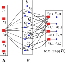
Figure 7: An illustrative example of the graph constructed by the reduction. Red (squared) nodes denote the tests whereas blue (filled circle) nodes the elements. The adjacency across $B$ and $\texttt{bit-rep}(B)$ is same as it was mentioned in Section 3. For brevity, we only show the edges incident on $r_{3}$. The dotted line represents a non-edge. In this example, test corresponding to $r_{3}$ only contains element corresponding to $b_{2}$. It is easy to see that $r_{3}$ can only distinguish between the pair $(b^{\circ}_{2},b^{\star}_{2})$.

• It adds sets of vertices $R$ and $B$ to $G$, where $R$ contains a vertex corresponding to each vertex in $R^{\prime}$ and $B$ contains two vertices corresponding to each vertex in $B^{\prime}$. Formally, $R=\{r_{i}|\ i\in[|R^{\prime}|]\}$ and $B=\{b^{\circ}_{i},b^{\star}_{i}|\ i\in[|B^{\prime}|]\}$.

• The reduction adds a bit representation gadget to locate set $B$. It adds vertices such that for any pair $b^{\circ}_{j},b^{\star}_{j}$, the supplementary vertices adjacent to them are identical.

  • The reduction sets $p:=\lceil\log(|B|/2)\rceil+1$ and for every $i\in[p]$, it adds two vertices $z_{i,1}$ and $z_{i,2}$ and edge $(z_{i,1},z_{i,2})$. It adds all $z_{i,1}$’s to $R$ and all $z_{i,2}$’s to $B$.

  • For every integer $j\in[|B|/2]$, let $\texttt{bit}(j)$ denote the binary representation of $j$ using $q$ bits. Connect $b^{\circ}_{j},b^{\star}_{j}\in B$ with $z_{i,1}$ if the $i^{th}$ bit (going from left to right) in $\texttt{bit}(j)$ is $1$.

  • It add two vertices $z_{0,1}$ and $z_{0,2}$, and edge $(z_{0,1},z_{0,2})$. It adds $z_{0,1}$ to $R$ and $z_{0,2}$ to $B$. It also makes every vertex in $B$ adjacent with $z_{0,1}$. Let $\texttt{bit-rep}(B)$ be the collection of all the vertices in $R$ added in this step.

• The reduction adds edges across $R$ and $B$ as follows: For every pair of vertices $r^{\prime}_{i}\in R^{\prime}$ and $b^{\prime}_{j}\in B^{\prime}$,

  • if $r^{\prime}_{i}$ is not adjacent with $b^{\prime}_{j}$ then it adds both edges $(r_{i},b^{\circ}_{j})$ and $(r_{i},b^{\star}_{j})$ to $E(G)$, and

  • if $r^{\prime}_{i}$ is adjacent with $b^{\prime}_{j}$ then it adds $(r_{i},b^{\circ}_{j})$ only, i.e., it does not add an edge with endpoints $r_{i}$ and $b^{\star}_{j}$.

• Finally, it adds an isolated blue vertex $b_{0}$.

This completes the construction of $G$. The reduction sets

$$k=k^{\prime}+|\texttt{bit-rep}(B)|=k^{\prime}+\log(|B|/2)+1=\mathcal{O}(|B|),$$

and returns $(G,\langle R,B\rangle,k)$ as an instance of Test Cover.

It is easy to verify that $(G,\langle R,B\rangle,k)$ is a valid instance of Test Cover. We present a brief overview of the proof of correctness. Suppose $(G^{\prime},\langle R^{\prime},B^{\prime}\rangle,k^{\prime})$ is a Yes-instance of Red-Blue Dominating Set and let set $S^{\prime}\subseteq R^{\prime}$ be a solution. We argue that $S^{\prime}\cup\texttt{bit-rep}(B)$ is a locating-dominating set of $G$ of size at most $k$. Note that red vertex $z_{0,1}$ ensures that all the pendant vertices that are adjacent with some vertex in $\texttt{bit-rep}(B)$ has unique neighbour in $S$. Hence, apart from the vertex pairs of the form $(b^{\circ}_{j},b^{\star}_{j})$, every other pair of vertices is resolved by vertices in $\texttt{bit-rep}(B)$. Now, by the construction of $G$, a vertex $r_{i}\in R$ resolves a pair vertices $b_{j}^{\circ}$ and $b_{j}^{\star}$ if and only if $r^{\prime}_{i}$ and $b^{\prime}_{j}$ are adjacent with each other. This concludes the forward direction of the proof. In the reverse direction, note that $b_{0}$ is an isolated blue vertex. Hence, all the red vertices in $\texttt{bit-rep}(B)$ are forced into any solution, say $S_{1}$, as they are unique red vertices that are adjacent with some blue vertex. Hence, by the property mentioned above, it is easy to see that $S_{1}\setminus\texttt{bit-rep}(B)$ is a desired dominating set in graph $G^{\prime}$. This concludes the overview.

The proof of Thereom 1.1 for Test Cover follows with identical arguments as presented in Section 3. Recall that Red-Blue Dominating Set, parameterized by the number of blue vertices, does not admit a polynomial kernel unless $\NP\subseteq\coNP/poly$. See, for example, [24, Lemma $15.19$]. Moreover, when parameterized by the number of red vertices, it does not admit a polynomial kernel unless $\NP\subseteq\coNP/poly$. See, for example, [24, Exercise $15.4.10$]. This, along with the arguments that are standard to parameter preserving reductions, imply that Test Cover, parameterized by $(i)$ the number of items $|U|$ and the solution size $k$, or $(ii)$ the number of sets $|\mathcal{F}|$ does not admit a polynomial kernel, unless $\NP\subseteq\coNP/poly$,

7.2 Parameterization by the Solution Size

In this subsection, we present a reduction that is very close to the reduction used in the proof of Theorem 1.2 to prove Theorem 1.3, restated below.

See 1.3

Reduction

For notational convenience, instead of specify an instance of Test Cover, we specify the auxiliary graph as mentioned in the definition. The reduction takes as input an instance $\psi$, with $n$ variables and $m$ clauses, of 3-SAT and returns a reduced instance $(G,\langle R,B\rangle,k)$ of Test Cover and $k=\mathcal{O}(\log(n)+\log(m))$. The reduction constructs graph $G$ as follows.

• The reduction adds some dummy variables to ensure that $n=2^{2q}$ for some positive integer $q$. This ensures that $r=\log_{2}(n)$ and $s=\frac{n}{r}$ both are integers. It partitions the variables of $\psi$ into $r$ many buckets $X_{1},X_{2},\dots,X_{r}$ such that each bucket contains $s$ many variables. Let $X_{i}=\{x_{i,j}\ |\ j\in[s]\}$ for all $i\in[r]$.

• For every $X_{i}$, the reduction constructs a set $A_{i}$ of $2^{s}$ many red vertices, that is, $A_{i}=\{a_{i,\ell}\mid\ell\in[2^{s}]\}$. Each vertex in $A_{i}$ corresponds to a unique assignment of the variables in $X_{i}$. Moreover, let $A=\cup_{i=1}^{r}A_{i}$.

• Corresponding to each $X_{i}$, let the reduction add a blue vertex $b_{i}$ and the edges $(b_{i},a_{i,\ell})$ for all $i\in[r]$ and $\ell\in[2^{s}]$. Let $B=\{b_{i}\mid i\in[r]\}$.

• For every clause $C_{j}$, the reduction adds a pair of blue vertices $c^{\circ}_{j},c^{\star}_{j}$. For a vertex $a_{i,\ell}\in A_{i}$ with $i\in[r]$, and $\ell\in[2^{s}]$, if the assignment corresponding to vertex $a_{i,\ell}$ satisfies the clause $C_{j}$, then the reduction adds the edge $(a_{i,\ell},c^{\circ}_{j})$. Let $Y=\{c^{\circ}_{j},c^{\star}_{j}\mid j\in[m]\}$.

• The reduction adds a bit-representation gadget to locate set $C$. However, it adds the vertices in such a way that for any pair $c^{\circ}_{j},c^{\star}_{j}$, the supplementary vertices adjacent to them are identical.

  • The reduction sets $p:=\lceil\log(|C|/2)\rceil+1$ and for every $i\in[p]$, it adds two vertices, a red vertex $z_{i,1}$ and a blue vertex $z_{i,2}$, and edge $(z_{i,1},z_{i,2})$.

  • For every integer $j\in[|C|/2]$, let $\texttt{bit}(j)$ denotes the binary representation of $j$ using $q$ bits. Connect $c^{\circ}_{j},c^{\star}_{j}\in C$ with $z_{i,1}$ if the $i^{th}$ bit (going from left to right) in $\texttt{bit}(j)$ is $1$.

  • It add two vertices $z_{0,1}$ and $z_{0,2}$, and edge $(z_{0,1},z_{0,2})$. It also makes every vertex in $C$ adjacent with $y_{0,1}$. Let $\texttt{bit-rep}(C)$ be the collection of all the vertices added in this step.

• The reduction adds an isolated blue vertex $b_{0}$.

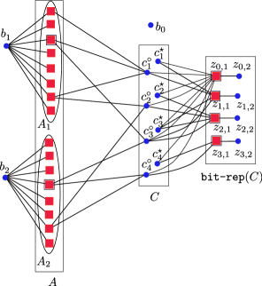
Figure 8: An illustrative example of the graph constructed by the reduction. Red (squared) nodes denote the tests whereas blue (filled circle) nodes the elements. The adjacency across $B$ and $\texttt{bit-rep}(B)$ is same as it was mentioned in Section 3.

This completes the construction. The reduction sets $k=r+|\texttt{bit-rep}(C)|=\mathcal{O}(\log(n))+\mathcal{O}(\log(m))$, and returns $(G,\langle R,B\rangle,k)$ as an instance of Test Cover.

We present a brief overview of the proof of correctness in the reverse direction. Suppose $R^{\prime}$ is a set of tests of the graph $G$ of order at most $k$. Since $b_{0}$ is an isolated blue vertex of $G$, it implies that the set $R^{\prime}$ dominates and locates every pair of vertices in $B\setminus\{b_{0}\}$. The blue vertices in $\texttt{bit-rep}(C)$ are pendant vertices that are adjacent with red vertices in $\texttt{bit-rep}(C)$. Hence, all the red vertices in $\texttt{bit-rep}(C)$ are in $R^{\prime}$. The remaining $r$ many vertices need to locate vertices in pairs ($c^{\circ}_{j}$, $c^{\star}_{j}$), for every $j\in[m]$, which have the same neighbourhood in $\texttt{bit-rep}(C)$. To do so, note that the only vertices adjacent to $c^{\circ}_{j}$ and not to $c^{\star}_{j}$ are in $A_{i}$ and corresponds to an assignment satisfying clause $C_{j}$. Hence, for every $j\in[m]$, the set $R^{\prime}$ should contain at least one vertex $\{a_{i,\ell}$ in order to locate $c^{\circ}_{j}$, $c^{\star}_{j}$, where $(a_{i,\ell},c^{\circ}_{j})$ is an edge for some $i\in[r]$ and $\ell\in[2^{s}]$. Moreover, in order to dominate the vertices of $B$, for each $i\in[r]$, the set $R^{\prime}$ must have a vertex from each $A_{i}$. Hence, the set $R^{\prime}$ is forced to contain exactly one vertex from each $A_{i}$. Concatenating the assignments corresponding to each $a_{i,\ell}$ in $R^{\prime}$, we thus obtain a satisfying assignment of $\psi$. The formal arguments for the correctness follows very closely to the one mentioned in Subsection 4.2.

Proof 7.1 (Proof of Theorem 1.3).

Assume there is an algorithm $\mathcal{A}$ that, given an instance $(G,\langle R,B\rangle,k)$ of Test Cover, runs in time $2^{2^{o(k)}}\cdot(|U|+|\mathcal{F}|)^{\mathcal{O}(1)}$ and correctly determines whether it is Yes-instance. Consider the following algorithm that takes as input an instance $\psi$ of $3$-SAT and determines whether it is a Yes-instance. It first constructs an equivalent instance $(G,\langle R,B\rangle,k)$ of Test Cover  as mentioned in this subsection. Note that such an instance can be constructed in time

Then, it calls algorithm $\mathcal{A}$ as a subroutine and returns the same answer. The correctness of this algorithm follows from the correctness of algorithm $\mathcal{A}$ and the correctness of the reduction. Moreover, from the reduction, we have $k=\mathcal{O}(\log(n)+\log(m))$. As the other steps, including the construction of the instance of Test Cover, can be performed in time $2^{\mathcal{O}(n/\log(n))}\cdot n^{\mathcal{O}(1)}=2^{o(n)}$, the running time of the algorithm for $3$-SAT is $2^{2^{o(\log(n)+\log(m))}}\cdot(|R|+|B|)^{\mathcal{O}(1)}=2^{o(n+m)}\cdot n^{\mathcal{O}(1)}$. This, however, contradicts ETH (using the sparcification lemma). Hence, our assumption is wrong, and Test Cover does not admit an algorithm running in time $2^{2^{o(k)}}\cdot(|U|+|\mathcal{F}|)^{\mathcal{O}(1)}$, unless the ETH fails.

7.3 Parameterization by Treewidth

7.3.1 Upper Bound

In this section, we provide a short sketch of the dynamic programming for Test Cover when parameterized by the treewidth of the bipartite graph of the tests and the items. Consider a bipartite graph $G$ of $n$ vertices with vertex bipartition $\langle R,B\rangle$ of $V(G)$. The objective is to determine whether there is a set of at most $k$ vertices from $R$ such that for each pair $x,y\in B$, there is $r\in R$ such that $rx\in E(G)$ but $ry\notin E(G)$. We assume without loss of generality that we have a nice tree decomposition $\mathcal{T}=(T,\{X_{t}\}_{t\in V(T)})$ of $G$ of width at most $2{\textsf{tw}}(G)+1$. We define $G_{t}$ as before. For every node $t\in V(T)$, we define a subproblem $[t,(Y,W),(\mathcal{A},\mathcal{D}),\mathcal{B}]$ such that ${\texttt{opt}}[t,(Y,W),(\mathcal{A},\mathcal{D}),\mathcal{B}]$ is the size of an optimal solution $S\subseteq R\cap V(G_{t})$ satisfying the following properties.

• $Y=S\cap X_{t}\cap R$ and $W=N_{G_{t}}(S\setminus X_{t})\cap(B\cap X_{t})$,

• $\mathcal{A}\subseteq 2^{Y}$ such that $A\in\mathcal{A}$ if and only if there exists a (unique) $u\in(V(G_{t})\cap B)\setminus(S\cup X_{t})$ such that $N_{G_{t}}(u)\cap S=A$,

• $\mathcal{D}\subseteq 2^{Y}$ such that $A\in\mathcal{D}$ if and only if there exists $u\in(X_{t}\cap B)\setminus S$ such that $N_{G_{t}}(u)\cap S=A$,

• ${\mathcal{B}}\subseteq{{(B\cap X_{t})\setminus Y}\choose{2}}\cup(((B\cap X_{t})\setminus Y)\times\{+\})$ such that (i) a pair of vertices $\{x,y\}\in\mathcal{B}$ if and only if $N_{G_{t}}(x)\cap S=N_{G_{t}}(y)\cap S$, or (ii) $\{x,+\}\in\mathcal{B}$ if and only if there exists $y\in(B\cap V(G_{t}))\setminus(S\cup X_{t})$ such that $N_{G_{t}}(x)\cap S=N_{G_{t}}(y)\cap S$, and

• There do not exist two vertices $y,z\in(B\cap V(G_{t}))\setminus(S\cup X_{t})$ such that $N_{G_{t}}(y)\cap S=N_{G_{t}}(z)\cap S$.

Observe that the DP-states are almost similar to that of Section 5.1. The only difference is that the objective is to pick a smallest size subset of $R$ such that the vertices of $B$ have to be located. We illustrate how the DP works in leaf nodes, introduce nodes, forget nodes, and join nodes. Let $r$ be the root node. Same as before, if we compute the values of

Leaf Node:

Let $t$ be a leaf node and $X_{t}=\emptyset$. Then, the following four types of DP-states are possible. These DP-states are $[t,(\emptyset,\emptyset),(\emptyset,\emptyset),\emptyset]$, $[t,(\emptyset,\emptyset),(\emptyset,\{\emptyset\}),\emptyset]$, $[t,(\emptyset,\emptyset),(\{\emptyset\},\emptyset),\emptyset]$ and $[t,(\emptyset,\emptyset),(\{\emptyset\},\{\emptyset\}),\emptyset]$. Observe that each of the values $\texttt{opt}[t,(\emptyset,\emptyset),(\emptyset,\emptyset),\emptyset]$, $\texttt{opt}[t,(\emptyset,\emptyset),(\emptyset,\{\emptyset\}),\emptyset]$, $\texttt{opt}[t,(\emptyset,\emptyset),(\{\emptyset\},\emptyset),\emptyset]$ and $\texttt{opt}[t,(\emptyset,\emptyset),(\{\emptyset\},\{\emptyset\}),\emptyset]$ are zero since $\emptyset$ is the only set that is a candidate solution for each of these DP-states.

Let $t$ be an introduce/forget node and $t^{\prime}$ be its unique child in $T$. Then, the two DP-states $[t,(Y,W),(\mathcal{A},\mathcal{D}),\mathcal{B}]$ and $[t^{\prime},(Y^{\prime},W^{\prime}),(\mathcal{A}^{\prime},\mathcal{D}^{\prime}),\mathcal{B}^{\prime}]$ are compatible to each other if an optimal solution $S$ to the state $[t,(Y,W),(\mathcal{A},\mathcal{D}),\mathcal{B}]$ satisfies that $S^{\prime}$ is an optimal solution to $[t^{\prime},(Y^{\prime},W^{\prime}),(\mathcal{A}^{\prime},\mathcal{D}^{\prime}),\mathcal{B}^{\prime}]$ such that $S^{\prime}=S\cap V(G_{t^{\prime}})$.

Introduce Node:

Let $t$ be an introduce node such that $t^{\prime}$ is the unique child of $t$ and $X_{t}=X_{t^{\prime}}\cup\{u\}$. Similar as in the case of Locating-Dominating Set, if $Y^{\prime}\neq Y$ and $Y^{\prime}\neq Y\setminus\{u\}$, then the DP-states $[t,(Y,W),(\mathcal{A},\mathcal{D}),\mathcal{B}]$ and $[t^{\prime},(Y^{\prime},W^{\prime}),(\mathcal{A}^{\prime},\mathcal{D}^{\prime}),\mathcal{B}^{\prime}]$ are not compatible to each other. Consider the set $\mathcal{C}$ of all the DP-states $[t^{\prime},(Y^{\prime},W^{\prime}),(\mathcal{A}^{\prime},\mathcal{D}^{\prime}),\mathcal{B}^{\prime}]$ for the node $t^{\prime}$ that are compatible to the DP-state $[t,(Y,W),(\mathcal{A},\mathcal{D}),\mathcal{B}]$. Using arguments similar to Section 5.1, we can prove that if $u\in R$, then

$${\texttt{opt}}[t,(Y,W),(\mathcal{A},\mathcal{D}),\mathcal{B}]=1+\min\limits_{\mathcal{C}}[t^{\prime},(Y^{\prime},W^{\prime}),(\mathcal{A}^{\prime},\mathcal{D}^{\prime}),\mathcal{B}^{\prime}]$$

Otherwise, if $u\in B$, then

$${\texttt{opt}}[t,(Y,W),(\mathcal{A},\mathcal{D}),\mathcal{B}]=\min\limits_{\mathcal{C}}[t^{\prime},(Y^{\prime},W^{\prime}),(\mathcal{A}^{\prime},\mathcal{D}^{\prime}),\mathcal{B}^{\prime}]$$

Forget Node:

Let $t$ be a forget node such that $t^{\prime}$ be its unique chid. Same as before, consider the set $\mathcal{C}$ of all the DP-states that are compatible to the DP-state $[t,(Y,W),(\mathcal{A},\mathcal{D}),\mathcal{B}]$. Since an optimal solution to $[t,(Y,W),(\mathcal{A},\mathcal{D}),\mathcal{B}]$ is the same as an optimal solution to $[t^{\prime},(Y^{\prime},W^{\prime}),(\mathcal{A}^{\prime},\mathcal{D}^{\prime}),\mathcal{B}]$, we can prove in a similar way that

$${\texttt{opt}}[t,(Y,W),(\mathcal{A},\mathcal{D}),\mathcal{B}]=\min\limits_{\mathcal{C}}[t^{\prime},(Y^{\prime},W^{\prime}),(\mathcal{A}^{\prime},\mathcal{D}^{\prime}),\mathcal{B}^{\prime}]$$

Join Node:

Let $t$ be a join node with its two children $t_{1}$ and $t_{2}$. To compute the value of ${\texttt{opt}}[t,(Y,W),(\mathcal{A},\mathcal{D}),\mathcal{B}]$, we consider the collection of all DP-states $[t_{1},(Y_{1},W_{1}),(\mathcal{A}_{1},\mathcal{D}_{1}),\mathcal{B}_{1}]$ and $[t_{2},(Y_{2},W_{2}),(\mathcal{A}_{2},\mathcal{D}_{2}),\mathcal{B}_{2}]$ such that the three above mentioned states are compatible to each other. By arguments similar as before, we can justify that

$${\texttt{opt}}[t,(Y,W),(\mathcal{A},\mathcal{D}),\mathcal{B}]$$

$$=\min_{\mathcal{C}}\bigg{\{}{\texttt{opt}}[t_{1},(Y_{1},W_{1}),(\mathcal{A}_{1},\mathcal{D}_{1}),\mathcal{B}_{1}]+{\texttt{opt}}[t_{2},(Y_{2},W_{2}),(\mathcal{A}_{2},\mathcal{D}_{2}),\mathcal{B}_{2}]-|Y|\bigg{\}}$$

Finally, by similar arguments as before, we can prove that Test Cover can be solved in time $2^{2^{\mathcal{O}(\textsf{tw})}}n^{\mathcal{O}(1)}$.

7.3.2 Lower Bound

In this subsection, we prove the lower bound mentioned in Theorem 1.4, i.e., Test Cover does not admit an algorithm running in time $2^{2^{o(tw)}}\cdot|V(G)|^{\mathcal{O}(1)}$, unless the ETH fails. We present a reduction which is a modification of the reduction presented in Subsection 5.2.

Reduction

For notational convenience, instead of specify an instance of Test Cover, we specify the auxiliary graph as mentioned in the definition. The reduction takes as input an instance $\psi$ of $(3,3)$-SAT with $n$ variables and outputs an instance $(G,\langle R,B\rangle,k)$ of Test Cover such that $\textsf{tw}(G)=\mathcal{O}(\log(n))$. Suppose $X=\{x_{1},\dots,x_{n}\}$ is the collection of variables and $C=\{C_{1},\dots,C_{m}\}$ is the collection of clauses in $\psi$. Here, we consider $\langle x_{1},\dots,x_{n}\rangle$ and $\langle C_{1},\dots,C_{m}\rangle$ be arbitrary but fixed orderings of variables and clauses in $\psi$. For a particular clause, the first order specifies the first, second, or third (if it exists) variable in the clause in a natural way. The second ordering specifies the first/second positive/negative appearance of variables in $X$ in a natural way. The reduction constructs a graph $G$ as follows after initialising $R=B=\emptyset$.

• To construct a variable gadget for $x_{i}$, it adds a blue vertex $\beta_{i}$ to $B$, two red vertices $\alpha^{1}_{i},\alpha^{2}_{i}$ to $R$, and four blue vertices $x_{i}^{1},\neg x_{i}^{1},x_{i}^{2},\neg x_{i}^{2}$ to $B$. It then adds the edges as shown in Figure 9. Let $A_{i}$ be the collection of these seven vertices. Define $X_{i}:=\{x_{i}^{1},\neg x_{i}^{1},x_{i}^{2},\neg x_{i}^{2}\}$.

• To construct a clause gadget for $C_{j}$, the reduction adds three blue vertices $\{\gamma_{j}^{1},\gamma_{j}^{2},\gamma_{j}^{3}\}$ to $B$, three red vertices $\{\delta_{j}^{1},\delta_{j}^{2},\delta_{j}^{3}\}$ to $R$, and three vertices $c^{1}_{j},c^{2}_{j},c^{3}_{j}$ to $B$. It adds the edges as shown in Figure 9. Let $B_{j}$ be the collection of these nine vertices.

• Let $p$ be the smallest positive integer such that $4n\leq\binom{2p}{p}$. Define $\mathcal{F}_{p}$ as the collection of subsets of $[2p]$ that contains exactly $p$ integers (such a collection $\mathcal{F}_{p}$ is called a Sperner family). Define $\texttt{set-rep}:\bigcup_{i=1}^{n}X_{i}\mapsto\mathcal{F}_{p}$ as an injective function by arbitrarily assigning a set in $\mathcal{F}_{p}$ to a vertex $x^{\ell}_{i}$ or $\neg x^{\ell}_{i}$, for every $i\in[n]$ and $\ell\in[2]$. In other words, every appearance of a literal is assigned a distinct subset in $\mathcal{F}_{p}$.

• The reduction adds a connection portal $V$, which is an independent set on $2p$ red vertices $v_{1},v_{2},\dots,v_{2p}$, to $R$. For every vertex $v_{q}$ in $V$, the reduction adds a pendant blue vertex $u_{q}$ adjacent to the red vertex $v_{q}$.

• For all vertex $x_{i}^{\ell}\in X$ where $i\in[n]$ and $\ell\in[2]$, the reduction adds edges $(x^{\ell}_{i},v_{q})$ for every $q\in\texttt{set-rep}(x^{\ell}_{i})$. Similarly, it adds edges $(\neg x^{\ell}_{i},v_{q})$ for every $q\in\texttt{set-rep}(\neg x^{\ell}_{i})$.

• For a clause $C_{j}$, suppose variable $x_{i}$ appears positively for the $\ell^{th}$ time as the $r^{th}$ variable in $C_{j}$. For example, $x_{i}$ appears positively for the second time as the third variable in $C_{j}$. Then, the reduction adds edges across $B$ and $V$ such that the vertices $c_{j}^{r}$ and $x^{\ell}_{i}$ have the same neighbourhood in $V$, namely, the set $\{v_{q}:q\in\texttt{set-rep}(x^{\ell}_{i})\}$. Similarly, it adds edges for the negative appearance of the variables.

• The reduction adds an isolated blue vertex $x_{0}$.

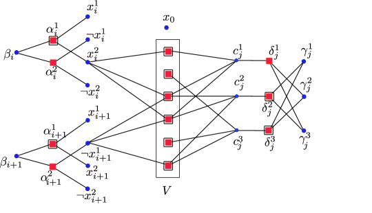
Figure 9: An illustrative example of the graph constructed by the reduction. Red (squared) nodes denote the tests whereas blue (filled circle) nodes the elements. For the sake of clarity, we do not explicitly show the pendant blue vertices adjacent to vertices in $V$. The variable and clause gadgets are on the left-side and right-side of $V$, respectively. This is an adaptation of the same example mentioned in Subsection 5.2. The rectangle boundary around the red vertices denotes a solution.

This concludes the construction of $G$. The reduction sets $k=n+2m+2p$ and returns $(G,\langle R,B\rangle,k)$ as the reduced instance of Test Cover.

We now provide an overview of the proof of correctness in the reverse direction. The crux of the correctness is: Without loss of generality, all the red vertices in the connection portal $V$ are present in any test cover $T$ of $G$. Consider a blue vertex, say $x^{1}_{i}$, on ‘variable-side’ of $T$ and a blue vertex, say $c^{1}_{j}$, on ‘clause-side’ of $T$, and suppose they have same neighbors in the connection portal. Then, at least $x^{1}_{i}$ is adjacent with red vertices in $T\setminus V$ or $c^{1}_{j}$ is adjacent with red vertices in $S\setminus V$.

More formally, suppose $T$ is a test cover of $G$ of size $k=n+2m+2p$. As every vertex in $V$ is present in $T$, we know that $T$ contains exactly one and exactly 2 vertices from each variable gadget and clause gadget, respectively. This is ensured by the fact that there is an isolated blue vertex $x_{0}$, and the blue vertex $\beta_{i}$ is adjacent with only two red vertices viz $\alpha^{1}_{i}$ and $\alpha^{2}_{i}$. Hence, at least one of them is in $T$. Similarly, three blue vertices $\{\gamma_{j}^{1},\gamma_{j}^{2},\gamma_{j}^{3}\}$ and their adjacency with three red vertices in $\{\delta_{j}^{1},\delta_{j}^{2},\delta_{j}^{3}\}$, ensures at least two vertices from the later set should be in $T$. Selecting $\alpha^{1}_{i}$ corresponds to setting the variable to True and seleting $\alpha^{2}_{i}$ corresponding to setting the variable to False. Also, including $\{\delta_{j}^{2},\delta_{j}^{3}\}$, $\{\delta_{j}^{1},\delta_{j}^{3}\}$, and $\{\delta_{j}^{1},\delta_{j}^{2}\}$ in $T$, corresponding to selecting the first, second and the third variable, respectively, to satisfy clause $C_{j}$. As in Subsection 5.2, the connection portal and its adjacencies to variable gadgets and clause gadgets ensures that these choices are consistent.

This establishes the correctness of the reduction. The argument regarding the conditional lower bound is identical as in Subsection 5.2.

7.4 Parameterization by the Number of Elements

Red-Blue Locating Set admits a simple $|R|^{\mathcal{O}(k)}\cdot(|R|+|B|)^{\mathcal{O}(1)}$ algorithm that enumerates all the possible subsets of $R$ and checks it for feasibility. Our goal is find an  algorithm parameterized by $|B|$. Note that it is safe to assume $|R|\leq 2^{|B|}$ (since we can remove twin vertices from $R$ and get an equivalent instance) and $k\leq|B|$ by Bondy’s theorem [8] (which asserts that Test Cover always has a solution of size at most $|B|-1$). Hence, the brute-force algorithm mentioned above runs in time $2^{\mathcal{O}(|B|^{2})}\cdot(|R|+|B|)^{\mathcal{O}(1)}$.

In what follows, our objective is present an improved  algorithm, in the spirit of the known $\mathcal{O}(mn2^{n})$ dynamic programming scheme for Set Cover on a universe of size $n$ and $m$ sets (see [26, Theorem 3.10]). We next restate the theorem.

See 1.6

To prove it, it suffices to apply Lemma 6.5. Indeed, we reduce Red-Blue Locating Set to Annotated Red-Blue Partition Refinement. For this, note that in a solution of Red-Blue Locating Set, either every vertex of $B$ is dominated by the solution, or exactly one vertex of $B$ is not dominated by the solution. Thus, we go through every possible choice of subset $T_{L}\subseteq B$ with $|T_{L}|\in\{|B-|-1,|B|\}$. We let $C_{0}=\emptyset$, and define the partition $\mathcal{Q}$ defined by taking all vertices of $R$ as parts of size 1, and the set $B$ as the last part. Now, it suffices to run the dynamic programming for solving Annotated Red-Blue Partition Refinement with each fof the $|B|+1$ choices of set $T_{L}$, giving a running time of $2^{\mathcal{O}(|B|\log|B|)}\cdot(|R|+|B|)^{\mathcal{O}(1)}$.

8 Conclusion

In this article, we presented several results that advances our understanding of the algorithmic complexity of Locating-Dominating Set and Test Cover. Moreover, we believe the techniques used in this article can be applied to other identification problems to obtain relatively rare conditional lower bounds. The process of establishing such lower bounds boils down to designing bit-representation gadget and set-representation gadget for the problem in question.

Apart from the broad question of designing such lower bounds for other identification problems, we list a few interesting problems left open by our work. We have the $2^{2^{\mathcal{O}(k)}}$ kernel for Test Cover but the $2^{o(k)}$ lower bound. It would be interesting to reduce this gap. Another interesting question is whether our tight double-exponential lower bound for Locating-Dominating Set parameterized by treewidth/treedepth can be applied to the feedback vertex set number. We do not know whether our slightly superexponential  algorithm for Locating-Dominating Set parameterized by vertex cover (and similarly, the algorithm for Test Cover parameterized by $|B|$) is optimal, or whether there exists a single-exponential algorithm with respect to vertex cover. Another open question in this direction, is whether this algorithm, which can be extended to twin-cover, can be generalized even further to the distance to cluster. The approach from [10, 11] gives only a double-exponential kernel, and thus, a triple-exponential  algorithm. As our linear kernel for parameter feedback edge set is not explicit, it would be nice to obtain a concrete kernel. For that, one should find a way to define the gadgets explicitly. This is easy to do for the five gadgets from Definition 6.18. However, as the number of possible gadgets from Definition 6.27 is huge, one should probably design a different kernelization algorithm.

References

- [1] A. Agrawal, D. Lokshtanov, S. Saurabh, and M. Zehavi. Split contraction: The untold story. ACM Trans. Comput. Theory, 11(3):18:1–18:22, 2019.
- [2] Akanksha Agrawal, Lawqueen Kanesh, Saket Saurabh, and Prafullkumar Tale. Paths to trees and cacti. Theor. Comput. Sci., 860:98–116, 2021. URL: https://doi.org/10.1016/j.tcs.2021.01.033, doi:10.1016/J.TCS.2021.01.033.
- [3] Gabriela R. Argiroffo, Silvia M. Bianchi, Yanina Lucarini, and Annegret Katrin Wagler. Linear-time algorithms for three domination-based separation problems in block graphs. Discret. Appl. Math., 281:6–41, 2020.
- [4] L. Babai. On the complexity of canonical labelling of strongly regular graphs. SIAM J. Comput., 9(1):212–216, 1980.
- [5] Florian Barbero, Lucas Isenmann, and Jocelyn Thiebaut. On the distance identifying set meta-problem and applications to the complexity of identifying problems on graphs. Algorithmica, 82(8):2243–2266, 2020.
- [6] Manu Basavaraju, Mathew C. Francis, M. S. Ramanujan, and Saket Saurabh. Partially polynomial kernels for set cover and test cover. SIAM J. Discret. Math., 30(3):1401–1423, 2016.
- [7] Piotr Berman, Bhaskar DasGupta, and Ming-Yang Kao. Tight approximability results for test set problems in bioinformatics. J. Comput. Syst. Sci., 71(2):145–162, 2005.
- [8] John A Bondy. Induced subsets. Journal of Combinatorial Theory, Series B, 12(2):201–202, 1972.
- [9] Koen M. J. De Bontridder, Bjarni V. Halldórsson, Magnús M. Halldórsson, Cor A. J. Hurkens, Jan Karel Lenstra, R. Ravi, and Leen Stougie. Approximation algorithms for the test cover problem. Math. Program., 98(1-3):477–491, 2003.
- [10] Márcia R. Cappelle, Guilherme de C. M. Gomes, and Vinícius Fernandes dos Santos. Parameterized algorithms for locating-dominating sets. CoRR, abs/2011.14849, 2020. URL: https://arxiv.org/abs/2011.14849, arXiv:2011.14849.
- [11] Márcia R. Cappelle, Guilherme C. M. Gomes, and Vinícius Fernandes dos Santos. Parameterized algorithms for locating-dominating sets. In Carlos E. Ferreira, Orlando Lee, and Flávio Keidi Miyazawa, editors, Proceedings of the XI Latin and American Algorithms, Graphs and Optimization Symposium, LAGOS 2021, Online Event / São Paulo, Brazil, May 2021, volume 195 of Procedia Computer Science, pages 68–76. Elsevier, 2021.
- [12] Jérémie Chalopin, Victor Chepoi, Fionn Mc Inerney, and Sébastien Ratel. Non-clashing teaching maps for balls in graphs. CoRR, abs/2309.02876, 2023. URL: https://doi.org/10.48550/arXiv.2309.02876, arXiv:2309.02876, doi:10.48550/ARXIV.2309.02876.
- [13] L. S. Chandran, D. Issac, and A. Karrenbauer. On the parameterized complexity of biclique cover and partition. In J. Guo and D. Hermelin, editors, 11th International Symposium on Parameterized and Exact Computation, IPEC 2016, volume 63 of LIPIcs, pages 11:1–11:13. Schloss Dagstuhl - Leibniz-Zentrum für Informatik, 2016.
- [14] Emmanuel Charbit, Irène Charon, Gérard D. Cohen, Olivier Hudry, and Antoine Lobstein. Discriminating codes in bipartite graphs: bounds, extremal cardinalities, complexity. Advances in Mathematics of Communication, 2(4):403–420, 2008.
- [15] Irène Charon, Gérard D. Cohen, Olivier Hudry, and Antoine Lobstein. Discriminating codes in (bipartite) planar graphs. Eur. J. Comb., 29(5):1353–1364, 2008.
- [16] Bogdan S. Chlebus and Sinh Hoa Nguyen. On finding optimal discretizations for two attributes. In Proceedings of the First International Conference on Rough Sets and Current Trends in Computing, volume 1424, pages 537–544, Berlin, Heidelberg, 1998. Springer Berlin Heidelberg.
- [17] C. Colbourn, P. J. Slater, and L. K. Stewart. Locating-dominating sets in series-parallel networks. Congressus Numerantium, 56:135–162, 1987.
- [18] David Coudert, Guillaume Ducoffe, and Alexandru Popa. Fully polynomial FPT algorithms for some classes of bounded clique-width graphs. ACM Trans. Algorithms, 15(3):33:1–33:57, 2019. doi:10.1145/3310228.
- [19] Bruno Courcelle. The monadic second-order logic of graphs. I. Recognizable sets of finite graphs. Information and Computation, 85(1):12–75, 1990.
- [20] Bruno Courcelle, Johann A. Makowsky, and Udi Rotics. Linear time solvable optimization problems on graphs of bounded clique-width. Theory Comput. Syst., 33(2):125–150, 2000.
- [21] Robert Crowston, Gregory Z. Gutin, Mark Jones, Gabriele Muciaccia, and Anders Yeo. Parameterizations of test cover with bounded test sizes. Algorithmica, 74(1):367–384, 2016.
- [22] Robert Crowston, Gregory Z. Gutin, Mark Jones, Saket Saurabh, and Anders Yeo. Parameterized study of the test cover problem. In Branislav Rovan, Vladimiro Sassone, and Peter Widmayer, editors, Mathematical Foundations of Computer Science 2012 - 37th International Symposium, MFCS 2012, Bratislava, Slovakia, August 27-31, 2012. Proceedings, volume 7464 of Lecture Notes in Computer Science, pages 283–295. Springer, 2012.
- [23] M. Cygan, M. Pilipczuk, and M. Pilipczuk. Known algorithms for edge clique cover are probably optimal. SIAM J. Comput., 45(1):67–83, 2016.
- [24] Marek Cygan, Fedor V. Fomin, Lukasz Kowalik, Daniel Lokshtanov, Dániel Marx, Marcin Pilipczuk, Michal Pilipczuk, and Saket Saurabh. Parameterized Algorithms. Springer, 2015. doi:10.1007/978-3-319-21275-3.
- [25] Reinhard Diestel. Graph Theory, 4th Edition, volume 173 of Graduate texts in mathematics. Springer, 2012. URL: https://dblp.org/rec/books/daglib/0030488.bib.
- [26] Fedor V. Fomin and Dieter Kratsch. Exact Exponential Algorithms. Texts in Theoretical Computer Science. An EATCS Series. Springer, 2010. doi:10.1007/978-3-642-16533-7.
- [27] Fedor V Fomin, Daniel Lokshtanov, Saket Saurabh, and Meirav Zehavi. Kernelization: theory of parameterized preprocessing. Cambridge University Press, 2019.
- [28] Florent Foucaud. Decision and approximation complexity for identifying codes and locating-dominating sets in restricted graph classes. J. Discrete Algorithms, 31:48–68, 2015.
- [29] Florent Foucaud, Esther Galby, Liana Khazaliya, Shaohua Li, Fionn Mc Inerney, Roohani Sharma, and Prafullkumar Tale. Problems in NP can admit double-exponential lower bounds when parameterized by treewidth and vertex cover. CoRR, abs/2307.08149, 2023. URL: https://doi.org/10.48550/arXiv.2307.08149, arXiv:2307.08149, doi:10.48550/ARXIV.2307.08149.
- [30] Florent Foucaud, George B. Mertzios, Reza Naserasr, Aline Parreau, and Petru Valicov. Identification, location-domination and metric dimension on interval and permutation graphs. I. bounds. Theoretical Computer Science, 668:43–58, 2017.
- [31] Florent Foucaud, George B Mertzios, Reza Naserasr, Aline Parreau, and Petru Valicov. Identification, location-domination and metric dimension on interval and permutation graphs. II. algorithms and complexity. Algorithmica, 78(3):914–944, 2017.
- [32] Robert Ganian. Twin-cover: Beyond vertex cover in parameterized algorithmics. In Dániel Marx and Peter Rossmanith, editors, Parameterized and Exact Computation - 6th International Symposium, IPEC 2011, Saarbrücken, Germany, September 6-8, 2011. Revised Selected Papers, volume 7112 of Lecture Notes in Computer Science, pages 259–271. Springer, 2011. doi:10.1007/978-3-642-28050-4\_21.
- [33] M. R. Garey and D. S. Johnson. Computers and Intractability - A guide to NP-completeness. W.H. Freeman and Company, 1979.
- [34] Sylvain Gravier, Ralf Klasing, and Julien Moncel. Hardness results and approximation algorithms for identifying codes and locating-dominating codes in graphs. Algorithmic Oper. Res., 3(1), 2008. URL: http://journals.hil.unb.ca/index.php/AOR/article/view/2808.
- [35] Gregory Z. Gutin, Gabriele Muciaccia, and Anders Yeo. (non-)existence of polynomial kernels for the test cover problem. Inf. Process. Lett., 113(4):123–126, 2013.
- [36] Michel Habib, Christophe Paul, and Laurent Viennot. A synthesis on partition refinement: A useful routine for strings, graphs, boolean matrices and automata. In Proceedings of the 15th Annual Symposium on Theoretical Aspects of Computer Science (STACS 1998), pages 25–38, Berlin, Heidelberg, 1998. Springer-Verlag.
- [37] A. Ian. Combinatorics of Finite Sets. Oxford University Press, 1987.
- [38] Russell Impagliazzo and Ramamohan Paturi. On the complexity of k-sat. J. Comput. Syst. Sci., 62(2):367–375, 2001. URL: https://doi.org/10.1006/jcss.2000.1727, doi:10.1006/JCSS.2000.1727.
- [39] Russell Impagliazzo, Ramamohan Paturi, and Francis Zane. Which problems have strongly exponential complexity? J. Comput. Syst. Sci., 63(4):512–530, 2001. URL: https://doi.org/10.1006/jcss.2001.1774, doi:10.1006/JCSS.2001.1774.
- [40] Bart M. P. Jansen and Astrid Pieterse. Sparsification upper and lower bounds for graph problems and not-all-equal SAT. Algorithmica, 79(1):3–28, 2017. URL: https://doi.org/10.1007/s00453-016-0189-9, doi:10.1007/S00453-016-0189-9.
- [41] Leon Kellerhals and Tomohiro Koana. Parameterized complexity of geodetic set. J. Graph Algorithms Appl., 26(4):401–419, 2022.
- [42] T. Kloks. Treewidth, Computations and Approximations. Springer, 1994.
- [43] T. Korhonen. A single-exponential time 2-approximation algorithm for treewidth. In 2021 IEEE 62nd Annual Symposium on Foundations of Computer Science (FOCS 2021), pages 184–192, 2022.
- [44] S. Kratsch, G. Philip, and S. Ray. Point line cover: The easy kernel is essentially tight. ACM Trans. Algorithms, 12(3):40:1–40:16, 2016.
- [45] Michael Lampis. Algorithmic meta-theorems for restrictions of treewidth. Algorithmica, 64(1):19–37, 2012. URL: https://doi.org/10.1007/s00453-011-9554-x, doi:10.1007/S00453-011-9554-X.
- [46] Daniel Lokshtanov, Dániel Marx, and Saket Saurabh. Known algorithms on graphs of bounded treewidth are probably optimal. ACM Trans. Algorithms, 14(2):13:1–13:30, 2018.
- [47] Bernard M. E. Moret and Henry D. Shapiro. On minimizing a set of tests. SIAM Journal on Scientific and Statistical Computing, 6(4):983–1003, 1985.
- [48] Tobias Müller and Jean-Sébastien Sereni. Identifying and locating-dominating codes in (random) geometric networks. Comb. Probab. Comput., 18(6):925–952, 2009.
- [49] M. Pilipczuk. Problems parameterized by treewidth tractable in single exponential time: A logical approach. In Mathematical Foundations of Computer Science 2011 - 36th International Symposium, MFCS 2011, Proceedings, volume 6907 of Lecture Notes in Computer Science, pages 520–531. Springer, 2011.
- [50] N.S.V. Rao. Computational complexity issues in operative diagnosis of graph-based systems. IEEE Transactions on Computers, 42(4):447–457, 1993.
- [51] Alfred Rényi. On random generating elements of a finite boolean algebra. Acta Scientiarum Mathematicarum Szeged, 22:75–81, 1961.
- [52] I. Sau and U. dos Santos Souza. Hitting forbidden induced subgraphs on bounded treewidth graphs. Inf. Comput., 281:104812, 2021.
- [53] Peter J. Slater. Domination and location in acyclic graphs. Networks, 17(1):55–64, 1987. doi:10.1002/net.3230170105.
- [54] Peter J. Slater. Domination and location in acyclic graphs. Networks, 17(1):55–64, 1987.
- [55] Peter J. Slater. Dominating and reference sets in a graph. Journal of Mathematical and Physical Sciences, 22(4):445–455, 1988.
- [56] Jukka Suomela. Approximability of identifying codes and locating-dominating codes. Inf. Process. Lett., 103(1):28–33, 2007. URL: https://doi.org/10.1016/j.ipl.2007.02.001, doi:10.1016/J.IPL.2007.02.001.
- [57] Craig A. Tovey. A simplified np-complete satisfiability problem. Discret. Appl. Math., 8(1):85–89, 1984. doi:10.1016/0166-218X(84)90081-7.
- [58] Johan M. M. van Rooij, Hans L. Bodlaender, and Peter Rossmanith. Dynamic programming on tree decompositions using generalised fast subset convolution. In Amos Fiat and Peter Sanders, editors, Algorithms - ESA 2009, 17th Annual European Symposium, Copenhagen, Denmark, September 7-9, 2009. Proceedings, volume 5757 of Lecture Notes in Computer Science, pages 566–577. Springer, 2009.