Abstract

Training Deep Neural Networks (DNNs) with small batches using Stochastic Gradient Descent (SGD) yields superior test performance compared to larger batches. The specific noise structure inherent to SGD is known to be responsible for this implicit bias. DP-SGD, used to ensure differential privacy (DP) in DNNs’ training, adds Gaussian noise to the clipped gradients. Surprisingly, large-batch training still results in a significant decrease in performance, which poses an important challenge because strong DP guarantees necessitate the use of massive batches. We first show that the phenomenon extends to Noisy-SGD (DP-SGD without clipping), suggesting that the stochasticity (and not the clipping) is the cause of this implicit bias, even with additional isotropic Gaussian noise. We theoretically analyse the solutions obtained with continuous versions of Noisy-SGD for the Linear Least Square and Diagonal Linear Network settings, and reveal that the implicit bias is indeed amplified by the additional noise. Thus, the performance issues of large-batch DP-SGD training are rooted in the same underlying principles as SGD, offering hope for potential improvements in large batch training strategies.

1 Introduction

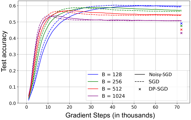
Figure 1: Training from scratch on ImageNet for $S=72k$ steps, using a constant learning rate, with different batch sizes $B$. The effective noise $\sigma/B$ is constant within DP-SGD and Noisy-SGD experiments. The crosses for DP-SGD are obtained from Sander et al. (2023). We observe a similar phenomenon for the non-clipped version (Noisy-SGD), i.e., small batches perform better that larger ones, suggesting that clipping is not solely responsible. Even with isotropic noise added with greater magnitude than the gradients, SGD’s implicit bias persists: the natural noise structure in SGD is robust to Gaussian perturbations.

In Machine Learning, the Gradient Descent (GD) algorithm is used to minimize an empirical loss function by iteratively updating the model parameters in the direction opposite to the gradient. Its stochastic variant, Stochastic Gradient Descent (SGD) (Robbins and Monro, 1951; Duflo, 1996) uses a random subset of the training data at each step, known as a mini-batch, to estimate the true gradient. It enables the training of machine learning models on vast datasets or with extremely large models, where the computation of the full gradient becomes too computationally intensive. Especially in Deep Learning, SGD or its variant has proven to be a crucial tool for training DNNs, delivering exceptional performance across various domains including computer vision (He et al., 2016), natural language processing (Devlin et al., 2018; Touvron et al., 2023), and speech recognition (Amodei et al., 2016).

SGD can achieve better performance than GD under a fixed compute budget (i.e., number of epochs), as well as at a fixed number of steps budget (i.e., number of updates) (Keskar et al., 2016; Smith et al., 2020; Masters and Luschi, 2018). Consequently, not only does SGD offer significant computational resource savings, but its inherent stochastic nature introduces randomness into the algorithm which facilitates faster convergence and enhance generalization performance, by allowing the iterates to escape from unfavorable local minima. On simpler, overparameterized model architectures, the distinctive noise structure of SGD is recognized as a factor responsible for yielding superior solutions compared to Gradient Descent, which is referred to as its “implicit bias” (HaoChen et al., 2020).

DNNs possess the ability to grasp the general statistical patterns and trends within their training data distribution —such as grammar rules for language models— but also to memorize specific and precise details about individual data points, including sensitive information like credit card numbers (Carlini et al., 2019, 2021). This capability raises concerns regarding privacy, as accessing a trained model may lead to the exposure of training data, potentially jeopardizing privacy. One possible solution to address this issue is Differential Privacy (DP) (Dwork et al., 2006), which theoretically controls the amount of information learned from each individual training sample.

Differentially Private Stochastic Gradient Descent (DP-SGD) (Abadi et al., 2016) offers a robust framework by providing strict DP guarantees for DNNs. The gradient of each training sample is clipped and Gaussian noise is subsequently introduced to the sum before the update. Efforts to enhance the trade-off between privacy and utility in DP-SGD training have been associated with the use of exceedingly large batches (Yu et al., 2021; De et al., 2022; Yu et al., 2023). A recent observation by Sander et al. (2023) has introduced an intriguing challenge: under the same Gaussian noise, small batches perform considerably better than large batches, akin to the behavior of regular SGD. It represents a bottleneck because large-batch training is essential for achieving robust privacy guarantees.

DP-SGD distinguishes itself from SGD by two factors: (1) the application of per-sample gradient clipping and (2) the addition of isotropic Gaussian noise to the sum per batch. We first observe a persistent manifestation of the implicit bias associated with DP-SGD observed by Sander et al. (2023) when we remove the gradient clipping component, as depicted in Figure 1. Therefore, the implicit bias of SGD does persist even with Gaussian noise with greater magnitude than the gradients (see Figure 2). However, the implicit bias in SGD is conventionally understood to stem from its inherent noise geometry (HaoChen et al., 2020). In this context, we theoretically investigate the impact of changing the noise structure of SGD on its implicit bias, in the Linear Least Square and Diagonal Linear network (DLN) settings. Our precise contributions are the following:

1. We show that the performance drop observed for large batch training in DP-SGD persists without clipping when training a DNN on ImageNet

2. For Linear Least Squares, we show how Noisy-SGD alters the limiting distributions: the different implicit bias compared to SGD can be controlled by the amount of additional noise

3. For DLNs, we observe that Noisy-SGD can even exhibit an enhanced implicit bias in comparison to SGD. Using continuous modelings, we theoretically demonstrate that a favorable implicit bias indeed exists: It leads to the same solution as SGD, albeit with a distinct effective initialization.

It proves that the gradient’s noise geometry is robust to Gaussian perturbations. Our work also suggests that enhancing the performance of large batch training with DP-SGD, which is crucial for achieving robust privacy-utility trade-off, can be accomplished by adopting strategies and techniques developed for managing large batches in non-private settings.

2 Background and Related Work

2.1 Differential Privacy

General Introduction

$\mathcal{M}$ is a mechanism that takes as input a dataset $D$ and outputs a machine learning model $\theta\sim\mathcal{M}(D)$.

Definition 1 (Approximate Differential Privacy).

A randomized mechanism $\mathcal{M}$ satisfies $(\varepsilon,\delta)$-DP (Dwork et al., 2006) if, for any pair of datasets $D$ and $D^{\prime}$ that differ by one sample and for all subset $R\subset\mathbf{Im}(\mathcal{M})$,

$$\mathbb{P}(\mathcal{M}(D)\in R)\leq\mathbb{P}(\mathcal{M}(D^{\prime})\in R)\exp(\varepsilon)+\delta.$$ (1)

Differential Privacy (DP) safeguards against the ability of any potential adversary to infer information about the dataset $\mathcal{D}$ once they’ve observed the output of the algorithm. In machine learning, this concept implies that if someone acquires the model’s parameter $\bm{\theta}$ trained with a DP algorithm $\mathcal{M}$, then the training data is, by provable guarantees, difficult to reconstruct or infer (Balle et al., 2022; Guo et al., 2022, 2023).

DP-SGD

(Chaudhuri et al., 2011; Abadi et al., 2016) is the most popular DP algorithm to train DNNs. It first selects samples uniformly at random with probability $q=B/N$. For $C>0$, define the clipping function for any $X\in\mathbb{R}^{d}$ by $\mathrm{clip}_{C}(X)=C\cdot X/\|X\|$ if $\|X\|\geq C$ and $\mathrm{clip}_{C}(X)=X$ otherwise. DP-SGD clips the per sample gradients, aggregates them and adds Gaussian noise. Given model parameters $\bm{\theta}_{k}$, DP-SGD defines the update $\bm{\theta}_{k+1}=\bm{\theta}_{k}-\eta_{k}\widetilde{\mathbf{g}}_{k}$ where $\eta_{k}$ is the step size and $\widetilde{\mathbf{g}}_{k}$ is given by:

$$\widetilde{\mathbf{g}}_{k}:=\frac{1}{B}\sum_{i\in\mathcal{B}_{k}}\text{clip}_{C}\left(\nabla_{\bm{\theta}}\ell_{i}(\bm{\theta}_{k})\right)+\mathcal{N}\left(0,C^{2}\frac{\sigma^{2}}{B^{2}}\mathbf{I}\right).$$ (2)

$\ell_{i}(\bm{\theta})$ represents the individual loss function computed for the sample $\mathbf{x}_{i}$. The privacy analysis of DP-SGD hinges on the combination of multiple steps. A notably robust analytical framework to account for $(\varepsilon,\delta)$ is founded on Rényi differential privacy (Mironov, 2017). The theoretical analysis of the convergence properties of DP-SGD has been studied for the convex, strongly convex, and nonconvex settings (Bassily et al., 2014; Wang et al., 2017; Feldman et al., 2018).

Necessity of Large batches for DP-SGD

When it comes to training machine learning models with DP-SGD, there is necessarily a privacy-performance trade-off. However, it can be improved by employing very large batch sizes (Anil et al., 2021; Li et al., 2021; De et al., 2022; Yu et al., 2023).

One practical underlying reason is that the magnitude of the effective noise introduced into the average clipped gradient is determined by $\sigma/B$ (cf. Equation (2)). To mitigate this noise, there are two potential approaches: reducing $\sigma$ or increasing $B$. While decreasing $\sigma$ might initially appear appealing, Rényi differential privacy accounting techniques suggest that as $\sigma$ decreases too much, the privacy parameter $\varepsilon$ experiences an exponential increase (Dwork and Rothblum, 2016; Bun and Steinke, 2016; Mironov et al., 2019; Sander et al., 2023). Therefore, increasing the batch size emerges as a critical strategy in DP-SGD training, as it is the most effective means of reducing the effective noise and accelerating the convergence process.

While it is true that employing a larger batch size in DP-SGD results in reduced effective noise, it is important to note that DP training can experience a substantial drop in performance when using larger batch sizes. As demonstrated by Sander et al. (2023), when training an image classifier with DP-SGD on the ImageNet dataset, keeping the number of steps $S$ fixed and maintaining a constant effective noise level of $\sigma/B$, the model’s performance exhibited a notable decrease when they increased the batch size (refer to Figure 1).

2.2 Implicit Bias of SGD

This section introduces the implicit bias of SGD through the use of Stochastic Differential Equations, and is largely based on Pillaud-Vivien and Pesm (2022). Let $X\in\mathbf{R}^{n\mathrm{x}d}$ and $Y\in\mathbf{R}^{n}$ be the training features and labels, matrices that represent $(x_{i},y_{i})_{1\leq i\leq n}$, the set of input-label training pairs. Let $\bm{\theta}\in\mathbb{R}^{d}$ the model’s parameters and $\bar{X}:=X/\sqrt{n}$ the normalized features.

General introduction

We consider generic predictors $h$ and the square loss. The empirical risk is:

$$R_{n}(\bm{\theta})=\frac{1}{2n}\sum_{i=1}^{n}(h(\bm{\theta},x_{i})-y_{i})^{2}$$ (3)

At step $t$, the update with learning rate $\gamma$ is:

$$\bm{\theta}_{t}=\bm{\theta}_{t-1}-\gamma\nabla_{\theta}R_{n}(\bm{\theta_{t-1}})+\gamma\varepsilon_{t}(\bm{\theta}_{t-1})$$ (4)

where $\varepsilon_{t}(\bm{\theta})$ is the noise term, that depends on the example(s) used to estimate the gradient. If only example with index $i_{t}$ is used:

$$\varepsilon_{t}(\bm{\theta})=\frac{1}{n}\sum_{i=1}^{n}r_{j}(\theta)\nabla_{\theta}h(\theta,x_{j})-r_{i_{t}}(\theta)\nabla_{\theta}h(\theta,x_{i_{t}})$$ (5)

With $r_{i}(\theta)=h(\theta,x_{i})-y_{i}$. We refer to Wojtowytsch (2021) for additional references on the noise. It leads to a first notable characteristic of the gradient noise:

• The geometry. SGD noise lies in a linear subspace of dimension at most $n$ spanned by the gradients: $\varepsilon(\bm{\theta_{t}})\in\text{span}\{\nabla h(\bm{\theta}_{t},x_{1}),...,\nabla h(\bm{\theta}_{t},x_{n})\}$, which is a strict subspace of $\mathrm{R}^{d}$.

Training overparametrized (i.e. $d>n$) models with small batches can lead to better generalization performance compared to large batch training (Keskar et al., 2016; Smith et al., 2020; Masters and Luschi, 2018). In this case, SGD is not only beneficial in terms of computational complexity, but also induces a bias that is beneficial to the performance. In the overparametrized case, a second characteristic of the gradient noise is:

• The scale. The noise vanishes near optimal solutions: $\varepsilon(\bm{\theta^{*}})=0$.

The fact that SGD converges towards a particular interpolator is refered to as its implicit bias (Pesme et al., 2021). “Implicit” because no explicit regularization term is added; the regularization comes from the stochastic noise of estimating the gradient at each step using a mini-natch of samples  (Zhang et al., 2017).

Stochastic Differential Equations

At constant step size, SGD is a homogeneous Markov chain (Meyn and Tweedie, 2012). Studying the continuous time counterparts of numerical optimization methods is a well-established field in applied mathematics, as it helps to study the limiting distribution of the iterates. Due to its stochastic nature, SGD cannot be modeled as a deterministic flow. A natural approach is to use stochastic differential equations (SDEs) (Øksendal, 2003) to represent its dynamics:

$$d\theta_{t}=b(t,\theta_{t})dt+\sigma(t,\theta_{t})dB_{t}$$ (6)

where $B$ is a standard Brownian motion. The drift term $b$ corresponds to the negative gradient of the risk function, and the noise term represents the stochasticity of SGD, which must meet $\sigma_{t}\sigma_{t}^{T}=\gamma\mathbb{E}[\varepsilon_{t}\varepsilon_{t}^{T}|\theta_{t}]$ and $\sigma_{t}\in\text{span}\{\nabla h(\bm{\theta}_{t},x_{1}),...,\nabla h(\bm{\theta}_{t},x_{n})\}$ (Li et al., 2019).

Linear Least Square.

We minimize in $\theta$:

$$L(\theta)=\frac{1}{2n}\sum_{i=1}^{n}(\langle\theta,x_{i}\rangle-y_{i})^{2}$$ (7)

In the overparametrized case, even if there is an infinite number of interpolators, GD and SGD will both converge to $\theta^{LS}$, the solution with the smallest $l_{2}$ norm, leading to the same implicit bias (Zhang et al., 2017).

Diagonal Linear Networks (DLN)

The implicit bias of SGD appears for more complex architectures. For instance, Chizat and Bach (2020) have studied a two-layer neural networks trained with the Logistic Loss, and Pesme et al. (2021) a sparse regression using a 2-layer DLN. In this work, we focus on the latter. DLN corresponds to a toy neural network that has garnered significant interest in the research community (Vaškevičius et al., 2019; Woodworth et al., 2020; HaoChen et al., 2020). This attention stems from the fact that it is an informative simplification of nonlinear models. The forward pass is $\langle u\mathbin{\leavevmode\hbox to6.28pt{\vbox to6.28pt{\text{[drawing]}}}}v,x\rangle$ where $\mathbin{\leavevmode\hbox to6.28pt{\vbox to6.28pt{\text{[drawing]}}}}$ is a term by term multiplication, which can equivalently be written $\langle w_{+}^{2}-w_{-}^{2},x_{i}\rangle$, for $u,v,w_{-},w_{+}\in\mathbb{R}^{d}$. The the goal is to minimize in $w=(w_{+},w_{-})$ the loss:

$$L(w):=\sum_{i=1}^{n}(\langle w_{+}^{2}-w_{-}^{2},x_{i}\rangle-y_{i})^{2}=:\sum_{i=1}^{n}(\langle\beta_{,}x_{i}\rangle-y_{i})^{2}$$

It is similar to the linear least square problem but this time the optimization is (non convex) in $w$. Considering GD’s gradient flow from the initialisation $w_{0,\pm}=\alpha$, Woodworth et al. (2020) have shown that $\beta:=w_{+}^{2}-w_{-}^{2}$ follows a mirror flow (Beck and Teboulle, 2003) on the loss $L$ and with the hyperbolic entropy:

$$\phi_{\alpha}(\beta)=\frac{1}{4}\sum_{i=1}^{d}\beta_{i}\text{ arcsinh}(\frac{\beta_{i}}{2\alpha_{i}^{2}})-\sqrt{\beta_{i}^{2}+4\alpha_{i}^{4}}$$ (8)

as a potential. It means that $\beta=w_{+}^{2}-w_{-}^{2}$ follows the dynamic $d\nabla\phi_{\alpha}(\beta_{t})=-\nabla_{\beta}R(\beta)dt$. It converges to the limit $\beta_{\infty}^{\alpha}:=\operatorname*{arg\,min}_{\beta s.t.X\beta=Y}\phi_{\alpha}(\beta)$.

For large initialisations $\alpha$, $\phi_{\alpha}$ is close to the $l_{2}$-norm, which means that the recovered solution has a small $l_{2}$-norm. On the other hand, for smaller values of $\alpha$, the potential aligns with the $l_{1}$-norm. As a result, the retrieved solution will inherently possess some sparsity. In the case of a sparse regression, using small values for $\alpha$ thus results in an improved implicit bias.

Expanding upon the GD analysis, Pesme et al. (2021) introduced a continuous modeling approach for SGD. Their research demonstrated that, starting from the same initialization $\alpha$, the stochastic process converges with high probability towards $\beta_{\infty}^{\alpha_{\infty}}$:

$$\beta_{\infty}^{\alpha_{\infty}}=\operatorname*{arg\,min}_{\beta s.t.X\beta=Y}\phi_{\alpha_{\infty}}(\beta),$$ (9)

which is similar to GD, but with a smaller effective $\alpha$:

$$\alpha_{t}=\alpha\mathbin{\leavevmode\hbox to6.28pt{\vbox to6.28pt{\text{[drawing]}}}}\exp\left(-2\gamma\mathrm{diag}(\bar{X}^{T}\bar{X})\int_{0}^{t}L(\beta_{s})ds\right)$$ (10)

Thus, SGD leads to sparser solutions than GD, which is a proof of the implicit bias of SGD for DLNs.

3 Implicit bias of noisy-SGD

Notations.

$(B_{t,\pm})_{t}$ and $(\tilde{B}_{t,\pm})_{t}$ are standardized Brownian motions on $\mathbb{R}^{n}$ and $\mathbb{R}^{d}$ respectively.

3.1 Noisy SGD

DP-SGD (cf. Equation 2) differentiates itself from SGD through (1) the utilization of per-sample gradient clipping and (2) the incorporation of isotropic Gaussian noise into the batch-wise gradient sum. To study the reason behind the implicit bias of DP-SGD observed in Sander et al. (2023) (i.e., that small batches perform better than large batches at fixed effective noise $\sigma/B$), we examine if a similar phenomenon exists without clipping (Noisy-SGD), thus using the following noisy gradient update:

$$\widetilde{\mathbf{g}}_{k}:=\frac{1}{B}\sum_{i\in\mathcal{B}_{k}}\nabla_{\bm{\theta}}\ell_{i}(\bm{\theta}_{k})+\mathcal{N}\left(0,\frac{\sigma^{2}}{B^{2}}\mathbf{I}\right)$$ (11)

We demonstrate in Figure 1 the persistence of this small-batch training superiority even in the absence of clipping, and even when confronted with Gaussian noise that surpasses the magnitude of the gradients (as depicted in Figure 2; see Section 4.1 for experimental details). This piques our interest in delving into the theoretical aspects of Noisy-SGD for simple architectures in order to explore the extent to which the natural gradient geometry remains robust to Gaussian perturbations. The implications of studying Noisy-SGD as a proxy for DP-SGD are discussed in Section 6.

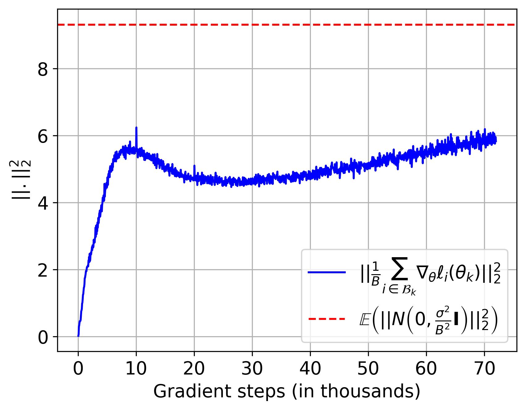
Figure 2: Noisy-SGD on ImageNet. We compare the norm of the mini-batch gradient to the one of the Gaussian noise when training with Noisy-SGD on ImageNet, for $B=128$ and the same set-up as in Figure 1. The noise magnitude is greater than the gradients.

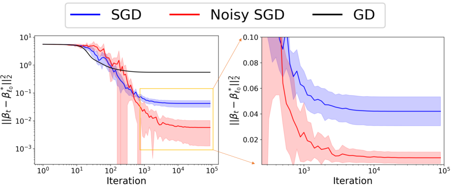
Figure 3: Diagonal Linear Network: Implicit Bias of GD, SGD and Noisy SGD ($\sigma=0.5$ in Equation 18). Shaded areas represent one standard deviation over 5 runs. (Left) Compared to GD with the same initialisation $\alpha=0.1$, SGD attain solutions closer to the sparse $\beta^{*}_{l_{0}}$, as expected from Pesme et al. (2021). Moreover, we observe that Noisy-SGD has a better implicit bias than SGD: the gradient noise structure is enhanced by perturbations. (Right) In absolute terms, Noisy-SGD does not even showcase more variance than SGD (near convergence).

3.2 Linear Least Square

The simplest model to study is Linear Least Square. We verify that noisy versions of SGD leads to similar solutions than SGD and GD.

Warm-up: Underparametrized setting ($n>d$)

The stochastic noise $\varepsilon(\theta)$ (cf. Equation 4) does not vanish near optimal solutions. For fixed $\epsilon>0$, we consider the following SDE as the continuous approximation of SGD (Ali et al., 2020):

$$d\theta_{t}=-\bar{X}^{T}(\bar{X}\theta_{t}-Y)dt+\sqrt{\gamma}\epsilon\bar{X}^{T}dW_{t}$$ (12)

We notice that it respects the characteristics highlighted in Section 2.2. This Orsnten-Uhlenbeck process has a limit, which can be solved through its characteristic Lyapunov equation (see Appendix A). With $X^{\dagger}$ the pseudo-inverse of $X$ and $\theta^{LS}:=X^{\dagger}Y$:

$$\theta_{\infty}\sim\mathcal{N}\left(\theta^{LS},\frac{\gamma\epsilon^{2}}{2}I_{d}\right)$$ (13)

We now consider adding isotropic Gaussian noise on top of the gradient’s structured noise of SGD:

$$d\theta_{t}=-\bar{X}^{T}(\bar{X}\theta_{t}-Y)dt+\sqrt{\gamma}\epsilon\bar{X}^{T}dW_{t}+\sigma d\tilde{W_{t}}$$ (14)

Solving the characteristic Lyapunov equation (see Appendix A), the limiting distribution becomes:

$$\boxed{\theta_{\infty}\sim\mathcal{N}\left(\theta^{LS},\frac{\gamma\epsilon^{2}}{2}I_{d}+\frac{\sigma^{2}}{4}(\bar{X}^{T}\bar{X})^{-1}\right)}$$ (15)

We observe that adding isotropic noise changes the limiting distribution: its shape depends on the training data. This simple example shows that geometry variation of the noise in the linear least square setting implies a controlled variation of the limiting process.

Over parametrized case ($d>n$):

As described in Section 2.2, GD and SGD will in this case both converge to $\theta^{LS}$ and therefore have the same implicit bias. SGD’s dynamic can be studied through the following SDE (Ali et al., 2020), where this time the gradient noise vanishes near the interpolators:

$$d\theta_{t}=-\bar{X}^{T}(\bar{X}\theta_{t}-Y)dt+\sqrt{\gamma}\|X\theta_{t}-Y\|_{2}\bar{X}^{T}dB_{t}$$ (16)

which also respects SGD’s specificities. $\theta_{t}$ converges to $\theta^{LS}$ for $\gamma\leq 1/Tr(\bar{X}^{T}\bar{X})$. If we add a constant spherical Gaussian noise at each step, the iterates will not converge. We thus look at the impact of adding a noise with a similar scale as the gradient noise:

$$\begin{split}d\beta_{t}&=-\bar{X}^{T}(\bar{X}\beta_{t}-Y)dt+\sqrt{\gamma}\|X\beta_{t}-Y\|_{2}\bar{X}^{T}dB_{t}\\ &+\sqrt{\gamma}\|X\beta_{t}-Y\|_{2}\sigma d\tilde{B}_{t}\end{split}$$

We show that we can control the difference between the SDE and the noisy SDE through $\eta_{t}=\|\theta_{t}-\beta_{t}\|_{2}^{2}$:

Theorem 1.

If $\gamma\leq 1/Tr(\bar{X}^{T}\bar{X})$ then

$$\boxed{\mathbf{E}(\eta_{t})\leq\gamma d\sigma^{2}\int_{0}^{t}L(\beta_{t})ds}$$ (17)

Proof.

Apply Itô’s formula to $\eta_{t}$, see Appendix A ∎

Here, we have highlighted that the variation from the original SDE will be contingent on factors such as dimension, step size, noise magnitude, and convergence rate. As a result, the solution obtained from a noisy variant of SGD may closely resemble that of traditional SGD, thus leading to a similar implicit bias. The extent of this similarity depends on the parameters used.

3.3 Noisy-SGD training of DLNs

For a 2-layer DLN sparse regression, SGD-induced noise steers the optimization dynamics towards advantageous regions that exhibit better generalization than GD (i.e., more sparse) Pesme et al. (2021). We investigate the impact of the addition of Gaussian noise.

Continuous model for Noisy-SGD

Adding constant Gaussian noise at each gradient step as in Equation 11 inevitably makes the process diverge for overparametrized DLNs. However, adding Gaussian noise with comparable magnitude to that of the gradients still allows to study the impact of geometry deformation, while maintaining a vanishing noise, enabling convergence. Pesme et al. (2021) have shown that the SGD update can be written $w_{t+1,\pm}=-\gamma\nabla_{w_{t,\pm}}L(w_{t})\pm\gamma[X^{T}\zeta_{i_{t}}(\beta_{t})]\mathbin{\leavevmode\hbox to6.28pt{\vbox to6.28pt{\text{[drawing]}}}}w_{t,\pm}$, where $\zeta_{i_{t}}$ is detailed in Appendix B. We thus consider the following noisy update:

$$\begin{split}w_{t+1,\pm}=&-\gamma\nabla_{w_{t,\pm}}L(w_{t})\pm\gamma[X^{T}\zeta_{i_{t}}(\beta_{t})]\mathbin{\leavevmode\hbox to6.28pt{\vbox to6.28pt{\text{[drawing]}}}}w_{t,\pm}\\ &\pm\gamma\sigma_{t}Z_{t,\pm}\mathbin{\leavevmode\hbox to6.28pt{\vbox to6.28pt{\text{[drawing]}}}}w_{t,\pm},\end{split}$$ (18)

with $Z_{t,\pm}\sim\mathcal{N}_{d}(0,1)$ and $\sigma_{t}\in\mathbb{R}^{\mathbb{R}}$. We consider here $\sigma_{t}=2\sigma\sqrt{L(w_{t})}$ for $\sigma\geq 0$, and show more general results in Appendix B. The corresponding SDE is:

$$\begin{split}dw_{t,\pm}=&\mp[\bar{X}^{T}r(w_{t})]\mathbin{\leavevmode\hbox to6.28pt{\vbox to6.28pt{\text{[drawing]}}}}w_{t,\pm}dt\\ &+2\sqrt{\gamma L(w_{t})}w_{t,\pm}\mathbin{\leavevmode\hbox to6.28pt{\vbox to6.28pt{\text{[drawing]}}}}\bar{X}^{T}dB_{t,\pm}\\ &+2\sigma\sqrt{\gamma L(w_{t})}w_{t,\pm}\mathbin{\leavevmode\hbox to6.28pt{\vbox to6.28pt{\text{[drawing]}}}}d\tilde{B}_{t,\pm}\end{split}$$ (19)

where $r(w)=\bar{X}(w^{2}_{+}-w^{2}_{-}-\beta^{\ast})$ and $\beta^{*}$ is an interpolator. We notice that compared to the SDE of Pesme et al. (2021), it only adds the term $2\sigma\sqrt{\gamma L(w_{t})}w_{t,\pm}\mathbin{\leavevmode\hbox to6.28pt{\vbox to6.28pt{\text{[drawing]}}}}d\tilde{B}_{t,\pm}$. See section 6 for a discussion on the impact of modeling with a decreasing noise, and appendix B for detailed computation of the link between equations (18) and (19).

We now demonstrate that despite the Gaussian perturbation, $\beta$ follows a stochastic mirror flow similar to the one in Pesme et al. (2021), detailed in Section 2.2:

Proposition 1.

Let $(w_{t,\pm})_{t\geq 0}$ be defined as in equation (19) from initialisation $\alpha$. Then $(\beta_{t}=w_{t,+}^{2}-w_{t,-}^{2})_{t\geq 0}$ follows a stochastic mirror flow defined by:

$$\begin{split}d\nabla\phi_{\alpha_{t}^{\beta}}(\beta_{t})=&-\nabla L(\beta_{t})dt+\sqrt{\gamma L(\beta_{t})}\bar{X}^{T}dB_{t}\\ &+\sqrt{\gamma L(\beta_{t})}\sigma d\tilde{B}_{t}\end{split}$$ (20)

where $\tilde{B}_{s}=(\tilde{B}_{s,+}+\tilde{B}_{s,+})/{2}$, $B_{s}=(B_{s,+}+B_{s,+})/{2}$,

$$\begin{split}\alpha^{\beta}_{t}=&\alpha\exp{(-2\gamma\sigma^{2}\int_{0}^{t}L(\beta_{s})ds)}\\ &\mathbin{\leavevmode\hbox to6.28pt{\vbox to6.28pt{\text{[drawing]}}}}\exp{(-2\gamma\mathrm{diag}(\bar{X}^{T}\bar{X})\int_{0}^{t}L(\beta_{s})ds)}\end{split}$$ (21)

Proof.

See appendix B. ∎

The continuous version of SGD analysed by Pesme et al. (2021) had led to the following mirror flow:

$$d\nabla\phi_{\alpha_{t}}(\beta_{t})=-\nabla L(\beta_{t})dt+\sqrt{\gamma L(\beta_{t})}\bar{X}^{T}dB_{t}$$ (22)

With $\alpha_{t}=\alpha\exp\left(-2\gamma\mathrm{diag}(\bar{X}^{T}\bar{X})\int_{0}^{t}L(\beta_{s})ds\right)$. Our resulting SDE for Noisy-SGD (cf. Equation 20) differs by two aspects: the additional spherical noise $\sqrt{\gamma L(\beta_{t})}\sigma d\tilde{B}_{t}$ and a smaller effective value for $\alpha$.

Solution.

If $\beta$ follows the original mirror flow, than the process converges with high probability towards $\operatorname*{arg\,min}_{\theta\text{ s.t. }X\theta=Y}\phi_{\alpha_{\infty}}$. This formulation is possible only because the KKT conditions are respected by the limit vector, as the updates remain confined to $\text{span}(x_{1},...,x_{n})$. However, this is no longer the case for Noisy-SGD. We still show a comparable outcome.

Theorem 2.

Let $(w_{t})_{t\geq 0}$ follow the SDE (19) from initialisation $\alpha$. Then for any $p$ close to $0$ there is a constant $C$ s.t. for any step size $\gamma\leq C$, with probability at least $1-p$, $\int_{0}^{\infty}\beta_{s}ds$ converges and $\beta_{t}$ converges with high probability to an interpolator $\beta_{\infty}$.

Proof.

We give here an idea of the proof which is along the lines of the proof found in Pesme et al. (2021). We first note that by arbitrarily changing $\bar{X}^{T}$ in SDE (22), the process still converges. In our case:

$$dw_{t,\pm}=-\nabla_{w_{\pm}}L(w_{t})dt+2\sqrt{\gamma L(w_{t})}w_{t,\pm}\mathbin{\leavevmode\hbox to6.28pt{\vbox to6.28pt{\text{[drawing]}}}}[AdB_{t,\pm}]$$

where this time $B_{t}$ is valued in $\mathbb{R}^{d+n}$ and $A:=\left(\bar{X}|\sigma I_{d}\right)$. The whole proof is given in Appendix B ∎

However, because the corresponding mirror flow updates no longer lie in $\text{span}(x_{1},...,x_{n})$ (cf. Equation 20), the KKT conditions of the minimization problem are no longer verified by $\beta_{\infty}$, and

$$\beta_{\infty}\neq\operatorname*{arg\,min}_{\beta\text{ s.t. }X\beta=Y}\phi_{\alpha^{\beta}_{\infty}}(\beta)$$ (23)

Nevertheless, we show that $\beta_{\infty}$ satisfy the KKT conditions for a small perturbation of that problem:

Proposition 2.

Under the assumptions of Theorem 2, on the set of convergence of $\beta_{t}$, there exists $r_{\infty}$ s.t.:

$$\boxed{\beta_{\infty}=\operatorname*{arg\,min}_{X\beta=Y}\phi_{\alpha_{\infty}}(\beta)-\langle r_{\infty},\beta\rangle}$$ (24)

Proof.

Let us consider $P$ the orthogonal projection over span$(x_{1},...,x_{n})$. Integrating (20) and decomposing the right hand side as a term $v\in$span$(x_{1},...,x_{n})$ and a term in the orthogonal, we get:

$$\nabla\phi_{\alpha_{\infty}}(\beta_{\infty})=v+\int_{0}^{\infty}\sigma\sqrt{\gamma L(\beta_{s})}(1-P)dBs$$ (25)

Let us define $r_{\infty}=\int_{0}^{\infty}\sigma\sqrt{\gamma L(\beta_{s})}(1-P)dBs$, and $\tilde{\beta}_{0}=\nabla\phi_{\alpha_{\infty}}^{-1}(r_{\infty})$, which is well defined by strong convexity of $\phi_{\alpha_{\infty}}$ (Refer to Appendix B). We have:

$$\nabla\phi_{\alpha_{\infty}}(\beta_{\infty})-\nabla\phi_{\alpha_{\infty}}(\tilde{\beta}_{0})\in\text{span}(x_{1},...,x_{n})$$ (26)

Thus, by defining $D$ the following Bregman divergence:

$$D_{\phi_{\alpha_{\infty}}}(\beta,\tilde{\beta}_{0})=\phi_{\alpha_{\infty}}(\beta)-\phi_{\alpha_{\infty}}(\tilde{\beta}_{0})-\langle\nabla\phi_{\alpha_{\infty}}(\tilde{\beta}_{0}),\beta-\tilde{\beta}_{0}\rangle$$

The gradient taken at $\beta_{\infty}$ lies in $\text{span}(x_{1},...,x_{n})$, insuring that the KKT conditions of the following problem are verified and thus:

$$\boxed{\beta_{\infty}=\operatorname*{arg\,min}_{X\beta=Y}D_{\phi_{\alpha_{\infty}}}(\beta,\tilde{\beta}_{0})}$$ (27)

∎

Therefore, Noisy-SGD gives the same solution as GD but on a different potential $\phi_{\alpha_{\infty}}$ and from an effective initialization $\tilde{\beta}_{0}$, while SGD only changes $\alpha$. For Noisy-SGD, we note that $\alpha_{\infty}$ decreases with $\sigma$ (eq. 21): the more noise is added, the smaller is the effective $\alpha$. If it did not change the effective initialization too, it would directly imply “better” implicit bias.

Implicit Bias

We have observed that $\beta_{\infty}$ is the solution to a perturbed minimization problem. We show now that the distance between $\beta_{\infty}$ and the optimizer of $\phi_{\alpha_{\infty}}$ can be controlled by the perturbation $\sigma$:

Proposition 3.

Under the assumptions of theorem 2 and on the high probability set of convergence of $(\beta_{t})$ let $\beta^{\ast}_{\alpha_{\infty}}:=\operatorname*{arg\,min}_{X\beta=Y}\phi_{\alpha_{\infty}}(\beta)$ and $r_{\infty}:=\sigma\int_{0}^{\infty}\sqrt{\gamma L(\beta_{s})}(1-P)dBs$. Since $\alpha_{\infty}>0$, $\phi_{\alpha_{\infty}}$ is $\mu$ strongly convex for $\mu>0$. Then we have:

$$\frac{1}{\mu}\|r_{\infty}\|_{2}\geq\|\beta^{\ast}_{\alpha_{\infty}}-\beta_{\infty}\|_{2}$$ (28)

Proof.

See Appendix B. ∎

We observe that although increasing $\sigma$ implies a lower $\alpha_{\infty}$ than SGD, which should yield to sparser solutions, it also implies a new effective initialization $\tilde{\beta}_{0}$ that deviates the solution from the sparse $\beta^{\ast}_{\alpha_{\infty}}$. However, in Figure 3, we show that Noisy-SGD still leads to sparser solutions than SGD. This might be attributed to the fact that the gain from a smaller $\alpha$ is in this case more important than the perturbation controlled by $\frac{1}{\mu}\|r_{\infty}\|\propto\sigma$, as shown in Figure 4. We give more details in the experiment section 4.2.

Proofs are derived in Appendix B.1 with more general noise forms, with stability results for the implicit bias.

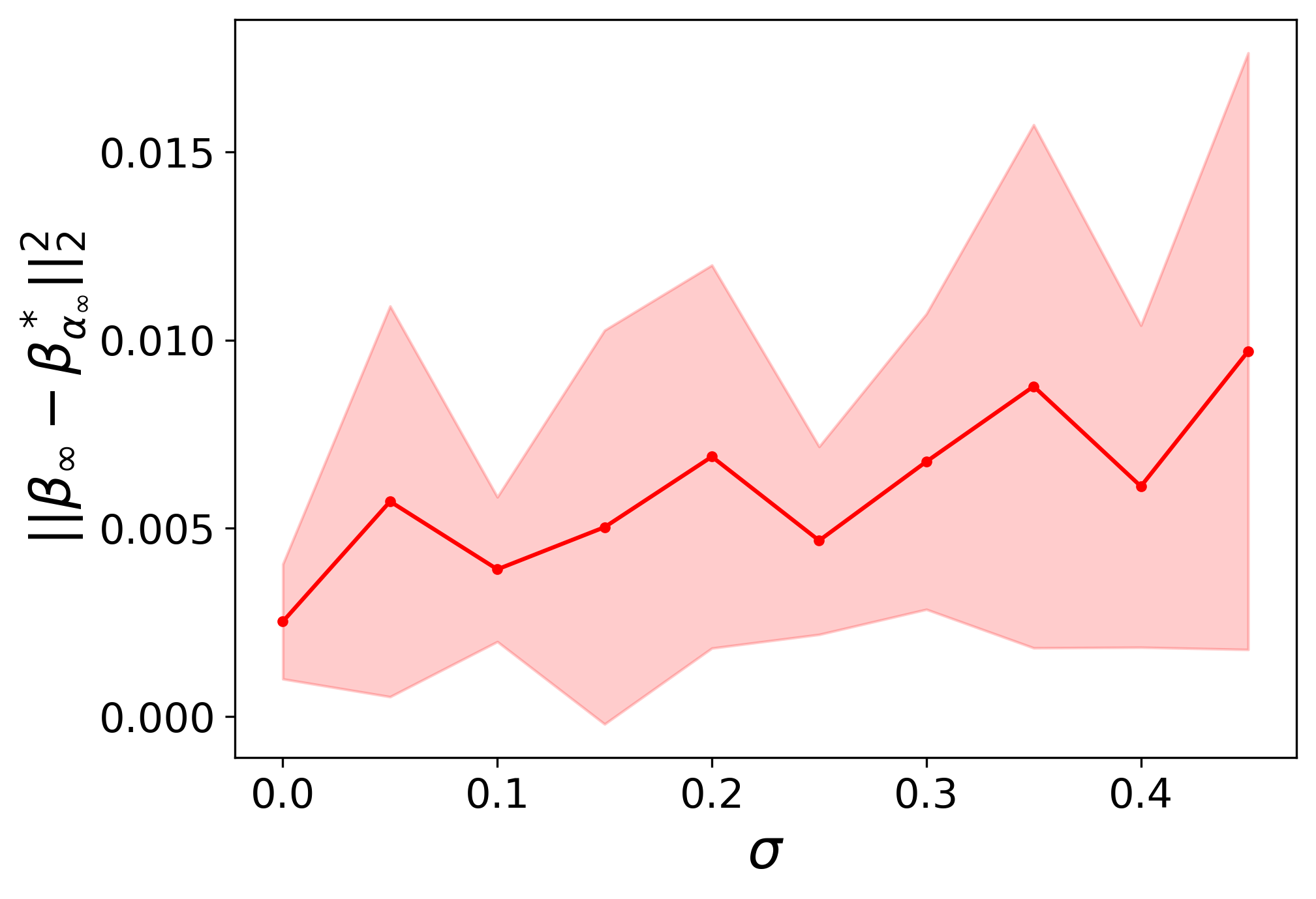
Figure 4: DLN: Distance between $\beta^{*}_{\alpha_{\infty}}$, the solution that minimizes $\phi_{\alpha_{\infty}}$ —obtained by GD from $\alpha_{\infty}$— and the one obtained by Noisy-SGD (see Proposition 3). Shaded areas represent one standard deviation over 10 runs. For small $\sigma$, the distance is smaller than the distance between the solutions of SGD and the sparse solution $\beta_{l_{0}}$ (see Figure 3), explaining why the implicit bias persists and can be enhanced by Gaussian noise.

4 Experiments

4.1 Noisy SGD on ImageNet

Dataset and architecture

To compare Noisy-SGD to DP-SGD, we adopt the exact same set-up as Sander et al. (2023). We train a Normalizer-Free ResNets (NF-ResNets) (Brock et al., 2021) with $d=25$M parameters on the ImageNet-1K dataset (Deng et al., 2009; Russakovsky et al., 2014) with blurred faces, which contains $1.2$ million images partitioned into 1000 categories. We use the timm (Wightman, 2019) library based on Pytorch (Paszke et al., 2019).

Optimization

For SGD and Noisy-SGD, we use a constant learning rate of $0.5$ and no momentum. We perform an exponential moving average of the weights (Tan and Le, 2019) with a decay parameter of $0.999$ (similar to Sander et al. (2023)). We set the effective noise $\sigma/B$ constant to $6\times 10^{-4}$ for all Noisy-SGD experiments of Figure 1, which is 4 times greater than the noise used by Sander et al. (2023) for ImageNet.

Implicit bias and Noise level

In Figure 2, we show that the additional Gaussian noise has a bigger $l_{2}$ norm than the gradients throughout training, for the same set-up as in Figure 1. It is an important observation because it shows that the additional Gaussian noise is not negligible, and thus that a similar implicit bias to the one of SGD persists even under strong Gaussian perturbation. Moreover, we notice that the training trajectories of SGD and Noisy-SGD do differ in Figure 1, especially at the beginning. However, the gradient norm $||\frac{1}{B}\sum_{i\in\mathcal{B}_{k}}\nabla_{\bm{\theta}}\ell_{i}(\bm{\theta}_{k})||$ increases during training, while the corresponding quantity in DP-SGD is bounded by 1 (cf. Equation 2 when $C=1$), which makes the actual signal-to-noise ratio greater in Noisy-SGD compared to DP-SGD.

4.2 Diagonal Linear Network

We adopt the same set-up as Pesme et al. (2021) for sparse regression. We select parameters n = 40 and d = 100, and then create a sparse model $\beta^{*}_{l_{0}}$ with the constraint that its $l_{0}$ norm is equal to 5. We generate the features $x_{i}$ from a normal distribution with mean 0 and identity covariance matrix $N(0,I)$, and compute the labels as $y_{i}=x_{i}^{T}\beta^{*}_{l_{0}}$. We always use the same step size of $\gamma=1/(1.3||\bar{X}\bar{X}^{T}||_{2})$. Notice that $||\beta_{t}-\beta^{*}_{l_{0}}||^{2}_{2}$ is the validation loss in the experiments.

Noisy-SGD’s improved implicit Bias

In Figure 3, we show that noisy-SGD produces sparser solutions than the one obtaimed with SGD, as it is closer to the sparse interpolator $\beta_{l_{0}}$. This effect is primarily due to the impact of having a smaller effective value $\alpha$ which outweighs the impact of the perturbation governed by the new effective initialization $\tilde{\beta_{0}}$: $\frac{1}{\mu}\|r_{\infty}\|\propto\sigma$ (see Equation 3). In Appendix B.2, we also illustrate scenarios where the parameter $\sigma$ becomes more prominent in comparison to $\alpha$, and for which Noisy-SGD still induce a stronger implicit bias.

Impact of $\sigma$

In Figure 4, we run Noisy-SGD for different values of $\sigma$, $10$ times for each value, and show the averages and standard deviations. As expected from Proposition 3, the distance between $\beta^{*}_{\alpha_{\infty}}$, the actual minimizer under constraints of $\phi_{\alpha_{\infty}}$ and $\beta_{\infty}$, the solution obtained from Noisy-SGD, increases with $\sigma$. We observe that the order of magnitude of this increase, which was hidden inside the constants of the Proposition, is reasonable when compared to the distance between the solution of SGD and the sparse interpolator, as depicted in Figure 3. It explains why using $\sigma=0.5$ still helps when starting from $\alpha=0.1$.

5 Conclusion

The challenge of achieving strong performance in large-batch DP-SGD training remains a critical obstacle in balancing privacy and utility. This performance bottleneck in DP-SGD is poised to become more pronounced over time as the theoretical solution to further bridging the performance gap between private and non-private training lies in the expansion of both training set size and batch size (Sander et al., 2023).

We have observed that Noisy-SGD exhibits a performance decline with the batch size, indicating that the gradient noise in SGD still plays a pivotal role, even with Gaussian perturbation. It puts in perspective a key argument supporting that the inherent geometry of SGD’s noise is responsible for its bias. For DLNs, a seemingly minor addition of Gaussian noise disrupts a crucial KKT condition, necessitating a complex mathematical alternative. We’ve derived proofs for broader noise in Appendix B.1 and offer stability results that extend the amplification of the implicit bias. Overall, our study underscores two critical points:

• The specific gradient noise geometry in SGD is robust to Gaussian perturbations, and different geometries can lead to different implicit biases

• Further work could try to leverage methods developed to improve large-batch training in non-private settings (e.g., employing the LARS optimizer (You et al., 2017) for convolutional DNNs) to enhance the performance of DP-SGD, thus advancing the trade-off between privacy and utility.

6 Discussion

Our decision to study Noisy-SGD as a substitute for DP-SGD is primarily based on the observations depicted in figure 1. Notably, a similar implicit bias of DP-SGD is discernible even in the absence of clipping. We delve here into the implications of using Noisy-SGD as a stand-in DP-SGD. This includes considerations from both optimization and privacy perspectives.

An optimization perspective.

Noisy-SGD only aligns with DP-SGD if the gradients are bounded, an assumption that is commonly done in convergence studies (Bassily et al., 2014). This is not the case for classical neural networks, nor for the DLN case that we studied. Without any assumption, the clipping operation can bias the (expected) direction of the update. However, assuming symmetricity of the gradients, which is a reasonable assumption (Chen et al., 2020), the drift maintains its direction after clipping.

If we take clipping into account for DLNs while assuming symetricity, the noise term can still be approximated by $\sigma_{t}\circ w_{t}dB_{t}$, where $\sigma_{t}$ now depends on $w_{t}$. Indeed, if we denote $y_{t}:=\langle\beta-\beta^{\ast},x_{i_{t}}\rangle x_{i_{t}}$, we get $w_{t+1}=w_{t}-\gamma\mathbb{E}[\text{clip}(y_{t}\circ w_{t})]-\gamma(\text{clip}(y_{t}\circ w_{t})-\mathbb{E}[\text{clip}(y_{t}\circ w_{t})])$. The mean zero term rewrites as $\alpha(y_{t},w_{t})y_{t}\circ w_{t}-\mathbb{E}[\alpha(y_{t},w_{t})y_{t}\circ w_{t}]$, with first order of the covariance$(1/n)\text{diag}(w_{t})\alpha^{2}\mathbb{E}[y_{t}y_{t}^{T}]\text{diag}(w_{t})$. Our extension in appendix B.1 is a first approximation.

A privacy perspective.

We deliberately focus on the sole effect of noise addition and its impact on the optimization procedure. Nevertheless, we do theoretically show how the noise level impacts our results, with additional experiments presented in Appendix B.2, and general forms in appendix B.1. However, vanishing noise would always lead to exploding privacy guarantees. We use this modelisation as a first approximation, as it changes the structure of the noise similarly to DP. Moreover, it is necessary for convergence as the learning is constant; studying a decreasing learning rate with fixed noise could have been an alternative, but we should have taken a different angle (unknown) to study the bias. In a similar vein, one could consider the clipping component more comprehensively. One potential approach could be to proportionally decrease the clipping value in tandem with the noise magnitude. This method would not only uphold the privacy guarantees but also ensure convergence

Appendix A Linear Least Square

We detail the proofs of the Propositions presented in Section 3.2 focusing on the continuous analysis of the implicit bias of SGD and Noisy-SGD in the Linear Least Square Setting. We start with the under parametrized case in Section A.1 where the number of parameters $d$ is smaller than the number of training data points $n$. Subsequently, we delve into the over parameterized case in Section A.2.

A.1 Under Parameterized Case

SDE for SGD

In situations where the model is underparameterized, the gradient noise encompasses the entire space of $\mathbb{R}^{d}$ and there is a specific value of $\epsilon>0$ such that $||X\theta_{t}-Y||$ remains greater than $\epsilon$ for all time steps $t$, as documented in Ali et al. (2020). We thus consider the following SDE as the continuous approximation of SGD in the linear least square under parametrized setting. In this framework, the Euler discretization with a step size of $\gamma$ corresponds to the implementation of SGD, incorporating the noise modelization previously described:

$$d\theta_{t}=-\bar{X}^{T}(\bar{X}\theta_{t}-Y)dt+\sqrt{\gamma}\epsilon\bar{X}^{T}dW_{t}$$ (29)

This process is a Orsnten-Uhlenbeck process that can be written as:

$$d\theta_{t}=\beta(\mu-\theta_{t})dt+\Sigma dW_{t}$$ (30)

with $\mu=(X^{T}X)^{-1}X^{T}Y=X^{\dagger}Y:=\theta^{LS}$ for $X^{\dagger}$ the pseudo-inverse of $X$, $\beta=\bar{X}^{T}\bar{X}$ and $\Sigma=\sqrt{\gamma}\epsilon\bar{X}^{T}$.

The stationary distribution of this temporally homogeneous Markov Chain is:

$$\theta_{\infty}=\mathcal{N}(\theta^{LS},w)$$ (31)

for $w$ that verifies the following Lyapunov equation:

$$\beta w+w\beta^{T}=2D=\gamma\epsilon^{2}\beta$$ (32)

For $D=\Sigma^{T}\Sigma/2=\frac{\gamma\epsilon^{2}}{2}\beta$. The solution of this Lyapunov equation can be directly solved as:

$$w=\int_{0}^{\infty}e^{-t\beta}(-2D)e^{-t\beta}\,dt=\int_{0}^{\infty}e^{-t\beta}(-\gamma\epsilon^{2}\beta)e^{-t\beta}\,dt=-\gamma\epsilon^{2}\beta\int_{0}^{\infty}e^{-2t\beta}\,dt=\frac{\gamma\epsilon^{2}}{2}I_{d}$$ (33)

As $\int_{0}^{\infty}e^{-2t\beta}\,dt=\beta^{-1}/2$. The commutativity results from the fact that all matrices are sums of powers of $\beta$ within the integrals.

Noisy-SDE

Let us now consider adding Gaussian noise to the modelisation of the natural SGD noise:

$$d\theta_{t}=-\bar{X}^{T}(\bar{X}\theta_{t}-Y)dt+\sqrt{\gamma}\epsilon\bar{X}^{T}dW_{t}+\sigma d\tilde{W_{t}}$$ (34)

we get the same equations for $\Sigma=(\sqrt{\gamma}\epsilon\bar{X}^{T}|\sigma I_{d})\in\mathbf{R}^{d\times(n+d)}$ and $W=(W^{T}|\tilde{W}^{T})^{T}$.

So $D=\frac{\Sigma\Sigma^{T}}{2}=\frac{\frac{\gamma}{n}\epsilon^{2}X^{T}X+\sigma^{2}I_{d}}{2}=\frac{\gamma\epsilon^{2}}{2}\beta+\frac{\sigma^{2}}{2}I_{d}$, and in this case:

$$w=\int_{0}^{\infty}e^{-t\beta}(-\gamma\epsilon^{2}\beta)e^{-t\beta}\,dt-\frac{\sigma^{2}}{2}(-\frac{1}{2}\beta^{-1})=\frac{\gamma\epsilon^{2}}{2}I_{d}+\frac{\sigma^{2}}{4}\beta^{-1}$$ (35)

With $\beta^{-1}=(\bar{X}^{T}\bar{X})^{-1}$. Finally:

$$\boxed{\theta_{\infty}\sim\mathcal{N}\left(\theta^{LS},\frac{\gamma\epsilon^{2}}{2}I_{d}+\frac{\sigma^{2}}{4}(\bar{X}^{T}\bar{X})^{-1}\right)}$$ (36)

In this case, we observe that adding spherical noise adds a dependence on the data distribution to the variance term.

A.2 Over Parameterized Case

In the overparametrised regime, the noise vanishes at every global optimum $\theta^{\star}$, and is degenerate in the directions of $\text{Ker}(X)$, giving the following continuous approximation (Pillaud-Vivien and Pesm, 2022; Ali et al., 2020):

$$d\theta_{t}=-\bar{X}^{T}(\bar{X}\theta_{t}-Y)dt+\sqrt{\gamma}\|X\theta_{t}-Y\|_{2}\bar{X}^{T}dB_{t}$$ (37)

In this case, $\theta_{t}$ converges almost surely to $\theta^{LS}$ for $\gamma>0$ and $\theta_{0}=0$. Let us now consider the following noisy version of SGD, with an additional noise that has the same magnitude as the gradient noise:

$$\begin{split}d\beta_{t}&=-\bar{X}^{T}(\bar{X}\beta_{t}-Y)dt+\sqrt{\gamma}\|X\beta_{t}-Y\|_{2}\bar{X}^{T}dB_{t}\\ &+\sqrt{\gamma}\|X\beta_{t}-Y\|_{2}\sigma d\tilde{B}_{t}\end{split}$$

We show that we can control the difference between the iterates of the first SDE and its noisy version: $\eta_{t}=\|\theta_{t}-\beta_{t}\|_{2}^{2}$. More precisely,

If $\gamma\leq 2/Tr(\bar{X}^{T}\bar{X})$ then

$$\boxed{\mathbf{E}(\eta_{t})\leq\gamma d\sigma^{2}\int_{0}^{t}L(\beta_{t})ds}$$

Proof.

We can write $d\beta_{t}=-\bar{X}^{T}(\bar{X}\beta_{t}-Y)dt+\sqrt{\gamma}\|X\beta_{t}-Y\|_{2}(\bar{X}^{T}|\sigma I_{d})dB^{\prime}_{t}$ for $B^{\prime}=(\frac{B}{\tilde{B}})\in\mathbb{R}^{n+d}$. Similarly to $\theta$, for $\beta_{0}=0$ and $\gamma>0$, $\beta$ converges almost surely. So $\theta-\beta$ converges and finally $\eta$ converges. Applying Itô’s formula, we get:

$$\begin{split}d\eta_{t}&=[-2\|\bar{X}(\theta_{t}-\beta_{t})\|^{2}\\ &+\gamma Tr(\bar{X}^{T}\bar{X})(\sqrt{R_{n}(\theta_{t})}-\sqrt{R_{n}(\beta_{t})})^{2}\\ &+d\sigma^{2}\gamma R_{n}(\beta_{t})]dt+...dW_{t}+...d\tilde{W}_{t}\end{split}$$

Straightforwardly using the triangular inequality, we have:

$$(\sqrt{R_{n}(\theta_{t})}-\sqrt{R_{n}(\beta_{t})})^{2}\leq||\bar{X}(\theta_{t}-\beta_{t})||^{2}_{2}=||\bar{X}\theta_{t}-Y-(\bar{X}\beta_{t}-Y)||^{2}_{2}\leq(\sqrt{R_{n}(\theta_{t})}+\sqrt{R_{n}(\beta_{t})})^{2}$$ (38)

Looking now at the expected value, the Brownian motions disappear and injecting Inequality 38:

$$\begin{split}\mathbb{E}(\eta_{t})&=\gamma d\sigma^{2}\int_{0}^{t}R_{n}(\beta_{s})ds-2\int_{0}^{t}\|\bar{X}(\theta_{s}-\beta_{s})\|_{2}^{2}ds+\gamma Tr(\bar{X}^{T}\bar{X})\int_{0}^{t}(\sqrt{R_{n}(\theta_{s})}-\sqrt{R_{n}(\beta_{s})})^{2}\\ &\leq\gamma d\sigma^{2}\int_{0}^{t}R_{n}(\beta_{t})ds+(\gamma Tr(\bar{X}^{T}\bar{X})-2)\int_{0}^{t}\|\bar{X}(\theta_{s}-\beta_{s})\|^{2}ds\end{split}$$

Finally, for $\gamma<2/Tr(\bar{X}^{T}\bar{X})$,

$$\boxed{\mathbf{E}(\eta_{t})\leq\gamma d\sigma^{2}\int_{0}^{t}R_{n}(\beta_{s})ds=\gamma d\sigma^{2}\int_{0}^{t}L(\beta_{s})ds}$$

and in particular,

$$\boxed{\mathbf{E}(\eta_{\infty})\leq\gamma d\sigma^{2}\int_{0}^{\infty}L(\beta_{s})ds}$$

∎

Appendix B Diagonal Linear Network

In this Section, we first derive in Section B.1 the mathematical proofs of the Propositions and Theorems presented in Section 3.3. We then show more empirical results on the sparsity of the solutions obtained with Noisy-SGD, when training a DLN.

B.1 Mathematical proofs

B.1.1 Modelisation

Recall that the weights $(w_{t,\pm})_{t\geq 0}$ are defined through the following SDE

$$dw_{t,\pm}=\pm[\bar{X}^{T}r(w_{t})]\mathbin{\leavevmode\hbox to6.28pt{\vbox to6.28pt{\text{[drawing]}}}}w_{t,\pm}dt+2\sqrt{\gamma L(w_{t})}w_{t,\pm}\mathbin{\leavevmode\hbox to6.28pt{\vbox to6.28pt{\text{[drawing]}}}}\bar{X}^{T}dB_{t,\pm}+2\sigma\sqrt{\gamma L(w_{t})}w_{t,\pm}\mathbin{\leavevmode\hbox to6.28pt{\vbox to6.28pt{\text{[drawing]}}}}d\tilde{B}_{t,\pm}$$

The Euler discretization of that SDE with step size $\gamma$ is exactly

$$w_{t+1,\pm}=w_{t,\pm}-\gamma\nabla_{w_{t,\pm}}L(w_{t})\pm 2\sqrt{\gamma L(w_{t})}[\bar{X}^{T}\epsilon]\mathbin{\leavevmode\hbox to6.28pt{\vbox to6.28pt{\text{[drawing]}}}}w_{t,\pm}\pm\gamma\sigma_{t}Z_{t,\pm}\mathbin{\leavevmode\hbox to6.28pt{\vbox to6.28pt{\text{[drawing]}}}}w_{t,\pm},$$

Where $\epsilon\sim\mathcal{N}(0,\sqrt{\gamma}Id)$. As seen in (Pesme et al., 2021, Appendix A) the covariance of $2\sqrt{nL(w_{t})}\frac{1}{\sqrt{\gamma}}\epsilon$ is equal to the one of $\zeta_{i_{t}}$. Where

$$\zeta_{i_{t}}=-\left(\langle\beta-\beta^{\ast},x_{i_{t}}\rangle e_{i_{t}}-\mathbb{E}_{i_{t}}[\langle\beta-\beta^{\ast},x_{i_{t}}\rangle e_{i_{t}}]\right)$$

with $i_{t}$ the random index chosen for the step of SGD. Thus the discretization scheme defines a Markov-Chain whose noise is the one found in equation (18) (the other term being independant from the rest).

B.1.2 Proof of Proposition 1

This section and the following one essentially adapt the proof of a similar result found in Pesme et al. (2021) in order to generalize it to more complex noise pattern. In particular extend it to a noise which does not depend on the loss and thus the geometry of the gradients. We consider throughout this section a more general setting. Let $A\in\mathbb{R}^{p\times d}$ which in the main text is either equal to $\bar{X}$ and thus $p=n$ or to $\left(\bar{X}\mid\sigma I_{d}\right)$ and $p=d+n$. And let a covariance noise matrix $(\sigma_{t})$ which is deterministic and valued in $\mathbb{R}^{p^{\prime}\times d}$. Set $(w_{t,\pm})$ solutions of the following SDE with $w_{0,\pm}=\alpha$.

$$\begin{split}dw_{t,\pm}&=-\nabla_{w_{\pm}}L(\beta_{t})dt\pm 2\sqrt{\gamma L(\beta_{t})}w_{t,\pm}\mathbin{\leavevmode\hbox to6.28pt{\vbox to6.28pt{\text{[drawing]}}}}\left[A^{T}dB_{t}\right]\pm 2w_{t,\pm}\mathbin{\leavevmode\hbox to6.28pt{\vbox to6.28pt{\text{[drawing]}}}}\left[\sigma_{t}^{T}d\tilde{B}_{t}\right]\\ &=\pm\left(-\bar{X}^{T}r(\beta_{t})\mathbin{\leavevmode\hbox to6.28pt{\vbox to6.28pt{\text{[drawing]}}}}w_{t,\pm}dt+2\sqrt{\gamma L(\beta_{t})}w_{t,\pm}\mathbin{\leavevmode\hbox to6.28pt{\vbox to6.28pt{\text{[drawing]}}}}\left[A^{T}dB_{t}\right]+2w_{t,\pm}\mathbin{\leavevmode\hbox to6.28pt{\vbox to6.28pt{\text{[drawing]}}}}\left[\sigma_{t}^{T}d\tilde{B}_{t}\right]\right)\end{split}$$

where $r(w)=\bar{X}(w_{+}^{2}-w_{-}^{2}-\beta^{\ast})$ and $(B_{t})_{t},(\tilde{B}_{t})_{t}$ are two independant standard brownian motions respectively valued in $\mathbb{R}^{p}$ and $\mathbb{R}^{p^{\prime}}$. This setting accounts for a decaying noise which has a geometry different to the one of the data as well a as a small noise which is solely of the magnitude of the parameters.

Lemma 1.

Consider the iterates $(w_{t})$ defined above (9) then $(\beta_{t}=w_{t,+}^{2}-w_{t,-}^{2})$ satisfies

$$\beta_{t}=2\alpha_{t}^{2}\text{sinh}(2\eta_{t}+2\delta_{t})$$

where

$$\eta_{t}=-\int_{0}^{t}\bar{X}^{T}r(w_{s})ds+2\sqrt{\gamma}\int_{0}^{t}\sqrt{L(w_{s})}A^{T}dB_{s},\quad\delta_{t}=2\int_{0}^{t}\sigma_{s}^{T}d\tilde{B}_{s}$$

and

$$\alpha_{t}=\alpha\mathbin{\leavevmode\hbox to6.28pt{\vbox to6.28pt{\text{[drawing]}}}}\exp\left(-2\gamma\text{diag}(A^{T}A)\int_{0}^{t}L(\beta_{s})ds-2\int_{0}^{t}\text{diag}(\sigma_{t}^{T}\sigma_{t})ds\right)$$

Proof.

A direct application of Itô’s lemma grants

$$\begin{split}w_{t,\pm}&=w_{0,\pm}\mathbin{\leavevmode\hbox to6.28pt{\vbox to6.28pt{\text{[drawing]}}}}\exp(\pm\left[-\int_{0}^{t}\bar{X}^{T}r(w_{s})ds+2\sqrt{\gamma}\int_{0}^{t}\sqrt{L(w_{s})}A^{T}dB_{s}+2\int_{0}^{t}\sigma_{s}^{T}d\tilde{B}_{s}\right])\\ &\mathbin{\leavevmode\hbox to6.28pt{\vbox to6.28pt{\text{[drawing]}}}}\exp(-2\gamma\text{diag}(A^{T}A)\int_{0}^{t}L(\beta_{s})ds-2\int_{0}^{t}\text{diag}(\sigma_{t}^{T}\sigma_{t})ds)\end{split}$$

Thus since $\beta_{t}=w_{t,+}^{2}-w_{t,-}^{2}$ we have

$$\begin{split}\beta_{t}&=\alpha_{t}^{2}\mathbin{\leavevmode\hbox to6.28pt{\vbox to6.28pt{\text{[drawing]}}}}(\exp(+2\eta_{t}+2\delta_{t})-\exp(-2\eta_{t}-2\delta_{t}))\\ &=2\alpha_{t}^{2}\text{sinh}(2\eta_{t}+2\delta_{t})\end{split}$$

∎

The next result is the generalization of the result introducing the notion of mirror gradient descent with varying potential found in (Pesme et al., 2021, Proposition 1).

Proposition 4.

The flow $(\beta_{t})_{t\geq 0}$ associated to $(w_{t,\pm})_{t\geq 0}$ follows a stochastic mirror gradient with varying potential defined by:

$$d\nabla\phi_{\alpha_{t}}(\beta_{t})=-\nabla L(\beta_{t})dt+\sqrt{\gamma L(\beta_{t})}A^{T}dB_{t}+\sigma_{t}^{T}d\tilde{B}_{t}$$

Proof.

The expression of $\beta_{t}$ from lemma 1 can be inversed in order to use $\phi_{\alpha_{t}}$. Indeed

$$\text{arcsinh}\left(\frac{\beta_{t}}{2\alpha_{t}^{2}}\right)=2\eta_{t}+2\delta_{t}$$

which implies

$$d\text{arcsinh}\left(\frac{\beta_{t}}{2\alpha_{t}^{2}}\right)=-2\bar{X}^{T}r(w_{t})+4\sqrt{\gamma L(\beta_{t})}A^{T}dB_{t}+4\sigma_{t}^{T}d\tilde{B}_{t}$$

Notice that $\nabla L(\beta_{t})=\frac{1}{2}\bar{X}^{T}r(w_{t})$ and $\nabla\phi_{\alpha}(\beta)=\frac{1}{4}\text{arcsinh}(\frac{\beta}{2\alpha^{2}})$ we have the wanted result. ∎

B.1.3 Proof of Theorem 2

In order to prove the convergence of the integral of the loss we will introduce a perturbation of a Bregman divergence which will control the norm of the iterates and the integral of the loss. Moreover that process will be nicely controlled with high probability. Let $\beta^{\ast}$ any interpolator, the process is the following

$$\begin{split}V_{t}&=-\phi_{\alpha_{t}}(\beta_{t})+\langle\nabla\phi_{\alpha_{t}}(\beta_{t}),\beta_{t}-\beta^{\ast}\rangle\\ &+\langle|\beta^{\ast}|,\gamma\text{diag}(A^{T}A)\int_{0}^{t}L(\beta_{s})ds+\int_{0}^{t}\text{diag}(\sigma_{s}^{T}\sigma_{s})ds\rangle\end{split}$$

We denote by $D_{t}$ the Bregman divergence part.

Lemma 2.

For $t\geq 0$ we have

$$\begin{split}dD_{t}&=-2L(\beta_{t})+\gamma L(\beta_{t})\langle\xi_{t},\text{diag}(A^{T}A)\rangle dt+\langle\xi_{t},\text{diag}(\sigma_{t}^{T}\sigma_{t})\rangle dt\\ &+\sqrt{\gamma L(\beta_{t})}\langle A^{T}dB_{t},\beta_{t}-\beta^{\ast}\rangle+\langle\sigma_{t}^{T}d\tilde{B}_{t},\beta_{t}-\beta^{\ast}\rangle\end{split}$$

where $\xi_{t}=\sqrt{\beta_{t}^{2}+4\alpha_{t}^{4}}=w_{t,+}^{2}+w_{t,-}^{2}$

Proof.

By definition $D_{t}=-\phi_{\alpha_{t}}(\beta_{t})+\langle\nabla\phi_{\alpha_{t}}(\beta_{t}),\beta_{t}-\beta^{\ast}\rangle$ thus a direct application of Itô’s lemma grants

$$\begin{split}dD_{t}&=-\langle\nabla\phi_{\alpha_{t}}(\beta_{t}),d\beta_{t}\rangle-\langle\nabla_{\alpha}\phi(\alpha_{t}^{2},\beta),d[\alpha_{t}^{2}]\rangle-\frac{1}{2}\text{Tr}\left(\nabla^{2}\phi_{\alpha_{t}}(\beta_{t})d\langle\beta\rangle_{t}\right)\\ &+\langle d\nabla\phi_{\alpha_{t}}(\beta_{t}),\beta_{t}-\beta^{\ast}\rangle+\langle\nabla\phi_{\alpha_{t}}(\beta_{t}),d\beta_{t}\rangle+\text{Tr}\left(d\langle\nabla\phi_{\alpha_{t}}(\beta_{t}),\beta_{t}\rangle\right)\\ &=-\langle\nabla_{\alpha}\phi(\alpha_{t}^{2},\beta),d[\alpha_{t}^{2}]\rangle-\frac{1}{2}\text{Tr}\left(\nabla^{2}\phi_{\alpha_{t}}(\beta_{t})d\langle\beta\rangle_{t}\right)+\langle d\nabla\phi_{\alpha_{t}}(\beta_{t}),\beta_{t}-\beta^{\ast}\rangle\\ &+\text{Tr}\left(d\langle\nabla\phi_{\alpha_{t}}(\beta_{t}),\beta_{t}\rangle\right)\end{split}$$

We will compute one by one the four terms left. Note that todo so we will need to compute the quadratic variation of $\beta_{t}$. Since $\beta_{t}$ can be decomposed in a drift part and a martingale part as follows

$$d\beta_{t}=\text{drift}(\beta)_{t}dt+4\sqrt{\gamma L(\beta_{t})}\xi_{t}\mathbin{\leavevmode\hbox to6.28pt{\vbox to6.28pt{\text{[drawing]}}}}A^{T}dB_{t}+4\xi_{t}\mathbin{\leavevmode\hbox to6.28pt{\vbox to6.28pt{\text{[drawing]}}}}\sigma_{t}^{T}d\tilde{B}_{t}$$

we obtain this formula for the quadratic variation

$$d\langle\beta\rangle_{t}=16\gamma L(\beta_{t})(A^{T}A)\mathbin{\leavevmode\hbox to6.28pt{\vbox to6.28pt{\text{[drawing]}}}}(\xi_{t}\xi_{t}^{T})+16(\sigma_{t}^{T}\sigma_{t})\mathbin{\leavevmode\hbox to6.28pt{\vbox to6.28pt{\text{[drawing]}}}}(\xi_{t}\xi^{T}_{t})$$

Since $\alpha_{t}$ has no martingale part the chain rule grants that the first term is equal to

$$\langle\nabla_{\alpha}\phi(\alpha_{t}^{2},\beta),d[\alpha_{t}^{2}]\rangle=\gamma L(\beta_{t})\langle\xi_{t},\text{diag}(A^{T}A)\rangle dt+\langle\xi_{t},\text{diag}(\sigma_{t}^{T}\sigma_{t})\rangle dt$$

Since $\nabla^{2}\phi_{\alpha}(\beta)=\frac{1}{4}\text{diag}(\frac{1}{\xi})$ the second term is equal to

$$\frac{1}{2}\text{Tr}\left(\nabla^{2}\phi_{\alpha_{t}}(\beta_{t})d\langle\beta\rangle_{t}\right)=2\gamma L(\beta_{t})\langle\xi_{t},\text{diag}(A^{T}A)\rangle dt+2\langle\xi_{t},\gamma\text{diag}(\sigma_{t}^{T}\sigma_{t})\rangle dt$$

Using proposition 4 the third term is equal to

$$\langle d\nabla\phi_{\alpha_{t}}(\beta_{t}),\beta_{t}-\beta^{\ast}\rangle=-\langle\nabla L(\beta_{t}),\beta_{t}-\beta^{\ast}\rangle+\sqrt{\gamma L(\beta_{t})}\langle A^{T}dB_{t},\beta_{t}-\beta^{\ast}\rangle+\langle\sigma_{t}^{T}d\tilde{B}_{t},\beta_{t}-\beta^{\ast}\rangle$$

the fourth term

$$\text{Tr}\left(d\langle\nabla\phi_{\alpha_{t}}(\beta_{t}),\beta_{t}\rangle\right)=4\gamma L(\beta_{t})\langle\xi_{t},\text{diag}(A^{T}A)\rangle dt+4\langle\xi_{t},\gamma\text{diag}(\sigma_{t}^{T}\sigma_{t})\rangle dt$$

Note that

$$\langle\nabla L(\beta_{t}),\beta_{t}-\beta^{\ast}\rangle=2L(\beta_{t})$$

Thus combined it grants

$$\begin{split}dD_{t}&=-2L(\beta_{t})+\gamma L(\beta_{t})\langle\xi_{t},\text{diag}(A^{T}A)\rangle dt+\langle\xi_{t},\text{diag}(\sigma_{t}^{T}\sigma_{t})\rangle dt\\ &+\sqrt{\gamma L(\beta_{t})}\langle A^{T}dB_{t},\beta_{t}-\beta^{\ast}\rangle+\langle\sigma_{t}^{T}d\tilde{B}_{t},\beta_{t}-\beta^{\ast}\rangle\end{split}$$

∎

The Bregman divergence is useful to control the iterations as the next lemma will state. Moreover under suitable assumptions on the noise $\sigma_{t}$ the martingale part being close to its quadratic variation will enable us to control $V_{t}$ itself and in turns the loss.

Lemma 3.

For $t\geq 0$ we have

$$\|\xi_{t}\|_{1}\leq 4V_{t}+\|\beta^{\ast}\|_{1}\ln\left(\frac{\sqrt{2}\|\xi_{t}\|_{1}}{\min\alpha_{i}^{2}}\right)$$

Proof.

A direct computation grants

$$\|\xi_{t}\|_{1}=4D_{t}+\langle\text{arcsinh}\frac{\beta_{t}}{4\alpha_{t}^{2}},\beta^{\ast}\rangle$$ (39)

Since $\text{arcsinh(x)}\leq\ln(2(x+1))$ we have

$$\begin{split}\langle\text{arcsinh}\frac{\beta_{t}}{4\alpha_{t}^{2}},\beta^{\ast}\rangle&\leq\sum_{i}|\beta^{\ast}_{i}|\ln\left(\frac{|\beta_{i,t}|+2\alpha_{i,t}^{2}}{\alpha_{i,t}^{2}}\right)\\ &\leq\sum_{i}|\beta^{\ast}_{i}|\ln\left(\frac{|\beta_{i,t}|+2\alpha_{i,t}^{2}}{\min\alpha_{i}^{2}}\right)+4\langle|\beta^{\ast}|,\gamma\text{diag}(A^{T}A)\int_{0}^{t}L(\beta_{s})ds+\int_{0}^{t}\text{diag}(\sigma_{s}^{T}\sigma_{s})ds\rangle\\ &\leq\|\beta^{\ast}\|_{1}\ln\left(\frac{\sqrt{2}\|\xi_{t}\|_{1}}{\min\alpha_{i}^{2}}\right)+4\langle|\beta^{\ast}|,\gamma\text{diag}(A^{T}A)\int_{0}^{t}L(\beta_{s})ds+\int_{0}^{t}\text{diag}(\sigma_{s}^{T}\sigma_{s})ds\rangle\end{split}$$

Because $\alpha_{t}^{2}=\alpha^{2}\mathbin{\leavevmode\hbox to6.28pt{\vbox to6.28pt{\text{[drawing]}}}}\exp\left(-4\gamma\text{diag}(A^{T}A)\int_{0}^{t}L(\beta_{s})ds-4\int_{0}^{t}\text{diag}(\sigma_{s}^{T}\sigma_{s})ds\right)$ and $|\beta_{i,t}|+2\alpha_{i,t}^{2}\leq\sqrt{2}\|\xi_{t}\|_{1}$. Thus plugging that inequation in the first relationship (39) grants the wanted result. ∎

We now need to control $V_{t}$, however in order to only have to manage bounded variation processes we will use the fact that a Martingale is controlled by its quadratic variation

Lemma 4 (Howard et al. (2020), Corollary 11).

For any locally square integrable process $(S_{t})$ with a.s. continuous trajectories and any $a,b>0$

$$\mathbb{P}(\exists t\geq 0,S_{t}\geq a+b\langle S\rangle_{t})\leq\exp(-2ab)$$

We can use this lemma for the following two processes

$$\int_{0}^{t}\sqrt{\gamma L(\beta_{s})}\langle A^{T}dB_{s},\beta_{s}-\beta^{\ast}\rangle,\quad\int_{0}^{t}\langle\sigma_{s}^{T}d\tilde{B}_{s},\beta_{s}-\beta^{\ast}\rangle$$

For $a,b>0$ we have thanks to lemma 4 with probability at least $1-2\exp(-ab)$ for any $t\geq 0$

$$\begin{split}&\left|\int_{0}^{t}\sqrt{\gamma L(\beta_{s})}\langle A^{T}dB_{s},\beta_{s}-\beta^{\ast}\rangle+\langle\sigma_{s}^{T}d\tilde{B}_{s},\beta_{s}-\beta^{\ast}\rangle\right|\\ &\leq a+b\gamma\|A\|^{2}\int_{0}^{t}L(\beta_{s})(\|\beta_{s}\|^{2}+\|\beta^{\ast}\|^{2})ds+b\int_{0}^{t}\|\sigma_{s}\|^{2}(\|\beta_{s}\|^{2}+\|\beta^{\ast}\|^{2})ds\end{split}$$

because the quadratic variation of both processes are upperbounded by the term on the right. We denote by $\mathcal{A}$ the set on which the inequality above is satsfied, we recall that this set has probability at least $1-2\exp(-ab)$.

Lemma 5.

On $\mathcal{A}$ for $\gamma$ and $\int\|\sigma_{s}\|^{2}ds$ small enough the iterates are bounded by a constant that only depends on $a,b,\|\beta^{\ast}\|,\alpha$.

Proof.

Since we are on the event $\mathcal{A}$ the bound on the martingale part is true and thus

$$V_{t}\leq V_{0}+a-2\int_{0}^{t}L(\beta_{s})U_{s}ds+\int_{0}^{t}\langle|\beta^{\ast}|,\text{diag}(\sigma_{s}^{T}\sigma_{s})\rangle+b\|\sigma_{s}\|^{2}(\|\beta_{s}\|^{2}+\|\beta^{\ast}\|^{2})ds$$

Where $U_{s}=1-\frac{\gamma}{2}\left[\langle\text{diag}(A^{T}A,\xi_{s}+|\beta^{\ast}|\rangle+2b\|A\|^{2}(\|\beta_{s}\|^{2}+\|\beta^{\ast}\|^{2})ds)\right]$. Assume that $\int_{0}^{\infty}\|\sigma_{s}\|^{2}ds\leq 1$, then we have

$$V_{t}\leq C-2\int_{0}^{t}L(\beta_{s})U_{s}ds+\int_{0}^{t}C^{\prime}\|\sigma_{s}\|^{2}\|\beta_{s}\|^{2}ds$$

Where $C$ depends on $a,b,\|\beta^{\ast}\|_{1}$ and $V_{0}$ which depends on $\alpha$ also $C^{\prime}$ depends on $b$. In particular if $U_{s}\geq 0$ for $s\in[0,\tau]$ using lemma 3 we have for other constants $C,C^{\prime}$ and $t\in[0,\tau]$

$$\|\xi_{t}\|_{1}\leq\|\beta^{\ast}\|_{1}\ln\left(\frac{\sqrt{2}\|\xi_{t}\|_{1}}{\min\alpha_{i}^{2}}\right)+C+\int_{0}^{t}C^{\prime}\|\sigma_{s}\|\|\beta_{s}\|^{2}ds$$

Since $\|\beta_{s}\|^{2}\leq\|\xi_{s}\|^{2}$ and by the sublinear growth of the log we get

$$\|\xi_{t}\|_{2}\leq C+\int_{0}^{t}C^{\prime}\|\sigma_{s}\|^{2}\|\xi_{s}\|^{2}ds$$

For another set of constants $C,C^{\prime}$. We now use a bootstrap argument let $I=\{t\in[0,\tau]\mid\forall s\leq t,\|\xi_{t}\|_{2}\leq 2C\}$. Assume that $\int_{0}^{\infty}\|\sigma_{s}\|^{2}ds\leq 1/4CC^{\prime}$ then $I=[0,\tau]$. Indeed $0\in I$ and $I$ is an interval. Let $t=\sup I$, first $t\in I$ and if $t=\tau$ there is nothing to prove. If $t<\tau$ then

$$\frac{\|\xi_{t}\|_{2}}{2C}\leq\frac{1}{2}+\int_{0}^{t}2CC^{\prime}\|\sigma_{s}\|^{2}\left(\frac{\|\xi_{s}\|_{2}}{2C}\right)^{2}ds\leq\frac{1}{2}+\int_{0}^{t}2CC^{\prime}\|\sigma_{s}^{2}\|ds<1$$

And by continuity of $\xi$ we have $t+\epsilon\in I$. Thus $I=[0,\tau]$ and for any $t\in[0,\tau]$ we have that $\xi$ is bounded by a constant which only depends on the parameters of the problem. Now we shall see that for a nice choice of $\gamma$ we have $\tau=+\infty$ on $\mathcal{A}$. Indeed for $\gamma$ small enough we have $U_{0}\geq 1/2$. Now let $t$ the waiting time for $U$ to reach $1/2$. Then by continuity of $U$ for $s\leq t$ we have $U_{s}\geq 1/2>0$ thus the bound on the iterates found above is valid and for $\gamma$ small enough we have that $U_{t}>1/2$ which is a contradiction by continuity of $U$. Thus there is a threshold under which $U$ is always greater than $1/2$. Thus the above bound on the iterates is valid for all times. ∎

Proposition 5.

On $\mathcal{A}$ for $\gamma$ and $\int\|\sigma_{s}\|^{2}ds$ small enough the integral of the loss converges.

Proof.

In the proof of the last lemma we have shown that for the right choice of $\gamma$ and $\int\|\sigma_{s}\|^{2}ds$, $U_{s}$ is greater than $\frac{1}{2}$ on $\mathcal{A}$. Thus by boundedness of the iterates we have

$$\int_{0}^{t}L(\beta_{s})ds\leq C-V_{t}+C^{\prime}\int_{0}^{t}\|\sigma_{s}\|^{2}ds$$

It remains to lower bound $V$ in order to prove convergence of the integral of the loss. Or the computations in lemma 3 shows that

$$V_{t}\geq\frac{1}{4}\left(\|\xi_{t}\|_{1}-\|\beta^{\ast}\|_{1}\ln\left(\frac{\sqrt{2}\|\xi_{t}\|_{1}}{\min\alpha_{i}^{2}}\right)\right)$$

which is lower bounded because the iterates are bounded. Thus the integral converges. ∎

Finally we have all the ingredients to show that the iterates converge.

Proposition 6.

On $\mathcal{A}$ for $\gamma$ and $\int\|\sigma_{s}\|^{2}ds$ small enough the iterates converge.

Proof.

We have the following integral expression of $D_{t}$ thanks to lemma 2

$$\begin{split}D_{t}&=D_{0}+\int_{0}^{t}-2L(\beta_{s})+\gamma L(\beta_{s})\langle\xi_{s},\text{diag}(A^{T}A)\rangle+\langle\xi_{s},\text{diag}(\sigma_{s}^{T}\sigma_{s})\rangle ds\\ &+\int_{0}^{t}\sqrt{\gamma L(\beta_{s})}\langle\bar{X}^{T}dB_{s},\beta_{s}-\beta^{\ast}\rangle+\langle\sigma_{s}d\tilde{B}_{s},\beta_{s}-\beta^{\ast}\rangle ds\end{split}$$

Note that $D_{t}$ converges because the bouded variation part converges due to the convergence of the integral of the loss and the boundedness of the iterates. The martingale part converges because the quadratic variation is converging. Recall that

$$D_{t}=-\phi_{\alpha_{t}}+\langle\nabla\phi_{\alpha_{t}}(\beta_{t}),\beta_{t}-\beta^{\ast}\rangle$$

We have that $D$ converges for any choice of interpolator $\beta^{\ast}$.
The integral of the loss is convergent thus up to extraction $L(\beta_{t})$ converges to 0. Since $\beta_{t}$ is bounded a second extraction ensures the converges of the iterates. Thus there is a subsequence $\beta_{\psi(t)}$ such that it converges to $\beta_{\infty}$ and $L(\beta_{\infty})=0$ thus it is an interpolator. And we have

$$\begin{split}\phi_{\alpha_{\infty}}(\beta_{\infty})-D_{t}&=\phi_{\alpha_{\infty}}(\beta_{\infty})-\phi_{\alpha_{t}}(\beta_{t})-\langle\nabla\phi_{\alpha_{t}}(\beta_{t}),\beta_{t}-\beta_{\infty}\rangle\\ &\geq\phi_{\alpha_{t}}(\beta_{\infty})-\phi_{\alpha_{t}}(\beta_{t})-\langle\nabla\phi_{\alpha_{t}}(\beta_{t}),\beta_{t}-\beta_{\infty}\rangle\\ &=D_{\phi_{\alpha_{t}}}(\beta_{\infty},\beta)\\ &\geq 0\end{split}$$

Because $\alpha\mapsto\phi_{\alpha}(\beta)$ is decreasing and $\alpha_{t}\geq\alpha_{\infty}$. Note that $\phi_{\alpha_{\infty}}(\beta_{\infty})-D_{\psi(t)}\to 0$ by convergence of $\beta_{\psi(t)}$ to $\beta_{\infty}$. Thus by convergence of $D$ we have that $\phi_{\alpha_{\infty}}(\beta_{\infty})-D_{t}\to 0$ and in turn $D_{\phi_{\alpha_{t}}}(\beta_{\infty},\beta)\to 0$. Recall that

$$\nabla^{2}\phi_{\alpha}(\beta)=\frac{1}{4}\text{diag}\left(\frac{1}{\sqrt{\beta^{2}+4\alpha^{2}}}\right)\geq\frac{1}{4\sqrt{\|\beta\|^{2}+4\max\alpha_{i}^{2}}}Id$$

thus $\phi_{\alpha_{t}}$ is strongly convex of with a parameter that does not depend on $t$ by decreasingness of $\alpha_{t}$ and boundedness of $\beta_{t}$. Thus we have that $D_{\phi_{\alpha_{t}}}(\beta_{\infty},\beta)\geq\mu/2\|\beta_{t}-\beta_{\infty}\|^{2}$ which concludes the convergence. ∎

B.1.4 Proof of Proposition 3

In the last section we have shown that the iterates converge toward an interpolator. However that interpolator is not a minimizer of the potential $\phi_{\alpha_{\infty}}$ as shown in proposition 2. However by strong convexity of $\phi_{\alpha}$ we have a control of the distance between $\beta_{\infty}$ and the minimizer of $\phi_{\alpha_{\infty}}$ which we denote by $\beta^{\ast}_{\alpha_{\infty}}$

Proof.

Let $\phi(\beta)=\phi_{\alpha_{\infty}}(\beta)+\iota_{X\beta=Y}$ where $\iota$ is the indicator function equal to $0$ if the condition is satisfied and $+\infty$ otherwise. Note that $\phi$ is still strongly convex. Indeed, we can show that $\phi-\mu\|.\|^{2}$ is convex: let $\beta,\nu\in\mathbb{R}^{d}$, $\lambda\in(0,1)$. $C=\{\beta\text{ s.t. }X\beta=Y\}$ is a convex set as an affine subspace of $\mathbb{R}^{d}$. Therefore:

$$\lambda\beta+(1-\lambda)\nu\notin C\implies\beta\notin C\text{ or }\nu\notin C$$ (40)

$$\iota_{X(\lambda\beta+(1-\lambda)\nu)=Y}=\infty\implies\iota_{X\beta=Y}=\infty\text{ or }\iota_{X\nu=Y}=\infty$$ (41)

We also have that $\phi_{\alpha_{\infty}}-\mu\|.\|^{2}$ is convex on a bounded set which contains $\beta_{\infty}$ and $\beta_{\alpha_{\infty}}^{\ast}$. Finally $\phi-\mu\|.\|^{2}$ is convex, i.e. $\phi$ is $\mu-$strongly convex on a bounded set.

We have $\beta_{\infty}$ solution of

$$\min\phi(\beta)-\langle r_{\infty},\beta\rangle$$ (42)

And $\beta_{\alpha_{\infty}}^{\ast}$ is the solution to

$$\min\phi(\beta)$$ (43)

Since $\phi$ is strongly convex we have that $f=\phi-\mu\|\cdot-\beta^{\ast}\|^{2}$ is convex. Notice that $0\in\partial f(\beta_{\infty})-r_{\infty}$ thus

$$\phi(\beta^{\ast})-\langle r_{\infty},\beta_{0}\rangle-\mu\|\beta^{\ast}-\beta_{\infty}\|^{2}\geq\phi(\beta_{\infty})-\langle r_{\infty},\beta_{\infty}\rangle$$ (44)

We thus observe that:

$$\phi(\beta^{\ast})-\langle r_{\infty},\beta^{\ast}\rangle\geq\phi(\beta_{\infty})-\langle r_{\infty},\beta_{\infty}\rangle+\mu\|\beta^{\ast}-\beta_{\infty}\|^{2}$$ (45)

Thus by optimality of $\beta^{\ast}$ ($\phi(\beta^{\ast})-\phi(\beta_{\infty})\leq 0$)

$$\begin{split}\langle r_{\infty},\beta_{\infty}-\beta^{\ast}\rangle&\geq\phi(\beta^{\ast})-\langle r_{\infty},\beta^{\ast}\rangle-(\phi(\beta_{\infty})-\langle r_{\infty},\beta_{\infty}\rangle)\\ &\geq\mu\|\beta^{\ast}-\beta_{\infty}\|^{2}\end{split}$$ (46)

Finally using Cauchy-Schwarz inequality we have

$$\boxed{\|r_{\infty}\|\geq\mu\|\beta^{\ast}-\beta_{\infty}\|}$$ (47)

∎

B.2 Additional Numerical Experiments

Reminder

We adopt the same set-up as Pesme et al. (2021) for sparse regression. We select parameters n = 40 and d = 100, and then create a sparse model $\beta^{*}_{l_{0}}$ with the constraint that its $l_{0}$ norm is equal to 5. We generate the features $x_{i}$ from a normal distribution with mean 0 and identity covariance matrix $N(0,I)$, and compute the labels as $y_{i}=x_{i}^{T}\beta^{*}_{l_{0}}$. We always use the same step size of $\gamma=1/(1.3||\bar{X}^{T}\bar{X}||_{2})$. Notice that $||\beta_{t}-\beta^{*}_{l_{0}}||^{2}_{2}$ is the validation loss in the experiments.

Introduction

As outlined in Section 3.3 and prooved in Section B.1 in a more general setting, our investigation reveals that Noisy-SGD yields an identical solution to GD, albeit (1) operating on an altered potential $\phi_{\alpha_{\infty}}$, and (2) starting from an effective non-zero initialization denoted as $\tilde{\beta}_{0}$. In contrast, the sole parameter affected by SGD is $\alpha$. In the context of Noisy-SGD, it is noteworthy that $\alpha_{\infty}$ diminishes with increasing $\sigma$. This signifies that as more noise is introduced, the effective $\alpha$ becomes smaller. If this did not influence the effective initialization, it would directly imply an “improved” implicit bias, in the case of the sparse regression under study.

Trade off

To be more precise, if the effective initialization $\tilde{\beta_{0}}$ remained unaltered, the noisy process would ultimately converge to $\beta^{\star}_{\alpha_{\infty}}$, which is the solution that minimizes $\phi_{\alpha_{\infty}}$. We already know that this solution is sparser than the one obtained via SGD because $\alpha_{\infty}$ is smaller (as referenced in Equation 21). As demonstrated in Proposition 3, the presence of the new effective initialization $\tilde{\beta_{0}}$ does introduce some perturbation to the solution. However, the degree of its influence directly depends on the level of noise introduced. This ensures that $\beta_{\infty}$, which is the solution obtained through Noisy-SGD, remains in close proximity to $\beta^{\star}_{\alpha_{\infty}}$. This scenario implies the existence of a tradeoff. Increasing the value of $\sigma$ will:

1. Augment the sparsity of $\beta^{\star}_{\alpha_{\infty}}$ as $\beta^{\star}_{\alpha_{\infty}}$ gets closer to the (sparse) ground truth $\beta^{\star}_{l_{0}}$

2. Expand the gap between $\beta_{\infty}$ and $\beta^{\star}_{\alpha_{\infty}}$, which could potentially diminish the impact of the first outcome if $\beta_{\infty}$ gets far from $\beta^{\star}_{l_{0}}$

In summary, if the influence of 1. surpasses the effect of 2., Noisy-SGD would enhance the implicit bias. Conversely, if 2. outweighs 1., this enhancement may not necessarily occur. To empirically quantify the trade-off, we measure the gap between $\beta^{\star}_{\alpha_{\infty}}$ and $\beta_{\infty}$ across varying values of $\alpha$ and $\sigma$. Our approach involves (a) obtaining $\beta_{\infty}$ through Noisy-SGD, (b) approximating $\alpha_{\infty}$ numerically based on the loss logs, and (c) subsequently executing GD with $\alpha=\alpha_{\infty}$ to obtain $\beta^{\star}_{\alpha_{\infty}}$. In Figure 4, our findings underscore that, for $\alpha=0.1$, the distance between $\beta^{\star}_{\alpha_{\infty}}$ and $\beta_{\infty}$ seem to indeed increase with growing values of $\sigma$, validating the second point (2.). Moreover, as revealed in Figure 3, when using $\alpha=0.1$, Noisy-SGD consistently converges to sparser solutions compared to standard SGD. This trend remains consistent across various noise levels, as illustrated in Figure 5. Specifically, as we elevate the magnitude of $\sigma$, the solutions become progressively closer to the sparse interpolator (ground truth). In this context, the influence of the new initialization $\tilde{\beta_{0}}$ appears to be of secondary importance, with therefore point 1. consistently holding more significance than point 2.

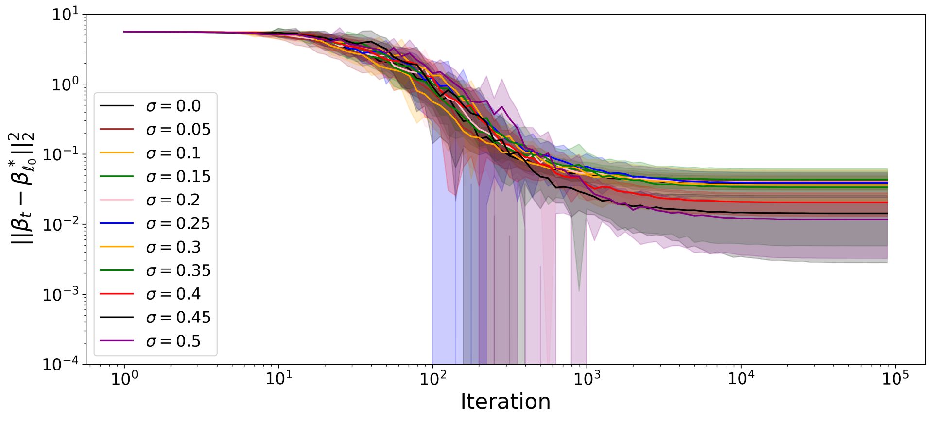
Figure 5: Diagonal Linear Network from $\alpha=0.1$: Implicit Bias of SGD and Noisy SGD different values of $\sigma$ in Equation 18, from $\alpha=0.1$. Shaded areas represent one standard variation over 5 runs, and plain lines represent the average values. Starting from this initialization, the bigger $\sigma$ is, the closer the solution obtained with Noisy-SGD is to the sparse solution $\beta^{*}_{l_{0}}$.

Nonetheless, Figure 4 reveals that the magnitude of the gap between $\beta^{\star}_{\alpha_{\infty}}$ and $\beta_{\infty}$ is smaller or comparable to the gap between $\beta_{\infty}$ and $\beta^{\star}_{l_{0}}$ in Figure 3. This observation implies that Noisy-SGD may be advantageous only in this specific scenario, as the impact of 2. is small. However, a question arises: if the initial $\alpha$ were even smaller, would 1. still dominate 2.?

Figure 6 provides insight into this inquiry. Even with an initial $\alpha$ reduced by a factor of ten, we observe that the introduction of noise continues to exert a positive influence on the sparsity of the solution. Furthermore, when examining the gap between $\beta^{\star}_{\alpha_{\infty}}$ and $\beta_{\infty}$ in Figure 7, we find that, similarly to the case where $\alpha=0.1$, it remains of a comparable order of magnitude to the gap between $\beta_{\infty}$ and $\beta^{\star}_{l_{0}}$ observed in Figure 6. This observation helps to elucidate why the advantages of Noisy-SGD persist under these conditions: the distance between $\beta^{\star}_{\alpha_{\infty}}$ and $\beta_{\infty}$ empirically also depends (inversely) on $\alpha$, which mitigates the impact of 2. over 1.

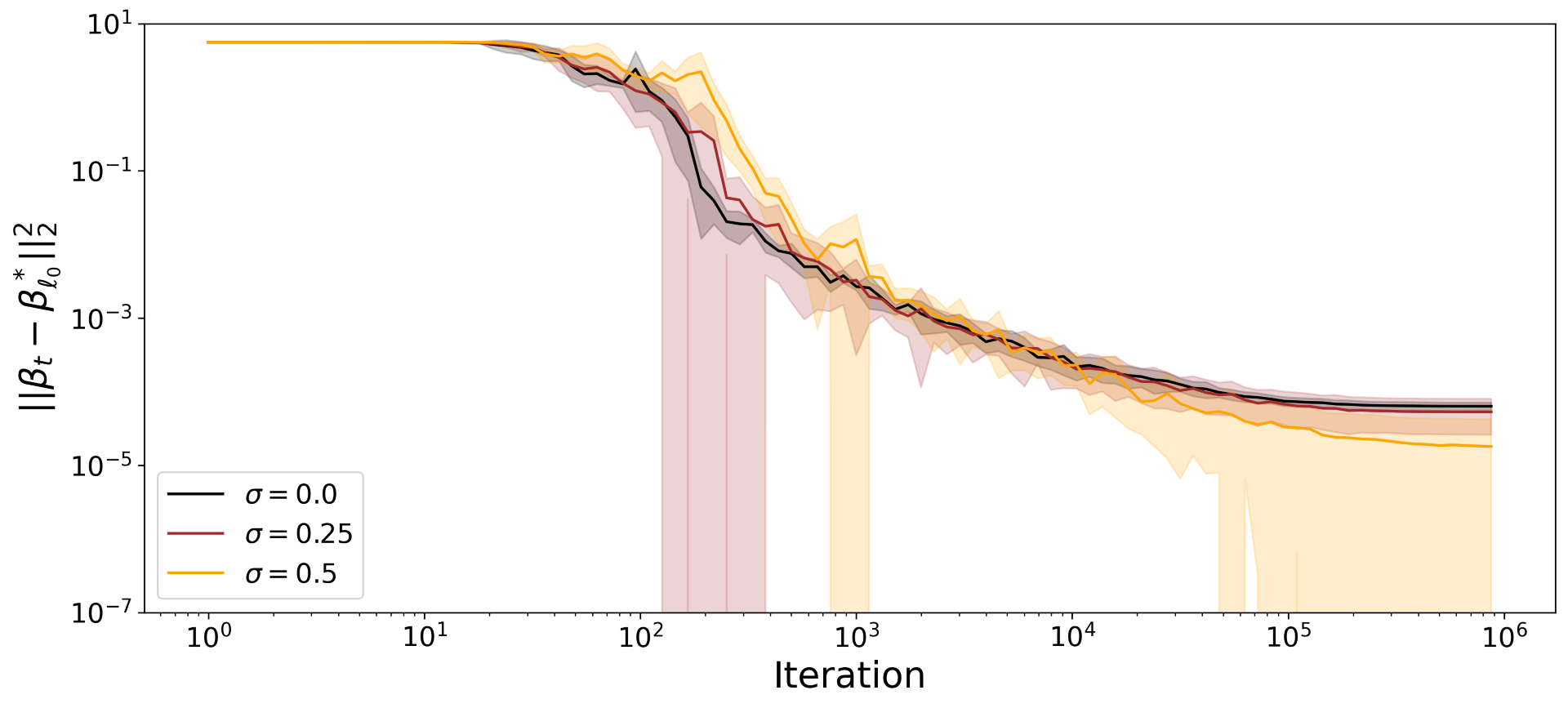
Figure 6: Diagonal Linear Network from $\alpha=0.01$: Implicit Bias of SGD and Noisy SGD different values of $\sigma$ in Equation 18, from small initialization $\alpha=0.01$. Shaded areas represent one standard variation over 5 runs, and plain lines represent the average values. Starting from this initialization, the bigger $\sigma$ is, the closer the solution obtained with Noisy-SGD is to the sparse solution $\beta^{*}_{l_{0}}$.

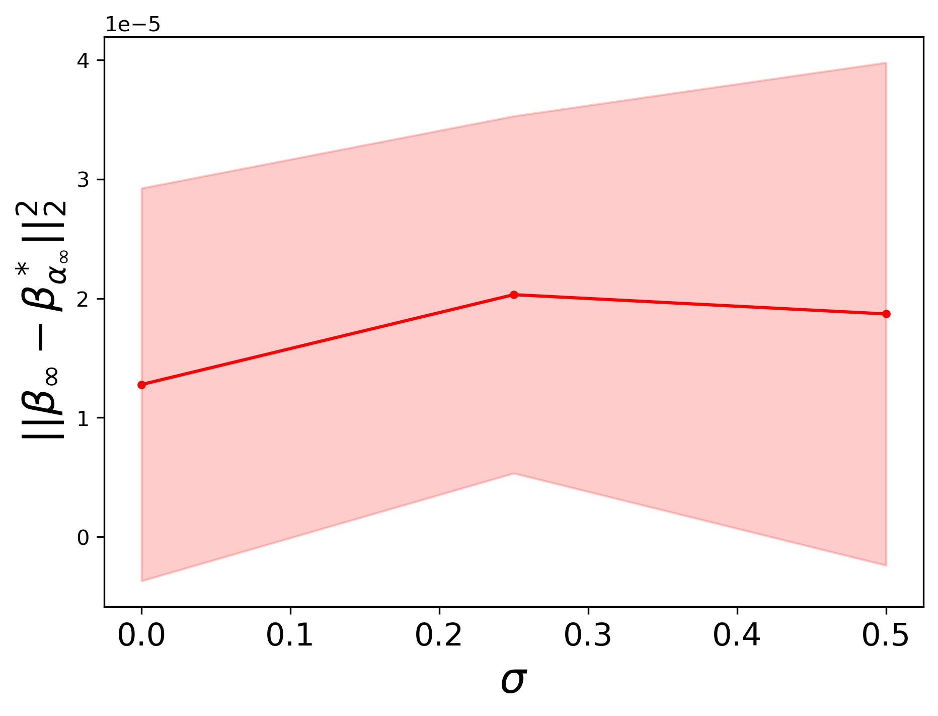
Figure 7: DLN from $\alpha=0.1$: Distance between $\beta^{*}_{\alpha_{\infty}}$, the solution that minimizes $\phi_{\alpha_{\infty}}$ —obtained by GD from $\alpha_{\infty}$— and $\beta_{\infty}$, the one obtained by Noisy-SGD from $\alpha=0.01$ (see Proposition 3). Shaded areas represent one standard deviation over 5 runs. Similar to the case of $\alpha=0.1$ (see Figure 4), the distance is of the same order of magnitude than the distance between $\beta_{\infty}$ and the sparse solution $\beta_{l_{0}}$ (see Figure 6). It explains why why the implicit bias is enhanced by Gaussian noise in this case.

Conclusion:

The effect of Noisy-SGD on the solution’s sparsity, as discussed in Section 3.3, remains significant even when initiated with smaller values of $\alpha$, which corresponds to cases where the solutions obtained from GD and SGD already exhibit some enhanced degree of sparsity. Therefore, the practical implications of the theoretical trade off appears to be modest, and the reinforcement of the implicit bias from Noisy-SGD prevails: the introduction of Gaussian noise enhances or at least maintains the implicit bias of SGD in a robust way.

References

- Sander et al. (2023) Tom Sander, Pierre Stock, and Alexandre Sablayrolles. Tan without a burn: Scaling laws of dp-sgd. In International Conference on Machine Learning, pages 29937–29949. PMLR, 2023.
- Robbins and Monro (1951) Herbert Robbins and Sutton Monro. A Stochastic Approximation Method. The Annals of Mathematical Statistics, 22(3):400 – 407, 1951. doi: 10.1214/aoms/1177729586. URL https://doi.org/10.1214/aoms/1177729586.
- Duflo (1996) M. Duflo. Algorithmes stochastiques. Mathématiques et Applications. Springer Berlin Heidelberg, 1996. ISBN 9783540606994. URL https://books.google.co.uk/books?id=ffkzAAAACAAJ.
- He et al. (2016) Kaiming He, Xiangyu Zhang, Shaoqing Ren, and Jian Sun. Deep residual learning for image recognition. In Proceedings of the IEEE conference on computer vision and pattern recognition, pages 770–778, 2016.
- Devlin et al. (2018) Jacob Devlin, Ming-Wei Chang, Kenton Lee, and Kristina Toutanova. Bert: Pre-training of deep bidirectional transformers for language understanding. arXiv preprint arXiv:1810.04805, 2018.
- Touvron et al. (2023) Hugo Touvron, Thibaut Lavril, Gautier Izacard, Xavier Martinet, Marie-Anne Lachaux, Timothée Lacroix, Baptiste Rozière, Naman Goyal, Eric Hambro, Faisal Azhar, et al. Llama: Open and efficient foundation language models. arXiv preprint arXiv:2302.13971, 2023.
- Amodei et al. (2016) Dario Amodei, Sundaram Ananthanarayanan, Rishita Anubhai, Jingliang Bai, Eric Battenberg, Carl Case, Jared Casper, Bryan Catanzaro, Qiang Cheng, Guoliang Chen, et al. Deep speech 2: End-to-end speech recognition in english and mandarin. In International conference on machine learning, pages 173–182. PMLR, 2016.
- Keskar et al. (2016) Nitish Shirish Keskar, Dheevatsa Mudigere, Jorge Nocedal, Mikhail Smelyanskiy, and Ping Tak Peter Tang. On large-batch training for deep learning: Generalization gap and sharp minima. arXiv preprint arXiv:1609.04836, 2016.
- Smith et al. (2020) Samuel L. Smith, Erich Elsen, and Soham De. On the generalization benefit of noise in stochastic gradient descent. CoRR, abs/2006.15081, 2020. URL https://arxiv.org/abs/2006.15081.
- Masters and Luschi (2018) Dominic Masters and Carlo Luschi. Revisiting small batch training for deep neural networks. arXiv preprint arXiv:1804.07612, 2018.
- HaoChen et al. (2020) Jeff Z. HaoChen, Colin Wei, Jason D. Lee, and Tengyu Ma. Shape matters: Understanding the implicit bias of the noise covariance, 2020.
- Carlini et al. (2019) Nicholas Carlini, Chang Liu, Úlfar Erlingsson, Jernej Kos, and Dawn Song. The secret sharer: Evaluating and testing unintended memorization in neural networks. In 28th USENIX Security Symposium, pages 267–284, 2019.
- Carlini et al. (2021) Nicholas Carlini, Florian Tramer, Eric Wallace, Matthew Jagielski, Ariel Herbert-Voss, Katherine Lee, Adam Roberts, Tom Brown, Dawn Song, Ulfar Erlingsson, et al. Extracting training data from large language models. In 30th USENIX Security Symposium (USENIX Security 21), pages 2633–2650, 2021.
- Dwork et al. (2006) Cynthia Dwork, Frank McSherry, Kobbi Nissim, and Adam Smith. Calibrating noise to sensitivity in private data analysis. In Proceedings of the Third Conference on Theory of Cryptography, page 265–284, 2006.
- Abadi et al. (2016) Martin Abadi, Andy Chu, Ian Goodfellow, H Brendan McMahan, Ilya Mironov, Kunal Talwar, and Li Zhang. Deep learning with differential privacy. In Proceedings of the 2016 ACM SIGSAC conference on computer and communications security, pages 308–318, 2016.
- Yu et al. (2021) Da Yu, Huishuai Zhang, Wei Chen, Jian Yin, and Tie-Yan Liu. Large scale private learning via low-rank reparametrization. In International Conference on Machine Learning, pages 12208–12218. PMLR, 2021.
- De et al. (2022) Soham De, Leonard Berrada, Jamie Hayes, Samuel L. Smith, and Borja Balle. Unlocking high-accuracy differentially private image classification through scale, 2022. URL https://arxiv.org/abs/2204.13650.
- Yu et al. (2023) Yaodong Yu, Maziar Sanjabi, Yi Ma, Kamalika Chaudhuri, and Chuan Guo. Vip: A differentially private foundation model for computer vision. arXiv preprint arXiv:2306.08842, 2023.
- Balle et al. (2022) Borja Balle, Giovanni Cherubin, and Jamie Hayes. Reconstructing training data with informed adversaries. In 2022 IEEE Symposium on Security and Privacy (SP), pages 1138–1156. IEEE, 2022.
- Guo et al. (2022) Chuan Guo, Brian Karrer, Kamalika Chaudhuri, and Laurens van der Maaten. Bounding training data reconstruction in private (deep) learning. In International Conference on Machine Learning, pages 8056–8071. PMLR, 2022.
- Guo et al. (2023) Chuan Guo, Alexandre Sablayrolles, and Maziar Sanjabi. Analyzing privacy leakage in machine learning via multiple hypothesis testing: A lesson from fano. In International Conference on Machine Learning, pages 11998–12011. PMLR, 2023.
- Chaudhuri et al. (2011) Kamalika Chaudhuri, Claire Monteleoni, and Anand D. Sarwate. Differentially private empirical risk minimization, 2011.
- Mironov (2017) Ilya Mironov. Rényi differential privacy. In 2017 IEEE 30th Computer Security Foundations Symposium (CSF), pages 263–275. IEEE, 2017.
- Bassily et al. (2014) Raef Bassily, Adam Smith, and Abhradeep Thakurta. Private empirical risk minimization: Efficient algorithms and tight error bounds. In 55th Annual Symposium on Foundations of Computer Science (FOCS), pages 464–473. IEEE, 2014.
- Wang et al. (2017) Di Wang, Minwei Ye, and Jinhui Xu. Differentially private empirical risk minimization revisited: Faster and more general. Advances in Neural Information Processing Systems, 30, 2017.
- Feldman et al. (2018) Vitaly Feldman, Ilya Mironov, Kunal Talwar, and Abhradeep Thakurta. Privacy amplification by iteration. In 2018 IEEE 59th Annual Symposium on Foundations of Computer Science (FOCS), pages 521–532. IEEE, 2018.
- Anil et al. (2021) Rohan Anil, Badih Ghazi, Vineet Gupta, Ravi Kumar, and Pasin Manurangsi. Large-scale differentially private bert, 2021. URL https://arxiv.org/abs/2108.01624.
- Li et al. (2021) Xuechen Li, Florian Tramèr, Percy Liang, and Tatsunori Hashimoto. Large language models can be strong differentially private learners, 2021.
- Dwork and Rothblum (2016) Cynthia Dwork and Guy N Rothblum. Concentrated differential privacy. arXiv preprint arXiv:1603.01887, 2016.
- Bun and Steinke (2016) Mark Bun and Thomas Steinke. Concentrated differential privacy: Simplifications, extensions, and lower bounds. In Theory of Cryptography Conference, pages 635–658. Springer, 2016.
- Mironov et al. (2019) Ilya Mironov, Kunal Talwar, and Li Zhang. Rényi differential privacy of the Sampled Gaussian Mechanism. arXiv preprint arXiv:1908.10530, 2019.
- Pillaud-Vivien and Pesm (2022) Pillaud-Vivien and Scott Pesm. Implicit bias of sgd, 2022. URL https://francisbach.com/implicit-bias-sgd/.
- Wojtowytsch (2021) Stephan Wojtowytsch. Stochastic gradient descent with noise of machine learning type. part i: Discrete time analysis, 2021.
- Pesme et al. (2021) Scott Pesme, Loucas Pillaud-Vivien, and Nicolas Flammarion. Implicit bias of sgd for diagonal linear networks: a provable benefit of stochasticity. Advances in Neural Information Processing Systems, 34:29218–29230, 2021.
- Zhang et al. (2017) Chiyuan Zhang, Samy Bengio, Moritz Hardt, Benjamin Recht, and Oriol Vinyals. Understanding deep learning requires rethinking generalization, 2017.
- Meyn and Tweedie (2012) S.P. Meyn and R.L. Tweedie. Markov Chains and Stochastic Stability. Communications and Control Engineering. Springer London, 2012. ISBN 9781447132691. URL https://books.google.co.uk/books?id=kTX6oAEACAAJ.
- Øksendal (2003) Bernt Øksendal. Stochastic Differential Equations, pages 65–84. Springer Berlin Heidelberg, Berlin, Heidelberg, 2003. ISBN 978-3-642-14394-6. doi: 10.1007/978-3-642-14394-6˙5. URL https://doi.org/10.1007/978-3-642-14394-6_5.
- Li et al. (2019) Qianxiao Li, Cheng Tai, and Weinan E. Stochastic modified equations and dynamics of stochastic gradient algorithms i: Mathematical foundations. Journal of Machine Learning Research, 20(40):1–47, 2019. URL http://jmlr.org/papers/v20/17-526.html.
- Chizat and Bach (2020) Lenaic Chizat and Francis Bach. Implicit bias of gradient descent for wide two-layer neural networks trained with the logistic loss, 2020.
- Vaškevičius et al. (2019) Tomas Vaškevičius, Varun Kanade, and Patrick Rebeschini. Implicit regularization for optimal sparse recovery, 2019.
- Woodworth et al. (2020) Blake Woodworth, Suriya Gunasekar, Jason D. Lee, Edward Moroshko, Pedro Savarese, Itay Golan, Daniel Soudry, and Nathan Srebro. Kernel and rich regimes in overparametrized models. In Jacob Abernethy and Shivani Agarwal, editors, Proceedings of Thirty Third Conference on Learning Theory, volume 125 of Proceedings of Machine Learning Research, pages 3635–3673. PMLR, 09–12 Jul 2020. URL https://proceedings.mlr.press/v125/woodworth20a.html.
- Beck and Teboulle (2003) Amir Beck and Marc Teboulle. Mirror descent and nonlinear projected subgradient methods for convex optimization. Operations Research Letters, 31(3):167–175, 2003. ISSN 0167-6377. doi: https://doi.org/10.1016/S0167-6377(02)00231-6. URL https://www.sciencedirect.com/science/article/pii/S0167637702002316.
- Ali et al. (2020) Alnur Ali, Edgar Dobriban, and Ryan Tibshirani. The implicit regularization of stochastic gradient flow for least squares. In Hal Daumé III and Aarti Singh, editors, Proceedings of the 37th International Conference on Machine Learning, volume 119 of Proceedings of Machine Learning Research, pages 233–244. PMLR, 13–18 Jul 2020. URL https://proceedings.mlr.press/v119/ali20a.html.
- Brock et al. (2021) Andrew Brock, Soham De, Samuel L. Smith, and Karen Simonyan. High-performance large-scale image recognition without normalization, 2021. URL https://arxiv.org/abs/2102.06171.
- Deng et al. (2009) Jia Deng, Wei Dong, Richard Socher, Li-Jia Li, Kai Li, and Li Fei-Fei. Imagenet: A large-scale hierarchical image database. In 2009 IEEE Conference on Computer Vision and Pattern Recognition, pages 248–255, 2009. doi: 10.1109/CVPR.2009.5206848.
- Russakovsky et al. (2014) Olga Russakovsky, Jia Deng, Hao Su, Jonathan Krause, Sanjeev Satheesh, Sean Ma, Zhiheng Huang, Andrej Karpathy, Aditya Khosla, Michael Bernstein, Alexander C. Berg, and Li Fei-Fei. Imagenet large scale visual recognition challenge, 2014. URL https://arxiv.org/abs/1409.0575.
- Wightman (2019) Ross Wightman. Pytorch image models. https://github.com/rwightman/pytorch-image-models, 2019.
- Paszke et al. (2019) Adam Paszke, Sam Gross, Francisco Massa, Adam Lerer, James Bradbury, Gregory Chanan, Trevor Killeen, Zeming Lin, Natalia Gimelshein, Luca Antiga, et al. Pytorch: An imperative style, high-performance deep learning library. Advances in neural information processing systems, 32, 2019.
- Tan and Le (2019) Mingxing Tan and Quoc Le. Efficientnet: Rethinking model scaling for convolutional neural networks. In International conference on machine learning, pages 6105–6114. PMLR, 2019.
- You et al. (2017) Yang You, Igor Gitman, and Boris Ginsburg. Large batch training of convolutional networks, 2017.
- Chen et al. (2020) Xiangyi Chen, Steven Z Wu, and Mingyi Hong. Understanding gradient clipping in private sgd: A geometric perspective. Advances in Neural Information Processing Systems, 33:13773–13782, 2020.
- Howard et al. (2020) Steven R. Howard, Aaditya Ramdas, Jon McAuliffe, and Jasjeet Sekhon. Time-uniform chernoff bounds via nonnegative supermartingales, 2020.
Supplementary Materials