Approximating Families of Sharp Solutions to Fisher’s Equation with Physics-Informed Neural Networks

Abstract

This paper employs physics-informed neural networks (PINNs) to solve Fisher’s equation, a fundamental representation of a reaction-diffusion system with both simplicity and significance. The focus lies specifically in investigating Fisher’s equation under conditions of large reaction rate coefficients, wherein solutions manifest as traveling waves, posing a challenge for numerical methods due to the occurring steepness of the wave front. To address optimization challenges associated with the standard PINN approach, a residual weighting scheme is introduced. This scheme is designed to enhance the tracking of propagating wave fronts by considering the reaction term in the reaction-diffusion equation. Furthermore, a specific network architecture is studied which is tailored for solutions in the form of traveling waves. Lastly, the capacity of PINNs to approximate an entire family of solutions is assessed by incorporating the reaction rate coefficient as an additional input to the network architecture. This modification enables the approximation of the solution across a broad and continuous range of reaction rate coefficients, thus solving a class of reaction-diffusion systems using a single PINN instance.

Keywords Phyiscs-Informed Neural Network  $\cdot$ Reaction-Diffusion System  $\cdot$ Fisher’s Equation  $\cdot$ Sharp Solution  $\cdot$ Traveling Wave  $\cdot$ Residual Weighting  $\cdot$ Continuous Parameter Space

1 Introduction

Reaction-diffusion systems constitute a wide class of mathematical models used in biology, physics, chemistry, ecology, and engineering. Many dissipative dynamical systems, such as the spread of diseases, dispersion of pollutants, or propagation of flames, can be effectively modeled as reaction-diffusion systems, highlighting their profound significance in scientific research and practical applications. The mathematical foundation of the underlying differential equation was given in 1937 by Fisher [1] and Kolmogorov, Petrowskii and Piscounoff [2], which hence is often referred to as Fisher’s, Kolmogorov–Petrovsky–Piskunov, or Fisher–KPP equation. Ever since, efforts have been dedicated to the study of Fisher’s equation and its well-known travelling wave solutions [3, 4, 5, 6]. Those solutions are admitted for wave speeds $c\geq 2\sqrt{\rho}$, where $\rho$ denotes the reaction rate coefficient that appears as a parameter of the underlying nonlinear parabolic partial differential equation (PDE). The reaction rate coefficient determines the steepness of the propagating wave front, which for values $\rho\gg 1$ is sharp and commonly referred to as super speed waves [7]. Obtaining an accurate prediction of these traveling wave solutions is a challenging numerical problem, as resolving and tracking the steep wave front demands a fine spatial and temporal resolution. In this regard, numerical schemes that are commonly applied on Fisher’s equation comprise the sinc collocation method [8], space derivative method [9], wavelet Galerkin method [10], and Petrov-Galerkin method [11]. Furthermore, also spline-based methods have been applied on Fisher’s equation in various B-splines schemes such as cubic [12, 13, 14, 15], quartic [16, 17], quintic [18, 19, 20], and exponential [21, 22, 23]. These methods generally depend on appropriately selecting the space and time discretization to accommodate the challenging conditions of sharp solutions and steep traveling wave fronts in Fisher’s equation.

Recently, physics-informed neural networks (PINNs) [24] have emerged as a meshfree deep learning method that is applicable to any type of physical system involving differential equations. These networks are particularly designed to approximate solutions to differential equations by incorporating data- and physics-based loss functions in the network training. PINNs have already been successfully applied to various types of physical systems, including fluid-flow [25, 26], diffusion systems [27, 28], reaction systems [29, 30] and reaction-diffusion systems [31, 32, 33]. One major advantage of PINNs over classical PDE solvers is that they operate in a mesh- and discretization-free manner. This is achieved by the continuous form of the neural network function, and the minimization of a physics loss function which uses collocation points to minimize residuals on the differential equation. The collocation points can be randomly sampled from the computational domain, which gives great flexibility in the number and position of residuals that should be minimized. Training PINNs, however, is not straightforward and demands a carefully chosen optimization procedure in order to converge to the right solution of the physics loss function [34, 35, 36, 37]. Discontinuous and sharp solution functions often seem to cause issues for the optimization why PINNs have been primarily applied to the Fisher’s equation with small reaction rate coefficients and smooth traveling wave fronts [32, 33].

In this paper, PINNs are employed to approximate solutions to Fisher’s equation with large reaction rate coefficients $\rho$, particularly exploring values ranging from $10^{2}$ to $10^{4}$. To mitigate optimization challenges faced by standard PINNs in approximating the resulting sharp solutions, a novel residual weighting method is introduced. The weighting method is designed to effectively reduce the strength of physics residuals in the vicinity of sharp transitions, providing stabilization for PINN optimization in cases with reaction rate coefficients $\rho\gg 1$. Additionally, the effectiveness of a specific network architecture is assessed that is designed to automatically adapt to the shape of traveling wave fronts. In the final experiment, the generalization capability of PINNs is investigated by employing a single PINN to approximate a family of traveling wave solutions. This is accomplished by including the reaction rate coefficient as an additional input to the PINN, thereby enabling new applications for solving reaction-diffusion systems across a continuous parameterization domain.

2 Reaction-Diffusion Problem

The most general form of a reaction-diffusion system, referred to as the Kolmogorov-Petrovsky-Piskunov (KPP) equation [2], is given by

$$\frac{\partial u}{\partial t}-\mu\frac{\partial^{2}u}{\partial x^{2}}=F(u;\rho),$$ (1)

where $u$ refers to the concentration of a chemical substance, $\mu$ describes the diffusion coefficient, and $F(u;\rho)$ is the reaction term parameterized by the reaction rate coefficient $\rho$. The solution function $u(x,t)$, as well as the reaction term $F(u)$, are continuous nonlinear functions satisfying

$$F(0)=F(1)=0;$$ (2)

$$F(u)>0,\quad\mathrm{for}\quad 0<u<1;$$

$$F^{\prime}(0)=a>0;\quad F^{\prime}(u)<a\quad\mathrm{for}\quad 0<u\leq 1.$$

This model describes the interaction between diffusion transport and reaction mechanism, respectively given by the left-hand and right-hand side of Eq. (1).

2.1 Fisher’s Equations

A fundamental and well-studied reaction term was given in [1] and is defined by

$$F(u;\rho)=\rho u(1-u).$$ (3)

Inserting this term into Eq. (1) yields the so-called Fisher’s equation:

$$\frac{\partial u}{\partial t}-\frac{\partial^{2}u}{\partial x^{2}}=\rho u(1-u),$$ (4)

where the dependency on $\mu$ has been removed through nondimensionalization using $\hat{x}\leftarrow x/\sqrt{\mu}$. This equation has two natural equilibrium states (or fixed points) that are $u^{*}=0$ and $u^{*}=1$, where $u^{*}=0$ is an unstable and $u^{*}=1$ is a stable fixed point.

2.2 Traveling Wave Solutions

Fisher’s equation admits traveling wave solutions for wave speeds $c\geq 2\sqrt{\rho}$. These solutions are given in the general form

$$u(x,t)=u(x\pm ct)\equiv u(z),$$ (5)

and satisfy

$$\lim_{z\to-\infty}u(z)=0,\quad\lim_{z\to\infty}u(z)=1.$$ (6)

Steep Traveling Waves. While the dependency of the reaction rate coefficient $\rho$ in Eq. (4) can be eliminated through further nondimensionalization, studying traveling waves often retains the dependency on $\rho$. This choice enables the nonlinear reaction term in Eq. (4) to be arbitrarily larger than the diffusion term, thereby adjusting the wave speed and, consequently, the steepness of the solution function for a fixed computational domain [7, 38].

Analytical Solution. The traveling wave solution with a constant wave speed of $c=5\sqrt{\rho/6}$ often serves as test case for numerical studies since it has been analytically derived in [3]. The solution function for this specific wave speed reads

$$u(x,t;\rho)=\left[1+\exp\left(\sqrt{\frac{\rho}{6}}x-\frac{5\rho}{6}t\right)\right]^{-2}.$$ (7)

Solving Fisher’s equation with large reaction rates pose a challenging numerical problem, requiring careful resolution and tracking of the traveling wave front due to its steep nature. For $\rho\gg 1$, such solutions are sometimes referred to as super speed waves [7], and of particular interest in measuring the performance of numerical discretization schemes, as highlighted in [39], [40], or [9].

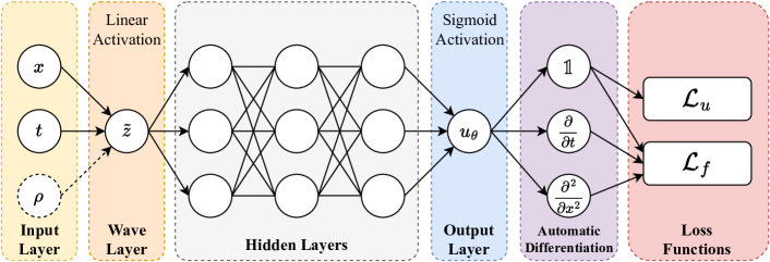
Figure 1: Schematic drawing of the wave-PINN that either approximates $u(x,t)$, or $u(x,t;\rho)$ by taking $\rho$ as an additional input variable. The additional wave layer (see Fig. 2) constrains the network function to $u_{\theta}(\tilde{z})$, thus ensuring the form of traveling wave solutions. The standard architecture does not use the wave layer. The generalizing architecture uses $\rho$ as an additional input.

3 Physics-Informed Neural Networks

A comprehensive description of PINNs can be found in [24]. For the sake of clarity, this section provides their fundamentals and discusses particular parts of the PINN framework needed in order to understand the modification being made in this work. In essence, PINNs represent a particular class of neural networks utilized for approximating solutions to differential equations by incorporating data- and physics-based soft constraints (or loss functions) during network training. The inputs to the network structure include the spatial and temporal coordinates of the physical system, though as it will be discussed shortly, they may not be limited to those variables. The network’s output corresponds to the targeted physical quantity; in this work, the concentration $u$ governed by Eq. (1). By selecting smooth activation functions for neurons in the hidden layers, e.g., hyperbolic tangent (tanh) or Sigmoid linear unit (swish), the network function is continuous over the (spatial-temporal) input domain. Accumulating all weights and biases of the network into a single network weight variable $\theta$, the network function is referred to as $u_{\theta}$.

3.1 Architectures

In this work, two distinct network architectures are tested: a standard architecture and a wave architecture. Additionally, the study comprises a network architecture designed for a discrete-$\rho$ approximation and a generalizing architecture for a continuous-$\rho$ approximation. The generalizing architecture considers the reaction rate coefficient as an additional input, thus approximates the solution for multiple values of $\rho$.

Standard and Wave Architectures. In the standard architecture, hidden layers directly follow the input layer, aiming to approximate the solution function in the general spatial-temporal form $u(x,t)$. Conversely, in the wave architecture, an additional wave layer is introduced directly after the input layer and before the hidden layers, see Fig. 1. The wave layer introduces a latent variable representation, as depicted in Fig. 2. The layer’s output is $\tilde{z}=\theta_{1}x+\theta_{2}t+\theta_{3}$, where $\theta_{1},\theta_{2}$, and $\theta_{3}$ represent trainable parameters. Consequently, the network function is compelled to adopt the traveling wave form $u(\tilde{z})$ as described in Eq. (5). It is essential to note that the additional bias term $\theta_{3}$ plays a crucial role, as data preprocessing steps, such as feature scaling, can significantly influence the effectiveness of a simpler representation with fewer parameters.

Generalization. This work also evaluates the capability of a single PINN instance in approximating solutions to Eq. (4) for multiple and continuous values of $\rho$. Referred to as the generalizing architecture, this is achieved by treating the reaction rate coefficient $\rho$ as an additional input parameter. The network architecture thus represents an approximation to a family of solutions in the form $u(x,t;\rho)$.

This additional input is either directly connected with the hidden layers (standard architecture) or processed in the wave layer (wave architecture). In the wave layer, the reaction rate coefficient is coupled with the spatio-temporal input variables through $\tilde{z}=\theta_{1}\rho_{1}x+\theta_{2}\rho_{2}t+\theta_{3}$, as captured by Fig. 2. Here, $\rho_{1}$ and $\rho_{2}$ are obtained through specific transformation used in the feature scaling which will be further discussed in Section 4.

Treating $\rho$ as an additional input variable enables a straightforward extension of the application of sampling schemes for collocation points.

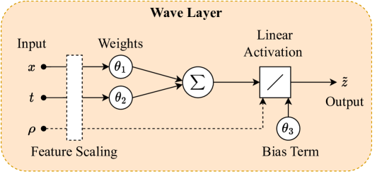
Figure 2: Schematic structure of the wave layer, which compresses the input variables into the form $\tilde{z}(x,t)=\theta_{1}x+\theta_{2}t+\theta_{3}$ for the single-$\rho$ approximation, or $\tilde{z}(x,t;\rho)=\theta_{1}\rho_{1}x+\theta_{2}\rho_{2}t+\theta_{3}$ when using the generalizing architecture.

3.2 Loss Functions

The data loss function encoding initial conditions (IC) and boundary conditions (BC) is given by

$$\mathcal{L}_{u}(\theta)=\frac{1}{N}\sum_{i=1}^{N}|u^{(i)}-u^{(i)}_{\theta}|^{2},$$ (8)

where $u^{(i)}_{\theta}$ denotes the network’s output to $N$ labeled data points.

The physics loss function evaluated on $N_{\mathrm{col}}$ collocation points, reads

$$\mathcal{L}_{f}(\theta)=\frac{1}{N_{\mathrm{col}}}\sum_{i=1}^{N_{\mathrm{col}}}\left|f^{(i)}_{\theta}\right|^{2},$$ (9)

and uses the physics residuals $f_{\theta}$ encoding Eq. (4) with

$$f_{\theta}(x,t;\rho)=\frac{\partial u_{\theta}}{\partial t}-\frac{\partial^{2}u_{\theta}}{\partial x^{2}}-\rho u_{\theta}(1-u_{\theta}).$$ (10)

Here, the dependency on the reaction rate coefficient $\rho$ is explicitly included to account for the formulation used by the generalizing architecture, while the dependency $u_{\theta}(x,t;\rho)$ is omitted for brevity. Both loss function are finally combined by the total loss function that reads

$$\mathcal{L}(\theta)=\mathcal{L}_{u}(\theta)+\mathcal{L}_{f}(\theta).$$ (11)

3.3 Residuals Weighting

It is well known that the standard PINN framework has issues with sharp and discontinuous solutions, which is discussed in [34], [35], [36], and [37]. As reported in [35], this phenomenon can be attributed to a paradoxical state at transition points, where the steep trend of the solution leads to nearly explosive behavior in the network derivatives and physics residuals in Eq. (10). Minimizing these residuals consequently results in reducing the network derivatives toward a smooth, potentially incorrect, solution that fails to capture the sharpness and steepness of the traveling wave. This will be verified through experiments in Section 5.1.

Reaction Term Weighting. Weighting the residuals has been already proposed as a remedy to cope with challenging solution functions [35, 36]. As a novel way of weighting the residuals for Fisher’s equation, and reaction-diffusion systems in general, a weighting scheme according to the strength of the reaction term $F$ is proposed. The motivation behind this lies in the fact that the sharpness of traveling waves is largely influenced by the reaction dynamics. In view of that, weighting each physics residual is performed according to

$$\omega=\frac{1}{\lambda|F(u_{\theta};\rho)|+1}.$$ (12)

Here, $\lambda$ is a hyperparameter that can be used to adjust the strength of the weighting, and trimmed to the particular problem given at hand. By weighting residuals according to Eq. (12), residuals in smooth regions with predominant diffusion consequently get a weight of $\omega\to 1$. However, weights of residuals in sharp regions are lowered, i.e. $\omega\to 0$, which effectively suppresses the effect of large gradients and physics loss residuals.

Using this weighting scheme in the definition of the physics loss function yields

$$\mathcal{L}_{f}(\theta)=\frac{1}{N_{\mathrm{col}}}\sum_{i=1}^{N_{\mathrm{col}}}\left|\omega^{(i)}f^{(i)}_{\theta}\right|^{2},$$ (13)

where a value of $\lambda=0$ corresponds to the unweighted form of the physics loss function as used by the conventional PINN framework.

Table 1: The four models employed in the study. These can be distinguished based on whether the physics loss function and/or the wave layer architecture are applied.

Model	Physics Loss	Wave Layer
standard-ANN
wave-ANN		✓
standard-PINN	✓
wave-PINN	✓	✓

4 Experimental Setup

For the experiments in the next section, four distinct models are employed that are listed in Table 1.

Data-driven ANNs. The first two models are data-driven ANNs which learn the solution function from labeled data, directly sampled from the analytical solution (7) and fed through the data loss function (8). The data is sampled anew at each training iteration, allowing access to an infinite number of training data points which is used to prevent overfitting. Notably, these models do not consider the physics loss function and hence serve as a reference for assessing how accurately the solution function can be learned purely from data. This setting is tested using both the standard architecture and the wave architecture, resulting in the two considered data-driven models.

PINNs. The two other models are PINN instances which apply the methodology discussed in Section 3. These models infer the solution functions by minimizing the loss function given by Eq. (11), where the data loss function is used to impose the IC and BC. This setting is also studied using both the standard architecture and the wave architecture.

Additionally, different settings for the residual weighting scheme are assessed, by considering $\lambda\in\{0,0.1,1,10\}$ as defined in Eq. (12). Notably, a value of $\lambda=0$ corresponds to the unweighted optimization, aligning with conventional PINNs optimization.

Computational Domain. To fully capture the traveling wave front for any $\rho$ within the computational domain, the domain is set with $x\in[-5,5]$ as the spatial domain and $t\in[0,0.004]$ as the temporal domain [38, 39, 41]. A diffusion coefficient with $\mu=10$ is considered and studied reaction rate coefficients are in the range $\rho\in[100,10.000]$.

Feature Scaling. Scaling the features in this study has proven to be essential for training any of the models within the chosen computational domain. Two distinct feature scaling strategies are employed, contingent on whether the standard or wave architecture is utilized. In the standard architecture, all input variables undergo scaling to the unit range $[0,1]$. Conversely, in the wave architecture, a different scaling strategy is implemented to ensure reduced sensitivity of the $\theta_{j}$ weights in the wave layer (refer to Fig. 2). This is achieved by leaving the spatial variable $x$ unscaled, while the temporal variable is scaled to the unit range $[0,1]$. The reaction rate input, however, undergoes a specific transformation given by $\rho_{1}\leftarrow\sqrt{\rho}$, while $\rho_{2}=\rho$, which is motivated by a commonly performed nondimensionalization step.

Data Settings. Due to the finite computational domain, IC and BCs are imposed by randomly sampling data from the analytical solution at the boundary of the computational domain. These data points are provided to the PINN through the data loss function. The collocation points are randomly sampled inside the computational domain using the Latin hypercube sampling scheme. Datasets for both IC/BCs and collocation data points are sampled anew at each training epoch with a default dataset size of $N=1024$, respectively. The data for the data-driven ANNs is also sampled anew at each epoch with a size of $N=1024$, to ensure that these models are trained at the same pace as the PINN models.

Network Settings. For the network architecture applied for discrete values of $\rho$, two hidden layers and 20 neurons per hidden layers are taken. The generalizing architecture, however, is applied with three hidden layers, and the same amount of neurons, to accommodate the increased complexity introduced by the additional dimension. The hyperbolic tangent (tanh) is used as hidden layer activation and the Sigmoid activation as output layer activation, to ensure that any prediction lies in the bounded interval $u_{\theta}\in[0,1]$. Various network sizes and activation functions have been evaluated, but qualitative conclusions remained consistent, hence results are presented for the aforementioned settings.

In all experiments, the Glorot weight initialization scheme is applied and Adam as the gradient-based optimization algorithm for minimizing the loss function given by Eq. (11). Optimization is carried out for $50k$ training epochs in the discrete-$\rho$ approximation and for $100k$ epochs in the continuous-$\rho$ approximation. A default learning rate of $0.001$ is used.

Performance Measure. The PINN’s performance is measure by means of the $L_{2}$-error which is defined as

$$L_{2}=\left(\frac{1}{N}\sum_{i=1}^{N}\left|u^{(i)}-u_{\theta}^{(i)}\right|^{2}\right)^{1/2},$$ (14)

where this is evaluated on randomly sampled data points from inside the computational domain with a dataset size of $N=10.000$.

5 Results

5.1 Discrete-$\rho$ Approximation

For the discrete-$\rho$ experiment, the model performance is evaluated by approximating the solution function for three individual reaction rate coefficients $\rho\in\{100,1.000,10.000\}$, training a separate model for each coefficient. Notably, with an increasing $\rho$ the solution function shifts to a sharp traveling wave since the computational domain is kept equal for all cases. Ten differently initialized instances are trained for each of the four models and each of the three coefficients.

Table 2: The mean (and standard deviations) of the $L_{2}$-error for the four tested models and different values for $\rho$. All numbers should be multiplied by $10^{-4}$. Bold: Best results.

		Reaction rate coefficient, $\rho$
Model	$\lambda$	100	1.000	10.000
standard-ANN	-	1.66 (1.30)	0.79 (0.29)	1.69 (2.10)
wave-ANN	-	1.12 (0.60)	1.05 (0.81)	1.54 (1.62)
standard-PINN	0	180 (46)	320 (184)	5689 (3469)
	0.1	37.9 (11.0)	81.1 (15.9)	36.8 (34.3)
	1	5.74 (0.95)	14.0 (3.0)	132 (66)
	10	1.72 (1.23)	8.79 (1.46)	354 (174)
wave-PINN	0	16.5 (13.5)	178 (160)	5082 (4106)
	0.1	1.26 (1.49)	1.65 (0.95)	12.1 (6.5)
	1	0.82 (0.95)	0.60 (0.63)	1.10 (0.80)
	10	2.16 (3.28)	0.83 (1.45)	3.11 (3.71)

Result Table. The results to this experiment can be found in Table 2, which displays the mean (and standard deviations) of the $L_{2}$-error for each tested model and setting. For the sake of clarity, the best result has been highlighted for each value of the reaction rate coefficient $\rho$.

Best Model. First, focus lies on the highlighted numbers in the table, which indicate, for each $\rho$, the model achieving the lowest $L_{2}$-error. Surprisingly, the wave-PINN with $\lambda=1$ achieves the lowest error for each tested reaction rate, even outperforming both data-driven ANNs. This result is particularly intriguing, as the data-driven ANNs have effectively (and without overfitting) learned the solution from the data, making them highly accurate for the given network size.

Standard vs. Wave. By comparing models using the standard and wave architecture, it can be generally found that the wave architecture performs better, with a substantial difference within the PINN models. The results clearly show that for nearly any PINN setting ($\lambda$), the wave architecture achieves lower prediction errors than the standard architecture. For the data-driven ANNs, the difference is less distinctive, with the standard architecture achieving slightly better results for a value of $\rho=1.000$.

Additionally, prediction plots for a single standard-PINN and wave-PINN instance, using $\lambda=1$, are presented in Fig. 3 and Fig. 4, respectively. It is evident from these figures that while both models visually align well with the reference solution, the wave-PINN consistently attains significantly lower prediction errors across the entire computational domain. Specifically, for the standard-PINN, errors are more pronounced at later time steps, suggesting issues in accurately capturing the speed at which the wave propagates. On the contrary, the largest errors in the wave-PINN are located along the traveling wave front, suggesting that it has effectively learned the correct wave speed. Notably, these errors remain orders of magnitude lower than those observed for the standard-PINN.

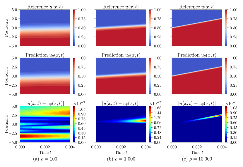
Figure 3: standard-PINN performance on Fisher’s equation using $\lambda=1$.

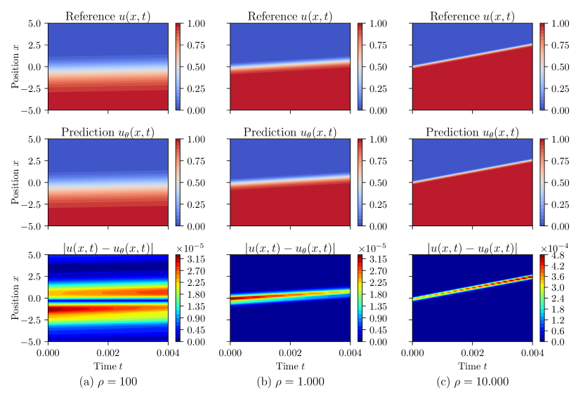
Figure 4: wave-PINN performance on Fisher’s equation using $\lambda=1$.

Optimal Residual Weighting. A discernible trend regarding the effectiveness of the proposed residual weighting scheme can be observed. The conventional, unweighted PINN optimization with $\lambda=0$ exhibits significant performance issues, particularly for large $\rho$ values as apparent from Table 2. The results further reveal that any form of residual weighting with $\lambda>0$ tends to mitigate these optimization challenges. Notably, a default choice of $\lambda=1$ consistently yields optimal results for the wave-PINN. However, for the standard-PINN, the optimal choice is less clear. For $\rho=100$ and $\rho=1,000$, $\lambda=10$ performs better, while for $\rho=10,000$, the weighting with $\lambda=0.1$ yields the best results.

Effectiveness of Residual Weighting. To further investigate the effectiveness of the residual weighting, the wave front for $\rho=10.000$ is illustrated in Fig. 5. In the figure, the left plot presents the true and predicted wave front for the time steps $t\in\{0.001,0.0015,0.002,0.0025,0.003\}$. The prediction is based on the fully trained wave-PINN that utilizes $\lambda=1$. Evaluated for this predicted solution, the weighted physics residuals along the wave front are shown in the right plot.

In particular, a weighting strength of $\lambda\in\{0,0.1,1,10\}$ is chosen to study the effects of the residuals weighting scheme in the right plot of Fig. 5. Apparent from the figure is that for the unweighted case ($\lambda=0$), physics residuals along the steep wave front take values orders of magnitude larger than residuals outside the wave front and in the smooth region. This coincides with findings discussed in [35], where it is expected that further optimization using $\lambda=0$ will drive away the accurately learned solution to a smoother, potentially incorrect wave front. It can be further observed that applying the residual weighting scheme with values $\lambda>0$ effectively reduces the strength of residuals along the wave front, which, in particular for $\lambda=1$, results in a more balanced allocation of physics residuals along the wave front. Notably, $\lambda=10$ further reduces the strength of the residuals along the wave front, which can take even smaller values than residuals in the smooth regions. This over-adjustment could explain why in Table 2 it is found that the wave-PINN with $\lambda=1$ achieves better results than with $\lambda=10$.

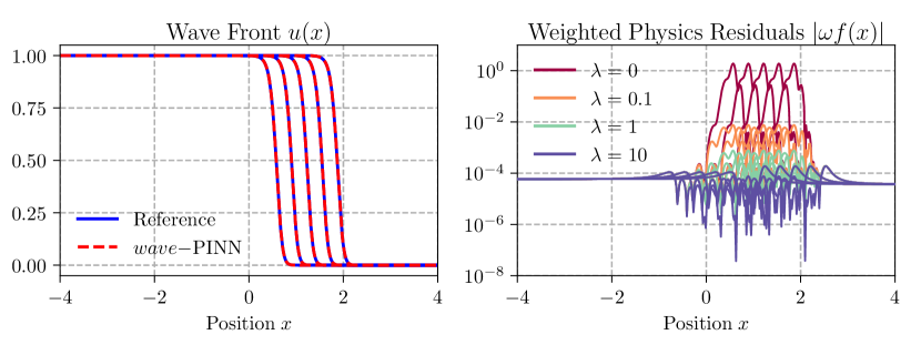
Figure 5: Wave front for $\rho=10.000$ and $t\in\{0.001,0.0015,0.002,0.0025,0.003\}$. Left: Reference solution and final prediction of the wave-PINN using $\lambda=1$. Right. Weighted physics residuals for different values of $\lambda$, assessed for the predicted solution function in the left plot. In the case of the unweighted scheme ($\lambda=0$), physics residuals at transition points on the wave front exhibit orders of magnitude larger values compared to those outside the wave front.

5.2 Continuous-$\rho$ Approximation

In this section, the generalizing network architecture is tested by incorporating $\rho$ as an additional input. Subsequently, the models approximate the solution $u(x,t;\rho)$ to Eq. (4) across the continuous parameterization domain $\rho\in[\rho_{\mathrm{min}},\rho_{\mathrm{max}}]$.

Assessing Interpolation Capability. A specific training strategy is applied to assess the data-driven ANN and PINN interpolation capability. In this approach, each model is trained using labeled data sampled from the analytical solution for two specific reaction rate coefficients, denoted as $\rho_{\mathrm{min}}$ and $\rho_{\mathrm{max}}$. Consequently, the interpolation task is to find good approximations within the continuous range $\rho\in[\rho_{\mathrm{min}},\rho_{\mathrm{max}}]$.

These coefficients define the boundaries of the computational domain in the $\rho$-dimension, and determine the range in which collocation points are uniformly sampled for the PINN models using Latin hypercube sampling. For the experiment, three distinct test cases are considered using different $\rho$-domains with $\rho_{\mathrm{min}}\in\{100,1.000\}$ and $\rho_{\mathrm{max}}\in\{1.000,10.000\}$. Again, ten differently initialized instances are trained for each model and setting.

Result Table. The results to this experiment can be found in Table 3, which displays the mean (and standard deviations) of the $L_{2}$-error for each tested model and setting. Notably, the $L_{2}$-error was assessed on a test set comprising $10.000$ data points, uniformly sampled across the domain $\rho\in(\rho_{\mathrm{min}},\rho_{\mathrm{max}})$. For the sake of clarity, the best result for each specific setting within the $\rho$-domain has been highlighted.

Best Model. Consistent with the results from the previous experiment, the wave-PINN achieves the lowest prediction error in all three cases. Interestingly, the wave-ANN also performs astonishingly well, with its errors marginally worse. This model, trained only on the two reaction rate coefficients $\rho_{\mathrm{min}}$ and $\rho_{\mathrm{max}}$, proves capable of achieving accurate interpolation within this range. Evidently, the incorporation of the wave layer provides a highly effective constraint that aids in finding solutions over a continuous parameterization.

Interpolation Performance. Having access to the solution function in the continuous form $u_{\theta}(x,t;\rho)$ allows to determine the $L_{2}$-error on the continuous $\rho$-domain where the modes were trained. This consideration is depicted in Figure 6, which illustrates the error curve for the model trained in the domain $\rho\in[100,10.000]$. Additionally, the two-dimensional wave front $u(x;\rho)$ for the last time step $t=0.004$ is plotted and shown in Figure 7.

Both figures demonstrate the outstanding performance of the wave-ANN and wave-PINN, with the latter clearly performing better in terms of the $L_{2}$-error (cf. Figure 6). This is also reflected in Figure 7 where the wave-PINN yields lower absolute errors along the continuous wave front $u(x;\rho)$.

Extrapolation Performance. Both wave models have indeed effectively learned the intrinsic structure of the parameterized solution function, as defined by Eq. (7). This is evident in Figure 6, where both models exhibit excellent performance throughout the plotted $\rho$-domain, extending beyond the confines of the training domain. Remarkably, even within the range of $\rho=100.000$, both models continue to provide strong approximations in the extrapolation regime, with only a slight degradation compared to the interpolation regime.

Comparing the two standard models, it is evident that the PINN performs better than the data-driven ANN, though their performance is not competitive with the wave models.

Table 3: The mean (and standard deviations) of the $L_{2}$-error for the four tested models over a specific domain $\rho\in(\rho_{\mathrm{min}},\rho_{\mathrm{max}})$. All numbers should be multiplied by $10^{-4}$. Bold: Best results.

$\rho_{\mathrm{min}}$		$\rho_{\mathrm{max}}$	standard-ANN	wave-ANN	standard-PINN	wave-PINN
100	-	1.000	110 (51)	1.83 (1.54)	5.16 (0.66)	1.46 (1.79)
1.000	-	10.000	559 (101)	3.21 (2.96)	173 (23)	1.83 (1.27)
100	-	10.000	1354 (120)	2.15 (2.23)	363 (45)	1.30 (1.69)

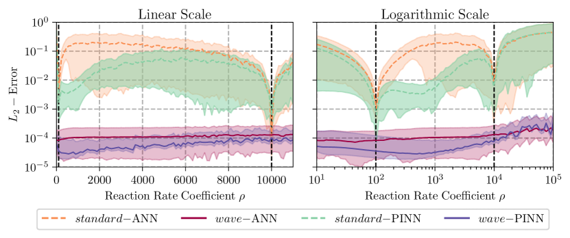
Figure 6: The median (and 25%- and 75%-quantiles) of the $L_{2}$-error for each tested model on the continuous domain $\rho\in[100,10.000]$. Labeled training data was used at $\rho=100$ and $\rho=10.000$, indicated by the dashed black lines.

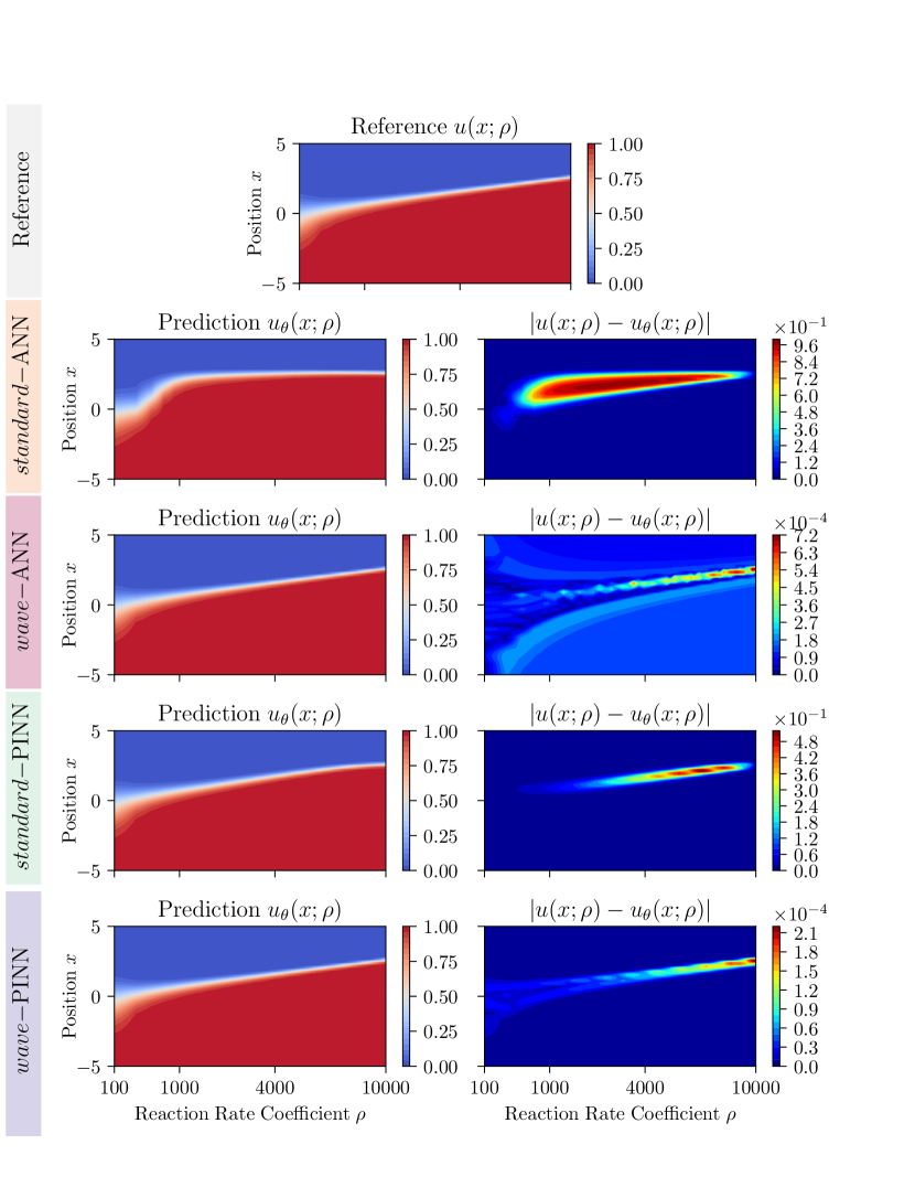
Figure 7: Prediction of the wave front $u(x)$ by a single model in the continuous $\rho$-space for the final time step $t=0.004$. For visualization purposes, the x-scale has been transformed using $\rho\leftarrow\sqrt{\rho}$.

6 Discussion & Future Work

The obtained results suggest that residual weighting schemes can overcome issues associated with sharp solutions as it is the case with steep propagating wave fronts in Fisher’s equation. The results presented in Table 2 and shown in Figure 5 resonate with the general discussion of standard PINNs struggling with approximating sharp solutions. Further modifications to the standard PINN framework are thus needed in order to overcome these difficulties.

The introduced residual weighting scheme is determined by the reaction term $F$, and reduces the weight of residuals in sharp regions with predominant reaction dynamics as evident from Figure 5. The basic idea of this approach is similar to what is proposed in [35]. However, in [35] the weighting scheme relies on the compressible property of hyperbolic PDEs which, consequently, is not directly applicable to reaction-diffusion systems as they are parabolic. Future work shall be dedicated to investigating the effectiveness of the proposed residual weighting scheme on more complex and general reaction mechanisms, e.g. of the form $\rho u(1-u^{q})$ with $q>0$, as introduced in [2].

The second investigation made in this work involved testing the wave architecture, specifically designed to approximate wave-like solutions in the form of $u(\tilde{z})$. As evident from the obtained results, the additional introduction of the wave layer proved highly effective in approximating solutions that take this particular form. The most remarkable difference between the standard and wave architecture is apparent in Table 3 and Figure 6.

One particularly interesting observation has been made in Table 2, where the wave-PINN exhibited superior performance compared to data-driven models explicitly trained on the analytical solution. Originally, the aim was to establish a performance benchmark for this network size to evaluate how closely the performance of PINNs would align with it. Surprisingly, the wave-PINN surpassed the data-driven models. Future investigations will aim to determine whether PINNs indeed provide a learning framework capable of surpassing purely data-driven models for specific learning tasks.

Finally, the generalizing architecture has been tested, which, in contrast to the discrete-$\rho$ approximation, provides an approximation to an entire family of solutions to Fisher’s equation in the form of $u(x,t;\rho)$. Extending the standard spatio-temporal input domain by an additional third dimension corresponding to the reaction rate coefficient $\rho$ offers a simple and effective approach to obtain multiple solutions at once by training only a single PINN instance.

Several questions still arise in this regard. For instance, what is the best approach to account for a particular parameterization? In the followed approach, the reaction rate coefficient $\rho$ appeared linearly in the governing differential equation, as shown in Eq. (4). Furthermore, the wave architecture was used with a specific feature scaling (see Section 4) that seemed highly suitable for the given problem. Specifically, by using $\rho_{1}\leftarrow\sqrt{\rho}$ and $\rho_{2}\leftarrow\rho$, a particular dependency was encoded into the model which was essential to train any of the wave models, thereby reducing the sensitivity of the weights $\theta_{j}$ in the wave layer. Importantly, this step was motivated by the commonly performed nondimensionalization step taking $\hat{x}\leftarrow\sqrt{\rho}x$ and $\hat{t}\leftarrow\rho t$.

Furthermore, having established a specific network architecture to account for the additional dimension, it would be interesting to know the best and most efficient approach to sampling the collocation points. Again, the linear dependence in the differential equations and the specific feature scaling seemed to align well with standard Latin hypercube sampling, which could explain the outstanding performance of the wave-PINN.

Future work should focus on extending the insights gained from this study. In particular, it would be interesting to further expand the discussed approach to address more complex reaction-diffusion systems and explore alternative PINN methods for solving differential equations across continuous parameterizations.

7 Conclusion

The rapid development of PINNs has endowed them with the capability to approximate solutions to differential equations. While the continuous parameterization of PINNs and their physics loss function offer significant flexibility in addressing various types of differential equations, it may also pose optimization challenges, especially in the presence of sharp solution functions. In this paper, PINNs were applied to solve Fisher’s equation with large reaction rate coefficients and sharp solutions representing steep traveling wave fronts. To address the challenges posed by sharp transitions in traveling waves, a residual weighting scheme was introduced and integrated into the optimization process of PINNs. The residual weighting scheme is based on the underlying reaction term and effectively facilitates optimization in sharp regions of the solution function. Additionally, a specific network architecture designed to approximate traveling waves was tested, and the results demonstrated outstanding improvements compared to conventional network architectures. Finally, a PINN architecture was explored that incorporates the reaction rate coefficient as an additional input, enabling the approximation of an entire family of solutions to Fisher’s equation. The results showcased that the PINN with the introduced modifications can effectively solve Fisher’s equation with large reaction rate coefficients and, furthermore, can be extended to approximate a family of sharp solutions with a single PINN instance.

References

- [1] Ronald Aylmer Fisher. The wave of advance of advantageous genes. Annals of eugenics, 7(4):355–369, 1937.
- [2] A Kolmogorov, I Petrovskii, and N Piskunov. Study of a diffusion equation that is related to the growth of a quality of matter, and its application to a biological problem. Moscow University Mathematics Bulletin, 1(1-26), 1937.
- [3] Mark J Ablowitz and Anthony Zeppetella. Explicit solutions of fisher’s equation for a special wave speed. Bulletin of Mathematical Biology, 41(6):835–840, 1979.
- [4] XY Wang. Exact and explicit solitary wave solutions for the generalised fisher equation. Physics letters A, 131(4-5):277–279, 1988.
- [5] Huaitang Chen and Hongqing Zhang. New multiple soliton solutions to the general burgers–fisher equation and the kuramoto–sivashinsky equation. Chaos, Solitons & Fractals, 19(1):71–76, 2004.
- [6] Nikolai A Kudryashov. Exact solitary waves of the fisher equation. Physics Letters A, 342(1-2):99–106, 2005.
- [7] Shan Zhao and Guo-Wei Wei. Comparison of the discrete singular convolution and three other numerical schemes for solving fisher’s equation. SIAM Journal on Scientific Computing, 25(1):127–147, 2003.
- [8] Kamel Al-Khaled. Numerical study of fisher’s reaction–diffusion equation by the sinc collocation method. Journal of Computational and Applied Mathematics, 137(2):245–255, 2001.
- [9] Jenö Gazdag and José Canosa. Numerical solution of fisher’s equation. Journal of Applied Probability, 11(3):445–457, 1974.
- [10] RC Mittal and Sumit Kumar. Numerical study of fisher’s equation by wavelet galerkin method. International Journal of Computer Mathematics, 83(3):287–298, 2006.
- [11] S Tang and RO11144430728 Weber. Numerical study of fisher’s equation by a petrov-galerkin finite element method. The ANZIAM Journal, 33(1):27–38, 1991.
- [12] Ramesh Chand Mittal and Rakesh Kumar Jain. Numerical solutions of nonlinear fisher’s reaction–diffusion equation with modified cubic b-spline collocation method. Mathematical Sciences, 7(1):12, 2013.
- [13] HS Shukla and Mohammad Tamsir. Extended modified cubic b-spline algorithm for nonlinear fisher’s reaction-diffusion equation. Alexandria Engineering Journal, 55(3):2871–2879, 2016.
- [14] Neeraj Dhiman and Mohammad Tamsir. A collocation technique based on modified form of trigonometric cubic b-spline basis functions for fisher’s reaction-diffusion equation. Multidiscipline Modeling in Materials and Structures, 14(5):923–939, 2018.
- [15] Mohammad Tamsir, Neeraj Dhiman, and Vineet K Srivastava. Cubic trigonometric b-spline differential quadrature method for numerical treatment of fisher’s reaction-diffusion equations. Alexandria engineering journal, 57(3):2019–2026, 2018.
- [16] Ali Şahin, İdris Dağ, and Bülent Saka. Ab-spline algorithm for the numerical solution of fisher’s equation. Kybernetes, 37(2):326–342, 2008.
- [17] Ali Başhan. Quartic b-spline differential quadrature method for solving the extended fisher-kolmogorov equation. Erzincan University Journal of Science and Technology, 12(1):56–62, 2019.
- [18] Ali Sahin and Ozlem Ozmen. Usage of higher order b-splines in numerical solution of fisher’s equation. International Journal of Nonlinear Science, 17(3):241–253, 2014.
- [19] RC Mittal and Sumita Dahiya. A study of quintic b-spline based differential quadrature method for a class of semi-linear fisher-kolmogorov equations. Alexandria Engineering Journal, 55(3):2893–2899, 2016.
- [20] Neeraj Dhiman, Amit Chauhan, Mohammad Tamsir, and Anand Chauhan. Numerical simulation of fisher’s type equation via a collocation technique based on re-defined quintic b-splines. Multidiscipline Modeling in Materials and Structures, 16(5):1117–1130, 2020.
- [21] Idiris Dag and Ozlem Ersoy. The exponential cubic b-spline algorithm for fisher equation. Chaos, Solitons & Fractals, 86:101–106, 2016.
- [22] Melis Zorsahin Gorgulu and Idris Dag. Exponential b-splines galerkin method for the numerical solution of the fisher’s equation. Iranian Journal of Science and Technology, Transactions A: Science, 42:2189–2198, 2018.
- [23] Mohammad Tamsir, Vineet K Srivastava, Neeraj Dhiman, and Anand Chauhan. Numerical computation of nonlinear fisher’s reaction–diffusion equation with exponential modified cubic b-spline differential quadrature method. International Journal of Applied and Computational Mathematics, 4:1–13, 2018.
- [24] Maziar Raissi, Paris Perdikaris, and George E Karniadakis. Physics-informed neural networks: A deep learning framework for solving forward and inverse problems involving nonlinear partial differential equations. Journal of Computational physics, 378:686–707, 2019.
- [25] Xiaowei Jin, Shengze Cai, Hui Li, and George Em Karniadakis. Nsfnets (navier-stokes flow nets): Physics-informed neural networks for the incompressible navier-stokes equations. Journal of Computational Physics, 426:109951, 2021.
- [26] Hamidreza Eivazi, Mojtaba Tahani, Philipp Schlatter, and Ricardo Vinuesa. Physics-informed neural networks for solving reynolds-averaged navier–stokes equations. Physics of Fluids, 34(7), 2022.
- [27] Wafaa Mohamed Shaban, Khalid Elbaz, Annan Zhou, and Shui-Long Shen. Physics-informed deep neural network for modeling the chloride diffusion in concrete. Engineering Applications of Artificial Intelligence, 125:106691, 2023.
- [28] Shengze Cai, Zhicheng Wang, Sifan Wang, Paris Perdikaris, and George Em Karniadakis. Physics-informed neural networks for heat transfer problems. Journal of Heat Transfer, 143(6):060801, 2021.
- [29] Weiqi Ji, Weilun Qiu, Zhiyu Shi, Shaowu Pan, and Sili Deng. Stiff-pinn: Physics-informed neural network for stiff chemical kinetics. The Journal of Physical Chemistry A, 125(36):8098–8106, 2021.
- [30] Enrico Schiassi, Mario De Florio, Barry D Ganapol, Paolo Picca, and Roberto Furfaro. Physics-informed neural networks for the point kinetics equations for nuclear reactor dynamics. Annals of Nuclear Energy, 167:108833, 2022.
- [31] Jiangong Pan, Xufeng Xiao, Lei Guo, and Xinlong Feng. A high resolution physics-informed neural networks for high-dimensional convection–diffusion–reaction equations. Applied Soft Computing, 148:110872, 2023.
- [32] Katsiaryna Haitsiukevich and Alexander Ilin. Improved training of physics-informed neural networks with model ensembles. In 2023 International Joint Conference on Neural Networks (IJCNN), pages 1–8. IEEE, 2023.
- [33] Homayoon Tarbiyati and Behzad Nemati Saray. Weight initialization algorithm for physics-informed neural networks using finite differences. Engineering with Computers, pages 1–17, 2023.
- [34] Aditi Krishnapriyan, Amir Gholami, Shandian Zhe, Robert Kirby, and Michael W Mahoney. Characterizing possible failure modes in physics-informed neural networks. Advances in Neural Information Processing Systems, 34:26548–26560, 2021.
- [35] Li Liu, Shengping Liu, Hui Xie, Fansheng Xiong, Tengchao Yu, Mengjuan Xiao, Lufeng Liu, and Heng Yong. Discontinuity computing using physics-informed neural network. arXiv preprint arXiv:2206.03864, 2022.
- [36] Zhiping Mao and Xuhui Meng. Physics-informed neural networks with residual/gradient-based adaptive sampling methods for solving partial differential equations with sharp solutions. Applied Mathematics and Mechanics, 44(7):1069–1084, 2023.
- [37] Mario De Florio, Enrico Schiassi, Francesco Calabrò, and Roberto Furfaro. Physics-informed neural networks for 2nd order odes with sharp gradients. Journal of Computational and Applied Mathematics, 436:115396, 2024.
- [38] Daniel Olmos and Bernie D Shizgal. A pseudospectral method of solution of fisher’s equation. Journal of Computational and Applied Mathematics, 193(1):219–242, 2006.
- [39] Shengtai Li, Linda Petzold, and Yuhe Ren. Stability of moving mesh systems of partial differential equations. SIAM Journal on Scientific Computing, 20(2):719–738, 1998.
- [40] Yiqi Qiu and DM1654948 Sloan. Numerical solution of fisher’s equation using a moving mesh method. Journal of Computational Physics, 146(2):726–746, 1998.
- [41] RC Mittal and Geeta Arora. Efficient numerical solution of fisher’s equation by using b-spline method. International Journal of Computer Mathematics, 87(13):3039–3051, 2010.