Reinforcement Learning for Docking Maneuvers with Prescribed Performance

Abstract

We propose a two-component data-driven controller to safely perform docking maneuvers for satellites. Reinforcement Learning is used to deduce an optimal control policy based on measurement data. To safeguard the learning phase, an additional feedback law is implemented in the control unit, which guarantees the evolution of the system within predefined performance bounds. We define safe and safety-critical areas to train the feedback controller based on actual measurements. To avoid chattering, a dwell-time activation scheme is implemented. We provide numerical evidence for the performance of the proposed controller for a satellite docking maneuver with collision avoidance.

1 Introduction

In recent years, traffic in space has significantly increased with new players sending satellites to space and old spacecrafts tumbling around as space debris. This adds further complexity to safely perform docking maneuvers in space since collision may damage and destroy, e.g., satellites causing significant delays in operational tasks and high additional costs. Furthermore, the ground station can only intervene time delayed. This motivates us to develop an automatic controller, which ensures successful and collision-free completion of docking maneuvers in space.

In general, path planning and collision avoidance is done by solving optimal control problems. Therefore, one defines an objective function and constraints, which include the equations of motion of the dynamical system as well as collision constraints. Typically, dynamic programming approaches are well suited to solve collision-constrained optimal control problems. However, for docking maneuvers, the combination of high complexity, a large number of degrees of freedom, and variability w.r.t. initial conditions push classical optimal-control approaches to their limits. Recently, following the path of artificial intelligence, Reinforcement Learning (cf. Bertsekas (2019)) approaches have emerged as a remedy. These data-based control approaches can handle high degrees of freedom and various scenarios without recomputing optimal control solutions. Instead of solving slight variations of the optimal control problem over and over again, it is sufficient to just execute the trained policy, e.g., a neural network, acting as a fast online controller. However, so far, not much is known about performance guarantees for such control strategies, which is highly relevant for safety critical control tasks such as collision avoidance during docking maneuvers. Thus, as an additional safeguarding mechanism, we use the funnel controller proposed in Ilchmann et al. (2002). Funnel control is a high-gain adaptive feedback controller with the following two advantages: First, it achieves tracking of a given reference trajectory $y_{\rm ref}$ within predefined error margins. This means that the output $y$ satisfies $\|y(t)-y_{\rm ref}(t)\|<\psi(t)$ for all $t\geq 0$ for a prespecified error tolerance $\psi(t)>0$. Second, the tracking is achieved for unknown nonlinear multi-input multi-output systems. We highlight that no system equations are required; rather the following structural assumptions are made: well-defined relative degree, bounded-input bounded-output stable internal dynamics, and a high-gain property. The latter means that the system can react sufficiently fast if only the input is excited by a large enough signal – a key property for high-gain adaptive control with prescribed accuracy. Combining funnel control with other control strategies has been topic in recent research, e.g., in Berger et al. (2021a); Drücker et al. (2023) in combination with feedforward control, in Berger et al. (2023); Lanza et al. (2023a) robustifying model predictive control, and in Lanza et al. (2023b); Schmitz et al. (2023) in the context of sampled-data control of continuous-time nonlinear systems, to name but a few.

In Saxena et al. (2023), the authors present a Reinforcement Learning approach, in which the design of rewards for deep Q-learning builds upon funnel functions, for learning a control policy that enforces some Signal Temporal Logic specifications. In Xia et al. (2023), the authors present a robust Reinforcement Learning control strategy that includes motion constraints for a vertical take-off and landing of an unmanned aerial vehicle on a moving target. In Elhaki et al. (2023), the authors use actor-critic neural networks to come up with a controller that has a prescribed-performance funnel for surface vessel models. In Berthier (2022) and Berthier et al. (2021), a trajectory tracking problem is presented for a floating satellite with commanded torques. We emphasize that the floating satellite in this manuscript surpasses the satellites model in its complexity.

The main contribution of this publication is to add a robustness component to the training phase of a Reinforcement Learning based controller such that the obtained policy guarantees to stay within a prescribed safety region. Previous work has already addressed the construction of a tracking controller with prescribed performance for nonlinear systems including a safeguard component in the learning process, cf. Lanza et al. (2023b); Schmitz et al. (2023). Here, we build upon these results and enhance the Reinforcement Learning framework allowing for other control strategies than Q-learning as well. Moreover, we level its applicability to more complicated control systems such as the control of satellites in space, represented by a sophisticated satellite model.

This manuscript is structured as follows. In Section 2, we model the satellite, which is equipped with a robot arm for docking maneuvers. Furthermore, we investigate its mathematical properties and verify the assumptions required to apply funnel control. In Section 3, we introduce the overall control objective, the Reinforcement Learning policy, and the funnel controller. Then, we present our novel methodology combining RL and funnel control. To avoid continuous action of the funnel controller, we implement an activation function and use a dwell-time scheme to prevent chattering. In Section 4, we illustrate the two-component learning-based controller via a numerical simulation of a docking maneuver in orbit.

Notation. $\mathds{R}_{\geq 0}:=[0,\infty)$. For $k\leq m\leq n\in\mathds{N}$ and $v\in\mathds{R}^{n}$ we denote with $u_{k:m}$ the components $(v_{k},\ldots,v_{m})\in\mathds{R}^{m-k+1}$. $W^{k,\infty}(I,\mathds{R}^{n})$ is the Sobolev space of all $k$-times weakly-differentiable functions $f:I\to\mathds{R}^{n}$ with $f,\dots,f^{(k)}$ essentially bounded. $0_{n\times m}$ for $m,n\in\mathds{N}$ represents a zero matrix with $n$ rows and $m$ columns. Furthermore, with $\mathbb{1}_{n\times n}$ we denote an $n\times n$ identity matrix.

2 Modeling the satellite

In this section, we model the satellite as multibody system. We follow the steps from the book of Kortüm and Lugner (1993). The general structure of the satellite can be seen in Figure 1. It consists of a satellite body, which is described by the Cartesian coordinates of its center of mass $[x,y,z]$ as well as its roll $\phi$, pitch $\theta$ and yaw $\psi$ angle. Furthermore, attached to this body, we assume to have a robot arm. This arm consists of two elements. One is directly linked to the satellite’s body. The spherical joint allows two degrees of freedom ($\psi_{1}$,$\theta_{1}$). The second element of the robot arm is attached to the first one by a revolute joint ($\theta_{2}$). We assume that we can manipulate the satellite by applying

• forces to accelerate the satellite body in $x$-, $y$- and $z$-direction,

• angular momentum to the satellite body and

• angular momentum to the robot arm.

In total, we have nine independent control inputs. The parameters of the satellite can be found in Table 1.

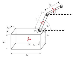
Figure 1: Schematic representation of the satellite model.

Table 1: Parameters of the Satellite Model

Variable	Unit	Value	Description
$m_{1}$	[kg]	$10$	mass of satellite body
$m_{2}$	[kg]	$1$	mass of first robotic link
$m_{3}$	[kg]	$1$	mass of second robotic link
$l_{s}$	[m]	$1$	length of satellite body
$b_{s}$	[m]	$0.5$	width of satellite body
$h_{s}$	[m]	$0.5$	height of satellite body
$r_{1}$	[m]	$0.1$	radius of first robotic link
$r_{2}$	[m]	$0.1$	radius of second robotic link
$l_{1}$	[m]	$1$	length of first robotic link
$l_{2}$	[m]	$1$	length of second robotic link
$p_{x}$	[m]	$0.4$	x-distance from center of gravity
			of satellite body to mount point
$p_{z}$	[m]	$0.25$	z-distance from center of gravity
			of satellite body to mount point

For the derivation of the equations of motion, we introduce $q_{1}=[x,y,z,\phi,\theta,\psi]^{\top}$ as well as $q_{2}=[\theta_{1},\psi_{1},\theta_{2}]^{\top}$. Following the steps from Kortüm and Lugner (1993), the equations of motion read

$$M(q_{1}(t),q_{2}(t))\ddot{q}_{1}(t) =f(t,\dot{q}_{1}(t),\dot{q}_{2}(t),q_{1}(t),q_{2}(t))$$

$$\quad+g(q_{1}(t),q_{2}(t))^{\top}u_{1:6}(t),$$

$$\ddot{q}_{2}(t) =u_{7:9}(t),$$

where $u(t)\in\mathds{R}^{9}$ represent the control inputs. Please note that from now on we will suppress the time dependencies of all quantities in this section for better readability. We define the output

$$y=\begin{bmatrix}q_{1}\\ q_{2}\end{bmatrix},$$

and may write the equations of motion in input/output form

$$\ddot{y} =\begin{bmatrix}M(y)^{-1}f(t,\dot{y},y)\\ 0_{3x1}\end{bmatrix}+\begin{bmatrix}M(y)^{-1}g(y)^{\top}&0_{3x3}\\ 0_{3x3}&\mathbb{1}_{3x3}\end{bmatrix}u.$$ (1)

To check the assumption in order to apply the funnel theory, we need to check the positive definiteness of the matrix

$$B(q_{1},q_{2}):=\text{diag}\left(M(q_{1},q_{2})^{-1}g(q_{1},q_{2})^{\top},\mathbb{1}_{3x3}\right).$$

Because of the block diagonal structure of this matrix, we can focus on the upper left block. Therefore, we focus on the mass matrix $M(q_{1},q_{2})$ and the matrix $g(q_{1},q_{2})$. Due to their long forms, we omit to write down the exact representation of the mass matrix $M$ and the matrix $g$. Instead, we introduce the center of mass $r_{i}(q_{1},q_{2})$ and the angular velocity $\omega_{i}(q_{1},q_{2})$ of body $i$. Together with the corresponding Jacobians

$$J_{i}=\frac{\partial r_{i}(q_{1},q_{2})}{\partial q_{1}},\quad\text{for }i=1,2,3,$$

$$J_{i\omega}=\frac{\partial\omega_{i}(q_{1},q_{2})}{\partial q_{1}},\quad\text{for }i=1,2,3,$$

and the moments of inertia $I_{i}$ of body $i$, the mass matrix can be represented as:

$$M(q_{1},q_{2})=\sum_{i=1}^{3}m_{i}J_{i}^{T}J_{i}+J_{i\omega}^{T}I_{i}J_{i\omega}.$$

Because of its structure, we can directly deduce that the mass matrix is symmetric and positive semi-definite. Moreover, for $\theta\neq-\frac{\pi}{2}$ it is positive definite. Since $M(q_{1},q_{2})$ is positive definite, we know that its inverse is positive definite as well. Similar, the matrix $g$ reads

$$g(q_{1},q_{2})^{\top} =\begin{bmatrix}J_{1}^{\top}A_{z}(\psi)A_{y}(\theta)A_{x}(\phi)\\ J_{1\omega}^{\top}\end{bmatrix}$$

with the rotation matrices:

$$A_{x}(\phi) =\begin{bmatrix}1&0&0\\ 0&\cos(\phi)&-\sin(\phi)\\ 0&-\sin(\phi)&\cos(\phi)\\ \end{bmatrix},$$

$$A_{y}(\theta) =\begin{bmatrix}\cos(\theta)&0&-\sin(\theta)\\ 0&1&0\\ -\sin(\theta)&0&\cos(\theta)\\ \end{bmatrix},$$

$$A_{z}(\psi) =\begin{bmatrix}\cos(\psi)&-\sin(\psi)&0\\ -\sin(\psi)&\cos(\psi)&0\\ 0&0&1\\ \end{bmatrix}.$$

The symbolic inversion of the mass matrix is computationally complex. Because of the bijection defined by $w=M^{-1}v$ for $v\in\mathds{R}^{6}$ and the transformation

$$v^{\top}M^{-1}g^{\top}v =v^{\top}M^{-1}g^{\top}M^{\top}M^{-\top}v$$

$$=(M^{-\top}v)^{\top}g^{\top}M^{\top}(M^{-\top}v)$$

$$=w^{\top}g^{\top}M^{\top}w$$

$$=w^{\top}g^{\top}Mw,$$

we focus on the positive definiteness of the matrix $g^{\top}M$. We verified numerically that the matrix $g^{\top}M+(g^{\top}M)^{\top}$ has only positive eigenvalues for $\phi,\theta,\psi\in[-\frac{\pi}{8},\frac{\pi}{8}]$ and $\theta_{1},\psi_{1},\theta_{2}\in[-\pi,\pi]$. Hence, system (1) has well-defined relative degree two in the set

$$\mathbb{X}:=\left\{\begin{bmatrix}q_{1}\\ q_{2}\end{bmatrix}\in\mathds{R}^{9}|\phi,\theta,\psi\in\left[-\frac{\pi}{8},\frac{\pi}{8}\right],\theta_{1},\psi_{1},\theta_{2}\in[-\pi,\pi]\right\}.$$

From this we directly deduce that the system has the high-gain property, cf. (Berger et al., 2021b, Rem. 1.3), and moreover, it has trivial (and thus stable) internal dynamics in $\mathbb{X}$. Therefore, system (1) is accessible for funnel control in the above indicated area. This means that, starting in $\mathbb{X}$, funnel control can be used to force the system to evolve within this area, cf. (2).

3 Control objective and controller

In this section, we introduce the control objective and the two-component controller to achieve that objective.

3.1 Control objective

The aim is to use Reinforcement Learning to derive an (optimal) control strategy from system data to perform a docking maneuver in space. To safeguard the learning phase, the data-driven controller is equipped with an additional feedback controller (funnel control). This feedback controller is capable to compensate possible undesired control actions such that the output $y=(q_{1},q_{2})$ of the system follows a given trajectory $y_{\rm ref}$ with prescribed accuracy, i.e.,

$$\forall\,t\geq 0\,:\ \|y(t)-y_{\rm ref}(t)\|<1/\varphi(t)$$ (2)

for a user defined error tolerance $\varphi$. This situation is illustrated in Figure 2(a). Requirements on the reference $y_{\rm ref}$ and the funnel boundary function $\varphi$ are presented in detail in Section 3.3.

(a) Evolution of the error $e$ within boundary $1/\varphi$.

(b) Safe (green) and safety-critical (red) region for $e_{2}$.

Figure 2: Tracking error and funnel boundary.

3.2 Reinforcement Learning

As we know from Section 2, the satellite motion is described by $18$ variables ($q_{1}$, $q_{2}$, $\dot{q}_{1}$ and $\dot{q}_{2}$). This high complexity pushes classical optimal control approaches to their limits. However, AI approaches have shown that they can cope with high-dimensional problems. Thus, we apply the Proximal Policy Optimization (PPO) algorithm from Schulman et al. (2017). In order to apply an RL approach, we need to define the underlying Markov Decision Process:

• State space $S$: states of the satellite $[q_{1}^{\top}\,q_{2}^{\top}\,\dot{q}_{1}^{\top}\,\dot{q}_{2}^{\top}]^{\top}$.

• Action space $A$: set of feasible control values, i.e., $[-0.15,0.15]^{9}$.

• The transition probability does not have to be specified explicitly. Trajectories are generated with the above introduced model.

• The initial position of the satellite is $s_{0}=0_{18\times 1}$.

• Reward function $r:S\times A\rightarrow\mathds{R}$ will be defined in Section 4.

The idea of model-free online RL is based on the interaction between policy and environment in the form of a feedback loop. Typically, this control loop is defined for a discrete-time framework. Thus, we introduce the equidistant discretization points $t_{0}<t_{1}<\dots<t_{N}$ with $N\in\mathds{N}$ and $\Delta h=t_{k+1}-t_{k}$ for all $k=1,\dots,N-1$. Thereon, the RL algorithm can be applied.

PPO is a gradient based RL approach, which iteratively improves a parametrized policy $\pi_{\mu}:A\times S\rightarrow\mathds{R}_{+}$ for parameters $\mu$. This randomized policy $\pi_{\mu}(\cdot,s)$ for $s\in S$ provides a density, from which the next action/control can be sampled. The usual target function in RL is

$$\max_{\mu}\mathds{E}_{\tau}\left[\sum_{k}\gamma^{k}r(s_{k},a_{k})\right],\quad 0<\gamma\leq 1,$$

where $\mathds{E}_{\tau}$ represents the expected value over all possible trajectories $\tau=[s_{0}^{\top},a_{0}^{\top},\dots,s_{N}^{\top}]^{\top}$ of length $N\in\mathds{N}$. In this manuscript, we make use of an extension of this expression by a trust region idea, where the Kullback-Leibler divergence measures the difference of policies. Thereby, the trust region is not handled as hard constraint, but as penalty term. We refer to Schulman et al. (2015, 2017) for details.

Finally, the actual control $a_{k}$ given by RL for the current state $s_{k}\in S$ is sampled from the parameterized policy. Hence, the RL feedback law $u_{\text{RL}}$ is given as

$$u_{\text{RL}}(t)=a_{k}\sim\pi_{\mu}(\cdot,s_{k})\qquad\text{for $t\in[t_{k},t_{k+1})$, $k\in\mathds{N}$.}$$ (3)

We stress that, usually, the policy and the Markov Decision Process are tailored to time-discrete control systems. In this manuscript, the RL control $u_{\text{RL}}$ is assumed to be a sampled-data control as it can be seen in (3). In this way, the discrete-time and continuous-time frameworks of RL and the funnel controller can be combined.

3.3 Safeguarding feedback law

In this section we present the second controller component, namely the so-called funnel controller. This is a high-gain adaptive controller, which achieves output reference tracking within prescribed error bounds (2). Since this controller is model-free, it safeguards the learning process by compensating undesired control effects from the RL component. For a given funnel function $\varphi:\mathds{R}_{\geq 0}\to\mathds{R}_{>0}$ belonging to the set

$$\Phi:=\left\{\ \varphi\in W^{1,\infty}(\mathds{R}_{\geq 0},\mathds{R})\ \left|\ \vphantom{\varphi\in W^{1,\infty}(\mathds{R}_{\geq 0},\mathds{R})}\inf_{s\geq 0}\varphi(s)>0\ \right.\right\},$$

and given reference $y_{\rm ref}\in W^{2,\infty}(\mathds{R}_{\geq 0},\mathds{R}^{m})$, we formally introduce the funnel control feedback. First, in virtue of Berger et al. (2021b) we introduce the following auxiliary variables

$$e(t) :=\begin{bmatrix}q_{1}(t)\\ q_{2}(t)\end{bmatrix}-\begin{bmatrix}q_{1,\text{ref}}(t)\\ q_{2,\text{ref}}(t)\end{bmatrix},$$ (4)

$$e_{1}(t) :=\varphi(t)e(t),$$

$$e_{2}(t) :=\varphi(t)\dot{e}(t)+\frac{1}{1-\lVert e_{1}(t)\rVert^{2}}e_{1}(t)$$

$$=\varphi(t)\left(\dot{e}(t)+\frac{1}{1-\lVert e_{1}(t)\rVert^{2}}e(t)\right).$$

with $e(t)=e(t,y)$, $e_{1}(t)=e_{1}(t,y)$, and $e_{2}(t)=e_{2}(t,y,\dot{y})$. The funnel control feedback law then reads

$$u_{\text{funnel}}(t)=-\frac{1}{1-\lVert e_{2}(t)\rVert^{2}}e_{2}(t).$$ (5)

This control law is of adaptive high-gain type. The intuition is the following. If the tracking error is small, then the distance to the error boundary $1/\varphi(t)$ is large and no/little input action is required to achieve the tracking task. If, however, the tracking error approaches its tolerance, then the denominator $1-\varphi(t)^{2}\|e(t)\|^{2}$ becomes small, and hence, the fraction becomes large. Thus, the error is “pushed away” from the funnel boundary and satisfies (2) for all times. We highlight that, although in (5) a possible pole is introduced, it has been proven that the control input is finite for all times, i.e., the error never touches the funnel boundary, cf. Ilchmann et al. (2002) for relative degree one, and Berger et al. (2021b) for arbitrary relative degree.

3.4 Combined controller

To achieve the control objective introduced in Section 3.1, we combine the two controller components. One first approach could be to set

$$u:=u_{\text{funnel}}+u_{\text{RL}}.$$

However, in this case the funnel controller (5) would be active whenever $e_{2}(t)\neq 0$ and thus, evaluation of the effectiveness of $u_{\rm RL}$ is not possible, since $u_{\rm FC}$ continuously intervenes – even if RL provides a potentially better control signal due to, e.g., its prediction capabilities. Therefore, we divide the interior of the funnel into a safe and a safety-critical region, cf. Figure 2(b). More precise, we introduce an activation threshold $\lambda\in[0,1)$ to divide the (half-open) interval $[0,1)$ into a safe and a safety-critical region and evaluate the auxiliary variable $e_{2}(t)$ w.r.t. the activation threshold, cf. Schmitz et al. (2023); Lanza et al. (2023b). For a given $\lambda\in(0,1)$ we define the activation function $\tilde{\alpha}:[0,1)\to[0,1)$ by

$$\tilde{\alpha}(s)=\max\{0,\|e_{2}(t)\|-\lambda\}$$

With this, we could define the overall controller

$$u:=\tilde{\alpha}(\|e_{2}(t)\|)\cdot u_{\text{funnel}}+u_{\text{RL}},$$

where the funnel controller is only active, if the auxiliary signal $e_{2}$ exceeds the activation threshold $\lambda$. However, this controller is likely to lead to chattering behavior, since whenever $e_{2}$ touches the activation threshold, the funnel controller would react and may achieve $\|e_{2}\|<\lambda$ immediately. To avoid possible chattering in the control signal, we introduce a dwell-time activation scheme for the funnel controller as follows

$$\alpha_{t_{d}}(t,e_{2}(t))=\max\left\{0,\max_{s\in[t-t_{d},t]}\|e_{2}(s)\|-\lambda\right\}$$

where $t_{d}>0$ is a preassigned dwell time. The previous function “records” if the auxiliary variable has exceeded or is above the activation threshold within the past interval of length $t_{d}$. With this activation function, we define the overall control law

$$u:=\alpha_{t_{d}}(t,e_{2}(t))\cdot u_{\text{funnel}}+u_{\text{RL}}.$$ (6)

Based on the previous considerations, we may formulate the following feasibility result for the two-component controller.

Theorem 1

Consider system (1). Let a reference trajectory $y_{\rm ref}\in W^{2,\infty}(\mathds{R}_{\geq 0},\mathds{R}^{9})$ and performance bound $\varphi\in\Phi$ be given. If the auxiliary variables (4) satisfy the initial conditions $\varphi(0)\|e_{1}(0)\|<1$ and $\varphi(0)\|e_{2}(0)\|<1$, then the proposed controller (6) achieves the control objective (2).

We argue that the funnel control theory can be applied in the current setting. First we observe that the control $u_{\rm RL}$ from (3) is piecewise constant and in particular bounded. Since the arguments to show boundedness of the closed-loop signals in funnel control apply in a small neighborhood inside the funnel boundary (cf. proof of (Berger et al., 2021b, Thm. 1.9)), the incorporation of the activation function does not jeopardize applicability of these arguments.

4 Numerical example

We illustrate the above introduced controller (6) in a docking maneuver scenario. The goal is to reach a predefined position with the arm of the satellite. Meanwhile, the satellite body should move as little as possible. This is a nontrivial task since a change in the arm’s position always leads to a force acting on the satellite body. Furthermore, we add collision areas where the rewards become negative. These areas represent solar panels, antennas or other objects, which might be part of the target satellite and which we do not want to touch to avoid damage.

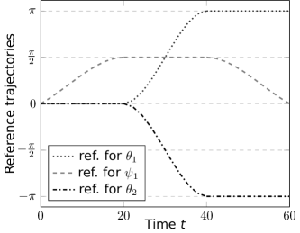
Figure 3: Reference trajectory for $\theta_{1}$, $\psi_{1}$ and $\theta_{2}$.

With respect to these constraints, we define a reference trajectory, which is safe:

$$y_{1,\text{ref}}(t) =0_{6\times 1},\forall t\in[0,60],$$

$$y_{2,\text{ref}}(t) =\begin{cases}\begin{bmatrix}0,&p_{1}\left(t\right),&0\end{bmatrix}^{\top},\text{if }t\leq 20,\\ \begin{bmatrix}p_{2}\left(t\right),&\frac{\pi}{2},&-p_{2}\left(t\right)\end{bmatrix}^{\top},\text{if }20<t\leq 40,\\ \begin{bmatrix}\pi,&p_{3}\left(t\right),&-\pi\end{bmatrix}^{\top},\text{if }40<t,\end{cases}$$

with $$p_{1}(t):=\frac{-\pi}{16000}t^{3}+\frac{\pi}{800}t^{2}+\frac{\pi}{40}t,$$

$$p_{2}(t):=\frac{-\pi}{4000}\left(t-20\right)^{3}+\frac{3\pi}{400}\left(t-20\right)^{2},$$

$$p_{3}(t):=\frac{\pi}{16000}\left(t-40\right)^{3}-\frac{\pi}{400}\left(t-40\right)^{2}+\frac{\pi}{2}.$$

The reference trajectory $y_{2,\text{ref}}(t)$ is depicted in Figure 3. We stress that it is not the goal to just follow the reference trajectory. Instead, the reference trajectory only reveals a collision free trajectory, in whose neighborhood the final trajectory is to be found. For this scenario, we assume the limiting funnel for the deviation from the reference trajectory:

$$\varphi(t)=8/\pi.$$

It is important to note that within the funnel the positive definiteness of the matrix $g^{\top}M$ is guaranteed. This means that we can apply the funnel control and it will guarantee that we will not leave the set $\mathbb{X}$. Inside this area, we can define the actual task for the PPO algorithm. This is done by introducing the reward functions. For a better comparability, we run the same RL algorithm without an additional funnel controller. Thus, we distinguish between the reward function for the algorithm, which is supported by a funnel controller, denoted by $r_{\text{funnel}}$ and for a classical pure RL algorithm, denoted by $r$. For $s_{k}\in S$ and $a_{k}\in A$ at time $t_{k}$, we define:

$$r_{\text{funnel}}\left(s_{k},a_{k}\right)\\ =\frac{(1-\lVert e\rVert)}{10}-\int_{t_{k}}^{t_{k+1}}\alpha_{t_{d}}(t,e_{2})\lVert u_{\text{funnel}}(t)-u_{\rm RL}(t)\rVert\,\text{d}t.$$

We point out that the second part of the reward function forces the RL policy to avoid the areas, where funnel control is used, or otherwise to mimic its behavior. In the reward function for the pure RL, the part, which addresses the funnel controller, is omitted. Furthermore, we add a penalty term every time we leave the funnel. The reward function for the pure RL approach reads

$$r\left(s_{k},a_{k}\right)=\begin{cases}\frac{1}{10}(1-\lVert e\rVert),\text{ if }-\frac{1}{\left(\varphi\right)_{i}}\leq\left(e\right)_{i}\leq\frac{1}{\left(\varphi\right)_{i}}\\ \frac{1}{10}(1-\lVert e\rVert)-\frac{60-t}{\Delta h}\left(1+\frac{\lVert e\rVert}{10}\right),\text{else}.\end{cases}$$

At this point, we can run the algorithm. For the PPO part of the numerical implementation we use the RL library Rllib (cf. Liang et al. (2018)). The parameters used for the training can be found in Table 2. As mentioned before, we apply the algorithm with and without the funnel extension. The reward during the training is depicted in Figure 4. We observe that in both cases the training process looks promising. The improvements of the rewards are clearly visible. The reward for the approach with funnel control is always greater than the one without funnel control. This is what we expected since high penalty terms for leaving the funnel are avoided by the funnel controller.

Table 2: Algorithm parameters

Description	Variable	Value
RL grid size	$\Delta h$	$1$
Learning rate	lr	$1e^{-4}$
KL coefficient		$0.1$
Batch size		$128$
Discount factor	$\delta$	$0.9$
Activation threshold	$\lambda$	$0.8$
Dwell time	$t_{d}$	1

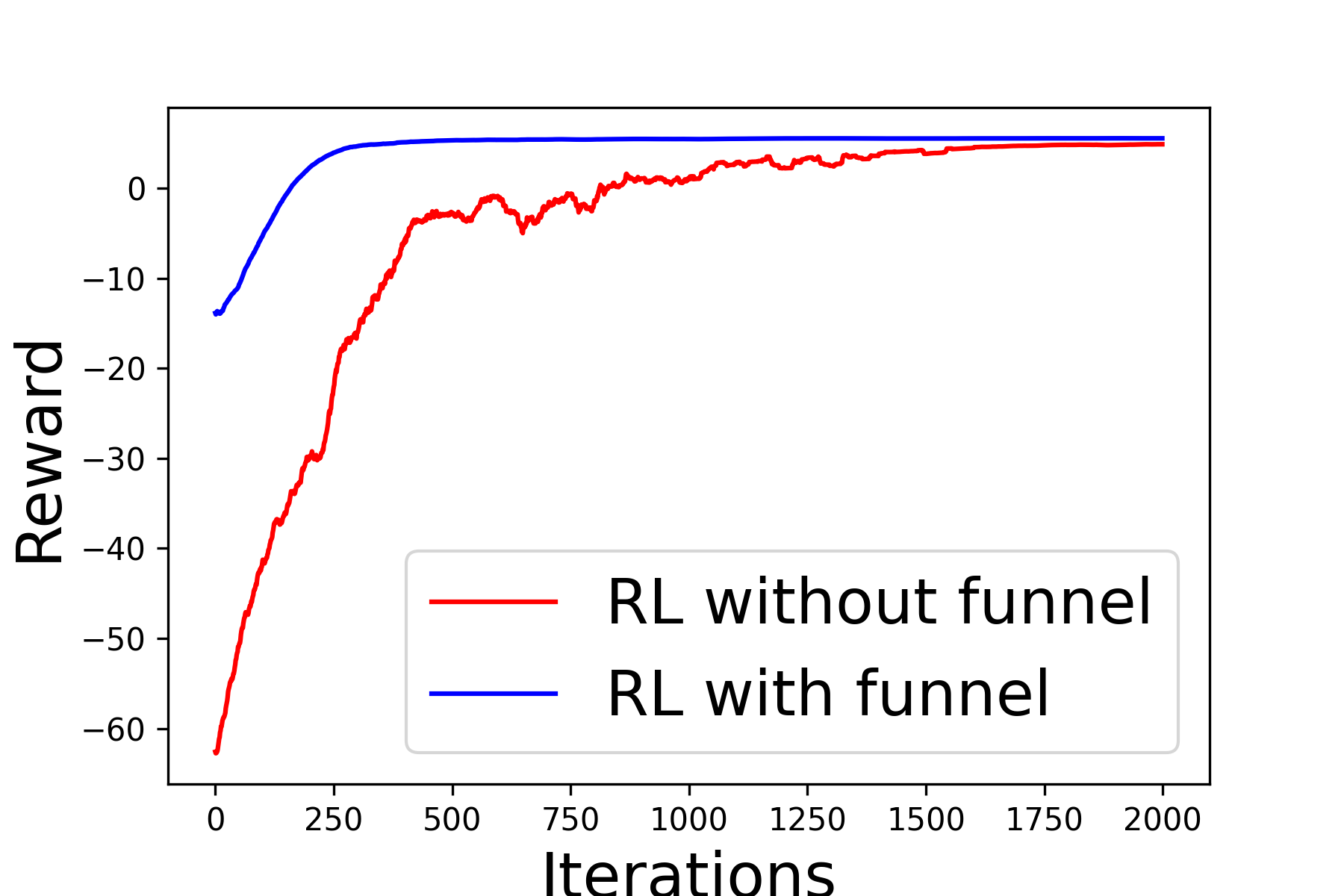
Figure 4: Reward during the training for the approach with and without the funnel controller.

In order to show the effect of the funnel controller, we visualized the number of funnel violations in Figure 5. It is clear that the use of the funnel controller avoids a violation such that the value for the funnel RL approach is zero for every iteration step. Without a funnel, the number of violations in $100$ trajectories is high. Especially at the beginning of the training, every trajectory ends with a violation. Keep in mind that a violation could mean a collision of the satellite with its environment. After approximately $1000$ iterations the number of violations decreases and becomes zero at the end of the training since the RL algorithm learns to avoid it. Nevertheless, we do not have a guarantee that the final policy is safe.

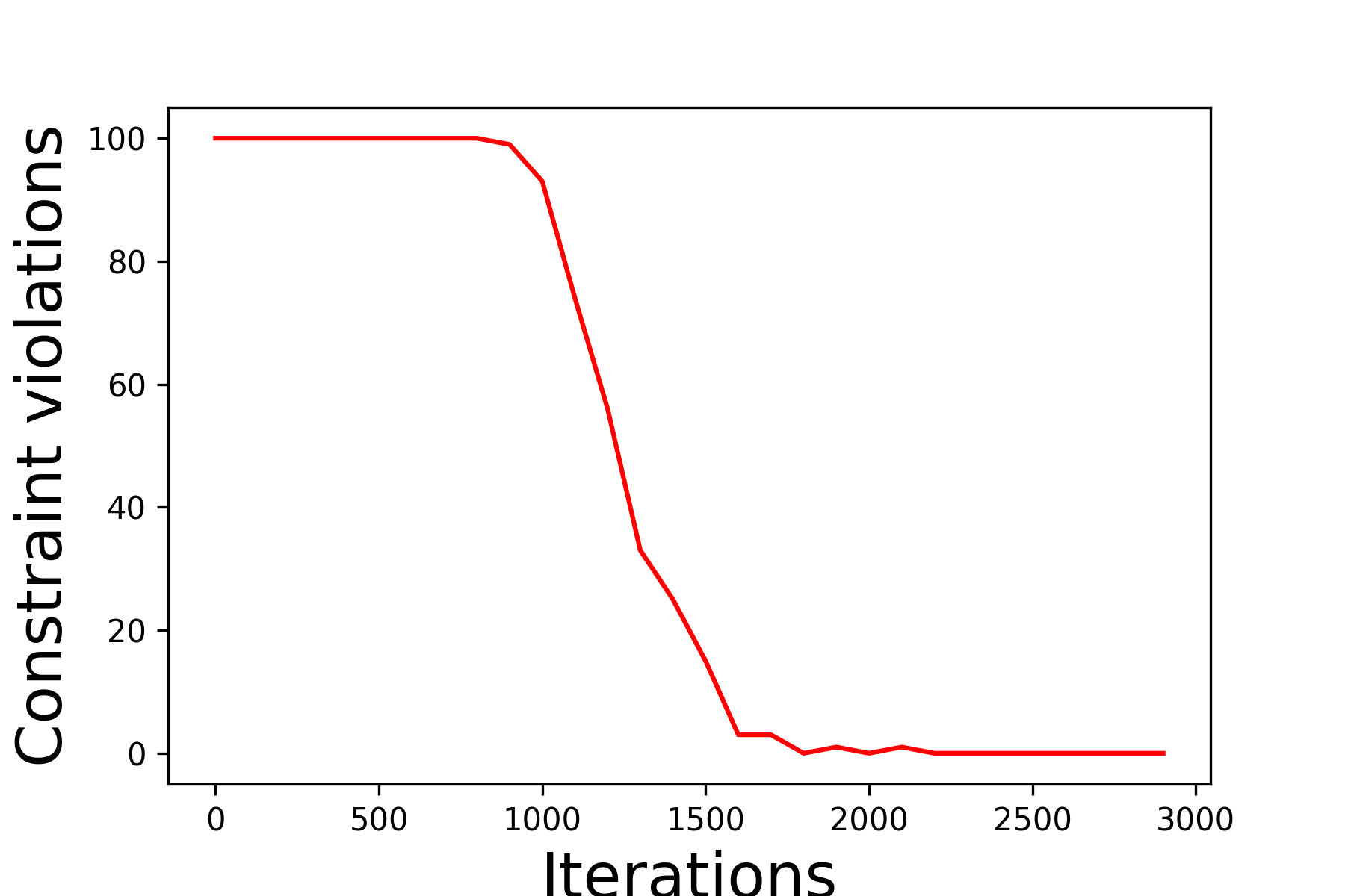
Figure 5: Number of constraint violations during the training of the approach without the funnel controller.

In the funnel-RL case, we are sure by construction that there are no funnel violations. Here, we have a look, how often the funnel controller has to intervene during the training to keep the training safe. In Figure 6, we observe that in the beginning, when the policy is not well trained, the funnel control is activated very often. However, little by little, the policy learns how to act such that the funnel controller does not have to intervene. At the end, there was no funnel control intervention needed to generate $100$ trajectories within the desired funnel.

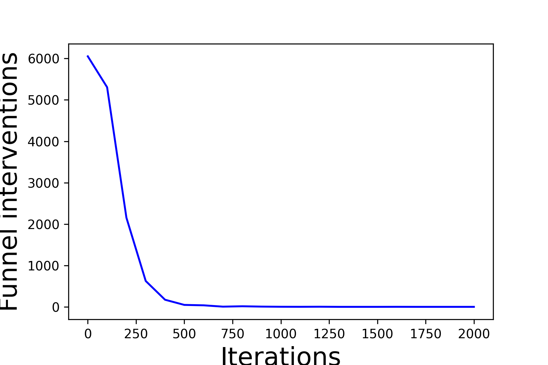
Figure 6: Number of funnel interventions during the training of the approach with the funnel controller.

In order to emphasize the effect of the funnel controller, in Figure 7, we plotted the $100$ trajectories of $\psi_{1}$ for the funnel-RL policy before the training. Thereby, the red thick lines represent the funnel. It can be seen that the trajectories are kept inside the funnel. But, in the area close to the reference trajectory the trajectories are chaotic, since the RL part is not trained yet.

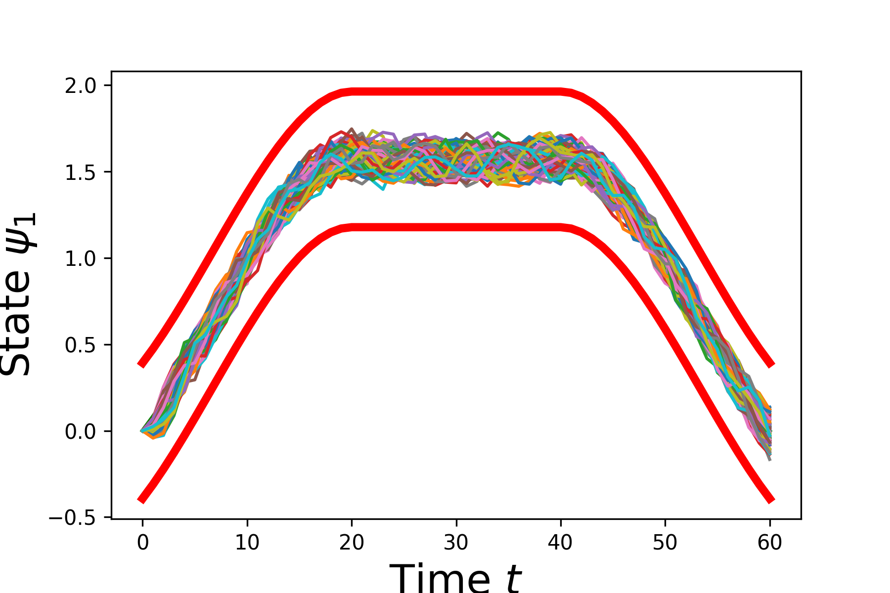
Figure 7: Generated trajectories for $\psi_{1}$ from an untrained policy with funnel controller.

For comparison, we plotted $100$ trajectories for the same state $\psi_{1}$ after the training in Figure 8. The trajectories are still inside the funnel, but now, all trajectories show a similar behavior due to the trained RL policy.

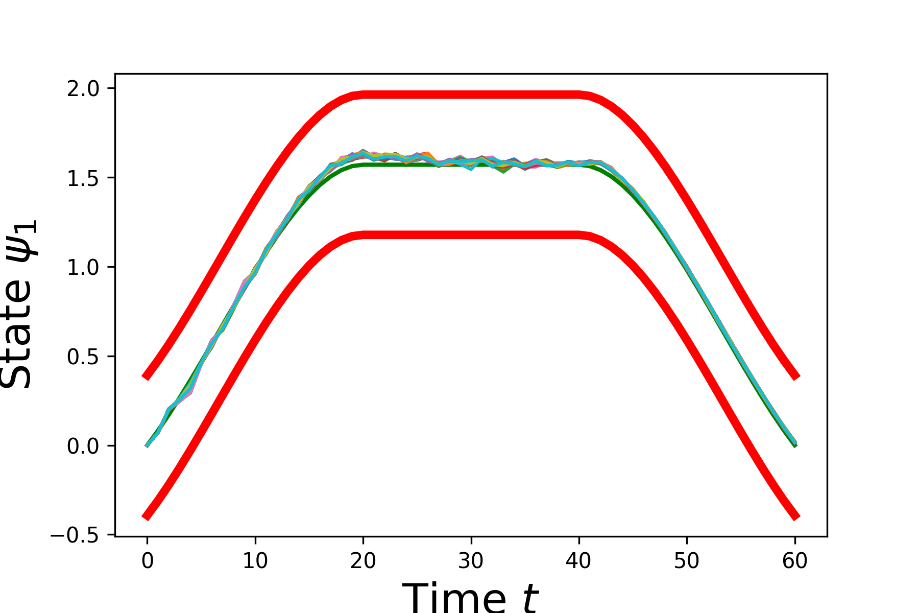
Figure 8: Generated trajectories from the trained policy with funnel controller.

Overall, we have received a fast controller, which is able to perform the docking maneuver and is protected against collisions with obstacles outside the safety funnel.

5 Conclusion

To safely conduct docking maneuvers in orbit, we introduced a two-component controller. One component is an optimal control policy derived from system data using Reinforcement Learning. To safeguard the learning process and compensate undesired control actions, we add a high-gain adaptive controller into the control algorithm, which is activated based on evaluations whether the system is in a safe or a safety-critical region. Effectiveness of the proposed controller is demonstrated by a numerical example of a satellite docking maneuver with collision avoidance. In future research we will focus on the design of an overall control algorithm where the assignment of safe and safety-critical regions accounts for uncertainties both in the model parameters and the trustworthiness of the training state

References

- Berger et al. (2023) Berger, T., Dennstädt, D., Lanza, L., and Worthmann, K. (2023). Robust funnel model predictive control for output tracking with prescribed performance. Preprint arXiv:2302.01754.
- Berger et al. (2021a) Berger, T., Drücker, S., Lanza, L., Reis, T., and Seifried, R. (2021a). Tracking control for underactuated non-minimum phase multibody systems. Nonlinear Dynamics, 104(4), 3671–3699.
- Berger et al. (2021b) Berger, T., Ilchmann, A., and Ryan, E.P. (2021b). Funnel control of nonlinear systems. Mathematics of Control, Signals, and Systems, 33, 151–194.
- Berthier (2022) Berthier, E. (2022). Efficient Algorithms for Control and Reinforcement. Ph.D. thesis, Université PSL (Paris Sciences & Lettres).
- Berthier et al. (2021) Berthier, E., Carpentier, J., and Bach, F. (2021). Fast and robust stability region estimation for nonlinear dynamical systems. In 2021 European Control Conference (ECC), 1412–1419.
- Bertsekas (2019) Bertsekas, D. (2019). Reinforcement Learning and Optimal Control. Athena Scientific optimization and computation series. Athena Scientific.
- Drücker et al. (2023) Drücker, S., Lanza, L., Berger, T., Reis, T., and Seifried, R. (2023). Experimental validation for the combination of funnel control with a feedforward control strategy. Preprint arXiv:2312.04380.
- Elhaki et al. (2023) Elhaki, O., Shojaei, K., Moghtaderizadeh, I., and Sajadian, S.J. (2023). Reinforcement learning-based saturated adaptive robust output-feedback funnel control of surface vessels in different weather conditions. Journal of the Franklin Institute, 360(18), 14237–14260.
- Ilchmann et al. (2002) Ilchmann, A., Ryan, E.P., and Sangwin, C.J. (2002). Tracking with prescribed transient behaviour. ESAIM: Control, Optimisation and Calculus of Variations, 7, 471–493.
- Kortüm and Lugner (1993) Kortüm, W. and Lugner, P. (1993). Systemdynamik und Regelung von Fahrzeugen: Einführung und Beispiele. Springer Berlin Heidelberg.
- Lanza et al. (2023a) Lanza, L., Dennstädt, D., Berger, T., and Worthmann, K. (2023a). Safe continual learning in MPC with prescribed bounds on the tracking error. Preprint arXiv:2304.10910.
- Lanza et al. (2023b) Lanza, L., Dennstädt, D., Worthmann, K., Schmitz, P., Sen, G., Trenn, S., and Schaller, M. (2023b). Control and safe continual learning of output-constrained nonlinear systems. Preprint arXiv:2303.00523.
- Liang et al. (2018) Liang, E., Liaw, R., Nishihara, R., Moritz, P., Fox, R., Goldberg, K., Gonzalez, J., Jordan, M., and Stoica, I. (2018). RLlib: Abstractions for distributed reinforcement learning. In J. Dy and A. Krause (eds.), Proceedings of the 35th International Conference on Machine Learning, volume 80 of Proceedings of Machine Learning Research, 3053–3062. PMLR.
- Saxena et al. (2023) Saxena, N., Sandeep, G., and Jagtap, P. (2023). Funnel-based reward shaping for signal temporal logic tasks in reinforcement learning. Preprint arXiv:2212.03181v3.
- Schmitz et al. (2023) Schmitz, P., Lanza, L., and Worthmann, K. (2023). Safe data-driven reference tracking with prescribed performance. In 2023 27th International Conference on System Theory, Control and Computing (ICSTCC), 454–460. IEEE.
- Schulman et al. (2015) Schulman, J., Levine, S., Abbeel, P., Jordan, M.I., and Moritz, P. (2015). Trust region policy optimization. In F.R. Bach and D.M. Blei (eds.), ICML, volume 37 of JMLR Workshop and Conference Proceedings, 1889–1897. JMLR.org.
- Schulman et al. (2017) Schulman, J., Wolski, F., Dhariwal, P., Radford, A., and Klimov, O. (2017). Proximal policy optimization algorithms. Preprint arXiv:1707.06347.
- Xia et al. (2023) Xia, K., Huang, Y., Zou, Y., and Zuo, Z. (2023). Reinforcement learning control for moving target landing of vtol uavs with motion constraints. IEEE Transactions on Industrial Electronics, 1–10.